Stable Prediction with Model Misspecification and Agnostic Distribution Shift

Abstract

For many machine learning algorithms, two main assumptions are required to guarantee performance. One is that the test data are drawn from the same distribution as the training data, and the other is that the model is correctly specified. In real applications, however, we often have little prior knowledge on the test data and on the underlying true model. Under model misspecification, agnostic distribution shift between training and test data leads to inaccuracy of parameter estimation and instability of prediction across unknown test data. To address these problems, we propose a novel Decorrelated Weighting Regression (DWR) algorithm which jointly optimizes a variable decorrelation regularizer and a weighted regression model. The variable decorrelation regularizer estimates a weight for each sample such that variables are decorrelated on the weighted training data. Then, these weights are used in the weighted regression to improve the accuracy of estimation on the effect of each variable, thus help to improve the stability of prediction across unknown test data. Extensive experiments clearly demonstrate that our DWR algorithm can significantly improve the accuracy of parameter estimation and stability of prediction with model misspecification and agnostic distribution shift.

Introduction

Predicting unknown outcomes based on a model estimated on a training data set is a common machine learning problem. Many machine learning algorithms have been proposed and shown to be very successful for prediction when the test data have the same distribution as the training data or the model specification is correct. In real applications, however, we rarely know the underlying true model for prediction, and we cannot guarantee the unknown test data will have the same distribution as the training data. For example, different geographies, schools, or hospitals may draw from different demographics, and the correlation structure among demographics may also vary (e.g. one ethnic group may be more or less disadvantaged in different geographies). If the model is misspecified, it may exploit subtle statistical relationships among features present in the training data to improve prediction, resulting in inaccuracy of parameter estimation and instability of prediction across test data sets with different distributions.

To correct the distribution shift between training and test data, many methods have been proposed in domain adaption (?; ?) and transfer learning (?). The motivation of these methods is to adjust the distribution of training data to mimic the distribution of test data, so that a predictive algorithm trained on training data can minimize the predictive error on test data. These methods achieve good performance in practice, however, they require the test data as prior knowledge. Hence, they cannot be applied to address the agnostic distribution shift problem.

Recently, some algorithms have been proposed to address the agnostic distribution shift from unknown test data, including domain generalization (?), causal transfer learning (?) and invariant causal prediction (?) etc. Their motivation is to explore the invariant structure between predictors and the response variable across multiple training datasets for prediction. But they cannot well handle the case of distribution shifts that are not observed in the training data. Moreover, they do not consider the interaction of distribution shift and model misspecification. Recently, some papers (?; ?) were proposed to address stable prediction problem using methods drawn from the literature on causal inference, achieving improved performance. But they did not consider the model misspecification and their algorithms were restricted to the predictive setting with binary predictors and binary response variable.

In this paper, we focus on the problem of stable prediction with model misspecification and agnostic distribution shift, where we assume that all features (predictors) $\mathbf{X}$ fall into one of two categories: one category includes the stable features $\mathbf{S}$, which have causal effects on outcome $Y$ that are invariant across environments (e.g., across training and test sets). The other category includes the unstable features $\mathbf{V}$, which have no causal effects on outcome, but may be correlated with either stable features, the outcome, or both. The correlation may be different in different environments. Under the assumption that all stable features are observed, model misspecification would be induced by some omitted nonlinear or interaction terms of stable features (i.e., $s_{1}\cdot s_{2}$ or $e^{s_{1}\cdot s_{2}}$). Since different environments (e.g., training and test sets) have different covariate distributions, the parameters estimated from different environments may be quite different even when we use the same parametric model. This variation in parameters arises because the parameters on included features capture two components: first, the partial effect of the included features on the expected value of outcome, and second, a function that depends on the correlation between included and omitted features, as well the distribution of outcomes conditional on omitted features. We consider the the problem of making predictions when that second component of estimated parameters is unstable across environments. In that case, we prefer to find an estimator that eliminates the second component, even though including it improves prediction for test sets that are similar to the training data. We look for an algorithm that is effective when the analyst does not know which feature is stable feature and which is not.

One way to address the problem of stable prediction in such a setting is to isolate the impact of each individual feature. One method commonly used in the causal literature is covariate balancing (?; ?; ?), which essentially estimates the impact of the target feature by reweighting the data so that the distribution of covariates is equalized across different values of the target feature. This literature usually focuses on the case where there is a single, pre-specified feature of interest and other features are considered to be “confounders”. In this paper, we consider the case where there are potentially many stable features, and propose a novel Decorrelated Weighting Regression (DWR) algorithm for stable prediction with model misspecification and agnostic distribution shift by jointly optimizing a variable decorrelation regularizer and a weighted regression model. Specifically, the variable decorrelation regularizer constructs sample weights to reduce correlation among covariates and allows the weighted regression to approximately isolate the effect of each variable. The weighted regression model with those sample weights might perform worse than standard methods when predicting in the test data with similar distribution to the training, but it will do better across unknown test data with distribution shift from the training. Using both empirical experiments and theoretical analysis, we show that our algorithm outperforms alternatives in parameter estimation and stability in prediction across unknown test data.

This paper has three main contributions: 1) we investigate the problem of stable prediction with model misspecification and agnostic distribution shift. The problem setting is more general and practical than prior work. 2) We propose a novel DWR algorithm to jointly optimize variable decorrelation and weighted regression to address the stable prediction problem. 3) We conduct extensive experiments in both synthetic and real-world datasets to demonstrate the advantages of our algorithm on stable prediction problem.

Problem and Our Algorithm

In this section, we first give the formulation of stable prediction problem, then introduce the details of our algorithm.

Stable Prediction Problem

Let $\mathcal{X}$ denote the space of observed features and $\mathcal{Y}$ denote the outcome space. We define an environment to be a joint distribution $P_{XY}$ on $\mathcal{X}\times\mathcal{Y}$, and let $\mathcal{E}$ denote the set of all environments. In each environment $e\in\mathcal{E}$, we have dataset $D^{e}=(\mathbf{X}^{e},Y^{e})$, where $\mathbf{X}^{e}\in\mathcal{X}$ are predictor variables and $Y^{e}\in\mathcal{Y}$ is a response variable. The joint distribution of features and outcomes on $(\mathbf{X},Y)$ can change across environments: $P^{e}_{XY}\neq P^{e^{\prime}}_{XY}$ for $e,e^{\prime}\in\mathcal{E}$.

In this paper, our goal is to learn a predictive model for stable prediction with model misspecification and agnostic distribution shift. To measure its performance on stable prediction problem, we adopt the $Average\_Error$ and $Stability\_Error$ in (?) as:

where $|\mathcal{E}|$ refers to the number of test environments, and $RMSE(D^{e})$ represents the Root Mean Square Error of a predictive model on dataset $D^{e}$. Actually, $Average\_Error$ and $Stability\_Error$ refer to the mean and variance of predictive error over all possible environments $e\in\mathcal{E}$.

Then, the stable prediction problem (?) is defined as:

Problem 1 (Stable Prediction)

Given one training environment $e\in\mathcal{E}$ with dataset $D^{e}=(\mathbf{X}^{e},Y^{e})$, the task is to learn a predictive model to predict across unknown environment $\mathcal{E}$ with not only small $Average\_Error$ but also small $Stability\_Error$.

Letting $\mathbf{X}=\{\mathbf{S},\mathbf{V}\}$, we define $\mathbf{S}$ as stable features, and $\mathbf{V}$ as unstable features with Assumption 1:

Assumption 1

There exists a stable function f(s) such that for all environment $e\in\mathcal{E}$, $\mathbb{E}(Y^{e}|\mathbf{S}^{e}=s,\mathbf{V}^{e}=v)=\mathbb{E}(Y^{e}|\mathbf{S}^{e}=s)=f(s)$.

Assumption 1 can be guaranteed by $Y\perp\mathbf{V}|\mathbf{S}$. Thus, we can address the stable prediction problem by developing a predictive model that learns the stable function $f(\mathbf{S})$. But we have NO prior knowledge on which features are stable and which are unstable.

Assumption 2

All stable features $\mathbf{S}$ are observed.

Under Assumption 2, model misspecification will be induced when estimating an outcome function if the model omits some nonlinear transformations and interaction terms of the stable features. Suppose that the true stable function $f(\mathbf{S})$ and $Y$ in environment $e$ is given by:

$$Y^{e}=f(\mathbf{S}^{e})+\mathbf{V}^{e}\beta_{V}+\epsilon^{e}=\mathbf{S}^{e}\beta_{S}+g(\mathbf{S}^{e})+\mathbf{V}^{e}\beta_{V}+\varepsilon^{e}.$$ (3)

where $\beta_{V}=0$ and $\varepsilon^{e}\perp\mathbf{X}^{e}$. We assume that the analyst misspecifies the model by omitting $g(\mathbf{S}^{e})$ and uses a linear model for prediction.

Under Assumption 1, the distribution shift across environments is mainly induced by the variation in the joint distribution over $(\mathbf{V}^{e},\mathbf{S}^{e})$. Simple linear regression may estimate nonzero effects of unstable features $\mathbf{V}^{e}$ when $\mathbf{V}^{e}$ is correlated with the omitted variables $g(\mathbf{S}^{e})$. For OLS, we have

$$+ \scalebox{0.9}{$(\frac{1}{n}\sum\limits_{i=1}^{n}\mathbf{V}_{i}^{T}\mathbf{V}_{i})^{-1}(\frac{1}{n}\sum\limits_{i=1}^{n}\mathbf{V}_{i}^{T}\mathbf{S}_{i})(\beta_{S}-\hat{\beta}_{S_{OLS}})$},$$

$$+ \scalebox{0.9}{$(\frac{1}{n}\sum\limits_{i=1}^{n}\mathbf{S}_{i}^{T}\mathbf{S}_{i})^{-1}(\frac{1}{n}\sum\limits_{i=1}^{n}\mathbf{S}_{i}^{T}\mathbf{V}_{i})(\beta_{V}-\hat{\beta}_{V_{OLS}})$},$$

where $n$ is sample size, $\frac{1}{n}\sum_{i=1}^{n}\mathbf{V}_{i}^{T}g(\mathbf{S}_{i})=\mathbb{E}(\mathbf{V}^{T}g(\mathbf{S}))+o_{p}(1)$ and $\frac{1}{n}\sum_{i=1}^{n}\mathbf{V}_{i}^{T}\mathbf{S}_{i}=\mathbb{E}(\mathbf{V}^{T}\mathbf{S})+o_{p}(1)$. To simplify notation, we remove the environment variable $e$ from $\mathbf{X}^{e}$, $\mathbf{S}^{e}$, $\mathbf{V}^{e}$, $\varepsilon^{e}$.

If $\mathbb{E}(\mathbf{V}^{T}g(\mathbf{S}))\neq 0$ or $\mathbb{E}(\mathbf{V}^{T}\mathbf{S})\neq 0$ in Eq. (4), $\hat{\beta}_{V_{OLS}}$ will be biased, resulting in the biased estimation on $\mathbf{S}$ in Eq. (5). And its prediction will be very unstable since the correlation between $\mathbf{V}$ and $g(\mathbf{S})$ (or $\mathbf{S}$) might vary across testing environments. Hence, to increase the stability of prediction, we need to precisely estimate the parameters of $\hat{\beta}_{V_{OLS}}$ by removing the correlation between $\mathbf{V}$ and $g(\mathbf{S})$ (or $\mathbf{S}$) on training data, that is let $\mathbb{E}(\mathbf{V}^{T}g(\mathbf{S}))=0$ and $\mathbb{E}(\mathbf{V}^{T}\mathbf{S})=0$.

Notations. In our paper, $n$ refers to the sample size, and $p$ is the dimensions of variables. For any vector $\textbf{v}\in\mathbb{R}^{p\times 1}$, let $\|\textbf{v}\|_{2}^{2}=\sum_{i=1}^{p}v_{i}^{2}$, and $\|\textbf{v}\|_{1}=\sum_{i=1}^{p}|v_{i}|$. For any matrix $\mathbf{X}\in\mathbb{R}^{n\times p}$, we let $\mathbf{X}_{i,}$ and $\mathbf{X}_{,j}$ represent the $i^{th}$ sample and the $j^{th}$ variable in $\mathbf{X}$, respectively.

Variable Decorrelation

In this subsection, we introduce our variable decorrelation regularizer to reduce the correlation between $\mathbf{V}$ and $\mathbf{S}$ (or $g(\mathbf{S})$) in the training environment.

Proposition 1

If $\mathbf{X}$ are mutually independent with mean 0, then $\mathbb{E}(\mathbf{V}^{T}g(\mathbf{S}))=0$ and $\mathbb{E}(\mathbf{V}^{T}\mathbf{S})=0$.

Proposition 1 together with Eq. (4) and Eq. (5) imply that if the covariates are mutually independent, we can unbiasedly estimate parameter $\beta_{V}$ even $g(\mathbf{S})$ is omitted. This motivates our regularizer.

From (?), we know variables $\mathbf{X}_{,j}$ and $\mathbf{X}_{,k}$ are independent if $\mathbb{E}[\mathbf{X}_{,j}^{a}\mathbf{X}_{,k}^{b}]=\mathbb{E}[\mathbf{X}_{,j}^{a}]\mathbb{E}[\mathbf{X}_{,k}^{b}]$ for all $a,b\in\mathbb{N}$. Inspired by the weighting methods in the causal literature (?; ?; ?), we propose to make $\mathbf{X}_{,j}$ and $\mathbf{X}_{,k}$ become independent by reweighting samples with weights $W$, which can be learnt with the following objective function:

$$\scalebox{1.0}{$\min\limits_{W}\sum\limits_{a=1}^{\infty}\sum\limits_{b=1}^{\infty}\|\mathbb{E}[\mathbf{X}_{,j}^{a^{T}}\mathbf{\Sigma}_{W}\mathbf{X}_{,k}^{b}]-\mathbb{E}[\mathbf{X}_{,j}^{a^{T}}W]\mathbb{E}[\mathbf{X}_{,k}^{b^{T}}W]\|_{2}^{2}$},$$ (6)

where $W\in\mathbb{R}^{n\times 1}$ are sample weights, $\sum_{i=1}^{n}W_{i}=n$ and $\mathbf{\Sigma}_{W}=diag(W_{1},\cdots,W_{n})$ is the corresponding diagonal matrix. In practice, however, it will not be feasible to attain the objective that all the moments of variables in the objective function from Eq. (6) are equal to zero. Fortunately, from Eq. (4) and Eq. (5) we know that reducing correlation among the first moments of the variables can help to improve the precision of parameter estimation and the stability of predictive models, and in practice the analyst can include high-order moments, for example, polynomial functions of covariates to further improve stability.

In this paper, we focus on variables’ first moment and propose to de-correlate all the predictors by sampling reweighting in the training environment. Specifically, we propose a variable decorrelation regularizer for learning that sample weight $W$ as follows:

(7)

where $\mathbf{X}_{,-j}=\mathbf{X}\backslash\{\mathbf{X}_{,j}\}$ means all the remaining variables by removing the $j^{th}$ variable in $\mathbf{X}$. The summand represents the loss due to correlation between variable $\mathbf{X}_{,j}$ and all other variables $\mathbf{X}_{,-j}$. Note that, only first moment is considered in Eq. (7), but it is sufficient for variables decorrelation. And higher-order moments can be easily incorporated.

The following theoretical results (proved in the supplementary material) show that our variable decorrelation regularizer can make the variables in $\mathbf{X}$ become mutually uncorrelated by sample reweighting, hence reduce the correlation among covariates in the training environment and improve the accuracy on parameter estimation.

With $\sum_{i=1}^{n}W_{i}=n$, we can denote the loss in Eq. (7) as:

$$\scalebox{0.9}{$\mathcal{L}_{B}=\sum_{j=1}^{p}\left\lVert\mathbf{X}_{,j}^{T}\mathbf{\Sigma}_{W}\mathbf{X}_{,-j}/n-\mathbf{X}_{,j}^{T}W/n\cdot\mathbf{X}_{,-j}^{T}W/n\right\rVert_{2}^{2}$}.$$ (8)

Lemma 1

If the number of covariates $p$ is fixed, then there exists a sample weight $W\succeq 0$ such that

$$\lim\limits_{n\rightarrow\infty}\mathcal{L}_{B}=0$$ (9)

with probability $1$. In particular, a solution $W$ to Eq. (9) is $W_{i}^{\star}=\frac{\Pi_{j=1}^{p}\hat{f}(\mathbf{X}_{i,j})}{\hat{f}(\mathbf{X}_{i,1},\cdots,\mathbf{X}_{i,p})}$, where $\hat{f}(x_{\cdot,j})$ and $\hat{f}(x_{\cdot,1},\cdots,x_{\cdot,p})$ are the Kernel density estimators.

Proof 1

See Appendix.

But the solution $W$ that satisfies Eq. (9) in Lemma 1 is not unique. To address this problem, we propose to simultaneously minimize the variance of $W$ and restrict the sum of $W$ in our regularizer as follows:

$$\hat{W}=\arg\min\limits_{W\in\mathcal{C}}\mathcal{L}_{B}+\frac{\lambda_{3}}{n}\scalebox{1.0}{$\sum_{i=1}^{n}W_{i}^{2}$}+\lambda_{4}(\frac{1}{n}\scalebox{1.0}{$\sum_{i=1}^{n}W_{i}-1$})^{2},$$ (10)

where $\mathcal{C}=\{W:|W_{ij}|\leq c\}$ for some constant $c$.

Then, we have following theorem on our variable decorrelation regularizer in Eq. (10).

Theorem 1

The solution $\hat{W}$ defined in Eq. (10) is unique if $\lambda_{3}n\gg p^{2}+\lambda_{4}$, $p^{2}\gg\max(\lambda_{3},\lambda_{4})$ and $|\mathbf{X}_{i,j}|\leq c$ for some constant $c$.

Proof 2

See Appendix.

With Lemma 1 and Theorem 1, we can derive the following property of the $\hat{W}$ given by Eq. (10).

Property 1. When $p$ is fixed, $n\rightarrow\infty$, $\lambda_{3}n\gg p^{2}+\lambda_{4}$, and $p^{2}\gg\max(\lambda_{3},\lambda_{4})$, the variables in $\mathbf{X}$ become uncorrelated by sample reweighting with $\hat{W}$. Hence, correlation between $\mathbf{V}$ and $\mathbf{S}$ in the training environment will be removed.

Extensive empirical experiments demonstrate that the correlation between $\mathbf{V}$ and $g(\mathbf{S})$ will also be reduced by our regularizer. In summary, the proposed variable decorrelation regularizer in Eq. (10) can learn a unique optimal sample weights $\hat{W}$ that can de-correlate the variables $\mathbf{X}$, and thus improve the accuracy in parameters estimation and stability in prediction.

Decorrelated Weighting Regression

With the learned sample weights $\hat{W}$ from variable decorrelation regularizer in Eq. (10), one can run weighted least square (WLS) to estimate the regression coefficient $\beta$ as:

$$\hat{\beta}_{WLS}=\arg\min\limits_{\beta}\sum\limits_{i=1}^{n}\hat{W}_{i}\cdot(Y_{i}-\mathbf{X}_{i,}\beta)^{2}.$$ (11)

The $\hat{\beta}_{WLS}$ is expected to have less bias than $\hat{\beta}_{OLS}$ under Property 1, since sample reweighted by $\hat{W}$ de-correlates variables in $\mathbf{X}$.

By combining the objective functions of the variable decorrelation regularizer in Eq. (10) and the weighted regression in Eq. (11), we propose a Decorrelated Weighted Regression (DWR) algorithm to jointly optimize sample weights $W$ and regression coefficient $\beta$ as follows:

$$s.t \sum_{j=1}^{p}\left\lVert\mathbf{X}_{,j}^{T}\mathbf{\Sigma}_{W}\mathbf{X}_{,-j}/n-\mathbf{X}_{,j}^{T}W/n\cdot\mathbf{X}_{,-j}^{T}W/n\right\rVert_{2}^{2}<\lambda_{2}$$

$$\scalebox{1.0}{$|\beta|_{1}<\lambda_{1},\ \ \frac{1}{n}\sum_{i=1}^{n}W_{i}^{2}<\lambda_{3}$},$$

$$(\frac{1}{n}\sum_{i=1}^{n}W_{i}-1)^{2}<\lambda_{4},\ \ W\succeq 0,$$

where $n$ denotes the sample size, $p$ refers to the dimension of variables $\mathbf{X}$. $\mathbf{X}_{i,}$ and $\mathbf{X}_{,j}$ represent the $i^{th}$ sample and the $j^{th}$ variable in $\mathbf{X}$, respectively. The term $W\succeq 0$ constrains each sample weight to be non-negative. With term $\frac{1}{n}\sum_{i=1}^{n}W_{i}^{2}<\lambda_{3}$, we reduce the variation of the sample weights. The term $(\frac{1}{n}\sum_{i=1}^{n}W_{i}-1)^{2}<\lambda_{4}$ avoids all sample weights to be $zero$.

Algorithm 1 Decorrelated Weighted Regression algorithm

1:Observed features $\mathbf{X}$ and outcome variable $Y$.

2:Updated parameters $W$, $\beta$.

3:Initialize parameters $W^{(0)}$ and $\beta^{(0)}$,

4:Calculate loss function with parameters $(W^{(0)},\beta^{(0)})$,

5:Initialize the iteration variable $t\leftarrow 0$,

6:repeat

7:     $t\leftarrow t+1$,

8:     Update $W^{(t)}$ with gradient descent by fixing $\beta$,

9:     Update $\beta^{(t)}$ with gradient descent by fixing $W$,

10:     Calculate loss function with parameters $(W^{(t)},\beta^{(t)})$,

11:until Loss function converges or max iteration is reached.

12:return $W$, $\beta$.

Optimization and Analysis

Optimization

To optimize our DWR algorithm in Eq. (Decorrelated Weighting Regression), we propose an iterative method. Firstly, we initialize sample weights $W_{i}=1$ for each sample $i$ and regression coefficient $\beta=[0,0,\cdots,0]^{T}$. Once the initial values are given, in each iteration, we first update $W$ by fixing $\beta$, then update $\beta$ by fixing $W$ until the objective function in Eq. (Decorrelated Weighting Regression) converges. The whole algorithm is summarized in Algorithm 1.

Complexity Analysis

In our DWR algorithm, the main time cost is to calculate the value of loss function and update parameters $W$ and $\beta$ in each iteration. The complexity of calculating the loss function is $O(np^{2})$, where $n$ is the sample size and $p$ refers to the dimension of observed variables. The complexity of updating parameter $W$ is also $O(np^{2})$. The complexity of updating parameter $\beta$ is $O(np)$.

In total, the complexity of each iteration in Algorithm 1 is $O(np^{2})$.

Experiments

In this section, we check the performance of our algorithm with experiments on both synthetic and real-world datasets.

Baselines

We use following four methods as the baselines.

• Ordinary Least Square (OLS):

  $$\min\|Y-\mathbf{X}\beta\|_{2}^{2}.$$

• Lasso (?):

  $$\min\|Y-\mathbf{X}\beta\|_{2}^{2}+\lambda_{1}\|\beta\|_{1}.$$

• Ridge Regression (?):

  $$\min\|Y-\mathbf{X}\beta\|_{2}^{2}+\lambda_{1}\|\beta\|_{2}.$$

• Independently Interpretable Lasso (IILasso) (?)

  $$\min\|Y-\mathbf{X}\beta\|_{2}^{2}+\lambda_{1}\|\beta\|_{1}+\lambda_{2}|\beta|^{T}\mathbf{R}|\beta|,$$

  where $\mathbf{R}\in\mathcal{R}^{p\times p}$ with each element $\mathbf{R}_{jk}=|r_{jk}|/(1-|r_{jk}|)$, and $r_{jk}=\frac{1}{n}|\mathbf{X}_{,j}^{T}\mathbf{X}_{,k}|$.

To avoid the degeneration of above baselines, we set their hype-parameters $\lambda_{1}\neq 0$ and $\lambda_{2}\neq 0$.

Evaluation Metrics

To evaluate the performance of stable prediction, we use $RMSE$, $\beta\_Error$, $Average\_Error$ and $Stability\_Error$ as evaluation metrics. Their definitions of $RMSE$ and $\beta\_Error$ are listed as follows:

$$\scalebox{1.0}{$RMSE=\sqrt{\frac{1}{n}\sum_{k=1}^{n}(Y_{k}-\hat{Y}_{k})}$},$$ (13)

where $n$ is sample size, $\hat{Y}_{k}$ and $Y_{k}$ refer to the predicted and true outcome for sample $k$.

$$\scalebox{1.0}{$\beta\_Error=\|\beta-\hat{\beta}\|_{1}$},$$ (14)

where $\hat{\beta}$ and $\beta$ represent the estimated and true regression coefficients.

Experiments on Synthetic Data

Dataset

Under Assumption 1, there are three kinds of relationships between $\mathbf{X}=\{\mathbf{S},\mathbf{V}\}$ and $Y$ as shown in Fig. 1, including $\mathbf{S}\perp\mathbf{V}$, $\mathbf{S}\rightarrow\mathbf{V}$, and $\mathbf{V}\rightarrow\mathbf{S}$. We consider settings motivated by each of the three cases as follows:

$\mathbf{S}\perp\mathbf{V}$: In this setting, $\mathbf{S}$ and $\mathbf{V}$ are independent, but $\mathbf{S}$ could be dependent with each other. Hence, we generate $\mathbf{X}=\{\mathbf{S}_{,1},\cdots,\mathbf{S}_{,p_{s}},\mathbf{V}_{,1},\cdots,\mathbf{V}_{,p_{v}}\}$ with independent Gaussian distributions with the help of auxiliary variables $\mathbf{Z}$ as following:

$$\scalebox{1.0}{$\mathbf{Z}_{,1},\cdots,\mathbf{Z}_{,p}\ \overset{iid}{\sim}\mathcal{N}(0,1)$},\scalebox{1.0}{$\mathbf{V}_{,1},\cdots,\mathbf{V}_{,p_{v}}\ \overset{iid}{\sim}\mathcal{N}(0,1)$}$$ (15)

$$\mathbf{S}_{,i}=0.8*\mathbf{Z}_{,i}+0.2*\mathbf{Z}_{,i+1},\,\,i=1,2,\cdots,p_{s},$$ (16)

where the number of stable variables $p_{s}=0.5*p$ and the number of unstable variables $p_{v}=0.5*p$. $\mathbf{S}_{,j}$ represents the $j^{th}$ variable in $\mathbf{S}$.

(a) $\mathbf{S}\perp\mathbf{V}$

(b) $\mathbf{S}\rightarrow\mathbf{V}$

(c) $\mathbf{V}\rightarrow\mathbf{S}$

Figure 1: Three diagrams for stable features $\mathbf{S}$, unstable features $\mathbf{V}$, and response variable $Y$.

$\mathbf{S}\rightarrow\mathbf{V}$: In this setting, the stable features $\mathbf{S}$ are the causes of unstable features $\mathbf{V}$. We first generate dependent stable features $\mathbf{S}$ with Eq. (16). Then, we generate unstable features $\mathbf{V}$ based on $\mathbf{S}$: $\mathbf{V}_{\cdot,j}=0.8*\mathbf{S}_{\cdot,j}+0.2*\mathbf{S}_{\cdot,j+1}+\mathcal{N}(0,1)$ , where we let $j+1=mod(j+1,p_{s})$. The function $mod(a,b)$ returns the modulus after division of $a$ by $b$.

$\mathbf{V}\rightarrow\mathbf{S}$: In this setting, unstable features $\mathbf{V}$ are the causes of stable features $\mathbf{S}$. We first generate the unstable features $\mathbf{V}$ with Eq. (15). Then, we generate the stable features $\mathbf{S}$ based on $\mathbf{V}$: $\mathbf{S}_{\cdot,j}=0.2*\mathbf{V}_{\cdot,j}+0.8*\mathbf{V}_{\cdot,j+1}+\mathcal{N}(0,1)$ , where we let $j+1=mod(j+1,p_{v})$.

To test the performance with different forms of missing nonlinear and interaction terms, we generate the outcome $Y$ from a polynomial nonlinear function ($Y_{poly}$) and an exponential one ($Y_{exp}$):

$$\!\!\!\!\!\!Y_{poly}\!\!\!\!\!\! = \!\!\!\!\!\!f(\mathbf{S})+\varepsilon=[\mathbf{S},\mathbf{V}]\cdot[\beta_{s},\beta_{v}]^{T}+\mathbf{S}_{\cdot,1}\mathbf{S}_{\cdot,2}\mathbf{S}_{\cdot,3}+\varepsilon,$$ (17)

$$\!\!\!\!\!\!Y_{exp}\!\!\!\!\!\! = \!\!\!\!\!\!f(\mathbf{S})+\varepsilon=[\mathbf{S},\mathbf{V}]\cdot[\beta_{s},\beta_{v}]^{T}+e^{\mathbf{S}_{\cdot,1}\mathbf{S}_{\cdot,2}\mathbf{S}_{\cdot,3}}+\varepsilon.$$ (18)

where $\beta_{s}=\{\frac{1}{3},-\frac{2}{3},1,-\frac{1}{3},\frac{2}{3},-1,\cdots\}$, $\beta_{v}=\vec{0}$, and $\varepsilon=\mathcal{N}(0,0.3)$.

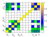
(a) On raw data

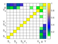
(b) On the weighted data

Figure 2: Pearson correlation coefficients among variables: a) on raw data; b) on weighted data.

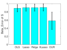
(a) $\beta$_Error of $\mathbf{S}$: Mean (green bar) and Variance (black line)

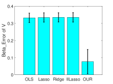
(b) $\beta$_Error of $\mathbf{V}$: Mean (green bar) and Variance (black line)

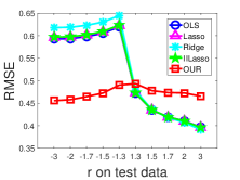
(c) RMSE over all test environments

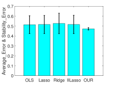
(d) Average_Error (green bar) $\&$ Stability Error (black line)

Figure 3: Results on $\mathbf{S}\perp\mathbf{V}$ with $Y=Y_{poly}$. All the models are trained with $n=2000$, $p=10$ and $r_{train}=1.7$.

Generating Various Environments

To test the stability of all algorithms, we need to generate a set of environments, each with a distinct joint distribution $P(\mathbf{X},Y)$, while preserving Assumption 1 (and in particular, $P(Y|\mathbf{S})$). Specifically, we generate different environments in our experiments by varying $P(\mathbf{V}|\mathbf{S})$. For simplification we only change $P(\mathbf{V}_{b}|\mathbf{S})$ on a subset of unstable features $\mathbf{V}_{b}\subseteq\mathbf{V}$, where the dimension of $\mathbf{V}_{b}$ is $0.1*p$.

Specifically, we vary $P(\mathbf{V}_{b}|\mathbf{S})$ via biased sample selection with a bias rate $r\in[-3,-1)\cup(1,3]$. For each sample, we select it with probability $Pr=\prod_{\mathbf{V}_{i}\in\mathbf{V}_{b}}|r|^{-5*D_{i}}$, where $D_{i}=|f(\mathbf{S})-sign(r)*\mathbf{V}_{i}|$. If $r>0$, $sign(r)=1$; otherwise, $sign(r)=-1$. $f(\mathbf{S})$ is defined in Eq. (17) or (18).

Note that $r>1$ corresponds to positive unstable correlation between $Y$ and $\mathbf{V}_{b}$, while $r<-1$ refers to the negative unstable correlation between $Y$ and $\mathbf{V}_{b}$. The higher the value of $|r|$, the stronger correlation between $\mathbf{V}_{b}$ and $Y$. Different value of $r$ refers to different environments, hence we can generate different environments by varying $P(\mathbf{V}_{b}|\mathbf{S})$.

Experimental Settings

In experiments, we evaluate the performance of all algorithms from two aspects, including accuracy on parameter estimation and stability on prediction across unknown test data. To measure the accuracy of parameter estimation, we train all models on one training dataset with a specific bias rate $r_{train}$. We carry out model training for 50 times independently with different training data from the same bias rate $r_{train}$, and report the mean and variance of $\beta\_Error$ on stable features $\mathbf{S}$ and unstable features $\mathbf{V}$. To evaluate the stability of prediction, we test all models on various test environments with different bias rate $r_{test}\in[-3,-1)\cup(1,3]$. For each test bias rate $r_{test}$, we generate 50 different test datasets and report the mean of RMSE. With RMSE from all test environments, we report Average$\_$Error and Stability$\_$Error to evaluate the stability of prediction across unknown test environments.

Table 1: Experimental results under setting $\mathbf{S}\perp\mathbf{V}$ with $Y=Y_{poly}$ when varying sample size $n$, dimension of variables $p$ and training bias rate $r$. The smaller value of $\beta_{S}$_Error, $\beta_{V}$_Error, Average_Error and Stability_Error, the better.

Scenario 1: varying sample size $n$
$n,p,r$	$n=1000,p=10,r=1.7$					$n=2000,p=10,r=1.7$					$n=4000,p=10,r=1.7$
	OLS	Lasso	Ridge	IILasso	Our	OLS	Lasso	Ridge	IILasso	Our	OLS	Lasso	Ridge	IILasso	Our
$\beta_{S}$_Error	0.892	0.907	0.907	0.912	0.578	0.887	0.903	0.903	0.908	0.581	0.906	0.921	0.921	0.926	0.614
$\beta_{V}$_Error	0.331	0.333	0.334	0.334	0.109	0.332	0.334	0.335	0.335	0.077	0.338	0.340	0.341	0.341	0.078
Average_Error	0.509	0.511	0.511	0.511	0.476	0.514	0.516	0.527	0.516	0.473	0.526	0.528	0.531	0.528	0.480
Stability_Error	0.084	0.086	0.086	0.086	0.012	0.090	0.092	0.103	0.092	0.012	0.104	0.105	0.108	0.106	0.015
Scenario 2: varying variables’ dimension $p$
$n,p,r$	$n=2000,p=10,r=1.5$					$n=2000,p=20,r=1.5$					$n=2000,p=40,r=1.5$
	OLS	Lasso	Ridge	IILasso	Our	OLS	Lasso	Ridge	IILasso	Our	OLS	Lasso	Ridge	IILasso	Our
$\beta_{S}$_Error	0.618	0.628	0.630	0.632	0.409	2.608	2.677	2.670	2.713	1.761	8.491	8.846	8.669	8.998	7.800
$\beta_{V}$_Error	0.243	0.245	0.246	0.245	0.052	0.426	0.433	0.433	0.437	0.260	0.661	0.684	0.673	0.694	0.606
Average_Error	0.486	0.487	0.487	0.487	0.476	0.523	0.527	0.539	0.529	0.480	0.532	0.540	0.537	0.543	0.490
Stability_Error	0.058	0.059	0.060	0.059	0.010	0.116	0.121	0.134	0.123	0.014	0.138	0.148	0.145	0.153	0.073
Scenario 3: varying bias rate $r$ on training data
$n,p,r$	$n=2000,p=10,r=1.5$					$n=2000,p=10,r=1.7$					$n=2000,p=10,r=2.0$
	OLS	Lasso	Ridge	IILasso	Our	OLS	Lasso	Ridge	IILasso	Our	OLS	Lasso	Ridge	IILasso	Our
$\beta_{S}$_Error	0.618	0.628	0.630	0.632	0.409	0.887	0.903	0.903	0.908	0.581	1.232	1.249	1.245	1.257	0.651
$\beta_{V}$_Error	0.243	0.245	0.246	0.245	0.052	0.332	0.334	0.335	0.335	0.077	0.441	0.444	0.443	0.445	0.119
Average_Error	0.486	0.487	0.487	0.487	0.476	0.514	0.516	0.527	0.516	0.473	0.568	0.571	0.571	0.571	0.476
Stability_Error	0.058	0.059	0.060	0.059	0.010	0.090	0.092	0.103	0.092	0.012	0.144	0.147	0.147	0.147	0.008

Results

Before reporting the experimental results, we demonstrate the Pearson correlation coefficients between any two variables on both raw data and the weighed data by our algorithm in Figure 2. From the figures, we can find that in the raw data, the unstable features $\mathbf{V}_{5}$ is correlated with some stable features $\mathbf{S}$, and highly correlated with both omitted nonlinear term $g$ and outcome $Y$. Hence, the estimated coefficient of $\mathbf{V}_{5}$ in the baselines would be large, which should be $zero$ in a correctly specified model, leading to unstable prediction. In the weighted data, the sample weights learnt from our algorithm can clearly remove the correlation among predictors $\mathbf{X}$. Moreover, the unstable correlation between $\mathbf{V}_{5}$ and $g$ are significantly reduced, which is helpful to reduce the unstable correlation between $\mathbf{V}_{5}$ and $Y$, and then the correlations between stable features $\mathbf{S}$ and $Y$ conditional on $\mathbf{V}$ are enhanced. Hence, our algorithm can estimate the coefficient of both $\mathbf{S}$ and $\mathbf{V}$ more precisely. This is the key reason that our algorithm can make more stable predictions across unknown test environments.

We report the results of parameter estimation and stable prediction under setting $\mathbf{S}\perp\mathbf{V}$ with $Y=Y_{poly}$ in Figure 3 and Table 1. To save space, the experimental results of settings $\mathbf{S}\rightarrow\mathbf{V}$ and $\mathbf{V}\rightarrow\mathbf{S}$ with $Y=Y_{poly}$, and results with $Y=Y_{exp}$ are reported in online Appendix. From the results, we have following observations and analysis:

• OLS cannot address the stable prediction problem. The reason is that OLS is biased on both $\beta_{S}$ and $\beta_{V}$ estimation as we discussed in the theoretical section. Moreover, OLS will often predict large effects of the unstable features, which leads to instability across environments.

• Lasso, Ridge and IILasso perform even worse than OLS, since their regularizers will generally estimate larger coefficients on the unstable features $\mathbf{V}_{b}$. For example, Lasso selects a only a subset of predictors and exacerbates the omitted variables problem that already exists in our basic setup.

• Comparing with baselines, our algorithm achieves more stable prediction across different settings. By reducing the correlation among all predictors, our algorithm avoids using unstable features to proxy for omitted nonlinear functions of the stable features, ensuring less bias in the estimation of the effect of both stable features and unstable features. Hence, improve the stability of prediction.

• The performance of our algorithm is worse than baseline when $r_{test}>1.3$ on test data in Fig. 3c, but much better than baselines when $r_{test}<-1.3$. This is because the correlations between $\mathbf{V}_{b}$ and $Y$ are similar between training data ($r_{train}=1.7$) and test data when $r_{test}>1.3$, and that correlation can be exploited in prediction; in this setting, $\mathbf{V}$ is useful to proxy for omitted functions of $\mathbf{S}$. However, when $r_{test}<-1.3$, using $\mathbf{V}$ for prediction creates too much instability.

• By varying the sample size $n$, dimension of variables $p$, training bias rate $r_{train}$ and the form of missing nonlinear and interaction terms, our algorithm is consistently outperform than baselines on parameter estimation and stable prediction across unknown test data.

Overall, our proposed DWR algorithm can be applied to address the problem of stable prediction with model misspecification and agnostic distribution shift.

Parameter Analysis

In our DWR algorithm, we have some hype-parameters, including $\lambda_{1}$ for constraining the sparsity of regression coefficient, $\lambda_{2}$ for constraining the error of decorrelation regularizer, $\lambda_{3}$ for constraining the variance of the sample weights, and $\lambda_{4}$ for constraining the sum of sample weights to $n$. In our experiments, we tuned these parameters with cross validation by grid searching, and each parameter is uniformly varied from $\{0.01,0.1,1,10,100\}$. In Figure 4, we displayed $Average\_Error$ and $Stability\_Error$ with respect to $\lambda_{2}$. From the figures, we can find that when $\lambda_{2}<10$, $Average\_Error$ and $Stability\_Error$ monotonically decrease as we increase the value of hype-parameter $\lambda_{2}$. But when $\lambda_{2}>10$, those errors will slightly increase as we keep increasing the value of hype-parameter $\lambda_{2}$.

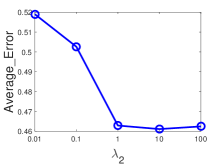
(a) $Average\_Error$ v.s. $\lambda_{2}$

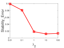
(b) $Stability\_Error$ v.s. $\lambda_{2}$

Figure 4: The effect of hype-parameter $\lambda_{2}$.

Experiments on Real World Data

Datasets and Experimental Setting

We collected air pollutant data and meteorological data from the U.S. EPA’s Air Quality System (AQS) database, which has been widely used for model evaluation (?; ?). The air pollutant data in this study is PM₁₀, and the meteorological variables are those would affect the air pollutant concentrations, including air temperature, relative humidity, pressure, wind speed and direction.

In our experiments, we let the outcome variable $Y$ be pollution PM₁₀, and set the meteorological features as the observed variables $\mathbf{X}$. To test the stability of all algorithms, we collected data from 10 different states in the U.S., where the states correspond to the different environments from the theory. Considering a practical setting where a researcher has a single data set and wishes to train a model that can then be applied to other related settings, in our experiments, we trained all models with data from State 1, validated with data from States 1 to 4, finally tested them on all 10 States.

To demonstrate the distribution difference between any two environments $e=i$ and $e=j$, we adopt the distribution distance between observed variables $\mathbf{X}$ as a metric with following definition:

where $p$ refers to the dimension of variables, and $\overline{\mathbf{X}}_{e=i}$ represents the mean value of variables $\mathbf{X}$ in environment $i$.

Results

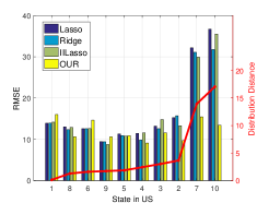
(a) RMSE v.s. Distribution Distance

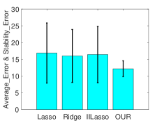
(b) Average$\_$Error (green bar) $\&$ Stability$\_$Error (black line)

Figure 5: Air quality prediction across different States in US. Models are trained on State 1. The red line represents the distance between training and test distribution.

We report the results of RMSE on air quality prediction over all 10 States in Fig. 5a, where we merged OLS method into Lasso by allowing its hype-parameter to be $zero$ during model training. The results show that the performance of our algorithm is worse than baselines when the distribution distance between training and test environments is small; in that case, we introduce variance by reweighting the data away from the distribution that approximates both training and test sets. But our algorithm’s performance improves relative to the baseline and ultimately becomes better than baseline as the distribution distance increases.

To explicitly demonstrate the advantage of our proposed algorithm, we report Average_Error and Stability_Error in Fig. 5b. The results show that our algorithm makes the most stable prediction with agnostic distribution shift on test data.

Conclusion

In this paper, we focus on how to facilitate a stable prediction across unknown test data, where we are concerned about two problems that together lead to instability: model misspecification, and agnostic distribution shift between training and test data. We proved that our algorithm can improve the accuracy of parameter estimation and stability on prediction from both theoretical analysis and empirical experiments. The experimental results on both synthetic and real-world datasets demonstrate that our algorithm outperforms the baselines for stable prediction across unknown test environments, when the correlation among covariates varies substantially across those environments.

Appendix: The online appendix and supplementary materials are available at http://kunkuang.github.io or https://www.dropbox.com/s/1q0brkc2bnehhfo/paper-aaai20-Supplementary.

References

- [Athey, Imbens, and Wager 2018] Athey, S.; Imbens, G. W.; and Wager, S. 2018. Approximate residual balancing: debiased inference of average treatment effects in high dimensions. Journal of the Royal Statistical Society: Series B (Statistical Methodology) 80(4):597–623.
- [Ben-David et al. 2010] Ben-David, S.; Blitzer, J.; Crammer, K.; Kulesza, A.; Pereira, F.; and Vaughan, J. W. 2010. A theory of learning from different domains. Machine learning 79(1-2):151–175.
- [Bickel, Brückner, and Scheffer 2009] Bickel, S.; Brückner, M.; and Scheffer, T. 2009. Discriminative learning under covariate shift. Journal of Machine Learning Research 10(Sep):2137–2155.
- [Bisgaard and Sasvári 2006] Bisgaard, T. M., and Sasvári, Z. 2006. When does e(xk·yl)=e(xk)·e(yl) imply independence? Statistics & Probability Letters 76(11):1111–1116.
- [Fong et al. 2018] Fong, C.; Hazlett, C.; Imai, K.; et al. 2018. Covariate balancing propensity score for a continuous treatment: application to the efficacy of political advertisements. The Annals of Applied Statistics 12(1):156–177.
- [Hoerl and Kennard 1970] Hoerl, A. E., and Kennard, R. W. 1970. Ridge regression: Biased estimation for nonorthogonal problems. Technometrics 12(1):55–67.
- [Kuang et al. 2017a] Kuang, K.; Cui, P.; Li, B.; Jiang, M.; Yang, S.; and Wang, F. 2017a. Treatment effect estimation with data-driven variable decomposition. In Thirty-First AAAI Conference on Artificial Intelligence, 140–146.
- [Kuang et al. 2017b] Kuang, K.; Cui, P.; Li, B.; Jiang, M.; and Yang, S. 2017b. Estimating treatment effect in the wild via differentiated confounder balancing. In Proceedings of the 23rd ACM SIGKDD International Conference on Knowledge Discovery and Data Mining, 265–274. ACM.
- [Kuang et al. 2018] Kuang, K.; Cui, P.; Athey, S.; Xiong, R.; and Li, B. 2018. Stable prediction across unknown environments. In Proceedings of the 24th ACM SIGKDD International Conference on Knowledge Discovery & Data Mining, 1617–1626. ACM.
- [Muandet, Balduzzi, and Schölkopf 2013] Muandet, K.; Balduzzi, D.; and Schölkopf, B. 2013. Domain generalization via invariant feature representation. In International Conference on Machine Learning, 10–18.
- [Pan and Yang 2009] Pan, S. J., and Yang, Q. 2009. A survey on transfer learning. IEEE Transactions on knowledge and data engineering 22(10):1345–1359.
- [Peters, Bühlmann, and Meinshausen 2016] Peters, J.; Bühlmann, P.; and Meinshausen, N. 2016. Causal inference by using invariant prediction: identification and confidence intervals. Journal of the Royal Statistical Society: Series B (Statistical Methodology) 78(5):947–1012.
- [Rojas-Carulla et al. 2018] Rojas-Carulla, M.; Schölkopf, B.; Turner, R.; and Peters, J. 2018. Invariant models for causal transfer learning. The Journal of Machine Learning Research 19(1):1309–1342.
- [Shen et al. 2018] Shen, Z.; Cui, P.; Kuang, K.; Li, B.; and Chen, P. 2018. Causally regularized learning with agnostic data selection bias. In ACM Multimedia, 411–419.
- [Takada, Suzuki, and Fujisawa 2017] Takada, M.; Suzuki, T.; and Fujisawa, H. 2017. Independently interpretable lasso: A new regularizer for sparse regression with uncorrelated variables. arXiv preprint arXiv:1711.01796.
- [Tibshirani 1996] Tibshirani, R. 1996. Regression shrinkage and selection via the lasso. Journal of the Royal Statistical Society. Series B (Methodological) 267–288.
- [Yahya et al. 2017] Yahya, K.; Wang, K.; Campbell, P.; Chen, Y.; Glotfelty, T.; He, J.; Pirhalla, M.; and Zhang, Y. 2017. Decadal application of wrf/chem for regional air quality and climate modeling over the us under the representative concentration pathways scenarios. part 1: Model evaluation and impact of downscaling. Atmospheric environment 152:562–583.
- [Zhu et al. 2018] Zhu, D.; Cai, C.; Yang, T.; and Zhou, X. 2018. A machine learning approach for air quality prediction: Model regularization and optimization. Big Data and Cognitive Computing 2(1):5.