Gaussian Random Embeddings of Multigraphs

Abstract

This paper generalizes the Gaussian random walk and Gaussian random polygon models for linear and ring polymers to polymer topologies specified by an arbitrary multigraph $\mathbf{G}$. Probability distributions of monomer positions and edge displacements are given explicitly and the spectrum of the graph Laplacian of $\mathbf{G}$ is shown to predict the geometry of the configurations. This provides a new perspective on the James–Guth–Flory theory of phantom elastic networks. The model is based on linear algebra motivated by ideas from homology and cohomology theory. It provides a robust theoretical foundation for more detailed models of topological polymers.

I Introduction

There has been increasing interest in polymers with topologies more complicated than the standard linear polymer in recent years. Branched, multicyclic, “tadpole” or “lasso,” and bottlebrush polymers have all been studied. Very recently, the Tezuka lab [Suzuki:2014fo, Tezuka:2017gh] has started to synthesize polymers with even more complicated topologies such as a $K_{3,3}$ graph.

Polymers are traditionally modeled by random walks, and for previous topologies, the random walk model was relatively simple. The walk is a sum of steps which are either independent (along a branch) or part of a collection of steps conditioned on the hypothesis that they sum to zero (along an isolated loop). This conditioning introduces a small dependence between steps, but the hypothesis is a single linear constraint which can be handled by elementary methods.

For polymers with multiple loops, the steps are conditioned on a hypothesis which is much more complicated– the sum of steps around any loop in the polymer must vanish. Further, the same edge is likely part of many loops at the same time. Understanding the dependency structure of the edges is considerably more complicated in this case and seemed somewhat daunting.

We solve the loop constraint problem by recasting it in vector calculus terms: the steps in the random walk can be interpreted as the (discrete) gradient of the vertex positions, so finding steps which satisfy the constraints is analogous to determining which vector fields on a complicated domain admit a scalar potential. From a mathematician’s point of view we are translating a problem in homology theory (finding a basis for the space of loops) to a problem in de Rham cohomology (finding potentials for certain forms). Though our approach implicitly draws on these ideas, the solution we present will be entirely elementary: the paper is self-contained and requires no prior knowledge of homology or cohomology.

In particular, this provides a natural framework for understanding the probability distribution of edges in polymers of arbitrary complexity given by a multigraph $\mathbf{G}$. As an application, we give a simple algorithm for sampling Gaussian random embeddings of arbitrary (connected) multigraphs, and show that the spectral graph theory of $\mathbf{G}$ provides valuable insight into the geometry of these random embeddings. This is the right theoretical foundation for handling complicated polymer topologies, and hence should be the place to start building models which add more physically realistic constraints (self-avoidance, external fields, bending energies, and so forth).

A related problem was faced in the classical theory of elasticity [James:1947hp, Flory:1976ke, Haliloglu:1997iu], where rubbers and polymer gels were taken to have complicated topological structures from the start. There, the vertices $x_{i}$ were assumed to have the canonical distribution based on the potential function $\sum_{i,j\text{ joined by edge }}\left\|x_{i}-x_{j}\right\|^{2}$. As a quadratic form, this potential is $\left<x,Lx\right>$, where $L$ is the graph Laplacian. We find that taking the simplest prior on edge distributions in our theory exactly recovers the James–Guth–Flory theory of phantom elastic networks, meaning that our model both explains and extends the classical picture. Furthermore, we have checked that our theory is also consistent with the standard approach via the Langevin equation: our distribution agrees with the equilibrium distribution obtained after thermal relaxation.

II Definitions and Preliminaries

We start by fixing notation. We assume that we have a connected multigraph $\mathbf{G}$ with $\mathbf{e}$ edges $e_{1},\dots,e_{\mathbf{e}}$ and $\mathbf{v}$ vertices $v_{1},\dots,v_{\mathbf{v}}$. We assume that the graph is directed, so that each edge has a head vertex $\operatorname{head}(e_{i})$ and a tail vertex $\operatorname{tail}(e_{i})$. When $e_{i}$ is a loop edge, $\operatorname{head}(e_{i})=\operatorname{tail}(e_{i})$, and since we allow multiple edges between vertices, it is no problem if $\operatorname{head}(e_{i})=\operatorname{head}(e_{j})$ and $\operatorname{tail}(e_{i})=\operatorname{tail}(e_{j})$.

We discuss embeddings of our multigraphs using the following terminology:

Definition 1.

Let $\mathbf{G}$ be a connected, directed multigraph. A vertex vector for $\mathbf{G}$ is an $x\in(\mathbb{R}^{d})^{\mathbf{v}}$ where $x_{i}\in\mathbb{R}^{d}$ is the position of vertex $v_{i}$ and $x^{k}=(x_{1}^{k},\dots,x_{\mathbf{v}}^{k})\in\mathbb{R}^{\mathbf{v}}$ is the vector of $k$th coordinates of all vertex positions.

An edge vector $w$ for $\mathbf{G}$ is a $w\in(\mathbb{R}^{d})^{\mathbf{e}}$ where $w_{j}\in\mathbb{R}^{d}$ is the displacement along edge $e_{j}$ and $w^{k}=(w_{1}^{k},\dots,w_{\mathbf{e}}^{k})\in\mathbb{R}^{\mathbf{e}}$ is the vector of all $k$th coordinates of the edge displacements. See Fig. 1.

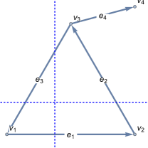
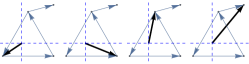
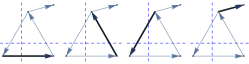
    $x=\left(\right.$ $\left.\right)$ $w=\left(\right.$ $\left.\right)$

Figure 1: A particular graph embedding in $\mathbb{R}^{2}$, along with the components of its vertex vector $x\in(\mathbb{R}^{2})^{4}$ and edge vector $w\in(\mathbb{R}^{2})^{4}$.

In addition to thinking of the vector $x^{k}$ of $k$th coordinates of vertices as a vector in $\mathbb{R}^{\mathbf{v}}$, it will also be useful to think of it as a (scalar) function $x^{k}\colon\thinspace\!\!\{v_{1},\dots,v_{\mathbf{v}}\}\rightarrow\mathbb{R}$ on the vertices of the graph.

By contrast, the vector $w^{k}$ of $k$th coordinates of edge displacements can be interpreted either as a vector in $\mathbb{R}^{\mathbf{e}}$ or as a map $w^{k}\colon\thinspace\!\!\{e_{1},\dots,e_{\mathbf{e}}\}\rightarrow\mathbb{R}$, which we think of as a vector field on the multigraph. Since $\mathbf{G}$ is directed, the sign of $w^{k}(e_{j})$ uniquely determines a direction of flow along edge $e_{j}$.

We now recall the relationship between scalar functions and vector fields on multigraphs. In analogy to vector calculus, it’s standard to define two linear maps between the spaces of functions and vector fields. The gradient field $\operatorname{grad}f$ of a function $f\colon\thinspace\!\!\{v_{1},\dots,v_{\mathbf{v}}\}\rightarrow\mathbb{R}$ is the vector field defined by

$$(\operatorname{grad}f)(e_{j})=f(\operatorname{head}(e_{j}))-f(\operatorname{tail}(e_{j})),$$ (1)

and the divergence $\operatorname{div}u$ of a vector field $u\colon\thinspace\!\!\{e_{1},\dots,e_{\mathbf{e}}\}\rightarrow\mathbb{R}$ is the function

$$(\operatorname{div}u)(v_{i})=\sum_{j=1}^{\mathbf{e}}\begin{cases}-u(e_{j})&\text{if $v_{i}$ is (only) the head of $e_{j}$,}\\ +u(e_{j})&\text{if $v_{i}$ is (only) the tail of $e_{j}$,}\\ 0&\text{if $v_{i}$ is both head and tail of $e_{j}$,}\\ 0&\text{else.}\end{cases}$$

As a matrix, $\operatorname{div}=-B$, where $B$ is the $\mathbf{v}\times\mathbf{e}$ incidence matrix with

$$B_{ij}=\begin{cases}+1&\text{if $v_{i}$ is (only) the head of $e_{j}$,}\\ -1&\text{if $v_{i}$ is (only) the tail of $e_{j}$,}\\ 0&\text{if $v_{i}$ is both head and tail of $e_{j}$,}\\ 0&\text{else.}\end{cases}$$ (2)

Loop edges contribute zero columns, and when there are multiple edges connecting two vertices $B$ will have repeated columns.

On the other hand, $\operatorname{grad}$ is the $\mathbf{e}\times\mathbf{v}$ matrix $B^{T}$. As usual, we will say that $f$ is a potential function for $u$ if $\operatorname{grad}f=u$. We will say $u$ is a conservative vector field if there exists some $f$ so that $\operatorname{grad}f=u$. If $u$ is conservative, there is a one-dimensional family of possible potential functions $f+C$ where $C$ is a constant function on $\mathbf{G}$.

As a subspace of the space of all vector fields, we can characterize the conservative vector fields using a version of the Helmholtz decomposition:

Theorem 2.

The vector space $\mathbb{R}^{\mathbf{e}}$ of vector fields on $\mathbf{G}$ is spanned by a $(\mathbf{v}-1)$-dimensional subspace of conservative vector fields $u=\operatorname{grad}f$ and an orthogonal $(\mathbf{e}-\mathbf{v}+1)$-dimensional space of divergence-free vector fields $u$ with $\operatorname{div}u=0$.

Proof.

The divergence-free fields are by definition $\ker B$. Their orthogonal complement $(\ker B)^{\perp}=\operatorname{im}B^{T}=\operatorname{im}\operatorname{grad}$. Since $\mathbf{G}$ is connected, it is not hard to show directly that $\ker\operatorname{grad}$ is one-dimensional (only the constant functions have no gradient), so $\operatorname{im}\operatorname{grad}$ has dimension $\mathbf{v}-1$. The dimension of $\ker\operatorname{div}$ follows. ∎

Consider the problem of finding a potential function $f$ given a vector field $u\in\operatorname{im}B^{T}$. Since $\ker\operatorname{grad}$ is not empty, this problem is underdetermined: adding something in $\ker\operatorname{grad}$ to any particular solution $f$ still yields a function with $\operatorname{grad}f=B^{T}f=u$. We can define a unique canonical potential function $f$ for $u$ by taking the potential function of minimum norm (among all possible potential functions for $u$).

This minimum norm potential function can be computed conveniently using the Moore–Penrose pseudoinverse. We now recall the definition and some standard properties. The pseudoinverse $A^{+}$ of a matrix $A$ is “as close as possible” to the inverse of a matrix which is not full rank. It may be computed by taking the singular value decomposition $A=U\Sigma V^{T}$ and then defining $A^{+}=V\Sigma^{+}U^{T}$, where $\Sigma^{+}$ is the diagonal matrix whose nonzero entries are the reciprocals of the corresponding nonzero entries in $S$.

Equivalently, the pseudoinverse is defined to be the unique matrix satisfying the four Moore–Penrose conditions:

$$AA^{+}A=A,\quad A^{+}AA^{+}=A^{+},\quad AA^{+}=(AA^{+})^{T},\quad A^{+}A=(A^{+}A)^{T}.\marginpar{\raggedright\tiny\ref{eq:moore penrose conditions}eq:moorepenroseconditions}\ignorespaces\@add@raggedright$$ (3)

It will also be helpful to recall that $AA^{+}$ is the orthogonal projector onto $\operatorname{im}A=(\ker A^{T})^{\perp}$ and $A^{+}A$ is the orthogonal projector onto $\operatorname{im}A^{T}=(\ker A)^{\perp}$ and that $(A^{T})^{+}=(A^{+})^{T}$, so there is no ambiguity in writing $A^{T+}$ for the combination.

It is a standard fact that

Theorem 3.

The smallest $x$ minimizing $\|Ax-b\|^{2}$ is given by $x_{0}=A^{+}b$. Further, $x_{0}\in(\ker A)^{\perp}$, and $Ax_{0}=b$ $\iff$ $b\in\operatorname{im}A$.

Using the theorem, we see that if $u\in\operatorname{im}\operatorname{grad}=\operatorname{im}B^{T}$, then there is a unique potential function $f=B^{T+}u$ in $(\ker B^{T})^{\perp}$. As we noted above, $\ker B^{T}$ is the one-dimensional space of constant functions, so $f\in(\ker B^{T})^{\perp}$ must have $\sum f(v_{i})=0$. It is helpful to note that $B^{T+}u$ is defined for any vector field $u$ (whether or not $u$ is in $\operatorname{im}B^{T}$), though $B^{T}B^{T+}w=u$ if and only if $u\in\operatorname{im}B^{T}$.

The discussion above solves the embedding problem while adroitly sidestepping any mention of the loop constraints themselves. To recover the loops, observe that every loop in the graph has a divergence-free field that flows around it and every vector field perpendicular to that field obeys the corresponding loop constraint. The fields flowing around the loops span $\ker\operatorname{div}$ (for more details, see [Jiang:2011hk]), whose dimension $\mathbf{e}-\mathbf{v}+1$ is exactly the cycle rank of the graph.

III Gaussian random embeddings

With the language above, we see immediately that a collection of scalar functions $x^{1},\dots,x^{d}$ on $\mathbf{G}$ defines an embedding of $\mathbf{G}$ into $\mathbb{R}^{d}$ by letting $x_{i}^{k}$ – the $k$th coordinate of vertex $v_{i}$ – be $x^{k}(v_{i})$. On the other hand, a collection of vector fields $w^{1},\dots,w^{d}$ on $\mathbf{G}$ can be interpreted as a collection of coordinates of edge displacements, but these displacements define an embedding of $\mathbf{G}$ only if $w^{k}\in\operatorname{im}\operatorname{grad}$ for each $k=1,\dots,d$. In this case, the $w$’s define a unique embedding $x^{k}=B^{T+}w^{k}$ with $\sum x_{i}^{k}=0$. We will call such an embedding centered because its center of mass is at the origin.

In analogy to the requirement that the displacements $w$ of a Gaussian random walk are sampled from a standard Gaussian on $(\mathbb{R}^{d})^{\mathbf{e}}$, we make the least restrictive assumption about the distribution of $w^{k}=\operatorname{grad}x^{k}$ that we can:

Definition 4.

A Gaussian random embedding of $\mathbf{G}$ into $\mathbb{R}^{d}$ with $k$th coordinates of the edge displacements $w^{k}$ is defined by the assumption that $w^{k}$ is sampled from a standard normal on $\mathbb{R}^{\mathbf{e}}$ conditioned on the hypothesis that $w^{k}\in\operatorname{im}\operatorname{grad}=\operatorname{im}B^{T}$.

We can immediately compute the covariance matrix of $w^{k}$:

Theorem 5.

If $w$ is the edge vector of a Gaussian random embedding of $\mathbf{G}$ into $\mathbb{R}^{d}$, then the vector $w^{k}$ of $k$th coordinates is distributed as $\mathcal{N}(0,B^{T}B^{T+})=\mathcal{N}(0,B^{+}B)$.

Proof.

To condition on the hypothesis that a multivariate normal is restricted to a linear subspace, we transform the normal by orthogonal projection to that subspace. Using the fact that $B^{T}B^{T+}$ is the (symmetric) orthogonal projector onto $\operatorname{im}B^{T}$ we can compute that the covariance matrix of the projected variable is

$$B^{T}B^{T+}I(B^{T}B^{T+})^{T}=B^{T}B^{T+}=(B^{+}B)^{T}=B^{+}B.$$

This completes the proof. ∎

Given the edge displacements, it is certainly possible to determine the vertex vector of the corresponding centered embedding directly: for the path, the vertex positions are just the partial sums of the displacement vectors. Strictly speaking, this is based on a choice of (the unique) spanning tree for the path graph, but for more complicated multigraph topologies one needs to find a spanning tree before computing the partial sums. It is generally simpler to compute $B^{T+}$ and use the equation $x^{k}=B^{T+}w^{k}$.

Corollary 6.

If $x$ is the vertex vector of a Gaussian random embedding of $\mathbf{G}$ into $\mathbb{R}^{d}$, the vector $x^{k}$ of $k$th coordinates can be constructed by taking $x^{k}=B^{T+}y^{k}$ where $y^{k}$ is distributed as $\mathcal{N}(0,I_{\mathbf{e}})$ on $\mathbb{R}^{\mathbf{e}}$.

Proof.

We know that we can construct $x^{k}$ by taking $x^{k}=B^{T+}w^{k}$, where $w^{k}$ is distributed as $\mathcal{N}(0,B^{T}B^{T+})$ on $\mathbb{R}^{\mathbf{e}}$. In the proof of Theorem 5, we showed that $w^{k}=B^{T}B^{T+}y^{k}$, where $y^{k}$ is distributed as $\mathcal{N}(0,I_{\mathbf{e}})$. Thus $x^{k}=B^{T+}B^{T}B^{T+}y^{k}=B^{T+}y^{k}$ using (3). ∎

We are now going to directly compute the covariance matrix of $x^{k}$. It will help to recall that $BB^{T}=\operatorname{div}\operatorname{grad}$ is also known as the (multi)graph Laplacian $L$. It’s a standard fact that $L=D-A$ where $D$ is the diagonal matrix with entries equal to the degrees of the vertices of the graph and $A$ is the adjacency matrix with $A_{ij}$ recording the number of edges connecting $v_{i}$ and $v_{j}$. For example, if $i=j$ then $A_{ii}$ is twice the number of loops based at $v_{i}$; if $i\neq j$ then $A_{ij}$ is the total number of edges $e_{k}$ with $\{v_{i},v_{j}\}=\{\operatorname{head}(e_{k}),\operatorname{tail}(e_{k})\}$.

Theorem 7.

If $x$ is the vertex vector of a Gaussian random embedding of $\mathbf{G}$ into $\mathbb{R}^{d}$, then the vector $x^{k}$ of $k$th coordinates is distributed as $\mathcal{N}(0,L^{+})$ where $L$ is the graph Laplacian of $\mathbf{G}$. Hence $x^{k}$ may be constructed by

$$x^{k}=(L^{+})^{1/2}y^{k}\marginpar{\raggedright\tiny\ref{eq:square root construction}eq:squarerootconstruction}\ignorespaces\@add@raggedright$$ (4)

where $(L^{+})^{1/2}$ is any symmetric square root of $L^{+}$ and $y^{k}$ is distributed as $\mathcal{N}(0,I_{\mathbf{v}})$ on $\mathbb{R}^{\mathbf{v}}$.

Proof.

For the first part, we know that $x^{k}=B^{T+}y^{k}_{\mathbf{e}}$, where $y^{k}_{\mathbf{e}}$ is distributed as $\mathcal{N}(0,I_{\mathbf{e}})$ on $\mathbb{R}^{\mathbf{e}}$. Therefore $x^{k}$ is a multivariate normal whose covariance matrix is

$$B^{T+}I_{\mathbf{e}}(B^{T+})^{T}=B^{T+}B^{+}=(BB^{T})^{+}=L^{+},$$

using the Moore-Penrose conditions and the fact that $(AA^{T})^{+}=A^{T+}A^{+}$ for any matrix $A$. The construction (4) is justified by the fact that $(L^{+})^{1/2}y^{k}$ is also a multivariate normal with covariance matrix $L^{+}$. To construct a symmetric square root for $L^{+}$, we note that since $L$ is a real symmetric matrix, it has a singular value decomposition in the form $U\Sigma U^{T}$. This means we can let $(L^{+})^{1/2}=U(\Sigma^{+})^{1/2}U^{T}$. ∎

We can sample random conformations of a multigraph $\mathbf{G}$ in two ways: either by generating edge vectors normally and converting to vertex positions as in Corollary 6, or by sampling Gaussians with covariance matrix $L^{+}$ as in Theorem 7. The latter is almost always preferable, since any multigraph with loops has at least as many edges as vertices and the covariance matrix $L^{+}$ only has to be computed once. This, then, gives a powerful computational tool for estimating arbitrary quantities of interest using Monte Carlo integration.

We now do an example. For ring polymers, the graph $\mathbf{G}$ is a cycle graph and the Laplacian is:

$$L=\begin{pmatrix}2&-1&\cdots&\cdots&-1\\ -1&2&-1&\cdots&0\\ 0&-1&2&-1&0\\ \vdots&\vdots&\ddots&\ddots&-1\\ -1&\cdots&\cdots&-1&2\end{pmatrix}$$

A singular value decomposition $L=U\Sigma U^{T}$ is well-known, as $L$ is the discrete Fourier transform. We can write it as

$$\sigma_{j}=4\sin^{2}\frac{\pi j}{\mathbf{v}},\qquad U_{\ell j}=\alpha_{j}\begin{cases}\sin\frac{2\pi j\ell}{\mathbf{v}},&1\leq j<\frac{\mathbf{v}}{2},\\ \cos\frac{2\pi j\ell}{\mathbf{v}},&\frac{\mathbf{v}}{2}\leq j\leq\mathbf{v}.\end{cases}\marginpar{\raggedright\tiny\ref{eq:svd for cycle graph laplacian}eq:svdforcyclegraphlaplacian}\ignorespaces\@add@raggedright$$ (5)

where $\alpha_{j}=\sqrt{\nicefrac{{2}}{{\mathbf{v}}}}$ unless $j=\mathbf{v}$ or $j=\nicefrac{{\mathbf{v}}}{{2}}$ (if $\mathbf{v}$ is even), in which case $\alpha_{j}=\sqrt{\nicefrac{{1}}{{\mathbf{v}}}}$. This allows us to construct a square root $(L^{+})^{1/2}$ whose singular values are $\frac{1}{2}\csc\frac{\pi j}{\mathbf{v}}$ for $1\leq j<\mathbf{v}$ together with a single $0$ corresponding to $\sigma_{\mathbf{v}}=0$ in (5). We note this Fourier description for Gaussian ring polymers was considered by Bloomfield and Zimm [Bloomfield:1966cy] and Eichinger [Eichinger:1972iy].

IV Fourier-type analysis of random graph embeddings

In the proof of Theorem 7, we saw that the vertex vectors of a Gaussian random embedding could be generated by taking

$$x^{k}=U(\Sigma^{+})^{1/2}U^{T}y^{k},\quad y^{k}\text{ distributed as }\mathcal{N}(0,I_{\mathbf{v}}),$$

where $U$ is the matrix of eigenvectors of $L$. Another way to look at this equation is to see that $x^{k}$ is a weighted linear combination of the eigenvectors with random (normal) coefficients where the weights are given by the singular values on the diagonal of $(\Sigma^{+})^{1/2}$:

$$x^{k}=\sum_{\begin{subarray}{c}j\in\{1,\dotsc,\mathbf{v}\}\\ \sigma_{j}\neq 0\end{subarray}}\frac{1}{\sqrt{\sigma_{j}}}u_{j}\cdot y_{j}$$

where each $y_{j}$ is distributed as $\mathcal{N}(0,1)$. It is clear that the eigenfunctions of $L$ with small eigenvalues $\sigma_{j}$ are expected to play a much larger role in determining the vertex vector $x^{k}$ than the eigenfunctions with larger eigenvalues.

We can make this observation precise by recalling a few facts from linear algebra. An optimal rank-$p$ approximation $A_{p}$ to a matrix $A$ with singular value decomposition $U\Sigma V^{T}$ is given by replacing $\Sigma$ with another diagonal matrix $\Sigma_{p}$ keeping a collection $S_{p}$ of the $p$ largest singular values of $\Sigma$ and setting the remaining singular values to zero. We can now define the rank-$p$ approximation to a Gaussian random graph embedding

$$x^{k}_{p}=(L^{+})^{1/2}_{p}y^{k}$$

and note that

$$x^{k}-x^{k}_{p}=((L^{+})^{1/2}-(L^{+})^{1/2}_{p})y^{k}$$

is itself a Gaussian random vector. If $\sigma_{j}^{+}$ are the singular values of $L^{+}$, and $S^{+}_{p}$ is a collection of the $p$ largest $\sigma_{j}^{+}$, then the expected squared norm of this difference vector is

$$\mathcal{E}\left(\left\|x^{k}-x^{k}_{p}\right\|^{2}\right)=\operatorname{tr}\left(L^{+}-L^{+}_{p}\right)=\sum_{\sigma_{j}^{+}\not\in S_{p}}\sigma_{j}^{+}.\marginpar{\raggedright\tiny\ref{eq:p error estimate}eq:perrorestimate}\ignorespaces\@add@raggedright$$ (6)

For the cycle graph, we know from (5) that $\sigma_{j}^{+}=\frac{1}{4}\csc^{2}\frac{\pi j}{\mathbf{v}}$ for $j\in\{1,\dots,\mathbf{v}-1\}$ and $\sigma_{\mathbf{v}}^{+}=0$. Summing the $\sigma_{j}^{+}$ tells us that $\mathcal{E}(\left\|x^{k}\right\|^{2})=\frac{1}{12}(\mathbf{v}^{2}-1)$ and (for $p$ even)

$$$$ (7)