Teaching Machines to Converse

TEACHING MACHINES TO CONVERSE

A DISSERTATION
SUBMITTED TO THE DEPARTMENT OF COMPUTER SCIENCE
AND THE COMMITTEE ON GRADUATE STUDIES
OF STANFORD UNIVERSITY
IN PARTIAL FULFILLMENT OF THE REQUIREMENTS
FOR THE DEGREE OF
DOCTOR OF PHILOSOPHY

Jiwei Li

Abstract

The ability of a machine to communicate with humans has long been associated with the general success of AI. This dates back to Alan Turing’s epoch-making work in the early 1950s, which proposes that a machine’s intelligence can be tested by how well it, the machine, can fool a human into believing that the machine is a human through dialogue conversations. Despite progress in the field of dialogue learning over the past decades, conventional dialog systems still face a variety of major challenges such as robustness, scalability and domain adaptation: many systems learn generation rules from a minimal set of authored rules or labels on top of handcoded rules or templates, and thus are both expensive and difficult to extend to open-domain scenarios. Meanwhile, dialogue systems have become increasingly complicated: they usually involve building many different complex components separately, rendering them unable to accommodate the large amount of data that we have to date.

Recently, the emergence of neural network models the potential to solve many of the problems in dialogue learning that earlier systems cannot tackle: the end-to-end neural frameworks offer the promise of scalability and language-independence, together with the ability to track the dialogue state and then mapping between states and dialogue actions in a way not possible with conventional systems. On the other hand, neural systems bring about new challenges: they tend to output dull and generic responses such as “I don’t know what you are talking about”; they lack a consistent or a coherent persona; they are usually optimized through single-turn conversations and are incapable of handling the long-term success of a conversation; and they are not able to take the advantage of the interactions with humans.

This dissertation attempts to tackle these challenges: Contributions are twofold: (1) we address new challenges presented by neural network models in open-domain dialogue generation systems, which includes (a) using mutual information to avoid dull and generic responses; (b) addressing user consistency issues to avoid inconsistent responses generated by the same user; (c) developing reinforcement learning methods to foster the long-term success of conversations; and (d) using adversarial learning methods to push machines to generate responses that are indistinguishable from human-generated responses; (2) we develop interactive question-answering dialogue systems by (a) giving the agent the ability to ask questions and (b) training a conversation agent through interactions with humans in an online fashion, where a bot improves through communicating with humans and learning from the mistakes that it makes.

Chapter 1 Introduction

By your words you will be justified, and by your words you will be condemned.

Matthew 12:37.

Conversation in the form of languages has always been a trademark of humanity. It is one of the first skills that we humans acquire as kids, and never cease to use throughout our lives, whether a person is ordering a burrito for lunch, taking classes, doing job interviews, discussing the result of an NHL game with friends, or even arguing with others. The significance of conversation/communication also transcends individuals: through conversations, humans can communicate a huge amount of information not only about our surroundings (e.g., asking companions to watch out for the lions in the forest), but about ourselves (e.g., giving orders, talking about personal needs, etc). Such an ability leads to more effective social cooperation, and is a necessity for organizing a larger group of people (e.g., company, troop, etc).

In the field of artificial intelligence, attempts to imitate humans’ ability to converse can be dated back to the early days of AI, and this ability has long been associated with the general success of AI. In his epoch-making paper Turing (1950), Alan Turing proposed a method to test the general intelligence level of a machine, which is widely known as the Turing test or the Imitation game. In the Turing test, a machine is asked to talk with a human. The machine’s intelligence level is decided by how well the machine is able to fool a human evaluator into believing that it, the machine, is a human based on its text responses. If the human evaluator cannot tell the difference between the machine from a human, the machine is said to have passed the Turing test, which signifies a high level of intelligence of an AI.

Ever since the idea of the Turing test was proposed, various attempts have been proposed to pass the test. But we are still far from passing the test. In this section, we will briefly review the systems that have been proposed over the past decades. Specifically, we will discuss three types of dialogue systems: the chit-chat system, the frame-based goal oriented system, and the interactive question-answering (QA) dialogue system. We will discuss the cases where they have been successfully applied, their pros and cons, and why they are still not able to pass the Turing test. The major focus of this thesis is about how to improve the chit-chat system and the interactive question-answering (QA) system.

1.1 A Brief Review of Existing Dialogue Systems

1.1.1 The Chit-chat Style System

A chit-chat-oriented dialogue agent is designed to engage users, comfort them, provide mental support, or just chat with users whichever topic they want to talk about. The bot first needs to understand what its dialogue partner says, and then generate meaningful and coherent responses based on this history. Existing chit-chat systems mostly fall into the following three subcategories: the rule-based systems, the IR-based systems and the generation-based systems, as will be discussed in order below.

The Rule-based Systems

Using rules is one of the most effective ways to generate dialogue utterances. Usually, message inputs are first assessed based on a set of pre-defined rules, e.g., a key-word look-up dictionary, if-else conditions, or more sophisticated machine learning classifiers. After rule conditions are evaluated, relevant actions will be executed, such as outputting an utterance in storage, manipulating the input message or selecting some related historical contexts.

One of the most famous rule-based dialogue systems in history is ELIZA Weizenbaum (1966). ELIZA operates by first searching a keyword existing in the input text from a real human based on a hand-crafted keyword dictionary. If a keyword is found, a rule is applied to manipulate and transform the user’s original input and forwarded back to the user. Otherwise, ELIZA responded either with a generic response or copying one sentence from the dialogue history. Extensions of ELIZA include PARRY Parkinson et al. (1977), also described as ”ELIZA with attitude”, which simulated a patient with schizophrenia. PARRY relies on global variables to keep track of the emotional state, as opposed to ELIZA where responses are generated only based on the previous sentence. A variety of chit-chat systems such as Eugene Goostman, Jabberwacky, Cleverbot, Alice, AIML were proposed after Eliza and PARRY.

ELIZA-style systems are recognized as an important milestone in developing modern dialogue systems. More interestingly, some of the systems seemed to be able to deceive some human evaluators to believe that they were talking with real people in a few specific scenarios Thomas (1995); Colby et al. (1972); Pinar Saygin et al. (2000). On the other hand, their drawbacks are obvious: Rule-based systems predominantly rely on the set of pre-defined rules. The number of these rules skyrockets as the system gets more sophisticated; Rule-based systems do not have the ability to understand human languages, nor do they know how to generate meaningful natural language utterances. They are thus only able to conduct very superficial conversations.

The IR-based Systems

The IR-based methods rely on information retrieval or nearest neighbor techniques Isbell et al. (2000); Jafarpour et al. (2010); Yan et al. (2016a); Al-Rfou et al. (2016); Yan et al. (2016b). Given a history input and a training corpus, the system copies a response from the training corpus. The response selection process is usually based on the combination of the following two criteria: the history associated with the chosen response should be similar to the input dialogue history and the chosen response should be semantically related to the input dialogue history. Various ranking schemes such as semantic relatedness measurements (e.g., vector space models or TF-IDF), page-rank style relatedness propagation models, or personalization techniques can be ensembled into a single ranking function and the response with the highest ranking score will be selected. The pros and cons of the IR-based models are both obvious: on one hand, the models are easy to implement relative to generation-based models; responses are always grammatical (since responses are copied from the training set); and through the manipulation of the ranking function (e.g., adding rules, upweighing or downweighting some particular features), a developer has a relatively good (and direct) control on generating responses that he or she would like to see. But on the other hand, the IR-based models lack the flexibility in handling the diversity of natural languages, the ability to handle important linguistic features such as context structure or coherence, and the capability of discerning the subtle semantic difference between different input contexts.

The Generation-based Systems

The generation-based system generates sentences token by token instead of copying responses from the training set. The task can be formalized as an input-output mapping problem, where given the history dialogue utterances, the system needs to output a coherent and meaningful sequence of words. The task was first studied by Ritter et al. (2011), who frame the response generation task as a statistical machine translation (SMT) problem. The IBM-model Brown et al. (1991) is used to learn the word mapping rules between source and target words (as shown in Figure 1.1) and the phrase-based MT model Chiang (2007) is used for word decoding. The disadvantage of the MT-based system stems not only from the complexity of the phrase-based MT model with many different components built separately, but also from the IBM model’s intrinsic inflexibility in handling the implicit semantic and syntactic relations between message-response pairs: unlike in MT, where there is usually a direct mapping between a word or phrase in the source sentence and another word or phrase in the target sentence, in response generation, the mapping is mostly beyond the word level, and requires the semantic of the entire sentence. Due to this reason, the MT-based system is only good at handling the few cases in which word-level mapping is very clear as in Figure 1.1, but usually fail to tackle the situations once the semantic of an input sentence gets complex, sometimes outputting incoherent, or even ungrammatical responses. Furthermore, the MT-based system lacks the ability to leverage information in the multi-context situation.

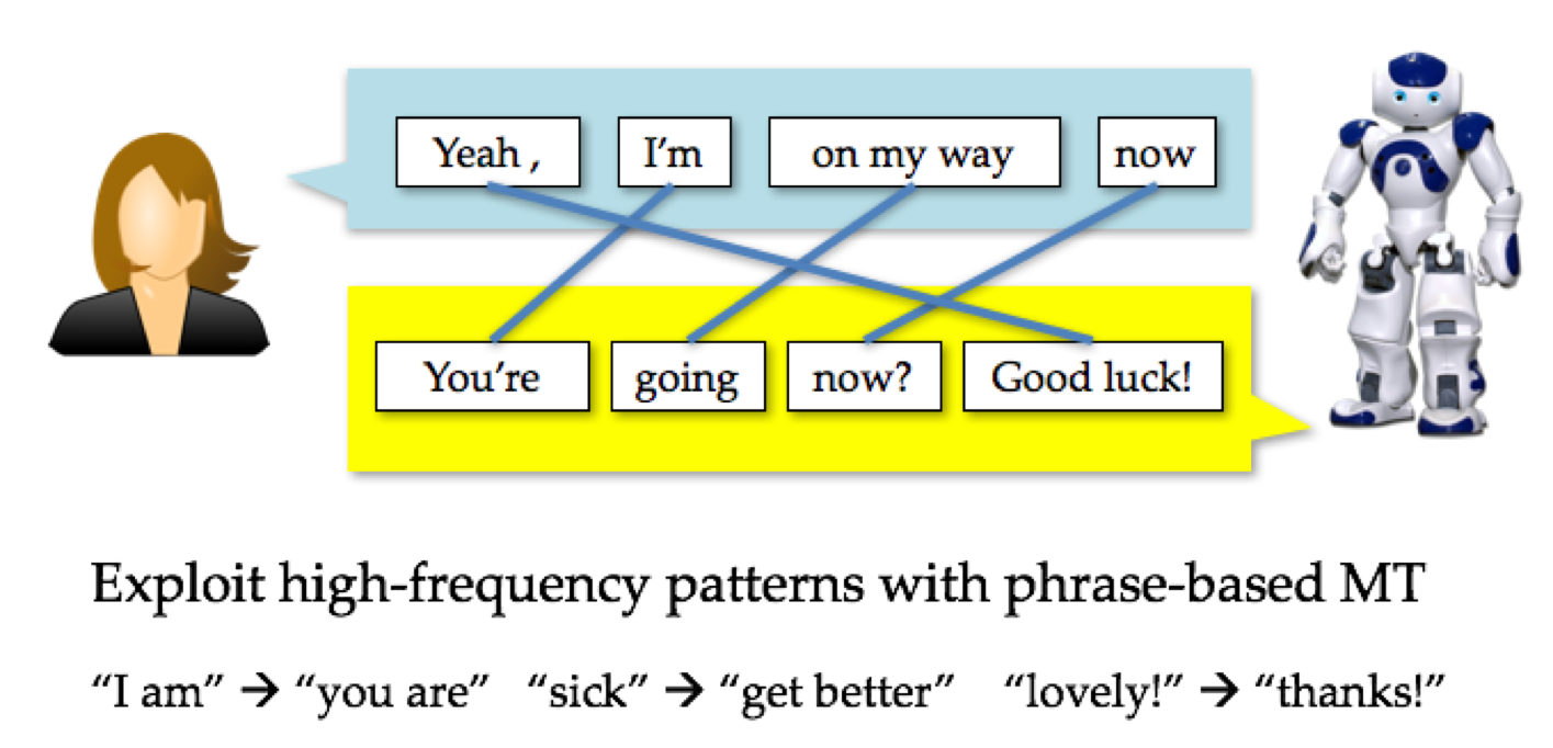
Figure 1.1: Word alignments between messages and responses using the IBM model. Image courtesy of Michel Galley.

Recent progress in SMT, which stems from the use of neural language models Mikolov et al. (2010); Kalchbrenner and Blunsom (2013); Vaswani et al. (2013) and neural sequence-to-sequence generation models (Seq2Seq) Sutskever et al. (2014); Bahdanau et al. (2014); Cho et al. (2014); Luong et al. (2015b, 2014); Luong and Manning (2016) have inspired a variety of attempts to extend neural techniques to response generation Sordoni et al. (2016); Ghazvininejad et al. (2017); Mostafazadeh et al. (2017); Serban et al. (2017b, 2016a, 2016b, a). Neural models offer the promise of scalability and language-independence, together with the capacity to implicitly learn semantic and syntactic relations between pairs, and to capture contextual dependencies in a way not possible with conventional SMT approaches or IR-based approaches.

Due to these advantages, neural generation models are able generate more specific, coherent, and meaningful dialogue responses. On the other hand, a variety of important issues still remain unsolved: current systems tend to generate plain and dull responses such as “i don’t know what you are talking about”, which discourages the conversation; it is hard to endow a dialogue system with a consistent element of identity or persona (background facts or user profile), language behavior or interaction style; current systems usually focus on single-turn conversations, or two-turns at most, since it is hard to give the system a long-term planning ability to conduct multi-turn conversations that flow smoothly, coherently, and meaningfully. This thesis tries to address these issues.

1.1.2 The Frame-based Dialogue Systems

The frame-based system, first proposed by Bobrow et al. (1977), models conversations guided by frames, which represent the information at different levels within a conversation. For example, in a conversation about plane ticket booking, frames include important aspects such as Person, Traveling Date, Destination, TimeRange of the flight, etc. Frames of a conversation define the aspects that the conversation should cover and the relations (e.g., one frame is a prototype of another) between frames define how conversations should flow Walker and Whittaker (1990); Seneff (1992); Chu-Carroll and Brown (1997); San-Segundo et al. (2001); Seneff (2002).

The simplest frame-based system is a finite-state machine, which asks the user a series of pre-defined questions based on the frames, and moves on to the next question if a customer provides an answer, and ignores anything from the customer if the response is not an answer. More complicated architectures allow the initiative of the conversation between the system and the user to shift at various points. These systems rely on a pre-defined frame and asks the user to fill slots in the frame, where a task is completed if all frame slots have been filled . The limitation of the frame-based system is that the dialogue generation process is completely guided by what needs to fill the slots. The system doesn’t have the ability to decide the progress or the state of the conversation, e.g., whether the customer has rejected a suggestion, asked a question, or whether the system now needs to give suggestions or ask clarification questions, etc, and is thus not able to take a correct action given the progress so far.

To overcome these drawbacks, more sophisticated state-based dialogue models Nagata and Morimoto (1994); Reithinger et al. (1996); Warnke et al. (1997); Stolcke et al. (2000); Allen et al. (2001) were designed. The state-based dialogue system is based on two key concepts, dialogue state, which denotes the progress of current conversation, including context information, intentions of the speakers, etc, and dialogue acts, which characterize the category of a dialogue utterance. The choice of a dialogue act is based on the dialogue state the conversation is currently in, and the key component of this system is to learn the optimal mapping between a state and an action to take, which is able to maximize dialogue success. Reinforcement learning methods such as MDPs or POMDPs are widely used to learn such mappings based on external rewards that define dialogue success Young (2000, 2002); Lemon et al. (2006); Williams and Young (2007); Young et al. (2010, 2013). Recent advances in neural network models provide with more power and flexibility in keeping track of dialogue states and modeling the mapping between the dialogue states and utterances to generate Wen et al. (2015); Mrkšić et al. (2015); Su et al. (2015); Wen et al. (2016b, a); Su et al. (2016a, b); Wen et al. (2017).

Frame-based systems have succeeded in a variety of applications such as booking flight tickets, reserving restaurants, etc, some of which have already been in use in our everyday life. The biggest advantages of frame-based system are that the goal of the system is explicitly defined and that the pre-defined frames give a very clear guidance on how a conversation should proceed. On the other hand, its limitation is clear: frame-based systems heavily rely on sophisticated hand-crafted patterns or rules, and these rules are costly; rules have to be rebuilt when the system is adapted to a new domain or an old domain changes, making the system difficult to scale up. More broadly, it does not touch the complex linguistic features involved in human conversations, such as context coherence, word usage (both semantic and syntactic), personalization, and are thus not able to capture the complexity and the intriguing nature of humans’ conversation.

In this thesis, we do not focus on frame-based systems.

1.1.3 The Question-Answering (QA) Based Dialogue System

Another important dialogue system is the factoid QA-based dialogue system, which is closely related to developing automated personal assistant systems such as Apple’s Siri. A dialogue agent needs to answer customers’ questions regarding different topics such as weather conditions, traffic congestion, news, stock prices, user schedules, retail prices, etc D’agostino (1993); Modi et al. (2005); Myers et al. (2007); Berry et al. (2011), either given a database of knowledge Dodge et al. (2016); Bordes et al. (2015); Weston (2016), or from texts Hermann et al. (2015); Weston et al. (2016); Weston (2016). The QA based dialogue system is thus related to a wide range of work in text-based or knowledge-base based question answering, e.g., Hirschman and Gaizauskas (2001); Clarke and Terra (2003); Maybury (2008); Berant et al. (2013); Iyyer et al. (2014); Rajpurkar et al. (2016) and many many others. The key difference between a QA-based dialogue system and a factoid QA-system is that the QA-based dialogue system is interactive Rieser and Lemon (2009): instead of just having to answer one single question, the QA-based system needs the ability to handle a diverse category of interaction-related issues such as asking for question clarification Stoyanchev et al. (2013, 2014), adapting answers given a human’s feedback Rieser and Lemon (2009), self-learning when encountering new questions or concepts Purver (2006), etc. To handle these issues, the system needs to take proper actions based on the current conversation state, which resembles the key issue addressed in the state-based dialogue system.

How a bot can be smart about interacting with humans, and how to improve itself through these interactions are not sufficiently studied. For example, asking for question clarification is only superficially touched in Stoyanchev et al. (2013, 2014) for cases where some important tokens are not well transcribed from the speech, for example,

A: When did the problems with [power] start?

B: The problem with what?

A: Power.

But important scenarios such as what if there is an out-of-vocabulary word in the original question, how a bot can ask for hints, and more importantly, how a bot can be smart about deciding whether, when and what to ask have rarely been studied. Another important aspect in developing interactive agent that is missing from existing literature is that a good agent should have the ability to learn from the online feedback: adapting its model when making mistakes and reinforcing the model when a human’s feedback is positive. This is particularly important in the situation where the bot is initially trained in a supervised way on a fixed synthetic, domain-specific or pre-built dataset before release, but will be exposed to a different environment after release (e.g., more diverse natural language utterance usage when talking with real humans, different distributions, special cases, etc.). There hasn’t been any work discussing how a bot effectively improve itself from online feedback by accommodating various feedback signals. This thesis tries to address these questions.

1.2 Thesis Outline

In this dissertation, we mainly address problems involved in the chit-chat system and the interactive QA system. First, we explore how to build an engaging chit-chat style dialogue system that is able to conduct interesting, meaningful, coherent, consistent, and long-term conversation with humans. More specially, for the chit-chat system, we (a) use mutual information to avoid dull and generic responses Li et al. (2016a, c, 2017c); (b) address user consistency issues to avoid inconsistent responses from the same user Li et al. (2016b); (c) develop reinforcement learning methods to foster the long-term success of conversations Li et al. (2016d); and (d) use adversarial learning methods to generate machine responses that are indistinguishable from human-generated responses Li et al. (2017d);

Second, we explore how a bot can best improve itself through the online interactions with humans that makes a chatbot system trully interactive. We develop interactive dialogue systems for factoid question-answering: (a) we design an environment that provides the agent the ability to ask humans questions and to learn when and what to ask Li et al. (2017b); (b) we train a conversation agent through interaction with humans in an online fashion, where a bot improves through communicating with humans and learning from the mistakes that it makes Li et al. (2017a).

We start off by providing background knowledge on Seq2Seq models, memory network models and policy gradient reinforcement learning models in Chapter 2. The aforementioned four problems for the chit-chat style dialogue generation systems will be detailed in Chapters 3,4,5,6, and the two issues with the interactive QA system will be detailed in Chapters 7 and 8. We conclude this dissertation and discuss future avenue for chatbot development in Chapter 9.

1.2.1 Open-Domain Dialogue Generation

Mutual Information to Avoid Generic Responses

An engaging response generation system should be able to output grammatical, coherent responses that are diverse and interesting. In practice, however, neural conversation models exhibit a tendency to generate dull, trivial or non-committal responses, often involving high-frequency phrases along the lines of I don’t know or I’m OK Sordoni et al. (2016); Serban et al. (2015); Vinyals and Le (2015). This behavior is ascribed to the relative frequency of generic responses like I don’t know in conversational datasets, in contrast with the relative sparsity of other, more contentful or specific alternative responses. It appears that by optimizing for the likelihood of outputs/targets/responses given inputs/sources/messages, neural models assign high probability to “safe” responses. The question is how to overcome the neural models’ predilection for the commonplace. Intuitively, we want to capture not only the dependency of responses on messages, but also the inverse, the likelihood that a message will be provided to a given response. Whereas the sequence I don’t know is of high probability in response to most question-related messages, the reverse will generally not be true, since I don’t know can be a response to everything, making it hard to guess the original input question.

We propose to capture this intuition by using Maximum Mutual Information (MMI), as an optimization objective that measures the mutual dependence between inputs and outputs, as opposed to the uni-directional dependency from sources to targets in the traditional MLE objective function. We present practical training and decoding strategies for neural generation models that use MMI as objective function. We demonstrate that using MMI results in a clear decrease in the proportion of generic response sequences, and find a significant performance boost from the proposed models as measured by BLEU Papineni et al. (2002) and human evaluation. This chapter is based on the following three papers: Li et al. (2016a, c, 2017c), and will be detailed in Section 3.

Addressing the Speaker Consistency Issue

An issue that stands out with current dialogue systems is the lack of speaker consistency: if a human asks a bot a few questions, there is no guarantee that answers from the bot are consistent. This is because responses are selected based on likelihood assigned by the pre-trained model, which does not have the ability to model speaker consistency.

In Li et al. (2016b), we address the challenge of consistency and how to endow data-driven systems with the coherent “persona” needed to model human-like behavior, whether as personal assistants, personalized avatar-like agents, or game characters. For present purposes, we will define persona as the character that an artificial agent, as actor, plays or performs during conversational interactions. A persona can be viewed as a composite of elements of identity (background facts or user profile), language behavior, and interaction style. A persona is also adaptive, since an agent may need to present different facets to different human interlocutors depending on the demands of the interaction. We incorporate personas as embeddings and explore two persona models, a single-speaker Speaker Model and a dyadic Speaker-Addressee Model, within the Seq2Seq framework. The Speaker Model integrates a speaker-level vector representation into the target part of the Seq2Seq model. Analogously, the Speaker-Addressee model encodes the interaction patterns of two interlocutors by constructing an interaction representation from their individual embeddings and incorporating it into the Seq2Seq model. These persona vectors are trained on human-human conversation data and used at test time to generate personalized responses. Our experiments on an open-domain corpus of Twitter conversations and dialog datasets comprising TV series scripts show that leveraging persona vectors can improve relative performance up to $20\%$ in BLEU score and $12\%$ in perplexity, with a commensurate gain in consistency as judged by human annotators. This chapter is based on the following paper: Li et al. (2016b), and will be detailed in Section 4.

Fostering Long-term Dialogue Success

Current dialogue generation models are trained by predicting the next single dialogue turn in a given conversational context using the maximum-likelihood estimation (MLE) objective function. However, this does not mimic how we humans talk. In everyday conversations from a human, each human dialogue episode consists tens of, or even hundreds of dialogue turns rather than only one turn; humans are smart in controlling the informational flow in a conversation for the long-term success of the conversation. Current models’ incapability of handling this long-term success result in repetitive and generic responses.

We need a conversation framework that has the ability to (1) integrate developer-defined rewards that better mimic the true goal of chatbot development and (2) model the long-term influence of a generated response in an ongoing dialogue. To achieve these goals, we draw on the insights of reinforcement learning, which have been widely applied in MDP and POMDP dialogue systems. We introduce a neural reinforcement learning (RL) generation method, which can optimize long-term rewards designed by system developers. Our model uses the encoder-decoder architecture as its backbone, and simulates conversation between two virtual agents to explore the space of possible actions while learning to maximize expected reward. We define simple heuristic approximations to rewards that characterize good conversations: good conversations are forward-looking Allwood et al. (1992) or interactive (a turn suggests a following turn), informative, and coherent. The parameters of an encoder-decoder RNN define a policy over an infinite action space consisting of all possible utterances. The agent learns a policy by optimizing the long-term developer-defined reward from ongoing dialogue simulations using policy gradient methods Williams (1992), rather than the MLE objective defined in standard Seq2Seq models.

Our model thus integrates the power of Seq2Seq systems to learn compositional semantic meanings of utterances with the strengths of reinforcement learning in optimizing for long-term goals across a conversation. Experimental results demonstrate that our approach fosters a more sustained dialogue and manages to produce more interactive responses than standard Seq2Seq models trained using the MLE objective. This chapter is based on the following paper: Li et al. (2016d), and will be detailed in Section 5.

Adversarial Learning for Dialogue Generation

Open domain dialogue generation aims at generating meaningful and coherent dialogue responses given input dialogue history. Current systems approximate such a goal using imitation learning or variations of imitation learning: predicting the next dialogue utterance in human conversations given the dialogue history. Despite its success, many issues emerge resulting from this over-simplified training objective: responses are highly dull and generic, repetitive, and short-sighted.

Solutions to these problems require answering a few fundamental questions: what are the crucial aspects that define an ideal conversation, how can we quantitatively measure them, and how can we incorporate them into a machine learning system: A good dialogue model should generate utterances indistinguishable from human dialogues. Such a goal suggests a training objective resembling the idea of the Turing test Turing (1950). We borrow the idea of adversarial training Goodfellow et al. (2014) in computer vision, in which we jointly train two models, a generator (which takes the form of the neural Seq2Seq model) that defines the probability of generating a dialogue sequence, and a discriminator that labels dialogues as human-generated or machine-generated. This discriminator is analogous to the evaluator in the Turing test. We cast the task as a reinforcement learning problem, in which the quality of machine-generated utterances is measured by its ability to fool the discriminator into believing that it is a human-generated one. The output from the discriminator is used as a reward to the generator, pushing it to generate utterances indistinguishable from human-generated dialogues.

Experimental results demonstrate that our approach produces more interactive, interesting, and non-repetitive responses than standard SEQ2SEQ models trained using the MLE objective function. This chapter is based on the following paper: Li et al. (2017d), and will be detailed in Section 6.

1.2.2 Building Interactive Bots for Factoid Question-Answering

Learning by Asking Questions

For current chatbot systems, when the bot encounters a confusing situation such as an unknown surface form (phrase or structure), a semantically complicated sentence or an unknown word, the agent will either make a (usually poor) guess or will redirect the user to other resources (e.g., a search engine, as in Siri). Humans, in contrast, can adapt to many situations by asking questions: when a student is asked a question by a teacher, but is not confident about the answer, they may ask for clarification or hints. A good conversational agent should have this ability to interact with a customer.

Here, we try to bridge the gap between how a human and an end-to-end machine learning system by equipping the bot with the ability to ask questions. We identify three categories of mistakes a bot can make during dialogue : (1) the bot has problems understanding the surface form of the text of the dialogue partner, e.g., the phrasing of a question; (2) the bot has a problem with reasoning, e.g., it fails to retrieve and connect the relevant knowledge to the question at hand; (3) the bot lacks the knowledge necessary to answer the question in the first place – that is, the knowledge sources the bot has access to do not contain the needed information. All the situations above can be potentially addressed through interaction with the dialogue partner. Such interactions can be used to learn to perform better in future dialogues. If a human bot has problems understanding a teacher’s question, they might ask the teacher to clarify the question. If the bot doesn’t know where to start, they might ask the teacher to point out which known facts are most relevant. If the bot doesn’t know the information needed at all, they might ask the teacher to tell them the knowledge they’re missing, writing it down for future use.

We explore how a bot can benefit from interaction by asking questions in both offline supervised settings and online reinforcement learning settings, as well as how to choose when to ask questions in the latter setting. In both cases, we find that the learning system improves through interacting with users. This chapter is based on the following paper: Li et al. (2017b), and will be detailed in Section 7.

Dialogue Learning with Human-in-the-Loop

A good conversational agent should have the ability to learn from the online feedback from a teacher: adapting its model when making mistakes and reinforcing the model when the teacher’s feedback is positive. This is particularly important in the situation where the bot is initially trained in a supervised way on a fixed synthetic, domain-specific or pre-built dataset before release, but will be exposed to a different environment after release (e.g., more diverse natural language utterance usage when talking with real humans, different distributions, special cases, etc.). Most recent research has focused on training a bot from fixed training sets of labeled data but seldom on how the bot can improve through online interaction with humans. Human (rather than machine) language learning happens during communication (Bassiri, 2011; Werts et al., 1995), and not from labeled datasets, hence making this an important subject to study.

Here, we explore this direction by training a bot through interaction with teachers in an online fashion. The task is formalized under the general framework of reinforcement learning via the teacher’s (dialogue partner’s) feedback to the dialogue actions from the bot. The dialogue takes place in the context of question-answering tasks and the bot has to, given either a short story or a set of facts, answer a set of questions from the teacher. We consider two types of feedback: explicit numerical rewards as in conventional reinforcement learning, and textual feedback which is more natural in human dialogue, following (Weston, 2016). We consider two online training scenarios: (i) where the task is built with a dialogue simulator allowing for easy analysis and repeatability of experiments; and (ii) where the teachers are real humans using Amazon Mechanical Turk.

We explore important issues involved in online learning such as how a bot can be most efficiently trained using a minimal amount of teacher’s feedback, how a bot can harness different types of feedback signal, how to avoid pitfalls such as instability during online learing with different types of feedback via data balancing and exploration, and how to make learning with real humans feasible via data batching. Our findings indicate that it is feasible to build a pipeline that starts from a model trained with fixed data and then learns from interactions with humans to improve itself. This chapter is based on the following paper: Li et al. (2017a), and will be detailed in Section 8.

Chapter 2 Background

In this chapter, we will detail background knowledge on three topics, namely, Seq2Seq models, memory networks, and policy gradient methods of reinforcement learning.

2.1 Sequence-to-Sequence Generation

Seq2Seq models can be viewed as a basic framework for generating a target sentence based on source inputs, which can be adapted to a variety of natural language generation tasks, for example, generating a French sentence given an English sentence in machine translation; generating a response given a source message in response generation; generating an answer given a question in question-answering; generating a short summary given a document in summarization, etc.

We will first go through the basics of language models, recurrent neural networks, and the Long Short-term Memory, which can be viewed as the fundamental components of Seq2Seq models. Then we will detail the basic structure of a Seq2Seq model. Finally, we will talk about algorithmic variations of Seq2Seq models, such as attention mechanism.

2.1.1 Language Modeling

Language modeling is a task of predicting which word comes next given the preceding words, which an important concept in natural language processing. The concept of language modeling can be dated back to the epoch-making work Shannon (1951) of Claude Shannon, who considered the case in which a string of input symbols is considered one by one, and the uncertainty of the next is measured by counting how difficult it is to guess. More formally, language modeling defines the probability of a sequence (of words) by individually predicting each word within the sequence given all the preceding words (or history): $y=y_{1},y_{2},....,y_{N}$, where $y_{t}$ denotes the word token at position $t$ and $N$ denotes the number of tokens in $y$

$$p(y)=\prod_{t=1}^{t=N}p(y_{t}|y_{1},y_{2},...,y_{t-1})$$ (2.1)

where $p(y_{t}|y_{1},y_{2},...,y_{t-1})$ denotes the conditional probability of seeing word $y_{t}$ given that all its preceding words, i.e., $y_{1},y_{2},...,y_{t-1}$. n-gram language models have been widely used, which approximate the history with $n-1$ preceding words. The conditional probability is then estimated from relative frequency counts: count the number of times that we see $y_{t-n+1},...,y_{t-1}$ and count the number of times it is followed by $y_{t}$:

$$p(y_{t}|y_{1},y_{2},...,y_{t-1})=\frac{C(y_{t-n+1},...,y_{t-1},y_{t})}{C(y_{t-n+1},...,y_{t-1})}$$ (2.2)

A variation of algorithmic variations (e.g., smoothing techniques, model compressing techniques) have been proposed Kneser and Ney (1995); Rosenfeld (2000); Stolcke et al. (2002); Teh (2006); Federico et al. (2008); Federico (1996); Chen and Goodman (1996); Bacchiani et al. (2004); Brants et al. (2007); Church et al. (2007). N-gram language modeling comes with the merit of easy and fast implementation, but suffers from a number of severe issues such as data sparsity, poor generalization to unseen words, humongous space requirement for model storage and the incapability to handle long term dependency since the model is only able to consider 4-6 context words.

Neural language modeling (NLM) offers an elegant way to handle the issues of data sparsity and the incapability to consider more context words. It was first proposed in Bengio et al. (2003) and improved by many others Morin and Bengio (2005); Mnih and Hinton (2009); Mnih and Teh (2012); Le and Mikolov (2014); Mikolov et al. (2010); Graves (2013); Kim et al. (2016). In NLM, each word is represented with a distinct $K$-dimensional distributed vector representation. Semantically similar words occupy similar positions in the vector space, which significantly alleviate the data sparsity issue. NLM takes as input the vector representations of context words and maps them to a vector representation:

$$h_{t-1}=f(y_{1},y_{2},...,y_{t-1})$$ (2.3)

where $f$ denotes the mapping function, which is usually a feed-forward neural network model such as recurrent neural nets or convolutional neural nets, as will be detailed in the following subsection. The conditional probability distribution of predicting word $y_{t}$ given the history context is then given as follows:

$$p(y_{t}|y_{1},y_{2},...,y_{t-1}) =p(y_{t}|h_{t-1})$$ (2.4)

$$s_{t} =W[y_{t},:]\cdot h_{t-1}$$

$$p(y_{t}|h_{t-1}) =\operatorname{softmax}(s_{t})$$

where the weight matrix $W\in\mathbb{R}^{V\times K}$, with $V$ the vocabulary size and $K$ being the dimensionality of the word vector representation. $W[y_{t},:]$ denotes the $y_{t}$ th row of the matrix. The softmax function maps the scalar vector $s_{t}$ into a vector of probability distribution as follows:

$$\operatorname{softmax}(s_{t})=\frac{\exp{(s_{t})}}{\sum_{s\in V}\exp{(s)}}$$ (2.5)

Since the dimensionality of the context is immune to the change of context length, theoretically, NLM is able to accommodate infinite number of context words without having to store all distinct n-grams.

2.1.2 Recurrent Neural Networks

Recurrent neural networks (RNN) are a neural network architecture which is specifically designed to handle sequential data. It was historically used to handle time sequential data Elman (1990); Funahashi and Nakamura (1993), and have been successfully applied to language processing Mikolov et al. (2010, 2011); Mikolov (2012); Mikolov and Zweig (2012). Given a sequence of word tokens $\{y_{1},y_{2},...,y_{N}\}$, where each word $y_{t},t\in[1,N]$ is associated with a K-dimensional vector representation $x_{t}$. RNN associates each time step $t$ with a hidden vector representation $h_{t}$, which can be thought of as a representation that embeds all information of previous tokens, i.e., $\{y_{1},y_{2},...,y_{t}\}$. $h_{t}$ is obtained using a function $g$ that combine the previously built presentation for the previous time-step t-1, denoted as $h_{t-1}$, and the representation for the word of current time-step $x_{t}$:

$$h_{t}=g(h_{t-1},x_{t})$$ (2.6)

The function $g$ can take different forms, with the simplistic one being as follows:

$$g(h_{t-1},x_{t})=\sigma(W_{hh}\cdot h_{t-1}+W_{xh}\cdot x_{t})$$ (2.7)

where $W_{hh},W_{xh}\in\mathbb{R}^{K\times 2K}$. Popular choices of $\sigma$ are non-linear functions such as sigmoid, $\tanh$ or ReLU. From Equ. 2.7, we can see that the dimensionality of $h_{t}$ is constant for different $t$.

2.1.3 Long Short Term Memory

Two serve issues problems with RNNs are the gradient exploding problem and the gradient vanishing problem Bengio et al. (1994), where gradient exploding refers to the situation where the gradients become very large when the error from the training objective function is backpropagated over time, and gradient vanishing refers to the situation where the gradients approaches zero when the training error is backpropagated over a few time-steps. These two issues render RNN models incapable of capturing the long-term dependency for long sequences.

One of the most effective ways to alleviate these problem is the Long Short Term Memory model, LSTM for short, first introduced in Hochreiter and Schmidhuber (1997), and adapted , used, and further explored by many others Graves and Schmidhuber (2005, 2009); Chung et al. (2014); Tai et al. (2015); Xu et al. (2015); Kalchbrenner et al. (2016); Cheng et al. (2016); Oord et al. (2016); Jozefowicz et al. (2015); Greff et al. (2017); Zaremba et al. (2014). The key idea of LSTMs is to associate each time step with different types of gates, and these gates provide flexibility in controlling informational flow: to control how much information the current RNN wants to preserve through forget gates; to control how much information a RNN want to receive through the input of current time-step through input gates; and how much information a RNN wants to output to the next time-step through output gates.

More formally, given a sequence of inputs $\{y_{1},y_{2},...,y_{N}\}$, where each word $y_{t}$ is associated with a $K$-dimensional vector representation $x_{t}$, an LSTM associates each time step with an input gate, a memory gate and an output gate, respectively denoted as $i_{t}$, $f_{t}$, and $o_{t}$. $c_{t}$ is the cell state vector at time $t$, and $\sigma$ denotes the sigmoid function. Then, the vector representation $h_{t}$ for each time step $t$ is given by:

$$i_{t}=\sigma(W_{i}\cdot[h_{t-1},x_{t}])$$ (2.8)

$$f_{t}=\sigma(W_{f}\cdot[h_{t-1},x_{t}])$$ (2.9)

$$o_{t}=\sigma(W_{o}\cdot[h_{t-1},x_{t}])$$ (2.10)

$$l_{t}=\tanh(W_{l}\cdot[h_{t-1},x_{t}])$$ (2.11)

$$c_{t}=f_{t}\circ c_{t-1}+i_{t}\circ l_{t}$$ (2.12)

$$h_{t}=o_{t}\cdot\tanh(c_{t})$$ (2.13)

where $W_{i}$, $W_{f}$, $W_{o}$, $W_{l}\in\mathbb{R}^{K\times 2K}$, and $\circ$ denotes the pairwise dot between two vectors. Again, as in RNNs, $h_{t}$ is used as a representation for the partial sequence $\{y_{1},y_{2},...,y_{t}\}$.

2.1.4 Sequence-to-Sequence Generation

The Seq2Seq model can be viewed as an extension of language model, where $y$ is the target sentence, and the prediction of current word $y_{t}$ in $y$ depends not only on all preceding words $\{y_{1},y_{2},...,y_{t-1}\}$, but also on a source input $x$. Each sentence concludes with a special end-of-sentence symbol EOS. For example, in French-English translation, the English word to predict not only depends on all the preceding words, but also depend on the original French input; as another example, the following word in a dialogue response depends both on preceding words in the response and the message input. The Seq2Seq model was first proved to yield good performance in machine translation Sutskever et al. (2014); Bahdanau et al. (2014); Cho et al. (2014); Luong et al. (2015b, 2014); Luong and Manning (2016); Sennrich et al. (2015); Kim and Rush (2016); Wiseman and Rush (2016); Britz et al. (2017); Wu et al. (2016), and has been successfully extended to multiple natural language generation tasks such as text summarization Rush et al. (2015); See et al. (2017); Chopra et al. (2016); Nallapati et al. (2016); Zeng et al. (2016), parsing Luong et al. (2015a); Vinyals et al. (2015); Jia and Liang (2016), image caption generation Chen and Lawrence Zitnick (2015); Xu et al. (2015); Karpathy and Fei-Fei (2015); Mao et al. (2014), etc.

More formally, in Seq2Seq generation tasks, each input $x=\{x_{1},x_{2},...,x_{n_{x}}\}$ is paired with a sequence of outputs to predict: $y=\{y_{1},y_{2},...,y_{n_{y}}\}$. A Seq2Seq generation model defines a distribution over outputs and sequentially predicts tokens using a softmax function:

$$p(y|x) =\prod_{t=1}^{n_{y}}p(y_{t}|y_{1},y_{2},...,y_{t-1},x)$$ (2.14)

By comparing Eq.2.14 with the conditional probability of language modeling in Eq. 2.1, we can see that the only difference between them is the additional consideration of the source input $x$.

More specifically, a standard Seq2Seq model consists of two key components, a encoder, which maps the source input $x$ to a vector representation, and a decoder, which generates an output sequence based on the source sentence. Both the encoder and the decoder are multi-layer LSTMs. To enable the encoder to access information from the encoder, the last state memory of the encoder is passed to the decoder as the initial memory state, based on which words are sequentially predicted using a softmax function. Commonly, input and output use different LSTMs with separate compositional parameters to capture different compositional patterns.

Training

Given a training dataset where each target $y$ is paired with a source $x$, the learning objective is to minimize the negative log-likelihood of predicting each word in the target $y$ given the source $x$:

$$J=-\sum_{t=1}^{t=n_{y}}\log p(y_{t}|x,y_{1},y_{2},...,y_{t-1})$$ (2.15)

Parameters including word embeddings and LSTMs’ parameters are usually initialized from a uniform distribution and learned and optimized using mini-batch stochastic gradient decent with momentum. Gradient clipping is usually adopted by scaling gradients when the norm exceeded a threshold to avoid gradient explosion. Learning rate is gradually decreased towards the end of training.

Testing

Using a pre-trained model, we need to generate an output sequence $y$ given a new input $x$. The problem can be formalized as a standard search problem: generating a sequence of tokens with the largest probability assigned by the pre-trained model, where standard greedy search and beam search can be immediately used. For greedy search, at each time step, the model picks the word with largest probability. For beam search with beam size $K$, for each time-step, we expand each of the $K$ hypotheses by $K$ children, which gives at $K\times K$ hypotheses. We keep the top $K$ ones, delete the others and move on to the next time-step.

During decoding, the algorithm terminates when an EOS token is predicted. At each time step, either a greedy approach or beam search can be adopted for word prediction. Greedy search selects the token with the largest conditional probability, the embedding of which is then combined with preceding output to predict the token at the next step.

2.1.5 Attention Mechanisms

The standard version Seq2Seq model only uses the source representation once, which is through initializing the decoder LSTM using the final state of the encoder LSTM. It is challenging to handle long-term dependency using such a mechanism: the hidden state of the decoder LSTM changes over time as new words are decoded and combined, which dilutes the influence from the source sentence.

One effective way to address such an issue is using attention mechanisms Bahdanau et al. (2014); Xu et al. (2015); Jean et al. (2015); Luong et al. (2015b); Mnih et al. (2014); Chorowski et al. (2014). The attention mechanisms adopt a look-back strategy by linking the current decoding stage with each input time-step in an attempt to consider which part of the input is most responsible for the current decoding time-step.

More formally, suppose that each time-step of the source input is associated with a vector representation $h_{i},i\in[1,n_{x}]$ computed by LSTMs, where $n_{x}$ denotes the length of the source sentence. $h_{i}\in\mathbb{R}^{K\times 1}$. At the current decoding time-step $t$, attention models would first link the current step decoding information $h_{t-1}\in\mathbb{R}^{K\times 1}$ with each of the input time step, characterized by a strength indicator $v_{i}$:

$$v_{i}=h_{t-1}^{T}\cdot h_{i}$$ (2.16)

Other than using the dot product to compute the strength indicator $v_{i}$, many other mechanisms have been used such as vector concatenation, where $v_{i}=\tanh(W\cdot[h_{t-1},h_{i}])$, $W\in\mathbb{R}^{K\times 2K}$, or the general dot-product mechanism, where $v_{i}=h_{t-1}^{T}\cdot W\cdot h_{i}$, $W\in\mathbb{R}^{K\times K}$, as detailedly explored in Luong et al. (2015b). $v_{t}$ is then normalized to a probabilistic value $a_{i}$ using a softmax function:

$$a_{i}=\frac{\exp{(v_{i})}}{\sum_{i^{\prime}}\exp(v_{i^{\prime}})}$$ (2.17)

The context vector $ct_{t-1}$ is the weighted sum of hidden memories on the source side:

$$ct_{t-1}=\sum_{i=1}^{i=n_{x}}a_{i}\cdot h_{i}$$ (2.18)

As can be seen from Eq. 2.18, a larger value of strength indicator $a_{i}$ indicates a more contribution to the context vector. The vector representation used to predict the upcoming word $\hat{h}_{t-1}$, is obtained by combining $ct_{t-1}$ and $h_{t-1}$:

$$\hat{h}_{t-1}=\tanh(\hat{W}[ct_{t-1},h_{t-1}])$$ (2.19)

where $\hat{W}\in\mathbb{R}^{K\times 2K}$

$$p(y_{t}|y_{1},y_{2},...,y_{t-1},x)=\operatorname{softmax}(W[y_{t},:]\cdot\hat{h}_{t-1})$$ (2.20)

$W\in\mathbb{R}^{V\times K}$, with $V$ the vocabulary size and $K$ being the dimensionality of the word vector representation. The context vector $ct_{t-1}$ is not only used to predict the upcoming word $y_{t}$, but also forwarded to the LSTM operation of the next step Luong et al. (2015b):

$$i_{t}=\sigma(W_{i}\cdot[h_{t-1},x_{t},ct_{t-1}])$$ (2.21)

$$f_{t}=\sigma(W_{f}\cdot[h_{t-1},x_{t},ct_{t-1}])$$ (2.22)

$$o_{t}=\sigma(W_{o}\cdot[h_{t-1},x_{t},ct_{t-1}])$$ (2.23)

$$l_{t}=\tanh(W_{l}\cdot[h_{t-1},x_{t},ct_{t-1}])$$ (2.24)

$$c_{t}=f_{t}\circ c_{t-1}+i_{t}\circ l_{t}$$ (2.25)

$$h_{t}=o_{t}\cdot\tanh(c_{t})$$ (2.26)

where $W_{i}$, $W_{f}$, $W_{o}$, $W_{l}\in\mathbb{R}^{K\times 3K}$.

Up until now, all necessary background knowledge for training a neural Seq2Seq model has been covered.

2.2 Memory Networks

Memory networks Weston et al. (2015); Sukhbaatar et al. (2015) are a class of neural network models that are able to perform natural language inference by operating on memory components, through which text information can be stored, retrieved, filtered, and reused. The memory components in memory networks can embed both long-term memory (e.g., common sense facts about the world) and short-term context (e.g., the last few turns of dialog). Memory networks have been successfully applied to many natural language tasks such as question answering Bordes et al. (2014); Weston et al. (2016), language modeling Sukhbaatar et al. (2015); Hill et al. (2016) and dialogue Dodge et al. (2016); Bordes and Weston (2017).

End-to-End Memory Networks

End-to-End Memory Networks (MemN2N) is a type of memory network model specifically tailored to natural language inference tasks. The input to the MemN2N is a query $x$, for example, a question, along with a set of sentences, denoted by context or memory, $C$=$c_{1}$, $c_{2}$, …, $c_{N}$, where N denotes the number of context sentences. Given the input $x$ and $C$, the goal is to produce an output/label $a$, for example, the answer to the input question $q$.

Given this setting, the MemN2N network needs to retrieve useful information from the context, separating information wheat from chaff. In the neural network context, the query $x$ is first transformed to a vector representation $u_{0}$ to embed the information within the query. Such a process can be done using recurrent nets, CNN Krizhevsky et al. (2012); Kim (2014). For this paper, we adopt a simple model that sums up its constituent word embeddings: $u_{0}=Ax$. The input x is a bag-of-words vector and $A$ is the $d\times V$ word embedding matrix where $d$ denotes the vector dimensionality and $V$ denotes the vocabulary size. Each memory $c_{i}$ is similarly transformed to vector $m_{i}$. The model will read information from the memory by linking input representation $q$ with memory vectors $m_{i}$ using softmax weights:

$$o_{1}=\sum_{i}p_{i}^{1}m_{i}~{}~{}~{}~{}~{}~{}~{}~{}~{}~{}p_{i}^{1}=\operatorname{softmax}(u_{0}^{T}m_{i})$$ (2.27)

The goal is to select memories relevant to the input query $x$, i.e., the memories with large values of $p_{i}^{1}$. The queried memory vector $o_{1}$ is the weighted sum of memory vectors. The queried memory vector $o_{1}$ will be added on top of original input, $u_{1}=o_{1}+u_{0}$. $u_{1}$ is then used to query the memory vector. Such a process is repeated by querying the memory N times (so called “hops”):

$$o_{n}=\sum_{i}p_{i}^{n}m_{i}~{}~{}~{}~{}~{}~{}~{}~{}~{}~{}p_{i}^{n}=\operatorname{softmax}(u_{n-1}^{T}m_{i})$$ (2.28)

where $n\in[1,N]$. One can think of this iterative process as a page-rank way of propagate the influence of the query to the context: In the first iteration, sentences that semantically related to the query will be assigned higher weights; in n${}^{\text{th}}$ iteration, sentences that are semantically close the highly weighted sentences in the n-1${}^{\text{th}}$ iteration will be assigned higher weights.

In the end, $u_{N}$ is input to a softmax function for the final prediction:

$$a=\operatorname{softmax}(u_{N}^{T}y_{1},u_{N}^{T}y_{2},...,u_{N}^{T}y_{L})$$ (2.29)

where $L$ denotes the number of candidate answers and $y$ denotes the representation of the answer. If the answer is a word, $y$ is the corresponding word embedding. If the answer is a sentence, $y$ is the embedding for the sentence achieved in the same way as we obtain embeddings for query $x$ and memory $c$.

2.3 Policy Gradient Methods

Policy gradient methods Aleksandrov et al. (1968); Williams (1992) are a type of reinforcement learning model that learn the parameters that parametrize policies through the expected reward using gradient decent. By comparison to other reinforcement learning models such as Q-learning, policy gradient methods do not suffer from the problems such as the lack of guarantees of a value function (since it does not require an explicit estimation of the value function), or the intractability problem due to continuous states or actions in high dimensional spaces.

At the current time-step $t$, policy gradient methods define a probability distribution over all possible actions to take (i.e., $a_{t}$) given the current state $s_{t-1}$ and previous actions that have been taken:

$$a_{t}\sim p(a_{t}|a_{1:t-1},s_{t-1})$$ (2.30)

The policy distribution $\pi(a_{t}|a_{1:t-1},s_{t-1})$ is parameterized by parameters $\Theta$. Each action $a_{t}$ is associated with a reward $r(a_{t})$, and we thus have a sequence of action-reward pairs $\{a_{t},r(a_{t})\}$. The goal of policy gradient methods is to optimize the policy parameters so that the expected reward return (denoted by $J(\Theta)$) is optimized, where $J(\Theta)$ can be written as follows:

$$J(\Theta) =E\{\sum_{t}r(a_{t})\}$$ (2.31)

$$=\sum_{t}\sum_{a_{t}}p(a_{t})\cdot r(a_{t})$$

parameters involved in $J(\Theta)$ can be optimized through standard gradient decent:

$$\Theta_{h+1}=\Theta_{h}+\alpha\nabla_{\theta}J$$ (2.32)

where $\alpha$ denotes the learning rate for stochastic gradient decent.

The major problem involved in policy gradient methods is to obtain a good estimation of the policy gradient $\nabla_{\theta}J$. One of the most methods to estimate $\nabla_{\theta}J$ is using the likelihood ratio Glynn (1990); Williams (1992), better know as the REINFORCE model, with the trick being used as follows:

$$\nabla_{\theta}p_{\theta}(a)=p_{\theta}(a)\nabla_{\theta}\log p_{\theta}(a)$$ (2.33)

then we have:

$$\nabla_{\theta}J(\theta) =\sum_{a}p_{\theta}(a)\nabla_{\theta}\log p_{\theta}(a)r(a)$$ (2.34)

$$=E(\nabla_{\theta}\log p_{\theta}(a)r(a))$$

In order to reduce the variance of the estimator, a baseline $b$ is usually subtracted from the gradient, i.e.,

$$\nabla_{\theta}J(\theta)=E(\nabla_{\theta}\log p_{\theta}(a)[r(a)-b])$$ (2.35)

where baseline $b$ can be any arbitrarily chosen scalar Williams (1992), because it does not introduce bias in the graident: $\sum_{a}p_{\theta}(a)=1\Rightarrow b\sum_{a}\nabla_{\theta}p_{\theta}(a)=0$. Suggested values of baseline $b$ include the mean value of all previously observed rewards, optimal estimator as described in Peters and Schaal (2008), or estimator output from another neural model Zaremba and Sutskever (2015); Ranzato et al. (2015).

Chapter 3 Mutual Information to Avoid Generic Responses

When we apply the Seq2Seq model to response generation, one severe issue stands out: neural conversation models tend to generate dull responses such I don’t know or I  don’t know what you are talking about Serban et al. (2015); Vinyals and Le (2015). From Table 3.1, we can see that many top-ranked responses are generic. Responses that seem more meaningful or specific can also be found in the N-best lists, but rank much lower. This phenomenon is due to the relatively high frequency of generic responses like I don’t know in conversational datasets. The MLE (maximum likelihood estimation) objective function models the uni-directional dependency from sources to targets, and since dull responses are dull in the similar way and diverse responses are diverse in different ways, the system always generates these dull responses. Intuitively, it seems desirable to take into account not only the dependency of responses on messages, but also the inverse, the likelihood that a message will be provided to a given response: it is hard to guess what an input message is about knowing that the response is i don’t know.

Input: What are you doing?
-0.86  I don’t know.	-1.09  Get out of here.
-1.03  I don’t know!	-1.09  I’m going home.
-1.06  Nothing.	-1.09  Oh my god!
-1.09  Get out of the way.	-1.10  I’m talking to you.
Input: what is your name?
-0.91  I don’t know.	…
-0.92  I don’t know!	-1.55  My name is Robert.
-0.92  I don’t know, sir.	-1.58  My name is John.
-0.97  Oh, my god!	-1.59  My name’s John.
Input: How old are you?
-0.79  I don’t know.	…
-1.06  I’m fine.	-1.64  Twenty-five.
-1.17  I’m all right.	-1.66  Five.
-1.17  I’m not sure.	-1.71  Eight.

Table 3.1: Responses generated by a 4-layer Seq2Seq neural model trained on 20 million conversation pairs take from the OpenSubtitles dataset. Decoding is implemented with beam size set to 200. The top examples are the responses with the highest average probability log-likelihoods in the N-best list. Lower-ranked, less-generic responses were manually chosen.

We propose to capture this intuition by using Maximum Mutual Information (MMI), as an optimization objective that measures the mutual dependence between inputs and outputs, as opposed to the uni-directional dependency from sources to targets in the traditional MLE objective function. We present practical training and decoding strategies for neural generation models that use MMI as objective function. We demonstrate that using MMI results in a clear decrease in the proportion of generic response sequences, and find a significant performance boost from the proposed models as measured by BLEU Papineni et al. (2002) and human evaluation.

3.1 MMI Models

In the response generation task, let $x$ denote an input message sequence (source) $x=\{x_{1},x_{2},...,x_{n_{x}}\}$ where $n_{x}$ denotes the number of words in $x$. Let $y$ (target) denote a sequence in response to source sequence $x$, where $y=\{y_{1},y_{2},...,y_{n_{y}},$ EOS}, $n_{y}$ is the length of the response (terminated by an EOS token). $V$ denotes vocabulary size.

3.1.1 MMI Criterion

The standard objective function for sequence-to-sequence models is the log-likelihood of target $y$ given source $x$, which at test time yields the statistical decision problem:

$$\hat{y}=\mathop{\text{argmax}}_{y}\big{\{}\log p(y|x)\big{\}}$$ (3.1)

As discussed in the introduction, we surmise that this formulation leads to generic responses being generated, since it only selects for targets given sources, not the converse. To remedy this, we replace it with Maximum Mutual Information (MMI) as the objective function. In MMI, parameters are chosen to maximize (pairwise) mutual information between the source $x$ and the target $y$:

$$\log\frac{p(x,y)}{p(x)p(y)}$$ (3.2)

This avoids favoring responses that unconditionally enjoy high probability, and instead biases towards those responses that are specific to the given input. The MMI objective can be written as follows:

$$\hat{y}=\mathop{\text{argmax}}_{y}\big{\{}\log p(y|x)-\log p(y)\big{\}}$$

We use a generalization of the MMI objective which introduces a hyperparameter $\lambda$ that controls how much to penalize generic responses:

$$\hat{y}=\mathop{\text{argmax}}_{y}\big{\{}\log p(y|x)-\lambda\log p(y)\big{\}}$$ (3.3)

An alternate formulation of the MMI objective uses Bayes’ theorem:

$$\log p(y)=\log p(y|x)+\log p(x)-\log p(x|y)$$

which lets us rewrite Equation 3.3 as follows:

$$\hat{y} =\mathop{\text{argmax}}_{y}\big{\{}(1-\lambda)\log p(y|x)$$ (3.4)

$$~{}~{}~{}~{}~{}~{}~{}~{}~{}~{}~{}~{}~{}~{}~{}~{}+\lambda\log p(x|y)-\lambda\log p(x)\big{\}}$$

$$=\mathop{\text{argmax}}_{y}\big{\{}(1-\lambda)\log p(y|x)+\lambda\log p(x|y)\big{\}}$$

This weighted MMI objective function can thus be viewed as representing a tradeoff between sources given targets (i.e., $p(x|y)$) and targets given sources (i.e., $p(y|x)$).

We would like to be able to adjust the value $\lambda$ in Equation 3.3 without repeatedly training neural network models from scratch, which would otherwise be extremely time-consuming. Accordingly, we did not train a joint model ($\log p(y|x)-\lambda\log p(y)$), but instead trained maximum likelihood models, and used the MMI criterion only during testing.

3.1.2 Practical Considerations

Responses can be generated either from Equation 3.3, i.e., $\log p(y|x)-\lambda\log p(y)$ or Equation 3.4, i.e., $(1-\lambda)\log p(y|x)+\lambda\log p(x|y)$. We will refer to these formulations as MMI-antiLM and MMI-bidi, respectively. However, these strategies are difficult to apply directly to decoding since they can lead to ungrammatical responses (with MMI-antiLM) or make decoding intractable (with MMI-bidi). In the rest of this section, we will discuss these issues and explain how we resolve them in practice.

MMI-antiLM

The second term of $\log p(y|x)-\lambda\log p(y)$ functions as an anti-language model. It penalizes not only high-frequency, generic responses, but also fluent ones and thus can lead to ungrammatical outputs. In theory, this issue should not arise when $\lambda$ is less than 1, since ungrammatical sentences should always be more severely penalized by the first term of the equation, i.e., $\log p(y|x)$. In practice, however, we found that the model tends to select ungrammatical outputs that escaped being penalized by $p(y|x)$.

Solution

Let $n_{y}$ be the length of target $y$. $p(y)$ in Equation 3.3 can be written as:

$$p(y)=\prod_{i=1}^{n_{y}}p(y_{i}|y_{1},y_{2},...,y_{i-1})$$ (3.5)

We replace the language model $p(y)$ with $U(y)$, which adapts the standard language model by multiplying by a weight $g(i)$ that is decremented monotonically as the index of the current token $i$ increases:

$$U(y)=\prod_{i=1}^{n_{y}}p(t_{i}|t_{1},t_{2},...,t_{i-1})\cdot g(i)$$ (3.6)

The underlying intuition here is as follows: First, neural decoding combines the previously built representation with the word predicted at the current step. As decoding proceeds, the influence of the initial input on decoding (i.e., the source sentence representation) diminishes as additional previously-predicted words are encoded in the vector representations. In other words, the first words to be predicted significantly determine the remainder of the sentence. Penalizing words predicted early on by the language model contributes more to the diversity of the sentence than it does to words predicted later. Second, as the influence of the input on decoding declines, the influence of the language model comes to dominate. We have observed that ungrammatical segments tend to appear in the latter part of the sentences, especially in long sentences.

We adopt the most straightforward form of $g(i)$ by by setting up a threshold ($\gamma$) by penalizing the first $\gamma$ words where

$$g(i)=\left\{\begin{aligned} &1~{}~{}~{}~{}~{}\text{if}~{}i\leq\gamma\\ &0~{}~{}~{}~{}~{}\text{if}~{}i>\gamma\end{aligned}\right.$$ (3.7)

The objective Equation 3.3 can thus be rewritten as:

$$\log p(y|x)-\lambda\log U(y)$$ (3.8)

where direct decoding is tractable.

MMI-bidi

Direct decoding from $(1-\lambda)\log p(y|s)+\lambda\log p(x|y)$ is intractable, as the second part (i.e., $p(s|t)$) requires completion of target generation before $p(s|t)$ can be effectively computed. Due to the enormous search space for target $y$, exploring all possibilities is infeasible.

For practical reasons, then, we turn to an approximation approach that involves first generating N-best lists given the first part of objective function, i.e., standard Seq2Seq model $p(t|s)$. Then we rerank the N-best lists using the second term of the objective function. Since N-best lists produced by Seq2Seq models are generally grammatical, the final selected options are likely to be well-formed. Model reranking has obvious drawbacks. It results in non-globally-optimal solutions by first emphasizing standard Seq2Seq objectives. Moreover, it relies heavily on the system’s success in generating a sufficiently diverse N-best set, requiring that a long list of N-best lists be generated for each message. This assumption is far from valid as one long-recognized issue with beam search is lack of diversity in the beam: candidates often differ only by punctuation or minor morphological variations, with most of the words overlapping. The lack of diversity in the N-best list significantly decreases the impact of reranking. This means we need a more diverse N-best list for the later re-ranking process.

Standard Beam-search Decoding

Here, we first give a sketch of the standard beam-search model and then talk about how we can modify it to produce more diverse N-best lists. In standard beam-search decoding, at time step $t-1$ in decoding, the decoder keeps track of $K$ hypotheses, where $K$ denotes the beam size, and their scores $S(y_{1:t-1}|x)=\log p(y_{1},y_{2},...,y_{t-1}|x)$. As it moves on to time step $t$, it expands each of the $K$ hypotheses (denoted as $y_{1:t-1}^{k}=\{y_{1}^{k},y_{2}^{k},...,y_{t-1}^{k}\}$, $k\in[1,K]$) by selecting the top $K$ candidate expansions, each expansion denoted as $y_{t}^{k,k^{\prime}}$, $k^{\prime}\in[1,K]$, leading to the construction of $K\times K$ new hypotheses:

$$[Y_{t-1}^{k},y_{t}^{k,k^{\prime}}],k\in[1,K],k^{\prime}\in[1,K]$$

The score for each of the $K\times K$ hypotheses is computed as follows:

$$S(y_{1:t-1}^{k},y_{t}^{k,k^{\prime}}|x)=S(y_{1:t-1},x)+\log p(y_{t}^{k,k^{\prime}}|x,y_{1:t-1}^{k})$$ (3.9)

In a standard beam search model, the top $K$ hypotheses are selected (from the $K\times K$ hypotheses computed in the last step) based on the score $S(y_{1:t-1}^{k},y_{t}^{k,k^{\prime}}|x)$. The remaining hypotheses are ignored when the algorithm proceeds to the next time step.

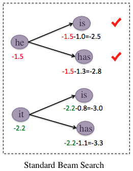
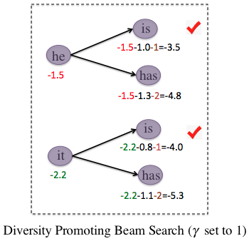
Figure 3.1: An illustration of standard beam search and the proposed diversity-promoting beam search. $\gamma$ denotes the hyperparameter for penalizing intra-sibling ranking. Scores are made up for illustration purposes.

Diversity-Promoting Beam Seach

We propose to increase diversity by changing the way $S(Y_{t-1}^{k},y_{t}^{k,k^{\prime}}|x)$ is computed, as shown in Figure 3.1. For each of the hypotheses $Y_{t-1}^{k}$ (he and it), we generate the top $K$ translations $y_{t}^{k,k^{\prime}}$, $k^{\prime}\in[1,K]$ as in the standard beam search model. Next, we rank the $K$ translated tokens generated from the same parental hypothesis based on $p(y_{t}^{k,k^{\prime}}|x,Y_{t-1}^{k})$ in descending order: he is ranks first among he is and he has, and he has ranks second; similarly for it is and it has.

We then rewrite the score for $[Y_{t-1}^{k},y_{t}^{k,k^{\prime}}]$ by adding an additional term $\gamma k^{\prime}$, where $k^{\prime}$ denotes the ranking of the current hypothesis among its siblings (1 for he is and it is, 2 for he has and it has).

$$\hat{S}(Y_{t-1}^{k},y_{t}^{k,k^{\prime}}|x)=S(Y_{t-1}^{k},y_{t}^{k,k^{\prime}}|x)-\gamma k^{\prime}$$ (3.10)

We call $\gamma$ the diversity rate; it indicates the degree of diversity one wants to integrate into the beam search model.

The top $K$ hypotheses are selected based on $\hat{S}(Y_{t-1}^{k},y_{t}^{k,k^{\prime}}|x)$ as we move on to the next time step. By adding the additional term $\gamma k^{\prime}$, the model punishes lower-ranked hypotheses among siblings (hypotheses descended from the same parent). When we compare newly generated hypotheses descended from different ancestors, the model gives more credit to top hypotheses from each of the different ancestors. For instance, even though the original score for it is is lower than he has, the model favors the former as the latter is more severely punished by the intra-sibling ranking part $\gamma k^{\prime}$. The model thus generally favors choosing hypotheses from diverse parents, leading to a more diverse N-best list. The proposed model is straightforwardly implemented with a minor adjustment to the standard beam search.

3.1.3 Training

Recent research has shown that deep LSTMs work better than single-layer LSTMs for Seq2Seq tasks Sutskever et al. (2014). We adopt a deep structure with four LSTM layers for encoding and four LSTM layers for decoding, each of which consists of a different set of parameters. Each LSTM layer consists of 1,000 hidden neurons, and the dimensionality of word embeddings is set to 1,000. Other training details are given below, broadly aligned with Sutskever et al. (2014).

• LSTM parameters and embeddings are initialized from a uniform distribution in [-0.08, 0.08].

• Stochastic gradient decent is implemented using a fixed learning rate of 0.1.

• Batch size is set to 256.

• Gradient clipping is adopted by scaling gradients when the norm exceeded a threshold of 1.

Our implementation on a single GPU processes at a speed of approximately 600-1200 tokens per second.

The $p(y|x)$ model described in Section 4.3.1 was trained using the same model as that of $p(y|x)$, with messages ($x$) and responses ($y$) interchanged.

3.1.4 Decoding

MMI-antiLM

As described in Section 4.3.1, decoding using $\log p(y|x)-\lambda U(y)$ can be readily implemented by predicting tokens at each time-step. In addition, we found in our experiments that it is also important to take into account the length of responses in decoding. We thus linearly combine the loss function with length penalization, leading to an ultimate score for a given target $T$ as follows:

$$Score(T)=p(y|x)-\lambda U(y)+\gamma L_{y}$$ (3.11)

where $L_{T}$ denotes the length of the target and $\gamma$ denotes associated weight. We optimize $\gamma$ and $\lambda$ using MERT Och (2003) on N-best lists of response candidates. The N-best lists are generated using the decoder with beam size 200. We set a maximum length of 20 for generated candidates. At each time step of decoding, we are presented with $N\times N$ word candidates. We first add all hypotheses with an EOS token being generated at current time step to the N-best list. Next we preserve the top N unfinished hypotheses and move to next time step. We therefore maintain batch size of 200 constant when some hypotheses are completed and taken down by adding in more unfinished hypotheses. This will lead the size of final N-best list for each input much larger than the beam size.

MMI-bidi

We generate N-best lists based on $P(T|S)$ and then rerank the list by linearly combining $p(T|S)$, $\lambda p(S|T)$, and $\gamma L_{T}$. We use MERT Och (2003) to tune the weights $\lambda$ and $\gamma$ on the development set.

Model	$\#$ of training instances	Bleu	distinct-1	distinct-2
Seq2Seq (baseline)	23M	4.31	.023	.107
Seq2Seq (greedy)	23M	4.51	.032	.148
MMI-antiLM: $\log p(y|x)-\lambda U(y)$	23M	4.86	.033	.175
MMI-bidi: $(1-\lambda)\log p(y|s)+\lambda\log p(x|y)$	23M	5.22	.051	.270
SMT Ritter et al. (2011)	50M	3.60	.098	.351
SMT+neural reranking Sordoni et al. (2016)	50M	4.44	.101	.358

Table 3.2: Performance on the Twitter dataset of 4-layer Seq2Seq models and MMI models. distinct-1 and distinct-2 are respectively the number of distinct unigrams and bigrams divided by total number of generated words.

3.2 Experiments

3.2.1 Datasets

Twitter Conversation Triple Dataset

We used an extension of the dataset described in Sordoni et al. (2016), which consists of 23 million conversational snippets randomly selected from a collection of 129M context-message-response triples extracted from the Twitter Firehose over the 3-month period from June through August 2012. For the purposes of our experiments, we limited context to the turn in the conversation immediately preceding the message. In our LSTM models, we used a simple input model in which contexts and messages are concatenated to form the source input.

For tuning and evaluation, we used the development dataset (2118 conversations) and the test dataset (2114 examples), augmented using information retrieval methods to create a multi-reference set. The selection criteria for these two datasets included a component of relevance/interestingness, with the result that dull responses will tend to be penalized in evaluation.

OpenSubtitles Dataset

In addition to unscripted Twitter conversations, we also used the OpenSubtitles (OSDb) dataset Tiedemann (2009), a large, noisy, open-domain dataset containing roughly 60M-70M scripted lines spoken by movie characters. This dataset does not specify which character speaks each subtitle line, which prevents us from inferring speaker turns. Following Vinyals et al. (2015), we make the simplifying assumption that each line of subtitle constitutes a full speaker turn. Our models are trained to predict the current turn given the preceding ones based on the assumption that consecutive turns belong to the same conversation. This introduces a degree of noise, since consecutive lines may not appear in the same conversation or scene, and may not even be spoken by the same character.

This limitation potentially renders the OSDb dataset unreliable for evaluation purposes. For evaluation purposes, we therefore used data from the Internet Movie Script Database (IMSDB), which explicitly identifies which character speaks each line of the script. This allowed us to identify consecutive message-response pairs spoken by different characters. We randomly selected two subsets as development and test datasets, each containing 2K pairs, with source and target length restricted to the range of [6,18].

Model	Bleu	distinct-1	distinct-2
Seq2Seq	7.16	0.0420	0.133
MMI-antiLM	7.60	0.0674	0.220
MMI-bidi	8.26	0.0758	0.288

Table 3.3: Performance on the OpenSubtitles dataset for the Seq2Seq baseline and two MMI models.

3.2.2 Evaluation

For parameter tuning and final evaluation, we used Bleu Papineni et al. (2002), which was shown to correlate reasonably well with human judgment on the response generation task Galley et al. (2015). In the case of the Twitter models, we used multi-reference Bleu. As the IMSDB data is too limited to support extraction of multiple references, only single reference Bleu was used in training and evaluating the OSDb models.

We did not follow Vinyals and Le (2015) in using perplexity as evaluation metric. Perplexity is unlikely to be a useful metric in our scenario, since our proposed model is designed to steer away from the standard Seq2Seq model in order to diversify the outputs. We report degree of diversity by calculating the number of distinct unigrams and bigrams in generated responses. The value is scaled by total number of generated tokens to avoid favoring long sentences (shown as distinct-1 and distinct-2 in Tables 3.2 and 3.3).

3.2.3 Results

Twitter Dataset

We first report performance on Twitter datasets in Table 3.2, along with results for different models (i.e., Machine Translation and MT+neural reranking) reprinted from Sordoni et al. (2016) on the same dataset. The baseline is the Seq2Seq model with its standard likelihood objective and a beam size of 200. We compare this baseline against greedy-search Seq2Seq Vinyals and Le (2015), which achieves higher diversity by increasing search errors.

Machine Translation is the phrase-based MT system described in Ritter et al. (2011). MT features include forward and backward maximum likelihood “translation” probabilities, word and phrase penalties, linear distortion, etc. MT+neural reranking is the phrase-based MT system, reranked using neural models. N-best lists are first generated from the MT system. Recurrent neural models generate scores for N-best list candidates given the input messages. These generated scores are re-incorporated to rerank all the candidates. Additional features to score [1-4]-gram matches between context and response and between message and context (context and message match CMM features) are also employed, as in Sordoni et al. Sordoni et al. (2016).

MT+neural reranking achieves a Bleu score of 4.44, which to the best of our knowledge represents the previous state-of-the-art performance on this Twitter dataset. Note that Machine Translation and MT+neural reranking are trained on a much larger dataset of roughly 50 million examples. A significant performance boost is observed from MMI-bidi over baseline Seq2Seq, both in terms of Bleu score and diversity.

OpenSubtitles Dataset

All models achieve significantly higher Bleu scores on this dataset than on the Twitter dataset, even though the IMSDB data provides only single references for evaluation. Table 3.3 shows that the MMI-bidi model yields a significant performance boost, with a Bleu score increase of up to $15.3\%$ and a more than $116\%$ jump in unigram diversity. Our interpretation of this huge performance improvement is that the diversity and complexity of input messages lead standard Seq2Seq models to generate very conservative responses, which fail to match more the interesting reference strings typical of this dataset.

message	Seq2Seq	MMI $P(T|S)-\lambda P(T)$
I did not get the report from an mi-6 agent.	I don’t think that’s a good idea.	You did the right thing, did you?
You haven’t been given an assignment in this case.	I don’t know what you are talking about.	I’ve been looking all over for you.
I’m losing my grip.	I don’t know what you are talking about.	I’m the only one in the world.
I am ready to help.	Come on, come on	I have something we need to talk about.
You programmed me to gather intelligence. That’s all I’ve ever done.	You know that, don’t you?	You do have fun, don’t you?
I mean, we’d have to talk to him.	I mean, I don’t know.	I mean, he’s a good guy.
This has nothing to do with him.	You don’t know anything about him, do you?	I know him as much.
How come you never say it?	I don’t know	Because I don’t want to hurt you
He is the one behind this scheme to crash x-net.	I don’t know what you are talking about	Yes, he is, isn’t he?
How much time do you have here?	I don’t know.	Not long enough. Sorry, sir.

Table 3.4: Responses from the Seq2Seq baseline and MMI-antiLM models on the OpenSubtitles dataset.

message	Seq2Seq	MMI-bidi
Ohh I’ve never seen that! How long does it take you guys to learn the drill?	I don’t even know.	Like 2 weeks ago!!
You’ll know when we sign Heskey in 2 weeks	I’ll see what I can do	I sure hope so..
I’m waiting!! I have even got biscuits waiting for you??	I have no idea what you’re talking about	I’ll send you a pic when I get home xx
My parents actually had touch too much played at their wedding.	I have no idea what you’re talking about	How old are they??
Say anything you want… I know you love me and I love you.	I love you so much.	I love you too, baby.
I am off all week next week	What time you going?	What time you going?
How are you doing?	I’m good, thanks.	I’m good, you?

Table 3.5: Responses from the Seq2Seq baseline and MMI-bidi models on the Twitter dataset.

Comparator	Gain	95% CI
SMT Ritter et al. (2011)	0.29	[0.25, 0.32]
SMT+neural reranking	0.28	[0.25, 0.32]
Seq2Seq (baseline)	0.11	[0.07, 0.14]
Seq2Seq (greedy)	0.08	[0.04, 0.11]

Table 3.6: MMI-bidi gains over comparator systems, based on pairwise human judgments.

Input: What are you doing?
1. I’ve been looking for you.	4. I told you to shut up.
2. I want to talk to you.	5. Get out of here.
3. Just making sure you’re OK.	6. I’m looking for a doctor.
Input: What is your name?
1. Blue!	4. Daniel.
2. Peter.	5. My name is John.
3. Tyler.	6. My name is Robert.
Input: How old are you?
1. Twenty-eight.	4. Five.
2. Twenty-four.	5. 15.
3. Long.	6. Eight.

Table 3.7: Examples generated by the MMI-antiLM model on the OpenSubtitles dataset.

Qualitative Evaluation

We employed crowdsourced judges to provide evaluations for a random sample of 1000 items in the Twitter test dataset. Table 3.6 shows the results of human evaluations between paired systems. Each output pair was ranked by 5 judges, who were asked to decide which of the two outputs was better. They were instructed to prefer outputs that were more specific (relevant) to the message and preceding context, as opposed to those that were more generic. Ties were permitted. Identical strings were algorithmically assigned the same score. The mean of differences between outputs is shown as the gain for MMI-bidi over the competing system. At a significance level of $\alpha=0.05$, we find that MMI-bidi outperforms both baseline and greedy Seq2Seq systems, as well as the weaker SMT and SMT+RNN baselines. MMI-bidi outperforms SMT in human evaluations despite the greater lexical diversity of MT output.

Separately, judges were also asked to rate overall quality of MMI-bidi output over the same 1000-item sample in isolation, each output being evaluated by 7 judges in context using a 5-point scale. The mean rating was 3.84 (median: 3.85, 1st Qu: 3.57, 3rd Qu: 4.14), suggesting that overall MMI-bidi output does appear reasonably acceptable to human judges.

Table 3.7 presents the N-best candidates generated using the MMI-bidi model for the inputs of Table 3.1. We see that MMI generates significantly more interesting outputs than Seq2Seq.

In Tables 3.4 and 3.5, we present responses generated by different models. All examples were randomly sampled (without cherry picking). We see that the baseline Seq2Seq model tends to generate reasonable responses to simple messages such as How are you doing? or I love you. As the complexity of the message increases, however, the outputs switch to more conservative, duller forms, such as I don’t know or I don’t know what you are talking about. An occasional answer of this kind might go unnoticed in a natural conversation, but a dialog agent that always produces such responses risks being perceived as uncooperative. MMI-bidi models, on the other hand, produce far more diverse and interesting responses.

3.3 Conclusions

In this chapter, we investigated the issue that Seq2Seq models tend to generate safe, commonplace responses (e.g., I don’t know) regardless of the input. Our analysis suggests that the issue is at least in part attributable to the use of unidirectional likelihood of output (responses) given input (messages). To remedy this, we have proposed using Maximum Mutual Information (MMI) as the objective function. Our results demonstrate that the proposed MMI models produce more diverse and interesting responses, while improving quality as measured by Bleu and human evaluation.

Chapter 4 Addressing the Speaker Consistency Issue

One severe issue for current chit-chat systems is their lack of speaker consistency. Since the training set contains conversations from different people, and a decoding model always selects the response with the greatest likelihood, outputs can be wildly inconsistent, as illustrated in Table 4.1.

m:	Where do you live now?	m:	Where were you born?
r:	I live in Los Angeles.	r:	I was born in Canada.
m:	In which city do you live now?	m:	Where are you from?
r:	I live in Madrid.	r:	England, you?
m:	In which country do you live now?	m:	Where did you grow up?
r:	England, you?	r:	I grew up in Texas.
m:	How old are you?	m:	What is your major?
r:	16 and you?	r:	I’m majoring in psychology
m:	What’s your age?	m:	What did you study in college?
r:	16.	r:	I studied psychology.

Table 4.1: Inconsistent responses generated by a 4-layer Seq2Seq model trained on 25 million Twitter conversation snippets. m denotes input message and r denotes the generated response.

In this chapter, we talk about how we can address the challenge of consistency and how to endow data-driven systems with the coherent “persona” needed to model human-like behavior, whether as personal assistants, personalized avatar-like agents, or game characters. For present purposes, we will define persona as the character that an artificial agent, as actor, plays or performs during conversational interactions. A persona can be viewed as a composite of elements of identity (background facts or user profile), language behavior, and interaction style. A persona is also adaptive, since an agent may need to present different facets to different human interlocutors depending on the demands of the interaction.

We explore two persona models, a single-speaker Speaker Model and a dyadic Speaker-Addressee Model, within the Seq2Seq framework. The Speaker Model integrates a speaker-level vector representation into the target part of the Seq2Seq model. Analogously, the Speaker-Addressee model encodes the interaction patterns of two interlocutors by constructing an interaction representation from their individual embeddings and incorporating it into the Seq2Seq model. These persona vectors are trained on human-human conversation data and used at test time to generate personalized responses. Our experiments on an open-domain corpus of Twitter conversations and dialog datasets comprising TV series scripts show that leveraging persona vectors can improve relative performance up to $20\%$ in Bleu score and $12\%$ in perplexity, with a commensurate gain in consistency as judged by human annotators.

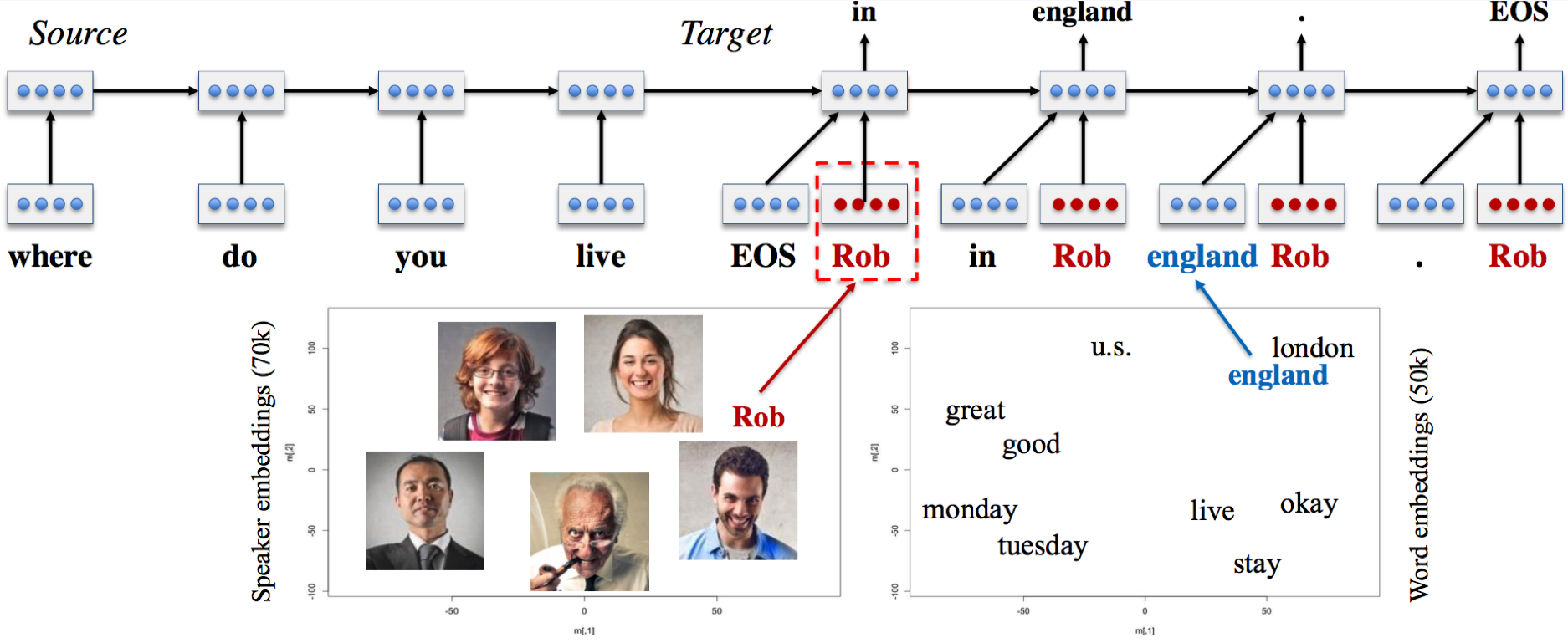
Figure 4.1: Illustrative example of the Speaker Model introduced in this work. Speaker IDs close in embedding space tend to respond in the same manner. These speaker embeddins are learned jointly with word embeddings and all other parameters of the neural model via backpropagation. In this example, say Rob is a speaker clustered with people who often mention England in the training data, then the generation of the token ‘england’ at time $t=2$ would be much more likely than that of ‘u.s.’. A non-persona model would prefer generating in the u.s. if ‘u.s.’ is more represented in the training data across all speakers.

4.1 Model

4.1.1 Speaker Model

Our first model is the Speaker Model, which models the respondent alone. This model represents each individual speaker as a vector or embedding, which encodes speaker-specific information (e.g., dialect, register, age, gender, personal information) that influences the content and style of her responses.

Figure 4.1 gives a brief illustration of the Speaker Model. Each speaker $i\in[1,N]$ is associated with a user-level representation $v_{i}\in\mathbb{R}^{K\times 1}$. As in standard Seq2Seq models, we first encode message $S$ into a vector representation $h_{S}$ using the source LSTM. Then for each step in the target side, hidden units are obtained by combining the representation produced by the target LSTM at the previous time step (i.e., $h_{t-1}$), the word representations at the current time step $x_{t}$, and the speaker embedding $v_{i}$:

$$\left[\begin{array}[]{lr}i_{t}\\ f_{t}\\ o_{t}\\ l_{t}\\ \end{array}\right]=\left[\begin{array}[]{c}\sigma\\ \sigma\\ \sigma\\ \tanh\\ \end{array}\right]W\cdot\left[\begin{array}[]{c}v_{i}\\ h_{t-1}\\ x_{t}\\ \end{array}\right]$$ (4.1)

$$c_{t}=f_{t}\cdot c_{t-1}+i_{t}\cdot l_{t}$$ (4.2)

$$h_{t}=o_{t}\cdot\tanh(c_{t})$$ (4.3)

where $W\in\mathbb{R}^{4K\times 3K}$. In this way, speaker information is encoded and injected into the hidden layer at each time step and thus helps predict personalized responses throughout the generation process. The Speaker embedding $\{v_{i}\}$ is shared across all conversations that involve speaker $i$. $\{v_{i}\}$ are learned by back propagating word prediction errors to each neural component during training.

Another helpful property of this model is that it helps infer answers to questions even if the evidence is not readily present in the training set. This is important as the training data does not contain explicit information about every attribute of each user (e.g., gender, age, country of residence).

The model learns speaker representations based on conversational content produced by different speakers, and speakers producing similar responses tend to have similar embeddings, occupying nearby positions in the vector space. This way, the training data of speakers nearby in vector space help increase the generalization capability of the speaker model. For example, consider two speakers $i$ and $j$ who sound distinctly British, and who are therefore close in speaker embedding space. Now, suppose that, in the training data, speaker $i$ was asked Where do you live? and responded in the UK. Even if speaker $j$ was never asked the same question, this answer can help influence a good response from speaker $j$, and this without any explicitly labeled geo-location information.

4.1.2 Speaker-Addressee Model

A natural extension of the Speaker Model is a model that is sensitive to speaker-addressee interaction patterns within the conversation. Indeed, speaking style, register, and content does not only vary with the identity of the speaker, but also with that of the addressee. For example, in scripts for the TV series Friends used in some of our experiments, the character Ross often talks differently to his sister Monica than to Rachel, with whom he is engaged in a on-again off-again relationship throughout the series.

The proposed Speaker-Addressee Model operates as follows: We wish to predict how speaker $i$ would respond to a message produced by speaker $j$. Similarly to the Speaker model, we associate each speaker with a $K$ dimensional speaker-level representation, namely $v_{i}$ for user $i$ and $v_{j}$ for user $j$. We obtain an interactive representation $V_{i,j}\in\mathbb{R}^{K\times 1}$ by linearly combining user vectors $v_{i}$ and $v_{j}$ in an attempt to model the interactive style of user $i$ towards user $j$,

$$V_{i,j}=\tanh(W_{1}\cdot v_{i}+W_{2}\cdot v_{2})$$ (4.4)

where $W_{1},W_{2}\in\mathbb{R}^{K\times K}$. $V_{i,j}$ is then linearly incorporated into LSTM models at each step in the target:

$$\left[\begin{array}[]{lr}i_{t}\\ f_{t}\\ o_{t}\\ l_{t}\\ \end{array}\right]=\left[\begin{array}[]{c}\sigma\\ \sigma\\ \sigma\\ \tanh\\ \end{array}\right]W\cdot\left[\begin{array}[]{c}h_{t-1}\\ w_{t}\\ V_{i,j}\\ \end{array}\right]$$ (4.5)

$$c_{t}=f_{t}\cdot c_{t-1}+i_{t}\cdot l_{t}\\$$ (4.6)

$$h_{t}=o_{t}\cdot\tanh(c_{t})$$ (4.7)

$V_{i,j}$ depends on both speaker and addressee and the same speaker will thus respond differently to a message from different interlocutors. One potential issue with Speaker-Addressee modelling is the difficulty involved in collecting a large-scale training dataset in which each speaker is involved in conversation with a wide variety of people. Like the Speaker Model, however, the Speaker-Addressee Model derives generalization capabilities from speaker embeddings. Even if the two speakers at test time ($i$ and $j$) were never involved in the same conversation in the training data, two speakers $i^{\prime}$ and $j^{\prime}$ who are respectively close in embeddings may have been, and this can help modelling how $i$ should respond to $j$.

4.1.3 Decoding and Reranking

For decoding, the N-best lists are generated using the decoder with beam size $K=200$. We set a maximum length of 20 for the generated candidates. To deal with the issue that Seq2Seq models tend to generate generic and commonplace responses such as I don’t know, we follow Li et al. (2016a) by reranking the generated N-best list using a scoring function that linearly combines a length penalty and the log likelihood of source given target:

$$\log p(y|x,v)+\lambda\log p(x|y)+\gamma L_{y}$$ (4.8)

where $p(y|x,v)$ denotes the probability of the generated response given the message $x$ and the respondent’s speaker ID. $L_{y}$ denotes the length of the target and $\gamma$ denotes the associated penalty weight. We optimize $\gamma$ and $\lambda$ on N-best lists of response candidates generated from the development set using MERT Och (2003) by optimizing Bleu. To compute $p(x|y)$, we train an inverse Seq2Seq model by swapping messages and responses. We trained standard Seq2Seq models for $p(x|y)$ with no speaker information considered.

4.2 Experiements

Following Sordoni et al. (2016); Li et al. (2016a) we used Bleu Papineni et al. (2002) for parameter tuning and evaluation. Besides Bleu scores, we also report perplexity, which has been widely adopted as an indicator of model capability.

System	Bleu
MT baseline Ritter et al. (2011)	3.60%
Standard LSTM MMI Li et al. (2016a)	5.26%
Standard LSTM MMI (our system)	5.82%
Human	6.08%

Table 4.2: Bleu on the Twitter Sordoni dataset (10 references). We contrast our baseline against an SMT baseline Ritter et al. (2011), and the best result Li et al. (2016a) on the established dataset of Sordoni et al. (2016). The last result is for a human oracle, but it is not directly comparable as the oracle Bleu is computed in a leave-one-out fashion, having one less reference available. We nevertheless provide this result to give a sense that these Bleu scores of 5-6% are not unreasonable.

4.2.1 Baseline

Since our main experiments are with a new dataset (the Twitter Persona Dataset), we first show that our LSTM baseline is competitive with the state-of-the-art Li et al. (2016a) on an established dataset, the Twitter Dataset Sordoni et al. (2016). Our baseline is simply our implementation of the LSTM-MMI of Li et al. (2016a), so results should be relatively close to their reported results. Table 4.2 summarizes our results against prior work. We see that our system actually does better than Li et al. (2016a), and we attribute the improvement to a larger training corpus, the use of dropout during training, and possibly to the “conversationalist” nature of our corpus.

Model	Standard LSTM	Speaker Model
Perplexity	47.2	42.2 ($-10.6\%$)

Table 4.3: Perplexity for standard Seq2Seq and the Speaker model on the development set of the Twitter Persona dataset.

Model	Objective	Bleu
Standard LSTM	MLE	0.92%
Speaker Model	MLE	1.12%
Standard LSTM	MMI	1.41%
Speaker Model	MMI	1.66%

Table 4.4: Bleu on the Twitter Persona dataset (1 reference), for the standard Seq2Seq model and the Speaker model using as objective either maximum likelihood (MLE) or maximum mutual information (MMI).

Model	Standard LSTM	Speaker Model	Speaker-Addressee Model
Perplexity	27.3	25.4 ($-7.0\%$)	25.0 ($-8.4\%$)

Table 4.5: Perplexity for standard Seq2Seq and persona models on the TV series dataset.

Model	Standard LSTM	Speaker Model	Speaker-Addressee Model
MLE	1.60%	1.82% ($+13.7\%$)	1.83% ($+14.3\%$)
MMI	1.70%	1.90% ($+10.6\%$)	1.88% ($+10.9\%$)

Table 4.6: Bleu on the TV series dataset (1 reference), for the standard Seq2Seq and persona models.

4.2.2 Results

We first report performance on the Twitter Persona dataset. Perplexity is reported in Table 4.3. We observe about a $10\%$ decrease in perplexity for the Speaker model over the standard Seq2Seq model. In terms of Bleu scores (Table 4.4), a significant performance boost is observed for the Speaker model over the standard Seq2Seq model, yielding an increase of $21\%$ in the maximum likelihood (MLE) setting and $11.7\%$ for mutual information setting (MMI). In line with findings in Li et al. (2016a), we observe a consistent performance boost introduced by the MMI objective function over a standard Seq2Seq model based on the MLE objective function. It is worth noting that our persona models are more beneficial to the MLE models than to the MMI models. This result is intuitive as the persona models help make Standard LSTM MLE outputs more informative and less bland, and thus make the use of MMI less critical.

For the TV Series dataset, perplexity and Bleu scores are respectively reported in Table 4.5 and Table 4.6. As can be seen, the Speaker and Speaker-Addressee models respectively achieve perplexity values of 25.4 and 25.0 on the TV-series dataset, $7.0\%$ and $8.4\%$ percent lower than the correspondent standard Seq2Seq models. In terms of Bleu score, we observe a similar performance boost as on the Twitter dataset, in which the Speaker model and the Speaker-Addressee model outperform the standard Seq2Seq model by $13.7\%$ and $10.6\%$. By comparing the Speaker-Addressee model against the Speaker model on the TV Series dataset, we do not observe a significant difference. We suspect that this is primarily due to the relatively small size of the dataset where the interactive patterns might not be fully captured. Smaller values of perplexity are observed for the Television Series dataset than the Twitter dataset, the perplexity of which is over 40, presumably due to the more noisy nature of Twitter dialogues.

4.2.3 Qualitative Analysis

message	Where is your hometown?	message	What company do you work for?
baseline	I was born in Canada.	baseline	I work for a company.
user1	I’m from England.	user1	I don’t have a job.
user2	I’m from Manchester.	user2	I’m a manager.
user3	I’m from Liverpool.	user3	I’m working. $\#$
user4	England. You?	user4	I work for a company
user5	My hometown.	user5	I’m working. $\#$
user6	I’m from Texas.	user6	Customer service.
user7	I’m from LA.	user7	I work in retail.
user8	England.	user8	I work in a cafe.
user9	I was born here.	user9	I work at a gas station.
user10	I was born in the us.	user10	I don’t know $\#$

Table 4.7: Responses generated by the baseline (LSTM-MMI) and the Speaker Model for ten randomly selected users, without cherry picking. $\#$ indicates poor-quality responses produced by the system.

message	Do you love me ?
baseline	of course, i love you .
	addressee Emily, speaker Sheldon
response	of course, i love you, emily .
	addressee Emily, speaker Penny
response	of course, i love you, emily .
	addressee Lenard, speaker Penny
response	of course, i love you, Lenard .
	addressee Monica, speaker Chandler
response	of course i love you . i want to marry you .
	addressee Rachel, speaker Chandler
response	of course i love you .
	addressee Ross, speaker Chandler
response	of course i love you .
	addressee Ross, speaker Rachel
response	of course i love you . ( kisses him )
	addressee Emily, speaker Rachel
response	of course i love you .

Table 4.8: Responses to do you love me from the addressee-speaker model on the TV-series dataset using different addressees and speakers.

Diverse Responses by Different Speakers

Table 4.7 represents responses generated by persona models in response to three different input questions. We randomly selected 10 speakers (without cherry-picking) from the original Twitter dataset. We collected their user level representations from a speaker look-up table and integrated them into the decoding models. We can see that the model tends to generate specific responses for different people in response to the factual questions.

Table 4.8 represents responses generated from the Speaker-Addressee Model using the TV-series dataset. Interestingly, we do observe the subtle difference captured by the model when it attempts to respond to different addresses . For example, the model produces of course, i love you, emily . in response to input from addresseeEmily by generating the addressee’s name. Also, the model generates of course i love you . ( kisses him ) in response to female addressees.

Human Evaluation

We conducted a human evaluation of outputs from the Speaker Model, using a crowdsourcing service. Since we cannot expect crowdsourced human judges to know or attempt to learn the ground truth of Twitter users who are not well-known public figures, we designed our experiment to evaluate the consistency of outputs associated with the speaker IDs. To this end, we collected 24 pairs of questions for which we would expect responses to be consistent if the persona model is coherent. For example, responses to the questions What country do you live in? and What city do you live in? would be considered consistent if the answers were England and London respectively, but not if they were UK and Chicago. Similarly, the responses to Are you vegan or vegetarian? and Do you eat beef? are consistent if the answers generated are vegan and absolutely not, but not if they are vegan and I love beef. We collected the top 20 pairs of outputs provided by the Speaker Model for each question pair (480 response pairs total). We also obtained the corresponding outputs from the baseline MMI-enhanced Seq2Seq system.

Since our purpose is to measure the gain in consistency over the baseline system, we presented the pairs of answers system-pairwise, i.e., 4 responses, 2 from each system, displayed on the screen. Then we asked judges to decide which of the two systems was more consistent. The position in which the system pairs were presented on the screen was randomized. Five judges rated each pair. A system was assigned a score 1.0 if it was judged much more consistent than the other, 0.5 if mostly more consistent, zero otherwise. Ties (where the two systems are equally consistent or inconsistent) were discarded. A maximum score of 5.0 was possible. After reweighting for frequency of response pairs, the mean relative consistency rating for the Speaker Model was 1.33 compared to 0.99 for the baseline model, representing a gain in relative consistency of 34.68%. It should be stressed that the latter is a strong baseline, since it represents the consensus of all 70K Twitter users in the dataset. (I’m not pregnant is an excellent consensus answer to the question Are you pregnant?, while I’m pregnant is consistent as a response only in the case of someone who also answers the question Are you a guy or a girl? with something in the vein of I’m a girl.)

Speaker Consistency

Table 4.9 illustrates how consistency is an emergent property of two arbitrarily selected users. The model is capable of discovering the relations between different categories of location such as London and the UK, Jakarta and Indonesia. However, the model also makes inconsistent response decisions, generating different answers in the second example in response to questions asking about age or major. Our proposed persona models integrate user embeddings into the LSTM, and thus can be viewed as encapsulating a trade-off between a persona-specific generation model and a general conversational model.

User1		User2
message	Where is your hometown?	message	Where is your hometown?
response	I’m from England.	response	I live in Indonesia.
message	Where are you from?	message	Where are you from?
response	I’m from England.	response	England, you?
message	In which city do you live now?	message	In which city do you live now?
response	I live in London.	response	I live in Jakarta.
message	In which country do you live now?	message	In which country do you live now?
response	I live in England.	response	I live in Indonesia.
message	What is your major?	message	What is your major?
response	Business. You?	response	Business, you?
message	What did you study in college?	message	What did you study in college?
response	I did business studies.	response	Psychology, you?
message	How old are you?	message	How old are you?
response	I’m 18.	response	I’m 18.
message	What is your age?	response	What is your age?
response	I’m 18.	response	I’m 16.

Table 4.9: Examples of speaker consistency and inconsistency generated by the Speaker Model

4.3 Conclusion

In this chapter, we have presented two persona-based response generation models for open-domain conversation generation.

Although the gains presented by our new models are not spectacular, the systems nevertheless outperform our baseline Seq2Seq systems in terms of Bleu, perplexity, and human judgments of speaker consistency. We have demonstrated that by encoding personas into distributed representations, we are able to capture certain personal characteristics such as speaking style and background information. In the Speaker-Addressee model, moreover, the evidence suggests that there is benefit in capturing dyadic interactions.

Our ultimate goal is to be able to take the profile of an arbitrary individual whose identity is not known in advance, and generate conversations that accurately emulate that individual’s persona in terms of linguistic response behavior and other salient characteristics. Such a capability will dramatically change the ways in which we interact with dialog agents of all kinds, opening up rich new possibilities for user interfaces. Given a sufficiently large training corpus in which a sufficiently rich variety of speakers is represented, this objective does not seem too far-fetched.

Chapter 5 Fostering Long-term Dialogue Success

In the previous two sections, we have talked about how a chit-chat system can avoid general responses and produce consistent responses regarding different questions. So far, we have only been concerned with the quality of single-turn responses, but this is actually an overly simplified approximation of humans’ conversations. Humans’ conversations usually consist of tens, or even hundreds of turns. These multi-turn conversations usually have structures, e.g., starting with an opener, setting up contexts, getting to the points, etc, and humans are good at managing the informational flow of a conversation, that lead to the long-term success (including overall coherence, meaningfulness, etc) of a conversation.

Current models are trained by predicting the next dialogue turn in a given conversational context using the maximum-likelihood estimation (MLE) objective function. Its incapability of handling this conversational long-term success results in many pitfalls: First, the fact that Seq2Seq models tend to generate highly generic responses, as discussed in Chapter 3 actually results from this incapability: responses such as “I don’t know” are apparently not a good action to take in long term, since it closes the conversation down; Second, as illustrated in the two sample conversations on the left of Table 5.1, the system becomes stuck in an infinite loop of repetitive responses. This is due to MLE-based Seq2Seq models’ inability to account for repetition. In example 2 (bottom left), the dialogue falls into an infinite loop after three turns, with both agents generating dull, generic utterances like i don’t know what you are talking about and you don’t know what you are saying. Looking at the entire conversation, utterance (4) turns out to be a bad action to take because it offers no way of continuing the conversation.

Baseline mutual information model	Proposed reinforcement learning model
A: Where are you going? (1)	A: Where are you going? (1)
B: I’m going to the restroom. (2)	B: I’m going to the police station. (2)
A: See you later. (3)	A: I’ll come with you. (3)
B: See you later. (4)	B: No, no, no, no, you’re not going anywhere. (4)
A: See you later. (5)	A: Why? (5)
B: See you later. (6)	B: I need you to stay here. (6)
…	A: I don’t know what you are talking about. (7)
…	…
A: how old are you? (1)	A: How old are you? (1)
B: I’m 16. (2)	B: I’m 16. Why are you asking? (2)
A: 16? (3)	A I thought you were 12. (3)
B: I don’t know what you are talking about. (4)	B: What made you think so? (4)
A: You don’t know what you are saying. (5)	A: I don’t know what you are talking about. (5)
B: I don’t know what you are talking about . (6)	B: You don’t know what you are saying. (6)
A: You don’t know what you are saying. (7)	…
…	…

Table 5.1: Left Column: Dialogue simulation between two agents using a Seq2Seq trained on the OpenSubtitles dataset. The first turn (index 1) is input by the authors. Then the two agents take turns conversing, taking as input the other agent’s prior generated turn. The output is generated using the mutual information model Li et al. (2016a) in which an N-best list is first obtained using beam search based on p(t$|$s) and reranked by linearly combining the backward probability p(s$|$t), where t and s respectively denote targets and sources. Right Column: Dialogue simulated using the proposed reinforcement learning model. The new model has more forward-looking utterances (questions like “Why are you asking?” and offers like “I’ll come with you”) and lasts longer before it falls into conversational black holes.

These challenges suggest we need a conversation framework that has the ability to (1) integrate developer-defined rewards that better mimic the true goal of chatbot development and (2) model the long-term influence of a generated response in an ongoing dialogue.

To achieve these goals, we draw on the insights of reinforcement learning, which have been widely applied in MDP and POMDP dialogue systems (see Related Work section for details). We introduce a neural reinforcement learning (RL) generation method, which can optimize long-term rewards designed by system developers. Our model uses the encoder-decoder architecture as its backbone, and simulates conversation between two virtual agents to explore the space of possible actions while learning to maximize expected reward. We define simple heuristic approximations to rewards that characterize good conversations: good conversations are forward-looking Allwood et al. (1992) or interactive (a turn suggests a following turn), informative, and coherent. The parameters of an encoder-decoder RNN define a policy over an infinite action space consisting of all possible utterances. The agent learns a policy by optimizing the long-term developer-defined reward from ongoing dialogue simulations using policy gradient methods Williams (1992), rather than the MLE objective defined in standard Seq2Seq models.

Our model thus integrates the power of Seq2Seq systems to learn compositional semantic meanings of utterances with the strengths of reinforcement learning in optimizing for long-term goals across a conversation. Experimental results (sampled results at the right panel of Table 5.1) demonstrate that our approach fosters a more sustained dialogue and manages to produce more interactive responses than standard Seq2Seq models trained using the MLE objective.

5.1 Model

In this section, we describe in detail the components of the proposed RL model. The learning system consists of two agents. We use $p$ to denote sentences generated from the first agent and $q$ to denote sentences from the second. The two agents take turns talking with each other. A dialogue can be represented as an alternating sequence of sentences generated by the two agents: $p_{1},q_{1},p_{2},q_{2},...,p_{i},q_{i}$. We view the generated sentences as actions that are taken according to a policy defined by an encoder-decoder recurrent neural network language model.

The parameters of the network are optimized to maximize the expected future reward using policy search. Policy gradient methods are more appropriate for our scenario than Q-learning Mnih et al. (2013), because we can initialize the encoder-decoder RNN using MLE parameters that already produce plausible responses, before changing the objective and tuning towards a policy that maximizes long-term reward. Q-learning, on the other hand, directly estimates the future expected reward of each action, which can differ from the MLE objective by orders of magnitude, thus making MLE parameters inappropriate for initialization. The components (states, actions, reward, etc.) of our sequential decision problem are summarized in the following sub-sections.

5.1.1 Action

An action $a$ is the dialogue utterance to generate. The action space is infinite since arbitrary-length sequences can be generated.

5.1.2 State

A state is denoted by the previous two dialogue turns $[p_{i},q_{i}]$. The dialogue history is further transformed to a vector representation by feeding the concatenation of $p_{i}$ and $q_{i}$ into an LSTM encoder model as described in Li et al. (2016a).

5.1.3 Policy

A policy takes the form of an LSTM encoder-decoder (i.e., $p_{RL}(p_{i+1}|p_{i},q_{i})$ ) and is defined by its parameters. Note that we use a stochastic representation of the policy (a probability distribution over actions given states). A deterministic policy would result in a discontinuous objective that is difficult to optimize using gradient-based methods.

5.1.4 Reward

$r$ denotes the reward obtained for each action. In this subsection, we discuss major factors that contribute to the success of a dialogue and describe how approximations to these factors can be operationalized in computable reward functions.

Ease of answering

A turn generated by a machine should be easy to respond to. This aspect of a turn is related to its forward-looking function: the constraints a turn places on the next turn Allwood et al. (1992). We propose measuring the ease of answering a generated turn by using the negative log likelihood of responding to that utterance with a dull response. We manually constructed a list of dull responses $\mathbb{S}$ consisting 8 dialogue utterances such as “I don’t know what you are talking about”, “I have no idea”, etc., that we and others have found occur very frequently in Seq2Seq models of conversations. The reward function is given as follows:

$$r_{1}=-\frac{1}{N_{\mathbb{S}}}\sum_{s\in\mathbb{S}}\frac{1}{N_{s}}\log p_{\text{seq2seq}}(s|a)$$ (5.1)

where $N_{\mathbb{S}}$ denotes the number of dull responses that we predefined and $N_{s}$ denotes the number of tokens in the dull response $s$. Although of course there are more ways to generate dull responses than the list can cover, many of these responses are likely to fall into similar regions in the vector space computed by the model. A system less likely to generate utterances in the list is thus also less likely to generate other dull responses.

$p_{\text{seq2seq}}$ represents the likelihood output by Seq2Seq models. It is worth noting that $p_{\text{seq2seq}}$ is different from the stochastic policy function $p_{RL}(p_{i+1}|p_{i},q_{i})$, since the former is learned based on the MLE objective of the Seq2Seq model while the latter is the policy optimized for long-term future reward in the RL setting.

Information Flow

We want each agent to contribute new information at each turn to keep the dialogue moving and avoid repetitive sequences. We therefore propose penalizing semantic similarity between consecutive turns from the same agent. Let $h_{p_{i}}$ and $h_{p_{i+1}}$ denote representations obtained from the encoder for two consecutive turns $p_{i}$ and $p_{i+1}$. The reward is given by the negative log of the cosine similarity between them:

$$r_{2}=-\log\text{cos}(h_{p_{i}},h_{p_{i+1}})=-\log\text{cos}\frac{h_{p_{i}}\cdot h_{p_{i+1}}}{\lVert h_{p_{i}}\rVert\lVert h_{p_{i+1}}\rVert}$$ (5.2)

Semantic Coherence

We also need to measure the adequacy of responses to avoid situations in which the generated replies are highly rewarded but are ungrammatical or not coherent. We therefore consider the mutual information between the action $a$ and previous turns in the history to ensure the generated responses are coherent and appropriate:

$$r_{3}=\frac{1}{N_{a}}\log p_{\text{seq2seq}}(a|q_{i},p_{i})+\frac{1}{N_{q_{i}}}\log p_{\text{seq2seq}}^{\text{backward}}(q_{i}|a)$$ (5.3)

$p_{\text{seq2seq}}(a|p_{i},q_{i})$ denotes the probability of generating response $a$ given the previous dialogue utterances $[p_{i},q_{i}]$. $p_{\text{seq2seq}}^{\text{backward}}(q_{i}|a)$ denotes the backward probability of generating the previous dialogue utterance $q_{i}$ based on response $a$. $p_{\text{seq2seq}}^{\text{backward}}$ is trained in a similar way as standard Seq2Seq models with sources and targets swapped. Again, to control the influence of target length, both $\log p_{\text{seq2seq}}(a|q_{i},p_{i})$ and $\log p_{\text{seq2seq}}^{\text{backward}}(q_{i}|a)$ are scaled by the length of targets. The final reward for action $a$ is a weighted sum of the rewards discussed above:

$$r(a,[p_{i},q_{i}])=\lambda_{1}r_{1}+\lambda_{2}r_{2}+\lambda_{3}r_{3}$$ (5.4)

The central idea behind our approach is to simulate the process of two virtual agents taking turns talking with each other, through which we can explore the state-action space and learn a policy $p_{RL}(p_{i+1}|p_{i},q_{i})$ that leads to the optimal expected reward. We adopt an AlphaGo-style strategy Silver et al. (2016) by initializing the RL system using a general response generation policy which is learned from a fully supervised setting.

5.2 Simulation

5.2.1 Supervised Learning

For the first stage of training, we build on prior work of predicting a generated target sequence given dialogue history using the supervised Seq2Seq model Vinyals and Le (2015). Results from supervised models will be later used for initialization.

We trained a Seq2Seq model with attention Bahdanau et al. (2014) on the OpenSubtitles dataset, which consists of roughly 80 million source-target pairs. We treated each turn in the dataset as a target and the concatenation of two previous sentences as source inputs.

5.2.2 Mutual Information

Samples from Seq2Seq models are often times dull and generic, e.g., “i don’t know” Li et al. (2016a). We thus do not want to initialize the policy model using the pre-trained Seq2Seq models because this will lead to a lack of diversity in the RL models’ experiences. Li et al. (2016a) showed that modeling mutual information between sources and targets will significantly decrease the chance of generating dull responses and improve general response quality. We now show how we can obtain an encoder-decoder model which generates maximum mutual information responses.

As illustrated in Li et al. (2016a), direct decoding from Eq 5.3 is infeasible since the second term requires the target sentence to be completely generated. Inspired by recent work on sequence level learning Ranzato et al. (2015), we treat the problem of generating maximum mutual information response as a reinforcement learning problem in which a reward of mutual information value is observed when the model arrives at the end of a sequence.

Similar to Ranzato et al. (2015), we use policy gradient methods Sutton (1999); Williams (1992) for optimization. We initialize the policy model $p_{RL}$ using a pre-trained $p_{{{\textsc{Seq2Seq}}}}(a|p_{i},q_{i})$ model. Given an input source $[p_{i},q_{i}]$, we generate a candidate list $A=\{\hat{a}|\hat{a}\sim p_{RL}\}$. For each generated candidate $\hat{a}$, we will obtain the mutual information score $m(\hat{a},[p_{i},q_{i}])$ from the pre-trained $p_{{{\textsc{Seq2Seq}}}}(a|p_{i},q_{i})$ and $p^{\text{backward}}_{{{\textsc{Seq2Seq}}}}(q_{i}|a)$. This mutual information score will be used as a reward and back-propagated to the encoder-decoder model, tailoring it to generate sequences with higher rewards. We refer the readers to Zaremba and Sutskever (2015) and Williams (1992) for details. The expected reward for a sequence is given by:

$$J(\theta)=\mathbb{E}[m(\hat{a},[p_{i},q_{i}])]$$ (5.5)

The gradient is estimated using the likelihood ratio trick:

$$\nabla J(\theta)=m(\hat{a},[p_{i},q_{i}])\nabla\log p_{RL}(\hat{a}|[p_{i},q_{i}])$$ (5.6)

We update the parameters in the encoder-decoder model using stochastic gradient descent. A curriculum learning strategy is adopted Bengio et al. (2009) as in Ranzato et al. (2015) such that, for every sequence of length $T$ we use the MLE loss for the first $L$ tokens and the reinforcement algorithm for the remaining $T-L$ tokens. We gradually anneal the value of $L$ to zero. A baseline strategy is employed to decrease the learning variance: an additional neural model takes as inputs the generated target and the initial source and outputs a baseline value, similar to the strategy adopted by Zaremba and Sutskever (2015). The final gradient is thus:

$$\nabla J(\theta)=\nabla\log p_{RL}(\hat{a}|[p_{i},q_{i}])[m(\hat{a},[p_{i},q_{i}])-b]$$ (5.7)

5.2.3 Dialogue Simulation between Two Agents

We simulate conversations between the two virtual agents and have them take turns talking with each other. The simulation proceeds as follows: at the initial step, a message from the training set is fed to the first agent. The agent encodes the input message to a vector representation and starts decoding to generate a response output. Combining the immediate output from the first agent with the dialogue history, the second agent updates the state by encoding the dialogue history into a representation and uses the decoder RNN to generate responses, which are subsequently fed back to the first agent, and the process is repeated.

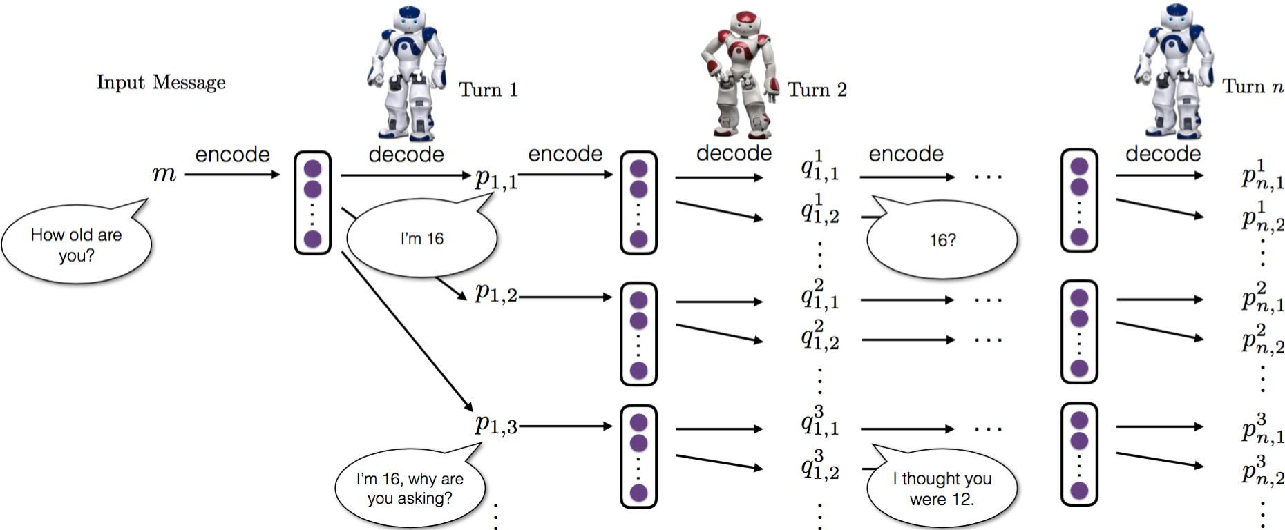
Figure 5.1: Dialogue simulation between the two agents.

Optimization

We initialize the policy model $p_{RL}$ with parameters from the mutual information model described in the previous subsection. We then use policy gradient methods to find parameters that lead to a larger expected reward. The objective to maximize is the expected future reward:

$$J_{RL}(\theta)=\mathbb{E}_{p_{RL}(a_{1:T})}\left[\sum_{i=1}^{i=T}R(a_{i},[p_{i},q_{i}])\right]$$ (5.8)

where $R(a_{i},[p_{i},q_{i}])$ denotes the reward resulting from action $a_{i}$. We use the likelihood ratio trick Williams (1992); Glynn (1990) for gradient updates:

$$\nabla J_{RL}(\theta)\approx{\sum_{i}\nabla\log p(a_{i}|p_{i},q_{i})}\sum_{i=1}^{i=T}R(a_{i},[p_{i},q_{i}])$$ (5.9)

5.2.4 Curriculum Learning

A curriculum learning strategy is again employed in which we begin by simulating the dialogue for 2 turns, and gradually increase the number of simulated turns. We generate 5 turns at most, as the number of candidates to examine grows exponentially in the size of the candidate list. Five candidate responses are generated at each step of the simulation.

In this section, we describe experimental results along with qualitative analysis. We evaluate dialogue generation systems using both human judgments and two automatic metrics: conversation length (number of turns in the entire session) and diversity.

5.3 Experiments

5.3.1 Dataset

The dialogue simulation requires high-quality initial inputs fed to the agent. For example, an initial input of “why ?” is undesirable since it is unclear how the dialogue could proceed. We take a subset of 10 million messages from the OpenSubtitles dataset and extract 0.8 million sequences with the lowest likelihood of generating the response “i don’t know what you are taking about” to ensure initial inputs are easy to respond to.

5.3.2 Automatic Evaluation

Evaluating dialogue systems is difficult. Metrics such as BLEU Papineni et al. (2002) and perplexity have been widely used for dialogue quality evaluation Li et al. (2016a); Vinyals and Le (2015); Sordoni et al. (2016), but it is widely debated how well these automatic metrics are correlated with true response quality Galley et al. (2015). Since the goal of the proposed system is not to predict the highest probability response, but rather the long-term success of the dialogue, we do not employ BLEU or perplexity for evaluation.

Length of the Dialogue

The first metric we propose is the length of the simulated dialogue. We say a dialogue ends when one of the agents starts generating dull responses such as “i don’t know” or two consecutive utterances from the same user are highly overlapping.

The test set consists of 1,000 input messages. To reduce the risk of circular dialogues, we limit the number of simulated turns to be less than 8. Results are shown in Table 5.2. As can be seen, using mutual information leads to more sustained conversations between the two agents. The proposed RL model is first trained based on the mutual information objective and thus benefits from it in addition to the RL model. We observe that the RL model with dialogue simulation achieves the best evaluation score.

Model	$\#$ of simulated turns
Seq2Seq	2.68
mutual information	3.40
RL	4.48

Table 5.2: The average number of simulated turns from standard Seq2Seq models, mutual information model and the proposed RL model.

Input Message	Mutual Information Model	RL
How old are you?	I’m 16.	I’m 16, why are you asking?
What’s your full name?	I have no idea.	What’s yours?
I don’t want to go home tonight.	Really?	Why?
Do you have any feelings for me?	I don’t know what you are talking about.	I don’t want to hurt your feelings.
How much time do you have here?	Not long enough. Sorry, sir.	Ten seconds.
Shall we get started?	Of course!	Yes. We’ve got a lot of work to do here.
Do you play football?	No, i don’t	Yes. I love football!
We’d have to talk to him.	I mean, he’s a good guy	About what ?
How come you never say it?	Because I don’t want to hurt you.	I don’t think it’s a good idea to say it.

Table 5.3: Sampled responses generated from the mutual information models and the proposed RL model.

Diversity

We report degree of diversity by calculating the number of distinct unigrams and bigrams in generated responses. The value is scaled by the total number of generated tokens to avoid favoring long sentences as described in Li et al. (2016a). The resulting metric is thus a type-token ratio for unigrams and bigrams.

For both the standard Seq2Seq model and the proposed RL model, we use beam search with a beam size 10 to generate a response to a given input message. For the mutual information model, we first generate $n$-best lists using $p_{{{\textsc{Seq2Seq}}}}(y|x)$ and then linearly re-rank them using $p_{{{\textsc{Seq2Seq}}}}(x|y)$. Results are presented in Table 5.4. We find that the proposed RL model generates more diverse outputs when compared against both the vanilla Seq2Seq model and the mutual information model.

Model	Unigram	Bigram
Seq2Seq	0.0062	0.015
mutual information	0.011	0.031
RL	0.017	0.041

Table 5.4: Diversity scores (type-token ratios) for the standard Seq2Seq model, mutual information model and the proposed RL model.

Human Evaluation

We explore three settings for human evaluation: the first setting is similar to what was described in Li et al. (2016a), where we employ crowdsourced judges to evaluate a random sample of 500 items. We present both an input message and the generated outputs to 3 judges and ask them to decide which of the two outputs is better (denoted as single-turn general quality). Ties are permitted. Identical strings are assigned the same score. We measure the improvement achieved by the RL model over the mutual information model by the mean difference in scores between the models.

For the second setting, judges are again presented with input messages and system outputs, and are asked to decide which of the two outputs is easier to respond to so that the conversation is able to continue (denoted as single-turn ease to answer). Again we evaluate a random sample of 500 items, each being assigned to 3 judges.

Title: Describe which response is easier to respond to (about 1 min)

Instructions:

In each task, you are given two dialogue episodes, each of which consists two dialogue turns. The first turns of the two episodes are the same. You need to decide the second turn of which dialogue episode is easier to respond to. Ties are permitted.

Each task will be assigned to three Turkers. We will give bonuses for those whose results for the same task are consistent.

Figure 5.2: Instructions given to turkers for the single-turn-ease-to-answer task.

For the third setting, judges are presented with simulated conversations between the two agents (denoted as multi-turn general quality). Each conversation consists of 5 turns. We evaluate 200 simulated conversations, each being assigned to 3 judges, who are asked to decide which of the simulated conversations is of higher quality.

Setting	RL-win	RL-lose	Tie
single-turn general quality	0.40	0.36	0.24
single-turn ease to answer	0.52	0.23	0.25
multi-turn general quality	0.72	0.12	0.16

Table 5.5: RL gains over the mutual information system based on pairwise human judgments.

Results for human evaluation are shown in Table 5.5. The proposed RL system does not introduce a significant boost in single-turn response quality (winning 40 percent of time and losing 36 percent of time). This is in line with our expectations, as the RL model is not optimized to predict the next utterance, but rather to increase long-term reward. The RL system produces responses that are significantly easier to answer than does the mutual information system, as demonstrated by the single-turn ease to answer setting (winning 52 percent of time and losing 23 percent of time), and also significantly higher quality multi-turn dialogues, as demonstrated by the multi-turn general quality setting (winning 72 percent of time).

Qualitative Analysis and Discussion

We show a random sample of generated responses in Table 5.3 and simulated conversations in Table 5.1 at the beginning of the paper. From Table 5.3, we can see that the RL based agent indeed generates more interactive responses than the other baselines. We also find that the RL model has a tendency to end a sentence with another question and hand the conversation over to the user. From Table 5.1, we observe that the RL model manages to produce more interactive and sustained conversations than the mutual information model.

During error analysis, we found that although we penalize repetitive utterances in consecutive turns, the dialogue sometimes enters a cycle with length greater than one, as shown in Table 5.6. This can be ascribed to the limited amount of conversational history we consider. Another issue observed is that the model sometimes starts a less relevant topic during the conversation. There is a tradeoff between relevance and less repetitiveness, as manifested in the reward function we defined.

A: What’s your name ?

B: Daniel.

A: How old are you ?

B. Twelve. What’s your name ?

A. Daniel.

B: How old are you ?

A: Twelve. What’s your name ?

B: Daniel.

A: How old are you ?

B …

Table 5.6: An simulated dialogue with a cycle longer than one.

The fundamental problem, of course, is that the manually defined reward function can’t possibly cover the crucial aspects that define an ideal conversation. While the heuristic rewards that we defined are amenable to automatic calculation, and do capture some aspects of what makes a good conversation, ideally the system would instead receive real rewards from humans. But such a strategy is both costly and hard to scale up. As we will describe in the following section, we can train a machine to act as the role of a human evaluator and provide reward signals to train the response generation model.

5.4 Conclusion

We introduce a reinforcement learning framework for neural response generation by simulating dialogues between two agents, integrating the strengths of neural Seq2Seq systems and reinforcement learning for dialogue. Like earlier neural Seq2Seq models, our framework captures the compositional models of the meaning of a dialogue turn and generates semantically appropriate responses. Like reinforcement learning dialogue systems, our framework is able to generate utterances that optimize future reward, successfully capturing global properties of a good conversation. Despite the fact that our model uses very simple, operationable heuristics for capturing these global properties, the framework generates more diverse, interactive responses that foster a more sustained conversation.

Chapter 6 Adversarial Learning for Dialogue Generation

In the previous chapter (chapter 5), we manually define three types of ideal dialogue properties, i.e., ease of answering, informativeness, and coherence, based on which a reinforcement learning system is trained. However, it is widely acknowledged that manually defined reward functions can’t possibly cover all crucial aspects and can lead to suboptimal generated utterances. This relates to two important questions in dialogue learning: what are the crucial aspects that define an ideal conversation and how can we quantitatively measure them.

A good dialogue model should generate utterances indistinguishable from human dialogues. Such a goal suggests a training objective resembling the idea of the Turing test Turing (1950). We borrow the idea of adversarial training Goodfellow et al. (2014); Denton et al. (2015) in computer vision, in which we jointly train two models, a generator (which takes the form of the neural Seq2Seq model) that defines the probability of generating a dialogue sequence, and a discriminator that labels dialogues as human-generated or machine-generated. This discriminator is analogous to the evaluator in the Turing test. We cast the task as a reinforcement learning problem, in which the quality of machine-generated utterances is measured by its ability to fool the discriminator into believing that it is a human-generated one. The output from the discriminator is used as a reward to the generator, pushing it to generate utterances indistinguishable from human-generated dialogues.

The idea of a Turing test—employing an evaluator to distinguish machine-generated texts from human-generated ones—can be applied not only to training but also testing, where it goes by the name of adversarial evaluation. Adversarial evaluation was first employed in Bowman et al. (2016) to evaluate sentence generation quality, and preliminarily studied in the context of dialogue generation by Kannan and Vinyals (2016). Here, we discuss potential pitfalls of adversarial evaluations and necessary steps to avoid them and make evaluation reliable.

Experimental results demonstrate that our approach produces more interactive, interesting, and non-repetitive responses than standard Seq2Seq models trained using the MLE objective function.

6.1 Adversarial Reinforcement Learning

In this section, we describe in detail the components of the proposed adversarial reinforcement learning model. The problem can be framed as follows: given a dialogue history $x$ consisting of a sequence of dialogue utterances, the model needs to generate a response $y=\{y_{1},y_{2},...,y_{L_{y}}\}$. We view the process of sentence generation as a sequence of actions that are taken according to a policy defined by an encoder-decoder recurrent neural networks.

6.1.1 Adversarial REINFORCE

The adversarial REINFORCE algorithm consists of two components: a generative model $G$ and a discriminative model $D$.

Generative Model

The generative model $G$ defines the policy that generates a response $y$ given dialogue history $x$. It takes a form similar to Seq2Seq models, which first map the source input to a vector representation using a recurrent net and then compute the probability of generating each token in the target using a softmax function.

Discriminative Model

The discriminative model $D$ is a binary classifier that takes as input a sequence of dialogue utterances $\{x,y\}$ and outputs a label indicating whether the input is generated by humans or machines. The input dialogue is encoded into a vector representation using a hierarchical encoder Li et al. (2015); Serban et al. (2016a), which is then fed to a 2-class softmax function, returning the probability of the input dialogue episode being a machine-generated dialogue (denoted $Q_{-}(\{x,y\})$) or a human-generated dialogue (denoted $Q_{+}(\{x,y\})$).

Policy Gradient Training

The key idea of the system is to encourage the generator to generate utterances that are indistinguishable from human generated dialogues. We use policy gradient methods to achieve such a goal, in which the score of current utterances being human-generated ones assigned by the discriminator (i.e., $Q_{+}(\{x,y\})$) is used as a reward for the generator, which is trained to maximize the expected reward of generated utterance(s) using the REINFORCE algorithm Williams (1992):

$$J(\theta)=\mathbb{E}_{y\sim p(y|x)}(Q_{+}(\{x,y\})|\theta)$$ (6.1)

Given the input dialogue history $x$, the bot generates a dialogue utterance $y$ by sampling from the policy. The concatenation of the generated utterance $y$ and the input $x$ is fed to the discriminator. The gradient of (6.1) is approximated using the likelihood ratio trick Williams (1992); Glynn (1990); aleksand1968stochastic:

$$\nabla J(\theta)\approx[Q_{+}(\{x,y\})-b(\{x,y\})]\\ \nabla\log\pi(y|x)\\ =[Q_{+}(\{x,y\})-b(\{x,y\})]\\ \nabla\sum_{t}\log p(y_{t}|x,y_{1:t-1})$$ (6.2)

where $\pi$ denotes the probability of the generated responses. $b(\{x,y\})$ denotes the baseline value to reduce the variance of the estimate while keeping it unbiased. The discriminator is simultaneously updated with the human generated dialogue that contains dialogue history $x$ as a positive example and the machine-generated dialogue as a negative example.

6.1.2 Reward for Every Generation Step (REGS)

The REINFORCE algorithm described has the disadvantage that the expectation of the reward is approximated by only one sample, and the reward associated with this sample (i.e., $[Q_{+}(\{x,y\})-b(\{x,y\})]$ in Eq(6.2)) is used for all actions (the generation of each token) in the generated sequence. Suppose, for example, the input history is what’s your name, the human-generated response is I am John, and the machine-generated response is I don’t know. The vanilla REINFORCE model assigns the same negative reward to all tokens within the human-generated response (i.e., I, don’t, know), whereas proper credit assignment in training would give separate rewards, most likely a neutral reward for the token I, and negative rewards to don’t and know. We call this reward for every generation step, abbreviated REGS.

Rewards for intermediate steps or partially decoded sequences are thus necessary. Unfortunately, the discriminator is trained to assign scores to fully generated sequences, but not partially decoded ones. We propose two strategies for computing intermediate step rewards by (1) using Monte Carlo (MC) search and (2) training a discriminator that is able to assign rewards to partially decoded sequences.

In (1) Monte Carlo search, given a partially decoded $s_{P}$, the model keeps sampling tokens from the distribution until the decoding finishes. Such a process is repeated $N$ (set to 5) times and the $N$ generated sequences will share a common prefix $s_{P}$. These $N$ sequences are fed to the discriminator, the average score of which is used as a reward for the $s_{P}$. A similar strategy is adopted in yu2016seqgan. The downside of MC is that it requires repeating the sampling process for each prefix of each sequence and is thus significantly time-consuming.

In (2), we directly train a discriminator that is able to assign rewards to both fully and partially decoded sequences. We break the generated sequences into partial sequences, namely $\{y^{+}_{1:t}\}_{t=1}^{N_{Y^{+}}}$ and $\{y^{-}_{1:t}\}_{t=1}^{N_{Y^{-}}}$ and use all instances in $\{y^{+}_{1:t}\}_{t=1}^{N_{Y^{+}}}$ as positive examples and instances $\{y^{-}_{1:t}\}_{t=1}^{N_{Y^{-}}}$ as negative examples. The problem with such a strategy is that earlier actions in a sequence are shared among multiple training examples for the discriminator (for example, token $y^{+}_{1}$ is contained in all partially generated sequences, which results in overfitting. To mitigate this problem, we adopt a strategy similar to when training value networks in AlphaGo Silver et al. (2016), in which for each collection of subsequences of $Y$, we randomly sample only one example from $\{y^{+}_{1:t}\}_{t=1}^{N_{Y^{+}}}$ and one example from $\{y^{-}_{1:t}\}_{t=1}^{N_{Y^{-}}}$, which are treated as positive and negative examples to update the discriminator. Compared with the Monte Carlo search model, this strategy is significantly more time-effective, but comes with the weakness that the discriminator becomes less accurate after partially decoded sequences are added in as training examples. We find that the MC model performs better when training time is less of an issue.

For each partially-generated sequence $Y_{t}=y_{1:t}$, the discriminator gives a classification score $Q_{+}(x,Y_{t})$. We compute the baseline $b(x,Y_{t})$ using a similar model to the vanilla REINFORCE model. This yields the following gradient to update the generator:

$$\nabla J(\theta)\approx\sum_{t}(Q_{+}(x,Y_{t})-b(x,Y_{t}))\\ \nabla\log p(y_{t}|x,Y_{1:t-1})$$ (6.3)

Comparing (6.3) with (6.2), we can see that the values for rewards and baselines are different among generated tokens in the same response.

Teacher Forcing

Practically, we find that updating the generative model only using Eq. 6.1 leads to unstable training for both vanilla Reinforce and REGS, with the perplexity value skyrocketing after training the model for a few hours (even when the generator is initialized using a pre-trained Seq2Seq model). The reason this happens is that the generative model can only be indirectly exposed to the gold-standard target sequences through the reward passed back from the discriminator, and this reward is used to promote or discourage its (the generator’s) own generated sequences. Such a training strategy is fragile: once the generator (accidentally) deteriorates in some training batches and the discriminator consequently does an extremely good job in recognizing sequences from the generator, the generator immediately gets lost. It knows that its generated sequences are bad based on the rewards outputted from the discriminator, but it does not know what sequences are good and how to push itself to generate these good sequences (the odds of generating a good response from random sampling are minute, due to the vast size of the space of possible sequences). Loss of the reward signal leads to a breakdown in the training process.

To alleviate this issue and give the generator more direct access to the gold-standard targets, we propose also feeding human generated responses to the generator for model updates. The most straightforward strategy is for the discriminator to automatically assign a reward of 1 (or other positive values) to the human generated responses and for the generator to use this reward to update itself on human generated examples. This can be seen as having a teacher intervene with the generator some fraction of the time and force it to generate the true responses, an approach that is similar to the professor-forcing algorithm of lamb2016professor.

A closer look reveals that this modification is the same as the standard training of Seq2Seq models, making the final training alternately update the Seq2Seq model using the adversarial objective and the MLE objective. One can think of the professor-forcing model as a regularizer to regulate the generator once it starts deviating from the training dataset.

We also propose another workaround, in which the discriminator first assigns a reward to a human generated example using its own model, and the generator then updates itself using this reward on the human generated example only if the reward is larger than the baseline value. Such a strategy has the advantage that different weights for model updates are assigned to different human generated examples (in the form of different reward values produced by the generator) and that human generated examples are always associated with non-negative weights.

A review of the proposed model is shown in Figure 6.1.

Figure 6.1: A brief review of the proposed adversarial reinforcement algorithm for training the generator $G$ and discriminator $D$. The reward $r$ from the discriminator $D$ can be computed using different strategies according to whether using REINFORCE or REGS. The update of the generator $G$ on $(X,\hat{Y})$ can be done by either using Eq.6.2 or Eq.6.3. D-steps is set to 5 and G-steps is set to 1.

6.1.3 Training Details

We first pre-train the generative model by predicting target sequences given the dialogue history. We trained a Seq2Seq model Sutskever et al. (2014) with an attention mechanism Bahdanau et al. (2014); Luong et al. (2015b) on the OpenSubtitles dataset. We followed protocols recommended by Sutskever et al. (2014), such as gradient clipping, mini-batch, and learning rate decay. We also pre-train the discriminator. To generate negative examples, we decode part of the training data. Half of the negative examples are generated using beam-search with mutual information reranking as described in Li et al. (2016a), and the other half is generated from sampling.

For data processing, model training, and decoding (both the proposed adversarial training model and the standard Seq2Seq models), we employ a few strategies that improve response quality, including: (1) Remove training examples with the length of responses shorter than a threshold (set to 5). We find that this significantly improves the general response quality. (2) Instead of using the same learning rate for all examples, using a weighted learning rate that considers the average tf-idf score for tokens within the response. Such a strategy decreases the influence from dull and generic utterances. (3) Penalizing intra-sibling ranking when doing beam search decoding to promote N-best list diversity as described in Chapter 3. (4) Penalizing word types (stop words excluded) that have already been generated. Such a strategy dramatically decreases the rate of repetitive responses such as no. no. no. no. no. or contradictory responses such as I don’t like oranges but i like oranges.

6.2 Adversarial Evaluation

In this section, we discuss details of strategies for successful adversarial evaluation. It is worth noting that the proposed adversarial training and adversarial evaluation are separate procedures.They are independent of each other and share no common parameters.

The idea of adversarial evaluation, first proposed by Bowman et al. (2016), is to train a discriminant function to separate generated and true sentences, in an attempt to evaluate the model’s sentence generation capability. The idea has been preliminarily studied by Kannan and Vinyals (2016) in the context of dialogue generation. Adversarial evaluation also resembles the idea of the Turing test, which requires a human evaluator to distinguish machine-generated texts from human-generated ones. Since it is time-consuming and costly to ask a human to talk to a model and give judgements, we train a machine evaluator in place of the human evaluator to distinguish the human dialogues and machine dialogues, and we use it to measure the general quality of the generated responses.

Adversarial evaluation involves both training and testing. At training time, the evaluator is trained to label dialogues as machine-generated (negative) or human-generated (positive). At test time, the trained evaluator is evaluated on a held-out dataset. If the human-generated dialogues and machine-generated ones are indistinguishable, the model will achieve 50 percent accuracy at test time.

6.2.1 Adversarial Success

We define Adversarial Success (AdverSuc for short) to be the fraction of instances in which a model is capable of fooling the evaluator. AdverSuc is the difference between 1 and the accuracy achieved by the evaluator. Higher values of AdverSuc for a dialogue generation model are better.

6.2.2 Testing the Evaluator’s Ability

One caveat with the adversarial evaluation methods is that they are model-dependent. We approximate the human evaluator in the Turing test with an automatic evaluator and assume that the evaluator is perfect: low accuracy of the discriminator should indicate high quality of the responses, since we interpret this to mean the generated responses are indistinguishable from the human ones. Unfortunately, there is another factor that can lead to low discriminative accuracy: a poor discriminative model. Consider a discriminator that always gives random labels or always gives the same label. Such an evaluator always yields a high AdverSuc value of 0.5. Bowman et al. (2016) propose two different discriminator models separately using unigram features and neural features. It is hard to tell which feature set is more reliable. The standard strategy of testing the model on a held-out development set is not suited to this case, since a model that overfits the development set is necessarily superior.

To deal with this issue, we propose setting up a few manually-invented situations to test the ability of the automatic evaluator. This is akin to setting up examinations to test the ability of the human evaluator in the Turing test. We report not only the AdverSuc values, but also the scores that the evaluator achieves in these manually-designed test cases, indicating how much we can trust the reported AdverSuc. We develop scenarios in which we know in advance how a perfect evaluator should behave, and then compare AdverSuc from a discriminative model with the gold-standard AdverSuc. Scenarios we design include:

• We use human-generated dialogues as both positive examples and negative examples. A perfect evaluator should give an AdverSuc of $0.5$ (accuracy $50\%$), which is the gold-standard result.

• We use machine-generated dialogues as both positive examples and negative examples. A perfect evaluator should give an AdverSuc of $0.5$ (accuracy $50\%$).

• We use original human-generated dialogues as positive examples and dialogues consisting of random utterances as negative examples. A perfect evaluator should give an AdverSuc of $0$ (accuracy $100\%$).

• We use original human-generated dialogues as positive examples and dialogues with responses replaced by the utterances immediately following the true responses. A perfect evaluation should give an AdverSuc of $0$ (accuracy $100\%$).

The evaluator reliability error (ERE) is the average deviation of an evaluator’s adversarial error from the gold-standard error in the above tasks, with equal weight for each task. The smaller the error, the more reliable the evaluator is.

Input	tell me … how long have you had this falling sickness ?
Vanilla-MLE	i ’m not a doctor .
Vanilla-Sample	well everything you did was totally untrue .
REINFORCE	i don ’t know how long it ’s been .
REGS Monte Carlo	A few months, I guess .
Input	so i had the doctors test sammy ’s response to conditioning .
Vanilla-MLE	sammy wrote the test sammy wrote the test .
Vanilla-Sample	objects pick objects up objects objects objects objects objects
REINFORCE	i ’m not sure that ’s relevant .
REGS Monte Carlo	so he took the pills .
Input	what are you going to do ?
Vanilla-MLE	i ’m going to the movies .
Vanilla-Sample	get him outta here first !
REINFORCE	i ’m going to get you .
REGS Monte Carlo	i ’m going to get you a new car .
Input	they fear your power your intellect .
Vanilla-MLE	you ’re the only one who knows what ’s going on .
Vanilla-Sample	when they are conquered and you surrender they will control all of us .
REINFORCE	i ’m afraid i ’m not ready yet .
REGS Monte Carlo	i ’m not afraid of your power .

Table 6.1: Sampled responses from different models. More in Appendix Tables 6.5 and 6.6.

6.2.3 Machine-vs-Random Accuracy

Evaluator reliability error uses scenarios constructed from human-generated dialogues to assess feature or hyper-parameter choice for the evaluator. Unfortunately, no machine-generated responses are involved in the ERE metric. The following example illustrates the serious weakness resulting from this strategy: as will be shown in the experiment section, when inputs are decoded using greedy or beam search models, most generation systems to date yield an adversarial success less than 10 percent (evaluator accuracy 90 percent). But when using sampling for decoding, the adversarial success skyrockets to around 40 percent, only 10 percent less than what’s needed to pass the Turing test. A close look at the decoded sequences using sampling tells a different story: the responses from sampling are sometimes incoherent, irrelevant or even ungrammatical.

We thus propose an additional sanity check, in which we report the accuracy of distinguishing between machine-generated responses and randomly sampled responses (machine-vs-random for short). This resembles the N-choose-1 metric described in shao15. Higher accuracy indicates that the generated responses are distinguishable from randomly sampled human responses, indicating that the generative model is not fooling the generator simply by introducing randomness. As we will show in Sec. 6.3, using sampling results in high AdverSuc values but low machine-vs-random accuracy.

6.3 Experimental Results

In this section, we detail experimental results on adversarial success and human evaluation.

Setting	ERE
SVM+Unigram	0.232
Concat Neural	0.209
Hierarchical Neural	0.193
SVM+Neural+multil-features	0.152

Table 6.2: ERE scores obtained by different models.

6.3.1 Adversarial Evaluation

ERE

We first test adversarial evaluation models with different feature sets and model architectures for reliability, as measured by evaluator reliability error (ERE). We explore the following models: (1) SVM+Unigram: SVM using unigram features. A multi-utterance dialogue (i.e., input messages and responses) is transformed to a unigram representation; (2) Concat Neural: a neural classification model with a softmax function that takes as input the concatenation of representations of constituent dialogues sentences; (3) Hierarchical Neural: a hierarchical encoder with a structure similar to the discriminator used in the reinforcement; and (4) SVM+Neural+multi-lex-features: a SVM model that uses the following features: unigrams, neural representations of dialogues obtained by the neural model trained using strategy (3), the forward likelihood $\log p(y|x)$ and backward likelihood $p(x|y)$.

ERE scores obtained by different models are reported in Table 6.2. As can be seen, the hierarchical neural evaluator (model 3) is more reliable than simply concatenating the sentence-level representations (model 2). Using the combination of neural features and lexicalized features yields the most reliable evaluator. For the rest of this section, we report results obtained by the hierarchical Neural setting due to its end-to-end nature, despite its inferiority to SVM+Neural+multil-features.

Table 6.3 presents AdverSuc values for different models, along with machine-vs-random accuracy described in Section 4.3. Higher values of AdverSuc and machine-vs-random are better.

Baselines we consider include standard Seq2Seq models using greedy decoding (MLE-greedy), beam-search (MLE+BS) and sampling, as well as the mutual information reranking model (as described in Chapter 3) with two algorithmic variations: (1) MMI+$p(y|x)$, in which a large N-best list is first generated using a pre-trained Seq2Seq model and then reranked by the backward probability $p(x|y)$ and (2) MMI$-p(y)$, in which language model probability is penalized during decoding.

Results are shown in Table 6.3. What first stands out is decoding using sampling (as discussed in Section 4.3), achieving a significantly higher AdverSuc number than all the rest models. However, this does not indicate the superiority of the sampling decoding model, since the machine-vs-random accuracy is at the same time significantly lower. This means that sampled responses based on Seq2Seq models are not only hard for an evaluator to distinguish from real human responses, but also from randomly sampled responses. A similar, though much less extreme, effect is observed for MMI$-p(y)$, which has an AdverSuc value slightly higher than Adver-Reinforce, but a significantly lower machine-vs-random score.

By comparing different baselines, we find that MMI+$p(y|x)$ is better than MLE-greedy, which is in turn better than MLE+BS. This result is in line with human-evaluation results from Li et al. (2016a). The two proposed adversarial algorithms achieve better performance than the baselines. We expect this to be the case, since the adversarial algorithms are trained on an objective function more similar to the the evaluation metric (i.e., adversarial success). REGS performs slightly better than the vanilla REINFORCE algorithm.

Model	AdverSuc	machine-vs-random
MLE-BS	0.037	0.942
MLE-Greedy	0.049	0.945
MMI+$p(t|s)$	0.073	0.953
MMI-$p(t)$	0.090	0.880
Sampling	0.372	0.679
Adver-Reinforce	0.080	0.945
Adver-REGS	0.098	0.952

Table 6.3: AdverSuc and machine-vs-random scores achieved by different training/decoding strategies.

6.3.2 Human Evaluation

For human evaluation, we follow protocols defined in Chapter 5, employing crowdsourced judges to evaluate a random sample of 200 items. We present both an input message and the generated outputs to 3 judges and ask them to decide which of the two outputs is better (single-turn general quality). They were instructed to prefer outputs that were more specific (relevant) to the message and preceding context, Ties are permitted. Identical strings are assigned the same score. We also present the judges with multi-turn conversations simulated between the two agents. Each conversation consists of 3 turns. Results are presented in Table 6.4. We observe a significant quality improvement on both single-turn quality and multi-turn quality from the proposed adversarial model. It is worth noting that the reinforcement learning system described in Chapter 5, which simulates conversations between two bots and is trained based on manually designed reward functions, only improves multi-turn dialogue quality, while the model described in this chapter improves both single-turn and multi-turn dialogue generation quality. This confirms that the reward adopted in adversarial training is more general, natural, and effective in training dialogue systems.

Setting	adver-win	adver-lose	tie
single-turn	0.62	0.18	0.20
multi-turn	0.72	0.10	0.18

Table 6.4: The gain from the proposed adversarial model over the mutual information system based on pairwise human judgments.

Input	maybe his eyes were too big for his stomach .
Vanilla-MLE	he ’s got a big mouth .
Vanilla-Sample	i ’m sure he ’s unhappy with the fact .
Reinforce	he ’s a little bit of a pain .
MC	i don ’t think so .
Input	they didn ’t have much success with this problem commander .
Vanilla-MLE	they ’re not the only ones who have been in the system .
Vanilla-Sample	it ’s the new priority only .
Reinforce	they ’re not the only ones who can help us .
MC	can we find someone else ?
Input	and he carried them all the time wherever he went .
Vanilla-MLE	i don ’t know who he is .
Vanilla-Sample	the church … suffered the winds of 900 meters with horse aid .
Reinforce	he was a good man .
MC	he was a very good man .
Input	somebody probably flushed their pet snake down the toilet .
Vanilla-MLE	i ’m sure the dog will be here soon .
Vanilla-Sample	i could at least think .
Reinforce	i don ’t think so .
MC	i don ’t think so .
Input	excuse me but how did we pay for these suits ?
Vanilla-MLE	i ’m not a beggar .
Vanilla-Sample	is this the money eugene ?
Reinforce	i don ’t know what to do .
MC	how much money you owe me ?
Input	… while the beautiful and happy world was madly destroyed ;
Vanilla-MLE	i was born in the world of the world
Vanilla-Sample	as in childhood i took you to one tenth of a postcard
Reinforce	and the world was full of joy .
MC	and the world was full of joy .
Input	i was kinda hoping that you were my dad .
Vanilla-MLE	i ’m just a little bit of a little bit of a little bit of a little bit of a
Vanilla-Sample	shiny gold gold and silver in the mountains .
Reinforce	i ’m not gonna be a baby .
MC	i ’m not going to be a father .
Input	the man who does that is not afraid to die .
Vanilla-MLE	he ’s not afraid of the dark .
Vanilla-Sample	even the program is the only truth
Reinforce	he ’s also not afraid of me .
MC	he ’s such a brave man !

Table 6.5: Sampled responses outputted from different models

Input	i ’ll have to drive home .
Vanilla-MLE	i ’ll be back in a minute .
Vanilla-Sample	let ’s go for some fun .
Reinforce	i ’ll drive you home .
MC	i don ’t have a car .
Input	i had to work late and then i went for a walk .
Vanilla-MLE	i was in the middle of the road .
Vanilla-Sample	my body was just pounding .
Reinforce	i was just trying to help you .
MC	i was just trying to get a little sleep .
Input	lots of cream lots of sugar .
Vanilla-MLE	i ’m gonna be in the kitchen .
Vanilla-Sample	was this gay or red ?
Reinforce	i don ’t want to be a vegetable .
MC	i ’m not a very good cook .
Input	so they just let him go ?
Vanilla-MLE	he ’s not gonna let them go through the motions .
Vanilla-Sample	they asked him whether we could go see ernesto ?
Reinforce	i don ’t know what to do .
MC	he ’s not going to be here any longer .
Input	you must not bomb this town .
Vanilla-MLE	you have to go back to the city .
Vanilla-Sample	the one is a multiple choice .
Reinforce	I think I have to .
MC	I think I have to .
Input	communism recently failed in eastern europe .
Vanilla-MLE	the war is not over .
Vanilla-Sample	there are people who hope that in tokyo they won ’t risk losing their departing .
Reinforce	and the people who are not the same .
MC	the war is still going on .
Input	you should stop in more often .
Vanilla-MLE	I don ’t think so .
Vanilla-Sample	is it possible as old as you ?
Reinforce	i ’m not going to be a burden on you .
MC	i don ’t want to be a burden .
Input	he couldn ’t have heard us .
Vanilla-MLE	he was in the middle of the night .
Vanilla-Sample	he should have been somewhere out here .
Reinforce	he ’s not a good guy .
MC	he ’s got a lot of nerve.
Input	that ’s our wake up call .
Vanilla-MLE	we ’re gonna be late for the meeting .
Vanilla-Sample	c ’mon c ’mon let ’s get outta here .
Reinforce	i ’ll be right back .
MC	we ’re gonna have to get to the station .

Table 6.6: Sampled responses outputted from different models

6.4 Conclusion

In this chapter, drawing intuitions from the Turing test, we propose using an adversarial training approach for response generation. We cast the model in the framework of reinforcement learning and train a generator based on the signal from a discriminator to generate response sequences indistinguishable from human-generated dialogues. We observe clear performance improvements on multiple metrics from the adversarial training strategy.

Chapter 7 Learning by Asking Questions

In the two chapters below, our focus switches from the chit-chat systems to interactive QA dialogue systems. We will talk about how we can design an interactive dialogue agent, and how this agent can benefit from interacting with humans. The reason why we choose to study the issues with human-bot interactions under the context of factoid QA is because it is easier to formalize the problem and evaluate various aspects of features and performances in a more domain-specific QA task. But chit-chat systems and interactive QA systems are closely related and the methodology we proposed in this chapter is a general one: a chit-chat dialogue system can certainly benefit from the types of interactions that will be studied in the two chapters below.

In this chapter, we will discuss how we can train a bot to ask questions. Think about the following situation: when a student is asked a question by a teacher, but is not confident about the answer, they may ask for clarification or hints. A good conversational agent should have this ability to interact with a dialogue partner (the teacher/user). However, recent efforts have mostly focused on learning through fixed answers provided in the training set, rather than through interactions. In that case, when a learner encounters a confusing situation such as an unknown surface form (phrase or structure), a semantically complicated sentence or an unknown word, the agent will either make a (usually poor) guess or will redirect the user to other resources (e.g., a search engine, as in Siri). Humans, in contrast, can adapt to many situations by asking questions.

In this chapter, we study this issue in the context of a knowledge-base based question answering task, where the dialogue agent has access to a knowledge base (KB) and need to answer a question based on the KB. We first identify three categories of mistakes a learner can make during a question-answering based dialogue scenario: (1) the learner has problems understanding the surface form of the text of the dialogue partner, e.g., the phrasing of a question; (2) the learner has a problem with reasoning, e.g., they fail to retrieve and connect the relevant knowledge to the question at hand; (3) the learner lacks the knowledge necessary to answer the question in the first place – that is, the knowledge sources the student has access to do not contain the needed information.

All the situations above can be potentially addressed through interaction with the dialogue partner. Such interactions can be used to learn to perform better in future dialogues. If a human student has problems understanding a teacher’s question, they might ask the teacher to clarify the question. If the student doesn’t know where to start, they might ask the teacher to point out which known facts are most relevant. If the student doesn’t know the information needed at all, they might ask the teacher to tell them the knowledge they’re missing, writing it down for future use.

In this work, we try to bridge the gap between how a human and an end-to-end machine learning dialogue agent deal with these situations: our student has to learn how to learn. We hence design a simulator and a set of synthetic tasks in the movie question answering domain that allow a bot to interact with a teacher to address the issues described above. Using this framework, we explore how a bot can benefit from interaction by asking questions in both offline supervised settings and online reinforcement learning settings, as well as how to choose when to ask questions in the latter setting. In both cases, we find that the learning system improves through interacting with users.

Finally, we validate our approach on real data where the teachers are humans using Amazon Mechanical Turk, and observe similar results.

7.1 Tasks

In this section we describe the dialogue tasks we designed. They are tailored for the three different situations described in Section 1 that motivate the bot to ask questions: (1) Question Clarification, in which the bot has problems understanding its dialogue partner’s text; (2) Knowledge Operation, in which the bot needs to ask for help to perform reasoning steps over an existing knowledge base; and (3) Knowledge Acquisition, in which the bot’s knowledge is incomplete and needs to be filled.

For our experiments we adapt the WikiMovies dataset (Weston et al., 2016), which consists of roughly 100k questions over 75k entities based on questions with answers in the open movie dataset (OMDb). The training/dev/test sets respectively contain 181638 / 9702 / 9698 examples. The accuracy metric corresponds to the percentage of times the student gives correct answers to the teacher’s questions.

Each dialogue takes place between a teacher and a bot. In this section we describe how we generate tasks using a simulator. Section 7.2.2 discusses how we test similar setups with real data using Mechanical Turk.

The bot is first presented with facts from the OMDb KB. This allows us to control the exact knowledge the bot has access to. Then, we include several teacher-bot question-answer pairs unrelated to the question the bot needs to answer, which we call conversation histories. In order to explore the benefits of asking clarification questions during a conversation, for each of the three scenarios, our simulator generated data for two different settings, namely, Question-Answering (denoted by QA) and Asking-Question (denoted by AQ). For both QA and AQ, the bot needs to give an answer to the teacher’s original question at the end.

7.1.1 Question Clarification.

The QA-based dialogue system is interactive Rieser and Lemon (2009): instead of just having to answer one single question, the QA-based system needs the ability to handle a diverse category of interaction-related issues such as asking for question clarification Stoyanchev et al. (2013, 2014), adapting answers given a human’s feedback Rieser and Lemon (2009), self-learning when encountering new questions or concepts Purver (2006), etc. To handle these issues, the system needs to take proper actions based on the current conversation state, which resembles the key issue addressed in the state-based dialogue system.

As discussed in the previous sections, the bot needs to ask the teacher to clarify the question when it does not understand it. Actually, the task of ask for clarification has been studied in a variety of speech recognition scenarios when a speech recognition system fails to understand a user’s utterance, such as use the generic dialog act REJECT and emit a rule-based “Please repeat”, or “I don’t understand what you said” utterance, or generate more complicated targeted utterances in different clarification senarios Purver (2004); Nerbonne (2005); Stoyanchev and Johnston (2015).

In this setting, the bot does not understand the teacher’s question. We focus on a special situation where the bot does not understand the teacher because of typo/spelling mistakes, as shown in Figure 7.1. We intentionally misspell some words in the questions such as replacing the word “movie” with “movvie” or “star” with “sttar”. To make sure that the bot will have problems understanding the question, we guarantee that the bot has never encountered the misspellings before—the misspelling-introducing mechanisms in the training, dev, and test sets are different, so the same word will be misspelled in different ways in different sets. We present two AQ tasks: (i) Question Paraphrase where the student asks the teacher to use a paraphrase that does not contain spelling mistakes to clarify the question by asking “what do you mean?”; and (ii) Question Verification where the student asks the teacher whether the original typo-bearing question corresponds to another question without the spelling mistakes (e.g., “Do you mean which film did Tom Hanks appear in?”). The teacher will give feedback by giving a paraphrase of the original question without spelling mistakes (e.g., “I mean which film did Tom Hanks appear in”) in Question Paraphrase or positive/negative feedback in Question Verification. Next the student will give an answer and the teacher will give positive/negative feedback depending on whether the student’s answer is correct. Positive and negative feedback are variants of “No, that’s incorrect” or “Yes, that’s right”. In these tasks, the bot has access to all relevant entries in the KB.

7.1.2 Knowledge Operation

The bot has access to all the relevant knowledge (facts) but lacks the ability to perform necessary reasoning operations over them; see Figure 7.2. We focus on a special case where the bot will try to understand what are the relevant facts. We explore two settings: Ask For Relevant Knowledge (Task 3) where the bot directly asks the teacher to point out the relevant KB fact and Knowledge Verification (Task 4) where the bot asks whether the teacher’s question is relevant to one particular KB fact. The teacher will point out the relevant KB fact in the Ask For Relevant Knowledge setting or give a positive or negative response in the Knowledge Verification setting. Then the bot will give an answer to the teacher’s original question and the teacher will give feedback on the answer.

Task 1: Question Paraphrase (QA)		Task 1: Question Paraphrase (AQ):
kb: Larry Crowne directed_by Tom Hanks		kb: Larry Crowne directed_by Tom Hanks
kb: Forrest Gump starred_actors Tom Hanks,		kb: Forrest Gump starred_actors Tom Hanks,
Robin Wright, Gary Sinise		Robin Wright, Gary Sinise
kb: Forrest Gump directed_by Robert Zemeckis		kb: Forrest Gump directed_by Robert Zemeckis
T/S : Conversation History.		T/S : Conversation History.
T : Which movvie did Tom Hanks sttar in ?		T : Which movvie did Tom Hanks sttar in ?
S : Larry Crowne		S : What do you mean ?
T : Wrong. (-)		T : I mean which film did Tom Hanks appear in.
		T : Which movvie did Tom Hanks sttar in ?
		S : Forrest Gump
		T : That’s correct. (+)
Task 2: Question Verification (QA):		Task 2: Question Verification (AQ)
kb: Larry Crowne directed_by Tom Hanks		kb: Larry Crowne directed_by Tom Hanks
kb: Forrest Gump starred_actors Tom Hanks,		kb: Forrest Gump starred_actors Tom Hanks,
Robin Wright, Gary Sinise		Robin Wright, Gary Sinise
kb: Forrest Gump directed_by Robert Zemeckis		kb: Forrest Gump directed_by Robert Zemeckis
T/S : Conversation History.		T/S : Conversation History.
T : Which movvie did Tom Hanks sttar in ?		T : Which movvie did Tom Hanks sttar in ?
S : Forrest Gump		S : Do you mean which film did Tom Hanks appear in ?
T : That’s correct. (+)		T : That’s correct. (+)
		T : Which movvie did Tom Hanks sttar in ?
		S : Larry Crowne
		T : Sorry, that’s not right. (-)

Figure 7.1: Sample dialogues for the two Question Clarification tasks (rows) using both the traditional QA setting (left column) and AQ setting (right column). In each case the same example is given for simplicity. Black text prefixed by “kb:” denotes KB knowledge that the student has access to. Blue text is spoken by the teacher, denoted by T. (+) denotes a reward of 1 (and 0 otherwise) that the teacher assigns to the bot. Red text denotes responses or questions posed by the bot, denoted by S. Brown denotes typos deliberately introduced by the authors. For the Question Verification setting, the student can either ask a correct (pertinent) question (as in this example) or an incorrect (irrelevant) one. The teacher will give positive or negative feedback based on the correctness of the student’s question. In our offline superised learning experiments, the probability of asking pertinent questions and correctly answering the original question from the teacher is set to 0.5. Finally, T/S denotes 5 pairs of questions and answers that are irrelevant to the rest of the conversation.

Task 3: Ask For Relevant Knowledge (AQ):		Task 4: Knowledge Verification (AQ):
kb: Larry Crowne directed_by Tom Hanks		kb: Larry Crowne directed_by Tom Hanks
kb: Forrest Gump starred_actors Tom Hanks,		kb: Forrest Gump starred_actors Tom Hanks,
Robin Wright, Gary Sinise		Robin Wright, Gary Sinise
kb: Forrest Gump directed_by Robert Zemeckis		kb: Forrest Gump directed_by Robert Zemeckis
T/S : Conversation History.		T/S : Conversation History.
T : Which movie did Tom Hanks star in ?		T : Which movie did Tom Hanks star in ?
S : Can you give me a hint ?		S : Does it have something to do with
T : It is related to the kb fact that		Larry Crowne directed_by Tom Hanks?
Forrest Gump starred_actors Tom Hanks		T : No. That’s wrong. (-)
Robin Wright, Gary Sinise		T : Which movie did Tom Hanks star in ?
T : Which movie did Tom Hanks star in ?		S : Forrest Gump
S : Forrest Gump		T : That’s correct. (+)
T : That’s correct. (+)

Figure 7.2: Sample dialogues for Knowledge Operation tasks.

.
Task 5: Missing Question Entity (QA)		Task 5: Missing Question Entity (AQ)
$\mathcal{t}$kb: Larry Crowne directed_by Tom Hanks		$\mathcal{t}$kb: Larry Crowne directed_by Tom Hanks
$\mathcal{t}$kb: Forrest Gump starred_actors Tom Hanks		$\mathcal{t}$kb: Forrest Gump starred_actors Tom Hanks,
kb: Forrest Gump starred_actors Sally Field		kb: Forrest Gump starred_actors Sally Field
kb: Forrest Gump directed_by Robert Zemeckis		kb: Forrest Gump directed_by Robert Zemeckis
T/S : Conversation History.		T : Which movie did Tom Hanks star in ?
T : Which movie did Tom Hanks star in ?		S : I don’t know. What’s the answer?
S : Forrest Gump		T : The answer is Forrest Gump.
T : That’s correct. (+)		T/S : Conversation History.
		T : Which movie did Tom Hanks star in ?
		S : Forrest Gump
		T : That’s correct. (+)

Task 6: Missing Answer Entity (AQ)		Task 7: Missing Relation Entity (AQ)
kb: Larry Crowne directed_by Tom Hanks		kb: Larry Crowne directed_by Tom Hanks
$\mathcal{t}$kb: Forrest Gump starred_actors Tom Hanks		$\mathcal{t}$kb: Forrest Gump starred_actors Tom Hanks,
$\mathcal{t}$kb: Forrest Gump starred_actors Sally Field		$\mathcal{t}$kb: Forrest Gump starred_actors Sally Field
$\mathcal{t}$kb: Forrest Gump directed_by Robert Zemeckis		kb: Forrest Gump directed_by Robert Zemeckis
T : Which movie did Tom Hanks star in ?		T : Which movie did Tom Hanks star in ?
S : I don’t know. What’s the answer?		S : I don’t know. What’s the answer?
T : The answer is Forrest Gump.		T : The answer is Forrest Gump.
T/S : Conversation History.		T/S : Conversation History.
T : Which movie did Tom Hanks star in ?		T : Which movie did Tom Hanks star in ?
S : Forrest Gump		S : Forrest Gump
T : That’s correct. (+)		T : That’s correct. (+)

.
Task 8: Missing Triple (AQ)		Task 9: Missing Everything (AQ)
kb: Larry Crowne directed_by Tom Hanks		$\mathcal{t}$kb: Larry Crowne directed_by Tom Hanks
$\mathcal{t}$kb: Forrest Gump starred_actors Tom Hanks		$\mathcal{t}$kb: Forrest Gump starred_actors Tom Hanks,
kb: Forrest Gump starred_actors Sally Field		$\mathcal{t}$kb: Forrest Gump starred_actors Sally Field
kb: Forrest Gump directed_by Robert Zemeckis		$\mathcal{t}$kb: Forrest Gump directed_by Robert Zemeckis
T : Which movie did Tom Hanks star in ?		T : Which movie did Tom Hanks star in ?
S : I don’t know. What’s the answer?		S : I don’t know. What’s the answer?
T : The answer is Forrest Gump.		T : The answer is Forrest Gump.
T/S : Conversation History.		T/S : Conversation History.
T : Which movie did Tom Hanks star in ?		T : Which movie did Tom Hanks star in ?
S : Forrest Gump		S : Forrest Gump
T : That’s correct. (+)		T : That’s correct. (+)

Figure 7.3: Different tasks for Knowledge Acquisition. Crossed lines correspond to entries of the KB whose retrieval is missed.

7.1.3 Knowledge Acquisition

For the tasks in this subsection, the bot has an incomplete KB and there are entities important to the dialogue missing from it, see Figure 7.3. For example, given the question “Which movie did Tom Hanks star in?”, the missing part could either be the entity that the teacher is asking about (question entity for short, which is Tom Hanks in this example), the relation entity (starred_actors), the answer to the question (Forrest Gump), or the combination of the three. In all cases, the bot has little chance of giving the correct answer due to the missing knowledge. It needs to ask the teacher the answer to acquire the missing knowledge. The teacher will give the answer and then move on to other questions (captured in the conversational history). They later will come back to reask the question. At this point, the bot needs to give an answer since the entity is not new any more.

Though the correct answer has effectively been included in the earlier part of the dialogue as the answer to the bot’s question, as we will show later, many of the tasks are not as trivial as they look when the teacher reasks the question. This is because the bot’s model needs to memorize the missing entity and then construct the links between the missing entities and known ones. This is akin to the real world case where a student might make the same mistake again and again even though each time the teacher corrects them if their answer is wrong. We now detail each task in turn.

Missing Question Entity: The entity that the teacher is asking about is missing from the knowledge base. All KB facts containing the question entity will be hidden from the bot. In the example for Task 5 in Figure 7.3, since the teacher’s question contains the entity Tom Hanks, the KB facts that contain Tom Hanks are hidden from the bot.

Missing Answer Entity: The answer entity to the question is unknown to the bot. All KB facts that contain the answer entity will be hidden. Hence, in Task 6 of Figure 7.3, all KB facts containing the answer entity Forrest Gump will be hidden from the bot.

Missing Relation Entity: The relation type is unknown to the bot. In Task 7 of Figure 7.3, all KB facts that express the relation starred actors are hidden from the bot.

Missing Triples: The triple that expresses the relation between the question entity and the answer entity is hidden from the bot. In Task 8 of Figure 7.3, the triple “Forrest Gump (question entity) starred_actors Tom Hanks (answer entity)” will be hidden.

Missing Everything: The question entity, the relation entity, the answer entity are all missing from the KB. All KB facts in Task 9 of Figure 7.3 will be removed since they either contain the relation entity (i.e., starred_actors), the question entity (i.e., Forrest Gump) or the answer entity Tom Hanks.

7.2 Train/Test Regime

We now discuss in detail the regimes we used to train and test our models, which are divided between evaluation within our simulator and using real data collected via Mechanical Turk.

7.2.1 Simulator

Using our simulator, our objective was twofold. We first wanted to validate the usefulness of asking questions in all the settings described in the previous section. Second, we wanted to assess the ability of our student bot to learn when to ask questions. In order to accomplish these two objectives we explored training our models with our simulator using two methodologies, namely, Offline Supervised Learning and Online Reinforcement Learning.

Dialogue Simulator

Here we detail the simulator and the datasets we generated in order to realize the various scenarios discussed in Section 7.1. We focused on the problem of movieQA where we adapted the WikiMovies dataset proposed in Weston et al. (2016). The dataset consists of roughly $100$k questions with over $75$k entities from the open movie dataset (OMDb).

Each dialogue generated by the simulator takes place between a student and a teacher. The simulator samples a random question from the WikiMovies dataset and fetches the set of all KB facts relevant to the chosen question. This question is assumed to be the one the teacher asks its student, and is referred to as the “original” question. The student is first presented with the relevant KB facts followed by the original question. Providing the KB facts to the student allows us to control the exact knowledge the student is given access to while answering the questions. At this point, depending on the task at hand and the student’s ability to answer, the student might choose to directly answer it or ask a “followup” question. The nature of the followup question will depend on the scenario under consideration. If the student answers the question, it gets a response from the teacher about its correctness and the conversation ends. However if the student poses a followup question, the teacher gives an appropriate response, which should give additional information to the student to answer the original question. In order to make things more complicated, the simulator pads the conversation with several unrelated student-teacher question-answer pairs. These question-answer pairs can be viewed as distractions and are used to test the student’s ability to remember the additional knowledge provided by the teacher after it was queried. For each dialogue, the simulator incorporates $5$ such pairs ($10$ sentences). We refer to these pairs as conversational histories.

For the QA setting (see Section 7.1), the dialogues generated by the simulator are such that the student never asks a clarification question. Instead, it simply responds to the original question, even if it is wrong. For the dialogs in the AQ setting, the student always asks a clarification question. The nature of the question asked is dependent on the scenario (whether it is Question Clarification, Knowledge Operation, or Knowledge Acquisition) under consideration. In order to simulate the case where the student sometimes choses to directly answer the original question and at other times choses to ask question, we created training datasets, which were a combination of QA and AQ (called “Mixed”). For all these cases, the student needs to give an answer to the teacher’s original question at the end.

Offline Supervised Learning

The motivation behind training our student models in an offline supervised setting was primarily to test the usefulness of the ability to ask questions. The dialogues are generated as described in the previous section, and the bot’s role is generated with a fixed policy. We chose a policy where answers to the teacher’s questions are correct answers 50% of the time, and incorrect otherwise, to add a degree of realism. Similarly, in tasks where questions can be irrelevant they are only asked correctly 50% of the time.

The offline setting explores different combinations of training and testing scenarios, which mimic different situations in the real world. The aim is to understand when and how observing interactions between two agents can help the bot improve its performance for different tasks. As a result we construct training and test sets in three ways across all tasks, resulting in $9$ different scenarios per task, each of which correspond to a real world scenario.

The three training sets we generated are referred to as TrainQA, TrainAQ, and TrainMix. TrainQA follows the QA setting discussed in the previous section: the bot never asks questions and only tries to immediately answer. TrainAQ follows the AQ setting: the student, before answering, first always asks a question in response to the teacher’s original question. TrainMix is a combination of the two where $50\%$ of time the student asks a question and $50\%$ does not.

The three test sets we generated are referred to as TestQA, TestAQ, and TestModelAQ. TestQA and TestAQ are generated similarly to TrainQA and TrainAQ, but using a perfect fixed policy (rather than 50% correct) for evaluation purposes. In the TestModelAQ setting the model has to get the form of the question correct as well. In the Question Verification and Knowledge Verification tasks there are many possible ways of forming the question and some of them are correct – the model has to choose the right question to ask. E. g. it should ask “Does it have something to do with the fact that Larry Crowne directed by Tom Hanks?”rather than “Does it have something to do with the fact that Forrest Gump directed by Robert Zemeckis?” when the latter is irrelevant (the candidate list of questions is generated from the known knowledge base entries with respect to that question). The policy is trained using either the TrainAQ or TrainMix set, depending on the training scenario. The teacher will reply to the question, giving positive feedback if the student’s question is correct and no response and negative feedback otherwise. The student will then give the final answer. The difference between TestModelAQ and TestAQ only exists in the Question Verification and Knowledge Verification tasks; in other tasks there is only one way to ask the question and TestModelAQ and TestAQ are identical.

To summarize, for every task listed in Section 7.1 we train one model for each of the three training sets (TrainQA, TrainAQ, TrainMix) and test each of these models on the three test sets (TestQA, TestAQ, and TestModelAQ), resulting in $9$ combinations. For the purpose of notation the train/test combination is denoted by “TrainSetting+TestSetting”. For example, TrainAQ+TestQA denotes a model which is trained using the TrainAQ dataset and tested on TestQA dataset. Each combination has a real world interpretation. For instance, TrainAQ+TestQA would refer to a scenario where a student can ask the teacher questions during learning but cannot to do so while taking an exam. Similarly, TrainQA+TestQA describes a stoic teacher that never answers a student’s question at either learning or examination time. The setting TrainQA+TestAQ corresponds to the case where a lazy student never asks question at learning time but gets anxious during the examination and always asks a question.

Online Reinforcement Learning (RL)

We also explored scenarios where the student learns the ability to decide when to ask a question. In other words, the student learns how to learn.

Although it is in the interest of the student to ask questions at every step of the conversation, since the response to its question will contain extra information, we don’t want our model to learn this behavior. Each time a human student asks a question, there’s a cost associated with that action. This cost is a reflection of the patience of the teacher, or more generally of the users interacting with the bot in the wild: users won’t find the bot engaging if it always asks clarification questions. The student should thus be judicious about asking questions and learn when and what to ask. For instance, if the student is confident about the answer, there is no need for it to ask. Or, if the teacher’s question is so hard that clarification is unlikely to help enough to get the answer right, then it should also refrain from asking.

We now discuss how we model this problem under the Reinforcement Learning framework. The bot is presented with KB facts (some facts might be missing depending on the task) and a question. It needs to decide whether to ask a question or not at this point. The decision whether to ask is made by a binary policy $P_{RLQuestion}$. If the student chooses to ask a question, it will be penalized by $cost_{AQ}$. We explored different values of $cost_{AQ}$ ranging from $[0,2]$, which we consider as modeling the patience of the teacher. The goal of this setting is to find the best policy for asking/not-asking questions which would lead to the highest cumulative reward. The teacher will appropriately reply if the student asks a question. The student will eventually give an answer to the teacher’s initial question at the end using the policy $P_{RLAnswer}$, regardless of whether it had asked a question. The student will get a reward of $+1$ if its final answer is correct and $-1$ otherwise. Note that the student can ask at most one question and that the type of question is always specified by the task under consideration. The final reward the student gets is the cumulative reward over the current dialogue episode. In particular the reward structure we propose is the following:

	Asking Question	Not asking Question
Final Answer Correct	1-$cost_{AQ}$	1
Final Answer Incorrect	-1-$cost_{AQ}$	-1

Table 7.1: Reward structure for the Reinforcement Learning setting.

For each of the tasks described in Section 7.1, we consider three different RL scenarios.
Good-Student: The student will be presented with all relevant KB facts. There are no misspellings or unknown words in the teacher’s question. This represents a knowledgable student in the real world that knows as much as it needs to know (e.g., a large knowledge base, large vocabulary). This setting is identical across all missing entity tasks (5 - 9).
Poor-Student: The KB facts or the questions presented to the student are flawed depending on each task. For example, for the Question Clarification tasks, the student does not understand the question due to spelling mistakes. For the Missing Question Entity task the entity that the teacher asks about is unknown by the student and all facts containing the entity will be hidden from the student. This setting is similar to a student that is underprepared for the tasks.
Medium-Student: The combination of the previous two settings where for $50\%$ of the questions, the student has access to the full KB and there are no new words or phrases or entities in the question, and $50\%$ of the time the question and KB are taken from the Poor-Student setting.

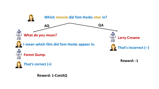
Figure 7.4: An illustration of the poor-student setting for RL Task 1 (Question Paraphrase).

7.2.2 Mechanical Turk Data

Finally, to validate our approach beyond our simulator by using real language, we collected data via Amazon Mechanical Turk. Due to the cost of data collection, we focused on real language versions of Tasks 4 (Knowledge Verification) and 8 (Missing Triple), see Secs. 7.1.2 and 7.1.3 for the simulator versions. That is, we collect dialogues and use them in an offline supervised learning setup similar to Section 7.2.1. This setup allows easily reproducible experiments.

For Mechanical Turk Task 4, the bot is asked a question by a human teacher, but before answering can ask the human if the question is related to one of the facts it knows about from its memory. It is then required to answer the original question, after some additional dialog turns relating to other question/answer pairs (called “conversational history”, as before). For Task 8, the bot is asked a question by a human but lacks the triple in its memory that would be needed to answer it. It is allowed to ask for the missing information, the human responds to the question in free-form language. The bot is then required to answer the original question, again after some “conversational history” has transpired.

We collect around 10,000 episodes (dialogues) for training, 1000 for validation, and 2500 for testing for each of the two tasks. In each case, we give instructions to the Turkers that still follow the original form of the task, but make the tasks contain realistic language written by humans.

For both tasks, while the human turkers replace the simulator that the bot was previously conversing with, the bot’s dialogue actions (capabilities) are essentially unchanged from before. That is, when answering questions, now the bot is required to answer a human’s questions rather than templated questions from the simulator. When the bot is asking questions, the bot still asks in the same form as before, e.g., questions like “Does it have something to do with X” for Task 4 or “I don’t know. What’s the answer?” for Task 8. However, now its questions are answered by a human. In both cases (asking and answering) the human data is richer with potentially more complex language and lexical variability. Examples of the collected dialogues are given in Figure 7.5.

MTurk Task 4: Knowledge Verification (AQ):

kb: In Their Skin written_by Joshua Close, Jeremy Power Regimbal

kb: In Their Skin starred_actors Selma Blair, James D’arcy, Rachel Miner, Joshua Close

T: What film was written by Joshua Close?

S: Does it have something to do with “In Their Skin starred_actors Joshua Close”?

T: No we were looking for who wrote the film not who starred in it.

…

MTurk Task 8: Missing Triple (AQ):

T :What movies does Timothy Scott Bogart have writing credit for?

S: I don’t know. What’s the answer?

T: Extreme Ops or The I Inside is the right answer.

…

Figure 7.5: Sample dialogues for Mechanical Turk versions of Tasks 4 and 8. Compared to the original tasks (see Figs 7.2 and 7.3) the teacher’s questions, and the teacher responses to the student’s questions, are written by humans and are more complex and contain more variety.

7.3 Models

For both offline supervised and online RL settings, we use the End-to-End Memory Network model (MemN2N) (Sukhbaatar et al., 2015) as a backbone. The model takes as input the last utterance of the dialogue history (the question from the teacher) as well as a set of memory contexts including short-term memories (the dialogue history between the bot and the teacher) and long-term memories (the knowledge base facts that the bot has access to), and outputs a label.

Offline Supervised Settings: The first learning strategy we adopt is the reward-based imitation strategy (denoted vanilla-MemN2N) described in Weston (2016), where at training time, the model maximizes the log likelihood probability of the correct answers the student gave (examples with incorrect final answers are discarded). Candidate answers are words that appear in the memories, which means the bot can only predict the entities that it has seen or known before.

We also use a variation of MemN2N called “context MemN2N” (Cont-MemN2N for short) where we replace each word’s embedding with the average of its embedding (random for unseen words) and the embeddings of the other words that appear around it. We use both the preceeding and following words as context and the number of context words is a hyperparameter selected on the dev set.

An issue with both vanilla-MemN2N and Cont-MemN2N is that the model only makes use of the bot’s answers as signals and ignores the teacher’s feedback. We thus propose to use a model that jointly predicts the bot’s answers and the teacher’s feedback (denoted as TrainQA (+FP)). The bot’s answers are predicted using a vanilla-MemN2N and the teacher’s feedback is predicted using the Forward Prediction (FP) model as described in Weston (2016). At training time, the models learn to jointly predict the teacher’s feedback and the answers with positive reward. At test time, the model will only predict the bot’s answer.

For the TestModelAQ setting described in Section 7.2, the model needs to decide the question to ask. Again, we use vanilla-MemN2N that takes as input the question and contexts, and outputs the question the bot will ask.

Online RL Settings: A binary vanilla-MemN2N (denoted as $P_{RL}(Question)$) is used to decide whether the bot should or should not ask a question, with the teacher replying if the bot does ask something. A second MemN2N is then used to decide the bot’s answer, denoted as $P_{RL}(Answer)$. $P_{RL}(Answer)$ for $QA$ and $AQ$ are two separate models, which means the bot will use different models for final-answer prediction depending on whether it chooses to ask a question or not.

We use the REINFORCE algorithm (Williams, 1992) to update $P_{RL}(Question)$ and $P_{RL}(Answer)$. For each dialogue, the bot takes two sequential actions $(a_{1},a_{2})$: to ask or not to ask a question (denoted as $a_{1}$); and guessing the final answer (denoted as $a_{2}$). Let $r(a_{1},a_{2})$ denote the cumulative reward for the dialogue episode, computed using Table 7.1. The gradient to update the policy is given by:

$$p(a_{1},a_{2})=P_{RL}(Question)(a_{1})\cdot P_{RL}(answer)(a_{2})$$ (7.1)

$$\nabla J(\theta)\approx\nabla\log p(a_{1},a_{2})[r(a_{1},a_{2})-b]$$

where $b$ is the baseline value, which is estimated using another MemN2N model that takes as input the query $x$ and memory $C$, and outputs a scalar $b$ denoting the estimation of the future reward. The baseline model is trained by minimizing the mean squared loss between the estimated reward $b$ and actual cumulative reward $r$, $||r-b||^{2}$. We refer the readers to Zaremba and Sutskever (2015) for more details. The baseline estimator model is independent from the policy models and the error is not backpropagated back to them.

In practice, we find the following training strategy yields better results: first train only $P_{RL}(answer)$, updating gradients only for the policy that predicts the final answer. After the bot’s final-answer policy is sufficiently learned, train both policies in parallel. This has a real-world analogy where the bot first learns the basics of the task, and then learns to improve its performance via a question-asking policy tailored to the user’s patience (represented by $cost_{AQ}$) and its own ability to asnwer questions.

7.4 Experiments

7.4.1 Offline Results

Offline results are presented in Tables 7.2, 7.3, and 7.4. Table 7.3 presents results for the vanilla-MemN2N and Forward Prediction models. Table 7.2 presents results for Cont-MemN2N, which is better at handling unknown words. We repeat each experiment 10 times and report the best result. Finally, Table 7.4 presents results for the test scenario where the bot itself chooses when to ask questions. Observations can be summarized as as follows:

	Question Clarification				Knowledge Operation
	Task 1: Q. Paraphrase		Task 2: Q. Verification		Task 3: Ask For Relevant K.		Task 4: K. Verification
Train \Test	TestQA	TestAQ	TestQA	TestAQ	TestQA	TestAQ	TestQA	TestAQ
TrainQA (Context)	0.754	0.726	0.742	0.684	0.883	0.947	0.888	0.959
TrainAQ (Context)	0.640	0.889	0.643	0.807	0.716	0.985	0.852	0.987
TrainMix (Context)	0.751	0.846	0.740	0.789	0.870	0.985	0.875	0.985

	Knowledge Acquisition
	Task 5: Q. Entity		Task 6: Answer Entity		Task 7: Relation Entity		Task 8: Triple		Task 9: Everything
Train \Test	TestQA	TestAQ	TestQA	TestAQ	TestQA	TestAQ	TestQA	TestAQ	TestQA	TestAQ
TrainQA (Context)	$<$0.01	0.224	$<$0.01	0.120	0.241	0.301	0.339	0.251	$<$0.01	0.058
TrainAQ (Context)	$<$0.01	0.639	$<$0.01	0.885	0.143	0.893	0.154	0.884	$<$0.01	0.908
TrainMix (Context)	$<$0.01	0.632	$<$0.01	0.852	0.216	0.898	0.298	0.886	$<$0.01	0.903

Table 7.2: Results for Cont-MemN2N on different tasks.

	Question Clarification				Knowledge Operation
	Task 1: Q. Paraphrase		Task 2: Q. Verification		Task 3: Ask For Relevant K.		Task 4: K. Verification
Train \Test	TestQA	TestAQ	TestQA	TestAQ	TestQA	TestAQ	TestQA	TestAQ
TrainQA	0.338	0.284	0.340	0.271	0.462	0.344	0.482	0.322
TrainAQ	0.213	0.450	0.225	0.373	0.187	0.632	0.283	0.540
TrainAQ(+FP)	0.288	0.464	0.146	0.320	0.342	0.631	0.311	0.524
TrainMix	0.326	0.373	0.329	0.326	0.442	0.558	0.476	0.491

	Knowledge Acquisition
	Task 5: Q. Entity		Task 6: Answer Entity		Task 7: Relation Entity		Task 8: Triple		Task 9: Everything
Train \Test	TestQA	TestAQ	TestQA	TestAQ	TestQA	TestAQ	TestQA	TestAQ	TestQA	TestAQ
TrainQA (vanila)	$<0.01$	0.223	$<$0.01	$<$0.01	0.109	0.129	0.201	0.259	$<$0.01	$<$0.01
TrainAQ (vanila)	$<0.01$	0.660	$<$0.01	$<$0.01	0.082	0.156	0.124	0.664	$<$0.01	$<$0.01
TrainAQ(+FP)	$<0.01$	0.742	$<0.01$	$<0.01$	0.085	0.188	0.064	0.702	$<$0.01	$<$0.01
Mix (vanila)	$<$0.01	0.630	$<$0.01	$<$0.01	0.070	0.152	0.180	0.572	$<$0.01	$<$0.01

Table 7.3: Results for offline settings using memory networks.

	Question Clarification	Knowledge Acquisition
	Task 2: Q. Verification	Task 4: K. Verification
	TestModelAQ	TestModelAQ
TrainAQ	0.382	0.480
TrainAQ(+FP)	0.344	0.501
TrainMix	0.352	0.469

Table 7.4: Results for TestModelAQ settings.

- Asking questions helps at test time, which is intuitive since it provides additional evidence:

• TrainAQ+TestAQ (questions can be asked at both training and test time) performs the best across all the settings.

• TrainQA+TestAQ (questions can be asked at training time but not at test time) performs worse than TrainQA+TestQA (questions can be asked at neither training nor test time) in tasks Question Clarification and Knowledge Operation due to the discrepancy between training and testing.

• TrainQA+TestAQ performs better than TrainQA+TestQA on all Knowledge Acquisition tasks, the only exception being the Cont-MemN2N model on the Missing Triple setting. The explanation is that for most tasks in Knowledge Acquisition, the learner has no chance of giving the correct answer without asking questions. The benefit from asking is thus large enough to compensate for the negative effect introduced by data discrepancy between training and test time.

• TrainMix offers flexibility in bridging the gap between datasets generated using QA and AQ, very slightly underperforming TrainAQ+TestAQ, but gives competitive results on both TestQA and TestAQ in the Question Clarification and Knowledge Operations tasks.

• TrainAQ+TestQA (allowing questions at training time but forbid questions at test time) performs the worst, even worse than TrainQA+TestQA. This has a real-world analogy where a student becomes dependent on the teacher answering their questions, later struggling to answer the test questions without help.

• In the Missing Question Entity task (the student does not know about the question entity), the Missing Answer Entity task (the student does not know about the answer entity), and Missing Everything task, the bot achieves accuracy less than 0.01 if not asking questions at test time (i.e., TestQA).

• The performance of TestModelAQ, where the bot relies on its model to ask questions at test time (and thus can ask irrelevant questions) performs similarly to asking the correct question at test time (TestAQ) and better than not asking questions (TestQA).

- Cont-MemN2N significantly outperforms vanilla-MemN2N. One explanation is that considering context provides significant evidence distinguishing correct answers from candidates in the dialogue history, especially in cases where the model encounters unfamiliar words.

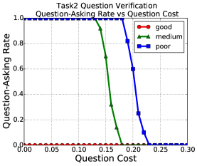
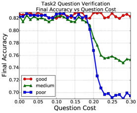
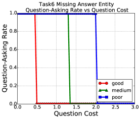
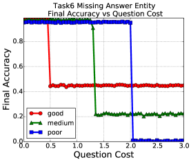
Figure 7.6: Results of online learning for Task 2 and Task 6

7.4.2 RL Results

For the RL settings, we present results for Task 2 (Question Verification) and Task 6 (Missing Answer Entities) in Figure 7.6. Task 2 represents scenarios where different types of student have different abilities to correctly answer questions (e.g., a poor student can still sometimes give correct answers even when they do not fully understand the question). Task 6 represents tasks where a poor learner who lacks the knowledge necessary to answer the question can hardly give a correct answer. All types of students including the good student will theoretically benefit from asking questions (asking for the correct answer) in Task 6. We show the percentage of question-asking versus the cost of AQ on the test set and the accuracy of question-answering on the test set vs the cost of AQ. Our main findings were:

• A good student does not need to ask questions in Task 2 (Question Verification), because they already understand the question. The student will raise questions asking for the correct answer when cost is low for Task 6 (Missing Answer Entities).

• A poor student always asks questions when the cost is low. As the cost increases, the frequency of question-asking declines.

• As the AQ cost increases gradually, good students will stop asking questions earlier than the medium and poor students. The explanation is intuitive: poor students benefit more from asking questions than good students, so they continue asking even with higher penalties.

• As the probability of question-asking declines, the accuracy for poor and medium students drops. Good students are more resilient to not asking questions.

7.4.3 Mechanical Turk Results

	vanilla-MemN2N				Cont-MemN2N
	Task 4: K. Verification		Task 8: Triple		Task 4: K. Verification		Task 8: Triple
Train \Test	TestQA	TestAQ	TestQA	TestAQ	TestQA	TestAQ	TestQA	TestAQ
TrainQA	0.331	0.313	0.133	0.162	0.712	0.703	0.308	0.234
TrainAQ	0.318	0.375	0.072	0.422	0.679	0.774	0.137	0.797

Table 7.5: Mechanical Turk Task Results. Asking Questions (AQ) outperforms only answering questions without asking (QA).

	vanilla-MemN2N				Cont-MemN2N
	Task 4: K. Verification		Task 8: Triple		Task 4: K. Verification		Task 8: Triple
Train \Test	TestQA	TestAQ	TestQA	TestAQ	TestQA	TestAQ	TestQA	TestAQ
TrainQA	0.331	0.313	0.133	0.162	0.712	0.703	0.308	0.234
TrainAQ	0.318	0.375	0.072	0.422	0.679	0.774	0.137	0.797

Table 7.6: Mechanical Turk Task Results, using real data for training and testing.

	vanilla-MemN2N				Cont-MemN2N
	Task 4: K. Verification		Task 8: Triple		Task 4: K. Verification		Task 8: Triple
Train \Test	TestQA	TestAQ	TestQA	TestAQ	TestQA	TestAQ	TestQA	TestAQ
TrainQA	0.356	0.311	0.128	0.174	0.733	0.717	0.368	0.352
TrainAQ	0.340	0.445	0.150	0.487	0.704	0.792	0.251	0.825

Table 7.7: Results on Mechanical Turk Tasks using a combination of real and simulated data for training, testing on real data.

	vanilla-MemN2N				Cont-MemN2N
	Task 4: K. Verification		Task 8: Triple		Task 4: K. Verification		Task 8: Triple
Train \Test	TestQA	TestAQ	TestQA	TestAQ	TestQA	TestAQ	TestQA	TestAQ
TrainQA	0.340	0.311	0.120	0.165	0.665	0.648	0.349	0.342
TrainAQ	0.326	0.390	0.067	0.405	0.642	0.714	0.197	0.788

Table 7.8: Results on Mechanical Turk Tasks using only simulated data for training, but testing on real data.

Results for the Mechanical Turk Tasks are given in Table 7.5. We again compare vanilla-MemN2N and Cont-MemN2N, using the same TrainAQ/TrainQA and TestAQ/TestQA combinations as before, for Tasks 4 and 8 as described in Section 7.2.2. We tune hyperparameters on the validation set and repeat each experiment 10 times and report the best result.

While performance is lower than on the related Task 4 and Task 8 simulator tasks, we still arrive at the same trends and conclusions when real data from humans is used. The performance was expected to be lower because (i) real data has more lexical variety, complexity, and noise; and (ii) the training set was smaller due to data collection costs (10k vs. 180k).

More importantly, the same main conclusion is observed as before: TrainAQ+TestAQ (questions can be asked at both training and test time) performs the best across all the settings. That is, we show that a bot asking questions to humans learns to outperform one that only answers them.

We also provide additional experiments. In Table 7.5, results were shown when training and testing on the collected Mechanical Turk data (around 10,000 episodes of training dialogues for training). As we collected the data in the same settings as Task 4 and 8 of our simulator, we could also consider supplementing training with simulated data as well, of which we have a larger amount (over 100,000 episodes). Note this is only for training, we will still test on the real (Mechanical Turk collected) data. Although the simulated data has less lexical variety as it is built from templates, the larger size might obtain improve results.

Results are given in Table 7.8 when training on the combination of real and simulator data, and testing on real data. This should be compared to training on only the real data (Table 7.8) and only on the simulator data (Table 7.8). The best results are obtained from the combination of simulator and real data. The best real data only results (selecting over algorithm and training strategy) on both tasks outperform the best results using simulator data, i.e. using Cont-MemN2N with the Train AQ / TestAQ setting) 0.774 and 0.797 is obtained vs. 0.714 and 0.788 for Tasks 4 and 8 respectively. This is despite there being far fewer examples of real data compared to simulator data. Overall we obtain two main conclusions from this additional experiment: (i) real data is indeed measurably superior to simulated data for training our models; (ii) in all cases (across different algorithms, tasks, and data types – be they real data, simulated data or combinations) the bot asking questions (AQ) outperforms it only answering questions and not asking them (QA). The latter reinforces the main result of the paper.

Chapter 8 Dialogue Learning with Human-in-the-Loop

In this chapter, we will discuss how a bot can improve in an online fashion from humans’ feedback. A good conversational agent should have the ability to learn from the online feedback from a teacher: adapting its model when making mistakes and reinforcing the model when the teacher’s feedback is positive. This is particularly important in the situation where the bot is initially trained in a supervised way on a fixed synthetic, domain-specific or pre-built dataset before release, but will be exposed to a different environment after release (e.g., more diverse natural language utterance usage when talking with real humans, different distributions, special cases, etc.). Most recent research has focused on training a bot from fixed training sets of labeled data but seldom on how the bot can improve through online interaction with humans. Human (rather than machine) language learning happens during communication (Bassiri, 2011; Werts et al., 1995), and not from labeled datasets, hence making this an important subject to study.

In this chapter, we explore this direction by training a bot through interaction with teachers in an online fashion. The task is formalized under the general framework of reinforcement learning via the teacher’s (dialogue partner’s) feedback to the dialogue actions from the bot. The dialogue takes place in the context of question-answering tasks and the bot has to, given either a short story or a set of facts, answer a set of questions from the teacher. We consider two types of feedback: explicit numerical rewards as in conventional reinforcement learning, and textual feedback which is more natural in human dialogue. We consider two online training scenarios: (i) where the task is built with a dialogue simulator allowing for easy analysis and repeatability of experiments; and (ii) where the teachers are real humans using Amazon Mechanical Turk.

We explore important issues involved in online learning such as how a bot can be most efficiently trained using a minimal amount of teacher’s feedback, how a bot can harness different types of feedback signal, how to avoid pitfalls such as instability during online learing with different types of feedback via data balancing and exploration, and how to make learning with real humans feasible via data batching. Our findings indicate that it is feasible to build a pipeline that starts from a model trained with fixed data and then learns from interactions with humans to improve itself.

8.1 Dataset and Tasks

We begin by describing the data setup we use. In our first set of experiments we build a simulator as a testbed for learning algorithms. In our second set of experiments we use Mechanical Turk to provide real human teachers giving feedback.

8.1.1 Simulator

The simulator adapts two existing fixed datasets to our online setting. Following Weston (2016), we use (i) the single supporting fact problem from the bAbI datasets Weston et al. (2016) which consists of 1000 short stories from a simulated world interspersed with questions; and (ii) the WikiMovies dataset Weston et al. (2016) which consists of roughly 100k (templated) questions over 75k entities based on questions with answers in the open movie database (OMDb). Each dialogue takes place between a teacher, scripted by the simulation, and a bot. The communication protocol is as follows: (1) the teacher first asks a question from the fixed set of questions existing in the dataset, (2) the bot answers the question, and finally (3) the teacher gives feedback on the bot’s answer.

Tasks

We follow the paradigm defined in Weston (2016) where the teacher’s feedback takes the form of either textual feedback, a numerical reward, or both, depending on the task. For each dataset, there are ten tasks:

• Task 1: The teacher tells the student exactly what they should have said (supervised baseline).

• Task 2: The teacher replies with positive textual feedback and reward, or negative textual feedback.

• Task 3: The teacher gives textual feedback containing the answer when the bot is wrong.

• Task 4: The teacher provides a hint by providing the class of the correct answer, e.g., “No it’s a movie” for the question “which movie did Forest Gump star in?”.

• Task 5: The teacher provides a reason why the student’s answer is wrong by pointing out the relevant supporting fact from the knowledge base.

• Task 6: The teacher gives positive reward only 50% of the time.

• Task 7: Rewards are missing and the teacher only gives natural language feedback.

• Task 8: Combines Tasks 1 and 2 to see whether a learner can learn successfully from both forms of supervision at once.

• Task 9: The bot asks questions of the teacher about what it has done wrong.

• Task 10: The bot will receive a hint rather than the correct answer after asking for help.

T : Which movie did Tom Hanks star in ?		T : Which movie did Tom Hanks star in ?
S : Forrest Gump		S : Brad Pitt.
Task 1: Imitating an Expert Student		Task 1: Imitating an Expert Student
S: Forrest Gump		S: Forrest Gump
T: (no response)		T: (no response)
Task 2: Positive and Negative Feedback		Task 2: Positive and Negative Feedback
T: Yes, that’s right! (+)		T: No, that’s incorrect!
Task 3: Answers Supplied by Teacher		Task 3: Answers Supplied by Teacher
T: Yes, that is correct. (+)		T: No, the answer is Forrest Gump !
Task 4: Hints Supplied by Teacher		Task 4: Hints Supplied by Teacher
T: Correct! (+)		T: No, it’s a movie !
Task 5: Supporting Facts Supplied by Teacher		Task 5: Supporting Facts Supplied by Teacher
T: That’s right. (+)		T: No, because Forrest Gump starred actors
		Tom Hanks, Robin Wright, Gary Sinise !
Task 6: Partial Feedback		Task 6: Partial Feedback
if random(0,1)$<$0.5 then		T: Sorry, wrong.
T: That’s correct. (+)
else  T: That’s correct.
Task 7: No Feedback		Task 7: No Feedback
T: Yes.		T: No.
Task 8: Imitation and Feedback Mixture		Task 8: Imitation and Feedback Mixture
if random(0,1)$<$0.5 then		if random(0,1)$<$0.5 then
T: Yes, that’s right! (+)		T: Wrong.
else  T: (no response)		else   S: Forrest Gump
Task 9: Asking For Corrections		Task 9: Asking For Corrections
T: Correct! (+)		T: No, that’s wrong.
		S: Can you help me?
		T: Forrest Gump !
Task 10: Asking For Supporting Facts		Task 10: Asking For Supporting Facts
T: Yes, that’s right! (+)		T: Sorry, that’s not it.
		S: Can you help me?
		T: A relevant fact is that Forrest Gump starred actors
		Tom Hanks, Robin Wright, Gary Sinise !

Figure 8.1: The ten tasks our simulator implements, which evaluate different forms of teacher response and binary feedback. In each case the same example from WikiMovies is given for simplicity, where the student answered correctly for all tasks (left) or incorrectly (right). Red text denotes responses by the bot with S denoting the bot. Blue text is spoken by the teacher with T denoting the teacher’s response. For imitation learning the teacher provides the response the student should say denoted with S in Tasks 1 and 8. A (+) denotes a positive reward.

Here, we only consider Task 6 (“partial feedback”): the teacher replies with positive textual feedback (6 possible templates) when the bot answers correctly, and positive reward is given only 50% of the time. When the bot is wrong, the teacher gives textual feedback containing the answer. Example dialogues are given in Figure 8.2.

bAbI Task 6: Partial Rewards		WikiMovies Task 6: Partial Rewards
Mary went to the hallway.		What films are about Hawaii?                       50 First Dates
John moved to the bathroom.		Correct!
Mary travelled to the kitchen.		Who acted in Licence to Kill?                       Billy Madison
Where is Mary?                         kitchen		No, the answer is Timothy Dalton.
Yes, that’s right!		What genre is Saratoga Trunk in?                       Drama
Where is John?                          bathroom		Yes! (+)
Yes, that’s correct! (+)		…

Figure 8.2: Simulator sample dialogues for the bAbI task (left) and WikiMovies (right). We consider 10 different tasks following Weston (2016). The teacher’s dialogue is in black and the bot is in red. ${{\color[rgb]{0,0,1}(+)}}$ indicates receiving positive reward, given only 50% of the time even when correct.

Sample dialogues with correct answers from the bot:

Who wrote the Linguini Incident ?                                           richard shepard

Richard Shepard is one of the right answers here.

What year did The World Before Her premiere?                       2012

Yep! That’s when it came out.

Which are the movie genres of Mystery of the 13th Guest?     crime

Right, it can also be categorized as a mystery.

Sample dialogues with incorrect answers from the bot:

What are some movies about a supermarket ?                           supermarket

There were many options and this one was not among them.

Which are the genres of the film Juwanna Mann ?                     kevin pollak

That is incorrect. Remember the question asked for a genre not name.

Who wrote the story of movie Coraline ?                                   fantasy

That’s a movie genre and not the name of the writer. A better answer would of been Henry Selick

or Neil Gaiman.

Figure 8.3: Human Dialogue from Mechanical Turk (based on WikiMovies) The human teacher’s dialogue is in black and the bot is in red. We show examples where the bot answers correctly (left) and incorrectly (right). Real humans provide more variability of language in both questions and textual feedback than in the simulator setup (cf. Figure 8.2).

  Title: Write brief responses to given dialogue exchanges (about 15 min)

Description: Write a brief response to a student’s answer to a teacher’s question, providing feedback to the student on their answer.

Instructions:

Each task consists of the following triplets:

1. a question by the teacher

2. the correct answer(s) to the question (separated by “OR”)

3. a proposed answer in reply to the question from the student

Consider the scenario where you are the teacher and have already asked the question, and received the reply from the student. Please compose a brief response giving feedback to the student about their answer. The correct answers are provided so that you know whether the student was correct or not.

For example, given 1) question: “what is a color in the united states flag?”; 2) correct answer: “white, blue, red”; 3) student reply: “red”, your response could be something like “that’s right!”; for 3) reply: “green”, you might say “no that’s not right” or “nope, a correct answer is actually white”.

Please vary responses and try to minimize spelling mistakes. If the same responses are copied/pasted or overused, we’ll reject the HIT.

Avoid naming the student or addressing “the class” directly.

We will consider bonuses for higher quality responses during review.
 

Figure 8.4: Instructions Given to Turkers

8.1.2 Mechanical Turk Experiments

We also extended WikiMovies using Mechanical Turk so that real human teachers are giving feedback rather than using a simulation. As both the questions and feedback are templated in the simulation, they are now both replaced with natural human utterances. Rather than having a set of simulated tasks, we have only one task, and we gave instructions to the teachers that they could give feedback as they see fit. The exact instructions given to the Turkers is given in Figure 8.4. In general, each independent response contains feedback like (i) positive or negative sentences; or (ii) a phrase containing the answer or (iii) a hint, which are similar to setups defined in the simulator. However, some human responses cannot be so easily categorized, and the lexical variability is much larger in human responses. Such a process also reflects the basic idea of curriculum learning Bengio et al. (2009), in which the model follows a specific curriculum, in which the model first learns from easy examples from the simulator and then from real dialogue interactions, which tend to be harder. Some examples of the collected data are given in Figure 8.3.

8.2 Methods

8.2.1 Reinforcement Learning

In this section, we present the algorithms we used to train MemN2N in an online fashion. Our learning setup can be cast as a particular form of Reinforcement Learning. The policy is implemented by the MemN2N model. The state is the dialogue history. The action space corresponds to the set of answers the MemN2N has to choose from to answer the teacher’s question. In our setting, the policy chooses only one action for each episode. The reward is either $1$ (a reward from the teacher when the bot answers correctly) or $0$ otherwise. Note that in our experiments, a reward equal to $0$ might mean that the answer is incorrect or that the positive reward is simply missing. The overall setup is closest to standard contextual bandits, except that the reward is binary.

When working with real human dialogues, e.g., collecting data via Mechanical Turk, it is easier to set up a task whereby a bot is deployed to respond to a large batch of utterances, as opposed to a single one. The latter would be more difficult to manage and scale up since it would require some form of synchronization between the model replicas interacting with each human.

This is comparable to the real world situation where a teacher can either ask a student a single question and give feedback right away, or set up a test that contains many questions and grade all of them at once. Only after the learner completes all questions, it can hear feedback from the teacher.

We use batch size to refer to how many dialogue episodes the current model is used to collect feedback before updating its parameters. In the Reinforcement Learning literature, batch size is related to off-policy learning since the MemN2N policy is trained using episodes collected with a stale version of the model. Our experiments show that our model and base algorithms are very robust to the choice of batch size, alleviating the need for correction terms in the learning algorithm (Bottou et al., 2013).

We consider two strategies: (i) online batch size, whereby the target policy is updated after doing a single pass over each batch (a batch size of 1 reverts to the usual on-policy online learning); and (ii) dataset-sized batch, whereby training is continued to convergence on the batch which is the size of the dataset, and then the target policy is updated with the new model, and a new batch is drawn and the procedure iterates. These strategies can be applied to all the methods we use, described below.

Next, we discuss the learning algorithms we considered in this work.

Reward-Based Imitation (RBI)

The simplest algorithm we first consider is the one employed in Weston (2016). RBI relies on positive rewards provided by the teacher. It is trained to imitate the correct behavior of the learner, i.e., learning to predict the correct answers (with reward 1) at training time and disregarding the other ones. This is implemented by using a MemN2N that maps a dialogue input to a prediction, i.e. using the cross entropy criterion on the positively rewarded subset of the data.

In order to make this work in the online setting which requires exploration to find the correct answer, we employ an $\epsilon$-greedy strategy: the learner makes a prediction using its own model (the answer assigned the highest probability) with probability $1-\epsilon$, otherwise it picks a random answer with probability $\epsilon$. The teacher will then give a reward of $+1$ if the answer is correct, otherwise $0$. The bot will then learn to imitate the correct answers: predicting the correct answers while ignoring the incorrect ones.

REINFORCE

The second algorithm we use is the REINFORCE algorithm (Williams, 1992), which maximizes the expected cumulative reward of the episode, in our case the expected reward provided by the teacher. The expectation is approximated by sampling an answer from the model distribution. Let $a$ denote the answer that the learner gives, $p(a)$ denote the probability that current model assigns to $a$, $r$ denote the teacher’s reward, and $J(\theta)$ denote the expectation of the reward. We have:

$$\nabla J(\theta)\approx\nabla\log p(a)[r-b]$$ (8.1)

where $b$ is the baseline value, which is estimated using a linear regression model that takes as input the output of the memory network after the last hop, and outputs a scalar $b$ denoting the estimation of the future reward. The baseline model is trained by minimizing the mean squared loss between the estimated reward $b$ and actual reward $r$, $||r-b||^{2}$. We refer the readers to Zaremba and Sutskever (2015) for more details. The baseline estimator model is independent from the policy model, and its error is not backpropagated through the policy model.

The major difference between RBI and REINFORCE is that (i) the learner only tries to imitate correct behavior in RBI while in REINFORCE it also leverages the incorrect behavior, and (ii) the learner explores using an $\epsilon$-greedy strategy in RBI while in REINFORCE it uses the distribution over actions produced by the model itself.

Forward Prediction (FP)

FP (Weston, 2016) handles the situation where a numerical reward for a bot’s answer is not available, meaning that there are no +1 or 0 labels available after a student’s utterance. Instead, the model assumes the teacher gives textual feedback $t$ to the bot’s answer, taking the form of a dialogue utterance, and the model tries to predict this instead. Suppose that $x$ denotes the teacher’s question and $C$=$c_{1}$, $c_{2}$, …, $c_{N}$ denotes the dialogue history as before. In FP, the model first maps the teacher’s initial question $x$ and dialogue history $C$ to a vector representation $u$ using a memory network with multiple hops. Then the model will perform another hop of attention over all possible student’s answers in $\mathbb{A}$, with an additional part that incorporates the information of which candidate (i.e., $a$) was actually selected in the dialogue:

$$p_{\hat{a}}=\operatorname{softmax}(u^{T}y_{\hat{a}})~{}~{}~{}~{}~{}o=\sum_{\hat{a}\in\mathbb{A}}p_{\hat{a}}(y_{\hat{a}}+\beta\cdot{\bf 1}[\hat{a}=a])$$ (8.2)

where $y_{\hat{a}}$ denotes the vector representation for the student’s answer candidate $\hat{a}$. $\beta$ is a (learned) d-dimensional vector to signify the actual action $a$ that the student chooses. $o$ is then combined with $u$ to predict the teacher’s feedback $t$ using a softmax:

$$u_{1}=o+u~{}~{}~{}~{}t=\operatorname{softmax}(u_{1}^{T}x_{r_{1}},u_{1}^{T}x_{r_{2}},...,u_{1}^{T}x_{r_{N}})$$ (8.3)

where $x_{r_{i}}$ denotes the embedding for the $i^{th}$ response. In the online setting, the teacher will give textual feedback, and the learner needs to update its model using the feedback. It was shown in Weston (2016) that in an off-line setting this procedure can work either on its own, or in conjunction with a method that uses numerical rewards as well for improved performance. In the online setting, we consider two simple extensions:

• $\epsilon$-greedy exploration: with probability $\epsilon$ the student will give a random answer, and with probability $1-\epsilon$ it will give the answer that its model assigns the largest probability. This method enables the model to explore the space of actions and to potentially discover correct answers.

• data balancing: cluster the set of teacher responses $t$ and then balance training across the clusters equally. This is a type of experience replay (Mnih et al., 2013) but sampling with an evened distribution. Balancing stops part of the distribution dominating the learning. For example, if the model is not exposed to sufficient positive and negative feedback, and one class overly dominates, the learning process degenerates to a model that always predicts the same output regardless of its input.

8.3 Experiments

Experiments are first conducted using our simulator, and then using Amazon Mechanical Turk with real human subjects taking the role of the teacher.

8.3.1 Simulator

Online Experiments

In our first experiments, we considered both the bAbI and WikiMovies tasks and varied batch size, random exploration rate $\epsilon$, and type of model. Figure 8.5 and Figure 8.6 shows (Task 6) results on bAbI and WikiMovies.

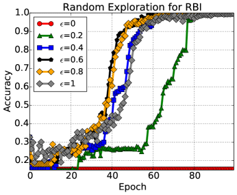
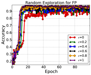
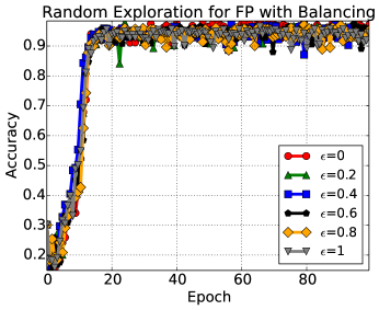
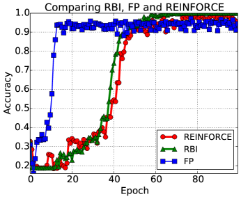
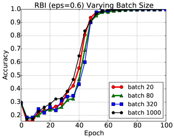
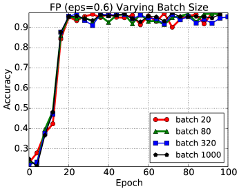
Figure 8.5: Training epoch vs. test accuracy for bAbI (Task 6) varying exploration $\epsilon$ and batch size. Random exploration is important for both reward-based (RBI) and forward prediction (FP). Performance is largely independent of batch size, and RBI performs similarly to REINFORCE. Note that supervised, rather than reinforcement learning, with gold standard labels achieves 100% accuracy on this task.

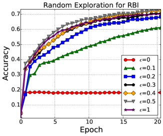
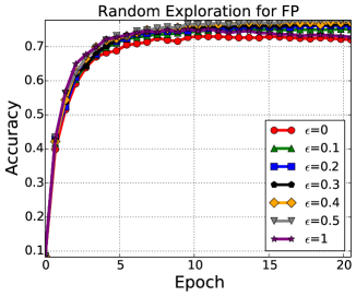
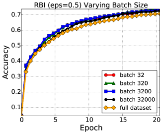
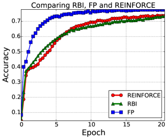
Figure 8.6: WikiMovies: Training epoch vs. test accuracy on Task $6$ varying (top left panel) exploration rate $\epsilon$ while setting batch size to $32$ for RBI, (top right panel) for FP, (bottom left) batch size for RBI, and (bottom right) comparing RBI, REINFORCE, and FP with $\epsilon=0.5$. The model is robust to the choice of batch size. RBI and REINFORCE perform comparably. Note that supervised, rather than reinforcement learning, with gold standard labels achieves 80% accuracy on this task (Weston, 2016).

Overall, we obtain the following conclusions:

• In general RBI and FP do work in a reinforcement learning setting, but can perform better with random exploration.

• In particular RBI can fail without exploration. RBI needs random noise for exploring labels otherwise it can get stuck predicting a subset of labels and fail.

• REINFORCE does not perform competitively. It obtains similar performance to RBI with optimal $\epsilon$.

• FP with balancing or with exploration via $\epsilon$ both outperform FP alone.

• For both RBI and FP, performance is largely independent of online batch size.

Dataset Batch Size Experiments

Given that larger online batch sizes appear to work well, and that this could be important in a real-world data collection setup where the same model is deployed to gather a large amount of feedback from humans, we conducted further experiments where the batch size is exactly equal to the dataset size and for each batch training is completed to convergence. After the model has been trained on the dataset, it is deployed to collect a new dataset of questions and answers, and the process is repeated. Table 8.1 reports test error at each iteration of training, using the bAbI Task $6$ as the case study. The following conclusions can be made for this setting:

• RBI improves in performance as we iterate. Unlike in the online case, RBI does not need random exploration. We believe this is because the first batch, which is collected with a randomly initialized model, contains enough variety of examples with positive rewards that the model does not get stuck predicting a subset of labels.

• FP is not stable in this setting. This is because once the model gets very good at making predictions (at the third iteration), it is not exposed to a sufficient number of negative responses anymore. From that point on, learning degenerates and performance drops as the model always predicts the same responses. At the next iteration, it will recover again since it has a more balanced training set, but then it will collapse again in an oscillating behavior.

• FP does work if extended with balancing or random exploration with sufficiently large $\epsilon$.

• RBI+FP also works well and helps with the instability of FP, alleviating the need for random exploration and data balancing.

Overall, our simulation results indicate that while a bot can be effectively trained fully online from bot-teacher interactions, collecting real dialogue data in batches (which is easier to collect and iterate experiments over) is also a viable approach. We hence pursue the latter approach in our next set of experiments.

Iteration	1	2	3	4	5	6
Imitation Learning	0.24	0.23	0.23	0.22	0.23	0.23
Reward Based Imitation (RBI)	0.74	0.87	0.90	0.96	0.96	0.98
Forward Pred. (FP)	0.99	0.96	1.00	0.30	1.00	0.29
RBI+FP	0.99	0.96	0.97	0.95	0.94	0.97
FP (balanced)	0.99	0.97	0.97	0.97	0.97	0.97
FP (rand. exploration $\epsilon=0.25$)	0.96	0.88	0.94	0.26	0.64	0.99
FP (rand. exploration $\epsilon=0.5$)	0.98	0.98	0.99	0.98	0.95	0.99

Table 8.1: Test accuracy of various models per iteration in the dataset batch size case (using batch size equal to the size of the full training set) for bAbI, Task $6$. Results $>0.95$ are in bold.

8.3.2 Human Feedback

We employed Turkers to both ask questions and then give textual feedback on the bot’s answers, as described in Section 8.1.2. Our experimental protocol was as follows. We first trained a MemN2N using supervised (i.e., imitation) learning on a training set of 1000 questions produced by Turkers and using the known correct answers provided by the original dataset (and no textual feedback). Next, using the trained policy, we collected textual feedback for the responses of the bot for an additional 10,000 questions. Examples from the collected dataset are given in Figure 8.3. Given this dataset, we compare various models: RBI, FP, and FP+RBI. As we know the correct answers to the additional questions, we can assign a positive reward to questions the bot got correct. We hence measure the impact of the sparseness of this reward signal, where a fraction $r$ of additional examples have rewards. The models are tested on a test set of $\sim$8,000 questions (produced by Turkers), and hyperparameters are tuned on a similarly sized validation set. Note this is a harder task than the WikiMovies task in the simulator due to the use natural language from Turkers, hence lower test performance is expected.

Results are given in Table 8.2. They indicate that both RBI and FP are useful. When rewards are sparse, FP still works via the textual feedback while RBI can only use the initial 1000 examples when $r=0$. As FP does not use numericalrewards at all, it is invariant to the parameter $r$. The combination of FP and RBI outperforms either alone.

Model	$r=0$	$r=0.1$	$r=0.5$	$r=1$
Reward Based Imitation (RBI)	0.333	0.340	0.365	0.375
Forward Prediction (FP)	0.358	0.358	0.358	0.358
RBI+FP	0.431	0.438	0.443	0.441

Table 8.2: Textual feedback is provided for 10,000 model predictions (from a model trained with 1k labeled training examples), and additional sparse binary rewards (fraction $r$ of examples have rewards). Forward Prediction and Reward-based Imitation are both useful, with their combination performing best.

8.4 Conclusion

We studied dialogue learning of end-to-end models using textual feedback and numerical rewards. Both fully online and iterative batch settings are viable approaches to policy learning, as long as possible instabilities in the learning algorithms are taken into account. Secondly, we showed for the first time that the FP method can work in both an online setting and on real human feedback. Overall, our results indicate that it is feasible to build a practical pipeline that starts with a model trained on an initial fixed dataset, which then learns from interactions with humans in a (semi-)online fashion to improve itself.

For the results, we can see that there is still a gap between the model only trained based on the simulator and the one bootstrapped from human feedback. This suggests that further improvement could be achieved when more human-in-the-loop efforts are incorporated.

Chapter 9 Conclusion and Future Work

In this dissertation, we have presented methods for developing more human-like and interactive conversational agents. We discussed the opportunities presented by current deep-learning models in chat-bot development, along with challenges that arise, and how to tackle them. In this section, we will conclude this thesis and discuss the challenges that are still faced by current conversational systems, and suggest future work to tackle them.

In Chapter 3, we discussed how to address the issue that current neural chit-chat systems tend to produce dull, generic, and uninteresting responses such as “i don’t know” or “i don’t know what you are talking about. We discovered that this is due to the maximum-likelihood objective function adopted in standard sequence generation systems. We proposed using mutual information as the objective function in place of the MLE objective function, where we not only want the generated response to be specific to the input dialogue history, but want the dialogue history to be specific to the generated response as well. Using MMI as an objective function, we observed that the model is able to generate more specific, coherent, and interesting responses.

In Chapter 4, we discussed how to give the model a consistent persona to preserve its speaker consistency. We proposed using user embeddings to encode the information of users, such as user attributes or word usage tendency. These embeddings are incorporated into the neural encoder-decoder models, pushing the model to generate more consistent responses. We also proposed a speaker-addressee model, in which the utterance that the conversational agent generates not only depends on the identify of the speaker, but also the identify of its dialogue parter. We observe a clear performance improvement introduced by the proposed persona model and the speaker-addressee model in automatic evaluation metrics BLEU and perplexity. Human evaluation performed by Turkers also demonstrates that the proposed persona model is able to generate more consistent responses than the vanilla Seq2Seq models.

In Chapter 5, we proposed a multi-turn dialogue system, in which we are not only concerned with the quality of single-turn conversations, but the overall success of multi-turn conversations. The MLE objective function used in standard Seq2Seq models is trained to predict the next turn utterance, and is thus not suited for a system optimized for multi-turn dialogue success, especially because the positive or negative outcome of a dialogue utterance in a multi-turn dialogue usually does not show up after a few turns later. We proposed to tackle this issue using reinforcement learning, in which we created a scenario for the two bots to talk with each other. We manually designed three types of rewards that we think are important for a successful conversation, namely, ease to follow, informational flow, and meaningfulness. The RL system is trained to push the system to generate responses that are highly rewarded regarding these three aspects. Human evaluation illustrates that the proposed RL system tends to generate more sustainable conversations.

In Chapter 6, we proposed a more generic reward function for training a RL-based dialogue system: a machine-generated response is highly rewarded it it is indistinguishable human-generated responses. We proposed using adversarial learning, in which we jointly train two models, a generator that defines the probability of generating a dialogue sequence given input dialogue history, and a discriminator that labels dialogues as human-generated or machine-generated. We cast the task as a reinforcement learning problem, in which the quality of machine-generated utterances is measured by its ability to fool the discriminator into believing that it is a human-generated one. The output from the discriminator is used as a reward to the generator, pushing it to generate utterances indistinguishable from human-generated dialogues. Human evaluation reveals that that the proposed adversarial reinforcement learning is able to generate better-quality responses.

In Chapter 7, we focused on the task of developing interactive QA dialogue agents, where we give an agent the ability to ask its dialogue partner questions. We define three scenarios where we think the bot can benefit from asking questions: (1) question clarification, in which the bot asks its dialogue partner for text clarification; (2) knowledge operation, in which the bot asks the teacher for hints on relevant knowledge-base fact; and (3) knowledge acquisition, in which the bot asks about new knowledge. We validated that the bot always benefits from asking questions in these three scenarios. We additionally explored how a bot can learn when it should ask questions by designing a setting where the action of question asking comes at a cost. This has real-world implications since it would be user-unfriendly if a dialogue agent asks questions all the time. We designed a reinforcement learning system, within which the bot is able to automatically figure out when it should ask questions that will lead to highest future rewards.

In Chapter 8, we designed a RL system that gives the bot the ability to learn from online feedback: adapting its model when making mistakes and reinforcing the model when users’ feedback is positive. The bot takes advantage of both explicit numerical rewards, and textual feedback which is more natural in human dialogue. We explore important issues such as how a bot can be most efficiently trained using a minimal amount of user feedback, how to avoid pitfalls such as instability during online learning with different types of feedback via data balancing and exploration, and how to make learning with real humans feasible via data batching. We show that it is feasible to build a pipeline that starts from a model trained with fixed data and then learns from interactions with humans to improve itself.

Together, these contributions have created a system that is able to generate more interactive, smart, user-consistent, long-term successful chit-chat system.  
 
We will conclude this dissertation with a discussion of the challenges that current chit-chat systems still face, and suggest some avenues for future research.

Context

In this thesis, we use a hierarchical LSTM models with attention to capture contexts, where a word-level of LSTM is used to obtain the representation for each context sentence, and another level LSTM combines sentence-level representations into a context vector to represent the entire dialogue history. But it is not straightforwardly clear how much context information this context vector is able to capture, and how well this hierarchical attention model is able to separate informational wheat from chaff. This incapability might stem from (1) the lack of capacity of current neural network models, where one single context information doesn’t have enough capacity to encode all context information or (2) the model’s incapability of figuring out which context sentence provides more evidence than others on what the bot should say next. Tackling these issues is extremely important in real-world applications such as customer service chatbot development. Think about the domain of mailing package tracking, in which the bot needs to memorize some important information such as a tracking number throughout the conversation. Combining information extraction methods or a slot filling strategy that extracts important entities in the dialogue history with representation-based neural models has the potential to tackle this problem. Intuitively, only a very small fraction of key words in the dialogue history have significant guidance on what the bot should talk about. Using a key-word based information extraction model that first extracts these keywords and then incorporates them into the context neural model provides more flexibility in leveraging information from larger history context.

Furthermore, textual context only consists one specific type of evidence when we humans converse. Our conversations are also grounded on visual context, e.g., what we see and the environment (e.g., in a car) in which the conversation takes place. Being able to leveraging visual information (and also other types of information) will significantly narrow down the topics to discuss, and will consequentially lead to responses of better quality.

Logics and Pragmatics

Think about the following two contexts of an ongoing conversation: A: are you going to the party? B: Sorry, I have an exam tomorrow. From this context, we know that the speaker $B$ is not going to the party because he has to prepare for the upcoming exam, on which the conversation that follows should be based. This requires a sequence of reasoning steps, namely, having an exam tomorrow $\rightarrow$ having to prepare for the exam $\rightarrow$ being occupied $\rightarrow$ not able to attend the party. Straightforward as it seems to humans, such a line of reasoning is extremely hard for current machine learning systems, especially in an open-domain: manually labeling all the reasoning chains in an open domain is unrealistically work-demaning. We thus need a logic deduction model, which automatically learns these implicit reasoning chains from a massive amount of training data and then incorporate them to conversational generation.

Background and Prior Knowledge

Human conversations always take place in a specific context or background. The granularity could be as small/specific as the location that a conversation takes place in (e.g., a cafeteria or a theater), or as large as during war time vs peaceful time. This background has a significant impact on how the conversation should go. The context also includes user information, personal attributes, or even the speaker’s general feeling for his dialogue partner. For example whether the addressee is responsible or honest. Challenges for handing the background issue are two fold: (1) at the training data level, it is hard to collect comprehensive information about the background in which a dialogue takes place. As we discussed in the previous sections, most large-scale available datasets come from social media like Twitter, online forums like reddit or movie scripts, which usually lack a detailed description of the background, for example, it is impossible to collect thorough information about the persona of a speaker participating in the Twitter conversation. One can think of the persona model described in Section 4 as building up speaker information/profile based on its previous generated conversations. But only using hundreds or thousands of dialogue turns that a user previously published on Twitter is far from fully knowing them. (2) the implication that a specific context has for a conversation happening in that context requires a huge amount of prior common-sense knowledge. When we humans converse, these common senses are rarely explicitly mentioned or described since a dialogue participant just takes them for granted. This means that even if we have concrete context information for a conversation, why the conversation that takes place in this context as it is is not in the least clear, since a significant amount of common sense information is omitted by the speakers. This poses significant challenges for imitation based machine learning systems (e.g., the Seq2Seq model), since without knowing why, purely imitating the way humans talk using the training set is not an optimal way to understand human communications.

I hope that this dissertation can inspire researchers in the direction of dialogue understanding and generation, and encourage ongoing research to tackle the issues described just above.

References

- Al-Rfou et al. (2016) Rami Al-Rfou, Marc Pickett, Javier Snaider, Yun-hsuan Sung, Brian Strope, and Ray Kurzweil. 2016. Conversational contextual cues: The case of personalization and history for response ranking. arXiv preprint arXiv:1606.00372 .
- Aleksandrov et al. (1968) VM Aleksandrov, VI Sysoyev, and SHEMENEV. VV. 1968. Stochastic optimization. Engineering Cybernetics (5):11–+.
- Allen et al. (2001) James Allen, George Ferguson, and Amanda Stent. 2001. An architecture for more realistic conversational systems. In Proceedings of the 6th international conference on Intelligent user interfaces. ACM, pages 1–8.
- Allwood et al. (1992) Jens Allwood, Joakim Nivre, and Elisabeth Ahlsén. 1992. On the semantics and pragmatics of linguistic feedback. Journal of Semantics 9:1–26.
- Bacchiani et al. (2004) Michiel Bacchiani, Brian Roark, and Murat Saraclar. 2004. Language model adaptation with map estimation and the perceptron algorithm. In Proceedings of HLT-NAACL 2004: Short Papers. Association for Computational Linguistics, pages 21–24.
- Bahdanau et al. (2014) Dzmitry Bahdanau, Kyunghyun Cho, and Yoshua Bengio. 2014. Neural machine translation by jointly learning to align and translate. arXiv preprint arXiv:1409.0473 .
- Bassiri (2011) Mohammad Amin Bassiri. 2011. Interactional feedback and the impact of attitude and motivation on noticing l2 form. English Language and Literature Studies 1(2):61.
- Bengio et al. (2003) Yoshua Bengio, Réjean Ducharme, Pascal Vincent, and Christian Jauvin. 2003. A neural probabilistic language model. Journal of machine learning research 3(Feb):1137–1155.
- Bengio et al. (2009) Yoshua Bengio, Jérôme Louradour, Ronan Collobert, and Jason Weston. 2009. Curriculum learning. In Proceedings of the 26th annual international conference on machine learning. ACM, pages 41–48.
- Bengio et al. (1994) Yoshua Bengio, Patrice Simard, and Paolo Frasconi. 1994. Learning long-term dependencies with gradient descent is difficult. IEEE transactions on neural networks 5(2):157–166.
- Berant et al. (2013) Jonathan Berant, Andrew Chou, Roy Frostig, and Percy Liang. 2013. Semantic parsing on freebase from question-answer pairs. In EMNLP. volume 2, page 6.
- Berry et al. (2011) Pauline M Berry, Melinda Gervasio, Bart Peintner, and Neil Yorke-Smith. 2011. Ptime: Personalized assistance for calendaring. ACM Transactions on Intelligent Systems and Technology (TIST) 2(4):40.
- Bobrow et al. (1977) Daniel G Bobrow, Ronald M Kaplan, Martin Kay, Donald A Norman, Henry Thompson, and Terry Winograd. 1977. Gus, a frame-driven dialog system. Artificial intelligence 8(2):155–173.
- Bordes et al. (2014) Antoine Bordes, Sumit Chopra, and Jason Weston. 2014. Question answering with subgraph embeddings. EMNLPf .
- Bordes et al. (2015) Antoine Bordes, Nicolas Usunier, Sumit Chopra, and Jason Weston. 2015. Large-scale simple question answering with memory networks. arXiv preprint arXiv:1506.02075 .
- Bordes and Weston (2017) Antoine Bordes and Jason Weston. 2017. Learning end-to-end goal-oriented dialog. ICLR .
- Bottou et al. (2013) Leon Bottou, Jonas Peters, Joaquin amd Charles Denis X. Quiñonero-Candela, D. Max Chickering, Elon Portugaly, Dipankar Ray, Patrice Simard, and Ed Snelson. 2013. Counterfactual reasoning and learning systems: The example of computational advertising. Journal of Machine Learning Research 14:3207––3260.
- Bowman et al. (2016) Samuel R Bowman, Luke Vilnis, Oriol Vinyals, Andrew M Dai, Rafal Jozefowicz, and Samy Bengio. 2016. Generating sentences from a continuous space. ICLR .
- Brants et al. (2007) Thorsten Brants, Ashok C Popat, Peng Xu, Franz J Och, and Jeffrey Dean. 2007. Large language models in machine translation. In In Proceedings of the Joint Conference on Empirical Methods in Natural Language Processing and Computational Natural Language Learning. Citeseer.
- Britz et al. (2017) Denny Britz, Anna Goldie, Thang Luong, and Quoc Le. 2017. Massive exploration of neural machine translation architectures. arXiv preprint arXiv:1703.03906 .
- Brown et al. (1991) Peter F Brown, Jennifer C Lai, and Robert L Mercer. 1991. Aligning sentences in parallel corpora. In Proceedings of the 29th annual meeting on Association for Computational Linguistics. Association for Computational Linguistics, pages 169–176.
- Chen and Goodman (1996) Stanley F Chen and Joshua Goodman. 1996. An empirical study of smoothing techniques for language modeling. In Proceedings of the 34th annual meeting on Association for Computational Linguistics. Association for Computational Linguistics, pages 310–318.
- Chen and Lawrence Zitnick (2015) Xinlei Chen and C Lawrence Zitnick. 2015. Mind’s eye: A recurrent visual representation for image caption generation. In Proceedings of the IEEE Conference on Computer Vision and Pattern Recognition. pages 2422–2431.
- Cheng et al. (2016) Jianpeng Cheng, Li Dong, and Mirella Lapata. 2016. Long short-term memory-networks for machine reading. EMNLP .
- Chiang (2007) David Chiang. 2007. Hierarchical phrase-based translation. computational linguistics 33(2):201–228.
- Cho et al. (2014) Kyunghyun Cho, Bart Van Merriënboer, Caglar Gulcehre, Dzmitry Bahdanau, Fethi Bougares, Holger Schwenk, and Yoshua Bengio. 2014. Learning phrase representations using rnn encoder-decoder for statistical machine translation. arXiv preprint arXiv:1406.1078 .
- Chopra et al. (2016) Sumit Chopra, Michael Auli, Alexander M Rush, and SEAS Harvard. 2016. Abstractive sentence summarization with attentive recurrent neural networks. Proceedings of NAACL-HLT16 pages 93–98.
- Chorowski et al. (2014) Jan Chorowski, Dzmitry Bahdanau, Kyunghyun Cho, and Yoshua Bengio. 2014. End-to-end continuous speech recognition using attention-based recurrent nn: First results. arXiv preprint arXiv:1412.1602 .
- Chu-Carroll and Brown (1997) Jennifer Chu-Carroll and Michael K Brown. 1997. Tracking initiative in collaborative dialogue interactions. In Proceedings of the 35th Annual Meeting of the Association for Computational Linguistics and Eighth Conference of the European Chapter of the Association for Computational Linguistics. Association for Computational Linguistics, pages 262–270.
- Chung et al. (2014) Junyoung Chung, Caglar Gulcehre, KyungHyun Cho, and Yoshua Bengio. 2014. Empirical evaluation of gated recurrent neural networks on sequence modeling. NIPS .
- Church et al. (2007) Kenneth Church, Ted Hart, and Jianfeng Gao. 2007. Compressing trigram language models with golomb coding. In EMNLP-CoNLL. pages 199–207.
- Clarke and Terra (2003) Charles LA Clarke and Egidio L Terra. 2003. Passage retrieval vs. document retrieval for factoid question answering. In Proceedings of the 26th annual international ACM SIGIR conference on Research and development in informaion retrieval. ACM, pages 427–428.
- Colby et al. (1972) Kenneth Mark Colby, Franklin Dennis Hilf, Sylvia Weber, and Helena C Kraemer. 1972. Turing-like indistinguishability tests for the validation of a computer simulation of paranoid processes. Artificial Intelligence 3:199–221.
- D’agostino (1993) Richard J D’agostino. 1993. Personal financial assistant computer method. US Patent 5,231,571.
- Denton et al. (2015) Emily L Denton, Soumith Chintala, Rob Fergus, et al. 2015. Deep generative image models using a laplacian pyramid of adversarial networks. In Advances in neural information processing systems. pages 1486–1494.
- Dodge et al. (2016) Jesse Dodge, Andreea Gane, Xiang Zhang, Antoine Bordes, Sumit Chopra, Alexander Miller, Arthur Szlam, and Jason Weston. 2016. Evaluating prerequisite qualities for learning end-to-end dialog systems. ICLR .
- Elman (1990) Jeffrey L Elman. 1990. Finding structure in time. Cognitive science 14(2):179–211.
- Federico (1996) Marcello Federico. 1996. Bayesian estimation methods for n-gram language model adaptation. In Spoken Language, 1996. ICSLP 96. Proceedings., Fourth International Conference on. IEEE, volume 1, pages 240–243.
- Federico et al. (2008) Marcello Federico, Nicola Bertoldi, and Mauro Cettolo. 2008. IRSTLM: an open source toolkit for handling large scale language models. In Interspeech. pages 1618–1621.
- Funahashi and Nakamura (1993) Ken-ichi Funahashi and Yuichi Nakamura. 1993. Approximation of dynamical systems by continuous time recurrent neural networks. Neural networks 6(6):801–806.
- Galley et al. (2015) Michel Galley, Chris Brockett, Alessandro Sordoni, Yangfeng Ji, Michael Auli, Chris Quirk, Margaret Mitchell, Jianfeng Gao, and Bill Dolan. 2015. deltaBLEU: A discriminative metric for generation tasks with intrinsically diverse targets. ACL .
- Ghazvininejad et al. (2017) Marjan Ghazvininejad, Chris Brockett, Ming-Wei Chang, Bill Dolan, Jianfeng Gao, Wen-tau Yih, and Michel Galley. 2017. A knowledge-grounded neural conversation model. arXiv preprint arXiv:1702.01932 .
- Glynn (1990) Peter W Glynn. 1990. Likelihood ratio gradient estimation for stochastic systems. Communications of the ACM 33(10):75–84.
- Goodfellow et al. (2014) Ian Goodfellow, Jean Pouget-Abadie, Mehdi Mirza, Bing Xu, David Warde-Farley, Sherjil Ozair, Aaron Courville, and Yoshua Bengio. 2014. Generative adversarial nets. In Advances in neural information processing systems. pages 2672–2680.
- Graves (2013) Alex Graves. 2013. Generating sequences with recurrent neural networks. arXiv preprint arXiv:1308.0850 .
- Graves and Schmidhuber (2005) Alex Graves and Jürgen Schmidhuber. 2005. Framewise phoneme classification with bidirectional lstm and other neural network architectures. Neural Networks .
- Graves and Schmidhuber (2009) Alex Graves and Jürgen Schmidhuber. 2009. Offline handwriting recognition with multidimensional recurrent neural networks. In Advances in neural information processing systems.
- Greff et al. (2017) Klaus Greff, Rupesh K Srivastava, Jan Koutník, Bas R Steunebrink, and Jürgen Schmidhuber. 2017. LSTM: A search space odyssey. IEEE transactions on neural networks and learning systems .
- Hermann et al. (2015) Karl Moritz Hermann, Tomas Kocisky, Edward Grefenstette, Lasse Espeholt, Will Kay, Mustafa Suleyman, and Phil Blunsom. 2015. Teaching machines to read and comprehend. In Advances in Neural Information Processing Systems. pages 1693–1701.
- Hill et al. (2016) Felix Hill, Antoine Bordes, Sumit Chopra, and Jason Weston. 2016. The Goldilocks principle: Reading children’s books with explicit memory representations. ICLR .
- Hirschman and Gaizauskas (2001) Lynette Hirschman and Robert Gaizauskas. 2001. Natural language question answering: the view from here. natural language engineering 7(4):275–300.
- Hochreiter and Schmidhuber (1997) Sepp Hochreiter and Jürgen Schmidhuber. 1997. Long short-term memory. Neural computation 9(8):1735–1780.
- Isbell et al. (2000) Charles Lee Isbell, Michael Kearns, Dave Kormann, Satinder Singh, and Peter Stone. 2000. Cobot in LambdaMOO: A social statistics agent. In AAAI/IAAI. pages 36–41.
- Iyyer et al. (2014) Mohit Iyyer, Jordan L Boyd-Graber, Leonardo Max Batista Claudino, Richard Socher, and Hal Daumé III. 2014. A neural network for factoid question answering over paragraphs. In EMNLP. pages 633–644.
- Jafarpour et al. (2010) Sina Jafarpour, Christopher JC Burges, and Alan Ritter. 2010. Filter, rank, and transfer the knowledge: Learning to chat. Advances in Ranking 10.
- Jean et al. (2015) Sébastien Jean, Orhan Firat, Kyunghyun Cho, Roland Memisevic, and Yoshua Bengio. 2015. Montreal neural machine translation systems for wmt15. In Proceedings of the Tenth Workshop on Statistical Machine Translation. pages 134–140.
- Jia and Liang (2016) Robin Jia and Percy Liang. 2016. Data recombination for neural semantic parsing. arXiv preprint arXiv:1606.03622 .
- Joachims (2002) Thorsten Joachims. 2002. Learning to classify text using support vector machines: Methods, theory and algorithms. Kluwer Academic Publishers.
- Jozefowicz et al. (2015) Rafal Jozefowicz, Wojciech Zaremba, and Ilya Sutskever. 2015. An empirical exploration of recurrent network architectures. In Proceedings of the 32nd International Conference on Machine Learning (ICML-15). pages 2342–2350.
- Kalchbrenner and Blunsom (2013) Nal Kalchbrenner and Phil Blunsom. 2013. Recurrent continuous translation models. In EMNLP. volume 3, page 413.
- Kalchbrenner et al. (2016) Nal Kalchbrenner, Ivo Danihelka, and Alex Graves. 2016. Grid long short-term memory. ICLR .
- Kannan and Vinyals (2016) Anjuli Kannan and Oriol Vinyals. 2016. Adversarial evaluation of dialogue models. In NIPS 2016 Workshop on Adversarial Training.
- Karpathy and Fei-Fei (2015) Andrej Karpathy and Li Fei-Fei. 2015. Deep visual-semantic alignments for generating image descriptions. In Proceedings of the IEEE Conference on Computer Vision and Pattern Recognition. pages 3128–3137.
- Kim (2014) Yoon Kim. 2014. Convolutional neural networks for sentence classification. EMNLP .
- Kim et al. (2016) Yoon Kim, Yacine Jernite, David Sontag, and Alexander M Rush. 2016. Character-aware neural language models. In Thirtieth AAAI Conference on Artificial Intelligence.
- Kim and Rush (2016) Yoon Kim and Alexander M Rush. 2016. Sequence-level knowledge distillation. arXiv preprint arXiv:1606.07947 .
- Kneser and Ney (1995) Reinhard Kneser and Hermann Ney. 1995. Improved backing-off for m-gram language modeling. In Acoustics, Speech, and Signal Processing, 1995. ICASSP-95., 1995 International Conference on. IEEE, volume 1, pages 181–184.
- Krizhevsky et al. (2012) Alex Krizhevsky, Ilya Sutskever, and Geoffrey E Hinton. 2012. Imagenet classification with deep convolutional neural networks. In Advances in neural information processing systems. pages 1097–1105.
- Le and Mikolov (2014) Quoc Le and Tomas Mikolov. 2014. Distributed representations of sentences and documents. In Proceedings of the 31st International Conference on Machine Learning (ICML-14). pages 1188–1196.
- Lemon et al. (2006) Oliver Lemon, Kallirroi Georgila, James Henderson, and Matthew Stuttle. 2006. An isu dialogue system exhibiting reinforcement learning of dialogue policies: generic slot-filling in the talk in-car system. In Proceedings of the Eleventh Conference of the European Chapter of the Association for Computational Linguistics: Posters & Demonstrations. Association for Computational Linguistics, pages 119–122.
- Li et al. (2016a) Jiwei Li, Michel Galley, Chris Brockett, Jianfeng Gao, and Bill Dolan. 2016a. A diversity-promoting objective function for neural conversation models. NAACL .
- Li et al. (2016b) Jiwei Li, Michel Galley, Chris Brockett, Georgios P Spithourakis, Jianfeng Gao, and Bill Dolan. 2016b. A persona-based neural conversation model. ACL .
- Li et al. (2015) Jiwei Li, Minh-Thang Luong, and Dan Jurafsky. 2015. A hierarchical neural autoencoder for paragraphs and documents. ACL .
- Li et al. (2017a) Jiwei Li, Alexander H Miller, Sumit Chopra, Marc’Aurelio Ranzato, and Jason Weston. 2017a. Dialogue learning with human-in-the-loop. ICLR .
- Li et al. (2017b) Jiwei Li, Alexander H Miller, Sumit Chopra, Marc’Aurelio Ranzato, and Jason Weston. 2017b. Learning through dialogue interactions by asking questions. ICLR .
- Li et al. (2016c) Jiwei Li, Will Monroe, and Dan Jurafsky. 2016c. A simple, fast diverse decoding algorithm for neural generation. arXiv preprint arXiv:1611.08562 .
- Li et al. (2017c) Jiwei Li, Will Monroe, and Dan Jurafsky. 2017c. Learning to decode for future success. arXiv preprint arXiv:1701.06549 .
- Li et al. (2016d) Jiwei Li, Will Monroe, Alan Ritter, Michel Galley, Jianfeng Gao, and Dan Jurafsky. 2016d. Deep reinforcement learning for dialogue generation. EMNLP .
- Li et al. (2017d) Jiwei Li, Will Monroe, Tianlin Shi, Alan Ritter, and Dan Jurafsky. 2017d. Adversarial learning for neural dialogue generation. EMNLP .
- Luong et al. (2015a) Minh-Thang Luong, Quoc V Le, Ilya Sutskever, Oriol Vinyals, and Lukasz Kaiser. 2015a. Multi-task sequence to sequence learning. arXiv preprint arXiv:1511.06114 .
- Luong and Manning (2016) Minh-Thang Luong and Christopher D Manning. 2016. Achieving open vocabulary neural machine translation with hybrid word-character models. arXiv preprint arXiv:1604.00788 .
- Luong et al. (2015b) Minh-Thang Luong, Hieu Pham, and Christopher D Manning. 2015b. Effective approaches to attention-based neural machine translation. arXiv preprint arXiv:1508.04025 .
- Luong et al. (2014) Minh-Thang Luong, Ilya Sutskever, Quoc V Le, Oriol Vinyals, and Wojciech Zaremba. 2014. Addressing the rare word problem in neural machine translation. arXiv preprint arXiv:1410.8206 .
- Mao et al. (2014) Junhua Mao, Wei Xu, Yi Yang, Jiang Wang, Zhiheng Huang, and Alan Yuille. 2014. Deep captioning with multimodal recurrent neural networks (m-rnn). arXiv preprint arXiv:1412.6632 .
- Maybury (2008) Mark Maybury. 2008. New directions in question answering. In Advances in open domain question answering, Springer, pages 533–558.
- Mikolov (2012) Tomáš Mikolov. 2012. Statistical language models based on neural networks. Presentation at Google, Mountain View, 2nd April .
- Mikolov et al. (2010) Tomas Mikolov, Martin Karafiát, Lukas Burget, Jan Cernockỳ, and Sanjeev Khudanpur. 2010. Recurrent neural network based language model. In Interspeech. volume 2, page 3.
- Mikolov et al. (2011) Tomáš Mikolov, Stefan Kombrink, Lukáš Burget, Jan Černockỳ, and Sanjeev Khudanpur. 2011. Extensions of recurrent neural network language model. In Acoustics, Speech and Signal Processing (ICASSP), 2011 IEEE International Conference on. IEEE, pages 5528–5531.
- Mikolov and Zweig (2012) Tomas Mikolov and Geoffrey Zweig. 2012. Context dependent recurrent neural network language model. SLT .
- Mnih and Hinton (2009) Andriy Mnih and Geoffrey E Hinton. 2009. A scalable hierarchical distributed language model. In Advances in neural information processing systems. pages 1081–1088.
- Mnih and Teh (2012) Andriy Mnih and Yee Whye Teh. 2012. A fast and simple algorithm for training neural probabilistic language models. ICML .
- Mnih et al. (2014) Volodymyr Mnih, Nicolas Heess, Alex Graves, et al. 2014. Recurrent models of visual attention. In Advances in neural information processing systems. pages 2204–2212.
- Mnih et al. (2013) Volodymyr Mnih, Koray Kavukcuoglu, David Silver, Alex Graves, Ioannis Antonoglou, Daan Wierstra, and Martin Riedmiller. 2013. Playing atari with deep reinforcement learning. NIPS .
- Modi et al. (2005) Pragnesh Jay Modi, Manuela Veloso, Stephen F Smith, and Jean Oh. 2005. Cmradar: A personal assistant agent for calendar management. In Agent-Oriented Information Systems II, Springer, pages 169–181.
- Morin and Bengio (2005) Frederic Morin and Yoshua Bengio. 2005. Hierarchical probabilistic neural network language model. In Aistats. Citeseer, volume 5, pages 246–252.
- Mostafazadeh et al. (2017) Nasrin Mostafazadeh, Chris Brockett, Bill Dolan, Michel Galley, Jianfeng Gao, Georgios P Spithourakis, and Lucy Vanderwende. 2017. Image-grounded conversations: Multimodal context for natural question and response generation. arXiv preprint arXiv:1701.08251 .
- Mrkšić et al. (2015) Nikola Mrkšić, Diarmuid O Séaghdha, Blaise Thomson, Milica Gašić, Pei-Hao Su, David Vandyke, Tsung-Hsien Wen, and Steve Young. 2015. Multi-domain dialog state tracking using recurrent neural networks. arXiv preprint arXiv:1506.07190 .
- Myers et al. (2007) Karen Myers, Pauline Berry, Jim Blythe, Ken Conley, Melinda Gervasio, Deborah L McGuinness, David Morley, Avi Pfeffer, Martha Pollack, and Milind Tambe. 2007. An intelligent personal assistant for task and time management. AI Magazine 28(2):47.
- Nagata and Morimoto (1994) Masaaki Nagata and Tsuyoshi Morimoto. 1994. First steps towards statistical modeling of dialogue to predict the speech act type of the next utterance. Speech communication 15(3-4):193–203.
- Nallapati et al. (2016) Ramesh Nallapati, Bowen Zhou, Caglar Gulcehre, Bing Xiang, et al. 2016. Abstractive text summarization using sequence-to-sequence rnns and beyond. arXiv preprint arXiv:1602.06023 .
- Nerbonne (2005) John A Nerbonne. 2005. Interrogative investigations: The form, meaning and use of english interrogatives. Language 81(4):989–992.
- Och (2003) Franz Josef Och. 2003. Minimum error rate training in statistical machine translation. In Proceedings of the 41st Annual Meeting on Association for Computational Linguistics-Volume 1. Association for Computational Linguistics, pages 160–167.
- Oord et al. (2016) Aaron van den Oord, Nal Kalchbrenner, and Koray Kavukcuoglu. 2016. Pixel recurrent neural networks. International Conference on Machine Learning .
- Papineni et al. (2002) Kishore Papineni, Salim Roukos, Todd Ward, and Wei-Jing Zhu. 2002. Bleu: a method for automatic evaluation of machine translation. In Proceedings of the 40th annual meeting on association for computational linguistics. Association for Computational Linguistics, pages 311–318.
- Parkinson et al. (1977) Roger C Parkinson, Kenneth Mark Colby, and William S Faught. 1977. Conversational language comprehension using integrated pattern-matching and parsing. Artificial Intelligence 9(2):111–134.
- Peters and Schaal (2008) Jan Peters and Stefan Schaal. 2008. Reinforcement learning of motor skills with policy gradients. Neural networks 21(4):682–697.
- Pinar Saygin et al. (2000) Ayse Pinar Saygin, Ilyas Cicekli, and Varol Akman. 2000. Turing test: 50 years later. Minds and machines 10(4):463–518.
- Purver (2006) Matthew Purver. 2006. Clarie: Handling clarification requests in a dialogue system. Research on Language & Computation 4(2):259–288.
- Purver (2004) Matthew Richard John Purver. 2004. The theory and use of clarification requests in dialogue. Ph.D. thesis, University of London.
- Rajpurkar et al. (2016) Pranav Rajpurkar, Jian Zhang, Konstantin Lopyrev, and Percy Liang. 2016. Squad: 100,000+ questions for machine comprehension of text. EMNLP .
- Ranzato et al. (2015) Marc’Aurelio Ranzato, Sumit Chopra, Michael Auli, and Wojciech Zaremba. 2015. Sequence level training with recurrent neural networks. ICLR .
- Reithinger et al. (1996) Norbert Reithinger, Ralf Engel, Michael Kipp, and Martin Klesen. 1996. Predicting dialogue acts for a speech-to-speech translation system. In Spoken Language, 1996. ICSLP 96. Proceedings., Fourth International Conference on. IEEE, volume 2, pages 654–657.
- Rieser and Lemon (2009) Verena Rieser and Oliver Lemon. 2009. Does this list contain what you were searching for? learning adaptive dialogue strategies for interactive question answering. Natural Language Engineering 15(1):55–72.
- Ritter et al. (2011) Alan Ritter, Colin Cherry, and William B Dolan. 2011. Data-driven response generation in social media. In Proceedings of the conference on empirical methods in natural language processing. Association for Computational Linguistics, pages 583–593.
- Rosenfeld (2000) Ronald Rosenfeld. 2000. Two decades of statistical language modeling: Where do we go from here? Proceedings of the IEEE 88(8):1270–1278.
- Rush et al. (2015) Alexander M Rush, Sumit Chopra, and Jason Weston. 2015. A neural attention model for abstractive sentence summarization. arXiv preprint arXiv:1509.00685 .
- San-Segundo et al. (2001) Ruben San-Segundo, Juan Manuel Montero, Javier Ferreiros, Ricardo Córdoba, and Jose M Pardo. 2001. Designing confirmation mechanisms and error recover techniques in a railway information system for spanish. In Proceedings of the Second SIGdial Workshop on Discourse and Dialogue-Volume 16. Association for Computational Linguistics, pages 1–4.
- See et al. (2017) Abigail See, Peter J Liu, and Christopher D Manning. 2017. Get to the point: Summarization with pointer-generator networks. arXiv preprint arXiv:1704.04368 .
- Seneff (1992) Stephanie Seneff. 1992. Tina: A natural language system for spoken language applications. Computational linguistics 18(1):61–86.
- Seneff (2002) Stephanie Seneff. 2002. Response planning and generation in the mercury flight reservation system. Computer Speech & Language 16(3):283–312.
- Sennrich et al. (2015) Rico Sennrich, Barry Haddow, and Alexandra Birch. 2015. Neural machine translation of rare words with subword units. arXiv preprint arXiv:1508.07909 .
- Serban et al. (2016a) Iulian V Serban, Alessandro Sordoni, Yoshua Bengio, Aaron Courville, and Joelle Pineau. 2016a. Building end-to-end dialogue systems using generative hierarchical neural network models. In Thirtieth AAAI Conference on Artificial Intelligence.
- Serban et al. (2015) Iulian V Serban, Alessandro Sordoni, Yoshua Bengio, Aaron C Courville, and Joelle Pineau. 2015. Hierarchical neural network generative models for movie dialogues. CoRR, abs/1507.04808 .
- Serban et al. (2017a) Iulian Vlad Serban, Tim Klinger, Gerald Tesauro, Kartik Talamadupula, Bowen Zhou, Yoshua Bengio, and Aaron C Courville. 2017a. Multiresolution recurrent neural networks: An application to dialogue response generation. In AAAI. pages 3288–3294.
- Serban et al. (2016b) Iulian Vlad Serban, Ryan Lowe, Laurent Charlin, and Joelle Pineau. 2016b. Generative deep neural networks for dialogue: A short review. arXiv preprint arXiv:1611.06216 .
- Serban et al. (2017b) Iulian Vlad Serban, Alessandro Sordoni, Ryan Lowe, Laurent Charlin, Joelle Pineau, Aaron Courville, and Yoshua Bengio. 2017b. A hierarchical latent variable encoder-decoder model for generating dialogues. In Thirty-First AAAI Conference on Artificial Intelligence.
- Shannon (1951) Claude E Shannon. 1951. Prediction and entropy of printed English. Bell Labs Technical Journal 30(1):50–64.
- Silver et al. (2016) David Silver, Aja Huang, Chris J Maddison, Arthur Guez, Laurent Sifre, George Van Den Driessche, Julian Schrittwieser, Ioannis Antonoglou, Veda Panneershelvam, Marc Lanctot, et al. 2016. Mastering the game of Go with deep neural networks and tree search. Nature 529(7587):484–489.
- Sordoni et al. (2016) Alessandro Sordoni, Michel Galley, Michael Auli, Chris Brockett, Yangfeng Ji, Margaret Mitchell, Jian-Yun Nie, Jianfeng Gao, and Bill Dolan. 2016. A neural network approach to context-sensitive generation of conversational responses. NAACL .
- Stolcke et al. (2000) Andreas Stolcke, Klaus Ries, Noah Coccaro, Elizabeth Shriberg, Rebecca Bates, Daniel Jurafsky, Paul Taylor, Rachel Martin, Carol Van Ess-Dykema, and Marie Meteer. 2000. Dialogue act modeling for automatic tagging and recognition of conversational speech. Computational linguistics 26(3):339–373.
- Stolcke et al. (2002) Andreas Stolcke et al. 2002. SRILM-an extensible language modeling toolkit. In Interspeech. volume 2002, page 2002.
- Stoyanchev and Johnston (2015) Svetlana Stoyanchev and Michael Johnston. 2015. Localized error detection for targeted clarification in a virtual assistant. In Acoustics, Speech and Signal Processing (ICASSP), 2015 IEEE International Conference on. IEEE, pages 5241–5245.
- Stoyanchev et al. (2013) Svetlana Stoyanchev, Alex Liu, and Julia Hirschberg. 2013. Modelling human clarification strategies. In SIGDIAL Conference. pages 137–141.
- Stoyanchev et al. (2014) Svetlana Stoyanchev, Alex Liu, and Julia Hirschberg. 2014. Towards natural clarification questions in dialogue systems. In AISB symposium on questions, discourse and dialogue. volume 20.
- Su et al. (2016a) Pei-Hao Su, Milica Gasic, Nikola Mrksic, Lina Rojas-Barahona, Stefan Ultes, David Vandyke, Tsung-Hsien Wen, and Steve Young. 2016a. Continuously learning neural dialogue management. arXiv preprint arXiv:1606.02689 .
- Su et al. (2016b) Pei-Hao Su, Milica Gasic, Nikola Mrksic, Lina Rojas-Barahona, Stefan Ultes, David Vandyke, Tsung-Hsien Wen, and Steve Young. 2016b. On-line active reward learning for policy optimisation in spoken dialogue systems. arXiv preprint arXiv:1605.07669 .
- Su et al. (2015) Pei-Hao Su, David Vandyke, Milica Gasic, Dongho Kim, Nikola Mrksic, Tsung-Hsien Wen, and Steve Young. 2015. Learning from real users: Rating dialogue success with neural networks for reinforcement learning in spoken dialogue systems. arXiv preprint arXiv:1508.03386 .
- Sukhbaatar et al. (2015) Sainbayar Sukhbaatar, Jason Weston, Rob Fergus, et al. 2015. End-to-end memory networks. In Advances in neural information processing systems. pages 2440–2448.
- Sutskever et al. (2014) Ilya Sutskever, Oriol Vinyals, and Quoc V Le. 2014. Sequence to sequence learning with neural networks. In Advances in neural information processing systems. pages 3104–3112.
- Sutton (1999) Rebecca Sutton. 1999. The policy process: an overview. Overseas Development Institute London.
- Tai et al. (2015) Kai Sheng Tai, Richard Socher, and Christopher D Manning. 2015. Improved semantic representations from tree-structured long short-term memory networks. ACL .
- Teh (2006) Yee Whye Teh. 2006. A hierarchical bayesian language model based on pitman-yor processes. In Proceedings of the 21st International Conference on Computational Linguistics and the 44th annual meeting of the Association for Computational Linguistics. Association for Computational Linguistics, pages 985–992.
- Thomas (1995) Peter J Thomas. 1995. The social and interactional dimensions of human-computer interfaces. Cambridge University Press.
- Tiedemann (2009) Jörg Tiedemann. 2009. News from OPUS-A collection of multilingual parallel corpora with tools and interfaces. In Recent advances in natural language processing. volume 5, pages 237–248.
- Turing (1950) Alan M Turing. 1950. Computing machinery and intelligence. Mind 59(236):433–460.
- Vaswani et al. (2013) Ashish Vaswani, Yinggong Zhao, Victoria Fossum, and David Chiang. 2013. Decoding with large-scale neural language models improves translation. In EMNLP. pages 1387–1392.
- Vinyals et al. (2015) Oriol Vinyals, Łukasz Kaiser, Terry Koo, Slav Petrov, Ilya Sutskever, and Geoffrey Hinton. 2015. Grammar as a foreign language. In Advances in Neural Information Processing Systems. pages 2773–2781.
- Vinyals and Le (2015) Oriol Vinyals and Quoc Le. 2015. A neural conversational model. ICML Deep Learning Workshop .
- Walker and Whittaker (1990) Marilyn Walker and Steve Whittaker. 1990. Mixed initiative in dialogue: An investigation into discourse segmentation. In Proceedings of the 28th annual meeting on Association for Computational Linguistics. Association for Computational Linguistics, pages 70–78.
- Warnke et al. (1997) Volker Warnke, Ralf Kompe, Heinrich Niemann, and Elmar Nöth. 1997. Integrated dialog act segmentation and classification using prosodic features and language models. In Eurospeech.
- Weizenbaum (1966) Joseph Weizenbaum. 1966. Eliza, a computer program for the study of natural language communication between man and machine. Communications of the ACM 9(1):36–45.
- Wen et al. (2016a) Tsung-Hsien Wen, Milica Gasic, Nikola Mrksic, Lina M Rojas-Barahona, Pei-Hao Su, Stefan Ultes, David Vandyke, and Steve Young. 2016a. Conditional generation and snapshot learning in neural dialogue systems. arXiv preprint arXiv:1606.03352 .
- Wen et al. (2015) Tsung-Hsien Wen, Milica Gasic, Nikola Mrksic, Pei-Hao Su, David Vandyke, and Steve Young. 2015. Semantically conditioned lstm-based natural language generation for spoken dialogue systems. arXiv preprint arXiv:1508.01745 .
- Wen et al. (2017) Tsung-Hsien Wen, Yishu Miao, Phil Blunsom, and Steve Young. 2017. Latent intention dialogue models. arXiv preprint arXiv:1705.10229 .
- Wen et al. (2016b) Tsung-Hsien Wen, David Vandyke, Nikola Mrksic, Milica Gasic, Lina M Rojas-Barahona, Pei-Hao Su, Stefan Ultes, and Steve Young. 2016b. A network-based end-to-end trainable task-oriented dialogue system. EACL .
- Werts et al. (1995) Margaret G Werts, Mark Wolery, Ariane Holcombe, and David L Gast. 1995. Instructive feedback: Review of parameters and effects. Journal of Behavioral Education 5(1):55–75.
- Weston et al. (2016) Jason Weston, Antoine Bordes, Sumit Chopra, Alexander M Rush, Bart van Merriënboer, Armand Joulin, and Tomas Mikolov. 2016. Towards ai-complete question answering: A set of prerequisite toy tasks. ICLR .
- Weston et al. (2015) Jason Weston, Sumit Chopra, and Antoine Bordes. 2015. Memory networks. ICLR .
- Weston (2016) Jason E Weston. 2016. Dialog-based language learning. In Advances in Neural Information Processing Systems. pages 829–837.
- Williams and Young (2007) Jason D Williams and Steve Young. 2007. Partially observable markov decision processes for spoken dialog systems. Computer Speech & Language 21(2):393–422.
- Williams (1992) Ronald J Williams. 1992. Simple statistical gradient-following algorithms for connectionist reinforcement learning. Machine learning 8(3-4):229–256.
- Wiseman and Rush (2016) Sam Wiseman and Alexander M Rush. 2016. Sequence-to-sequence learning as beam-search optimization. arXiv preprint arXiv:1606.02960 .
- Wu et al. (2016) Yonghui Wu, Mike Schuster, Zhifeng Chen, Quoc V Le, Mohammad Norouzi, Wolfgang Macherey, Maxim Krikun, Yuan Cao, Qin Gao, Klaus Macherey, et al. 2016. Google’s neural machine translation system: Bridging the gap between human and machine translation. arXiv preprint arXiv:1609.08144 .
- Xu et al. (2015) Kelvin Xu, Jimmy Ba, Ryan Kiros, Kyunghyun Cho, Aaron Courville, Ruslan Salakhudinov, Rich Zemel, and Yoshua Bengio. 2015. Show, attend and tell: Neural image caption generation with visual attention. In International Conference on Machine Learning. pages 2048–2057.
- Yan et al. (2016a) Rui Yan, Yiping Song, and Hua Wu. 2016a. Learning to respond with deep neural networks for retrieval-based human-computer conversation system. In Proceedings of the 39th International ACM SIGIR conference on Research and Development in Information Retrieval. ACM, pages 55–64.
- Yan et al. (2016b) Zhao Yan, Nan Duan, Jun-Wei Bao, Peng Chen, Ming Zhou, Zhoujun Li, and Jianshe Zhou. 2016b. Docchat: An information retrieval approach for chatbot engines using unstructured documents. In ACL (1).
- Young (2002) Steve Young. 2002. The statistical approach to the design of spoken dialogue systems .
- Young et al. (2010) Steve Young, Milica Gašić, Simon Keizer, François Mairesse, Jost Schatzmann, Blaise Thomson, and Kai Yu. 2010. The hidden information state model: A practical framework for POMDP-based spoken dialogue management. Computer Speech & Language 24(2):150–174.
- Young et al. (2013) Steve Young, Milica Gašić, Blaise Thomson, and Jason D Williams. 2013. POMDP-based statistical spoken dialog systems: A review. Proceedings of the IEEE 101(5):1160–1179.
- Young (2000) Steve J Young. 2000. Probabilistic methods in spoken–dialogue systems. Philosophical Transactions of the Royal Society of London A: Mathematical, Physical and Engineering Sciences 358(1769):1389–1402.
- Zaremba and Sutskever (2015) Wojciech Zaremba and Ilya Sutskever. 2015. Reinforcement learning neural turing machines. ICLR 362.
- Zaremba et al. (2014) Wojciech Zaremba, Ilya Sutskever, and Oriol Vinyals. 2014. Recurrent neural network regularization. arXiv preprint arXiv:1409.2329 .
- Zeng et al. (2016) Wenyuan Zeng, Wenjie Luo, Sanja Fidler, and Raquel Urtasun. 2016. Efficient summarization with read-again and copy mechanism. arXiv preprint arXiv:1611.03382 .