A large catalogue of molecular clouds with accurate distances within 4 kpc of the Galactic disk

Abstract

We present a large, homogeneous catalogue of molecular clouds within 4 kpc from the Sun at low Galactic latitudes ($|b|$ $<$ 10°) with unprecedented accurate distance determinations. Based on the three-dimensional dust reddening map and estimates of colour excesses and distances of over 32 million stars presented in Chen et al, we have identified 567 dust/molecular clouds with a hierarchical structure identification method and obtained their distance estimates by a dust model fitting algorithm. The typical distance uncertainty is less than 5 per cent. As far as we know, this is the first large catalogue of molecular clouds in the Galactic plane with distances derived in a direct manner. The clouds are seen to lie along the Sagittarius, Local and Perseus Arms. In addition to the known structures, we propose the existence of a possible spur, with a pitch angle of about 34°, connecting the Local and the Sagittarius Arms in the fourth quadrant. We have also derived the physical properties of those molecular clouds. The distribution of cloud properties in different parameter spaces agrees grossly with the previous results. Our cloud sample is an ideal starting point to study the concentration of dust and gas in the solar vicinity and their star formation activities.

1 Introduction

Most molecular gas in our Galaxy is contained in molecular clouds, where the star formation takes places (Blitz & Williams, 1999). The formation of molecular clouds and the birth of stars are key processes in the life cycle of galaxies. Understanding the physical properties of molecular clouds is thus of great importance. Distance of the molecular clouds are fundamental to estimate from observations physical properties including size and mass, etc. Moreover, mapping the spatial distribution of molecular clouds at large scale plays a crucial role for understanding their formation and evolution, and their role in star formation (Li et al., 2013, 2016; Goodman et al., 2014; Wang et al., 2015). However, building a large sample of molecular clouds with accurate distance estimates is a difficult task.

The traditional method used to trace molecular clouds and derive their basic physical properties makes use of CO observations. H₂, the dominant species in a molecular cloud, is hard to excite and observe under typical conditions of dark, cold clouds. In comparison, heteronuclear diatomic molecule CO, the second most abundant species in a molecular cloud, can be easily excited and observed, and has become the primary tracer of molecular clouds. There are now many large-area CO surveys of the Milky Way and a large number of molecular clouds have already been identified (e.g. Magnani et al. 1985; Dame et al. 2001; May et al. 1997). Distances of those clouds have been derived from the Galactic rotation curve (e.g. Brand et al. 1994; May et al. 1997; Nakagawa et al. 2005; Roman-Duval et al. 2009; García et al. 2014; Miville-Deschênes et al. 2017). However, those kinematic distances suffer from large uncertainties due to the difficulties of determining an accurate rotation curve and the influence of the peculiar velocities and the non-circular motions, as well as the well-know near-far ambiguity – where one velocity can be related to two distances when a cloud is distributed in the inner Galaxy.

A complementary approach to probe the properties of molecular clouds is to trace the molecular gas by dust observations, specifically via the optical/near-infrared (IR) dust extinction measurements (Goodman et al., 2009; Chen et al., 2017). Based on the two-dimensional (2D) Galactic extinction maps, Dobashi (2011) have identified more than 7,000 molecular clouds. But they were unable to obtain distance informations for those molecular clouds given the 2D nature of the extinction maps. Marshall et al. (2009) have obtained distances for over 1,000 clouds by analyzing the 3D extinction maps obtained by comparing the observed colour distributions of Galactic giant stars with those predicted by the Galactic model. Their distance estimates have uncertainties about 0.5-1 kpc. Lada et al. (2009) and Lombardi et al. (2011) have obtained distance estimates for a number of clouds by comparing the number of unextinguished stars, presumably located in front of the clouds, with the predictions of the Galactic model. Recently, due to the availability of large amounts of multi-band photometric and astrometric data, we are now able to obtain values of distance and dust extinction for tens of millions individual stars (Chen et al., 2014, 2019b; Green et al., 2015; Lallement et al., 2019). Based on PanSTARRS-1 data, Schlafly et al. (2014) present a catalogue of distances to molecular clouds selected from Magnani et al. (1985) and Dame et al. (2001) by the 3D extinction mapping method. The distance estimates of Schlafly et al. (2014) have uncertainties of about 10 per cent. Using a similar technique, Zucker et al. (2019) obtain distances to dozens of local molecular clouds using a combination of optical and near-IR photometry and the Gaia Data Release 2 (Gaia DR2; Gaia Collaboration et al. 2018) parallaxes (Lindegren et al., 2018). Most recently, Yan et al. (2019) present a catalogue of distances to molecular clouds at high Galactic latitudes based on estimates of parallax and extinction from Gaia DR2. Benefiting from the large numbers of stars for the individual molecular clouds and the robust estimates of the stellar distances from Gaia DR2, the errors of distances obtained by Zucker et al. (2019) and Yan et al. (2019) are typically only about 5 per cent.

Most of the molecular clouds are located in the Galactic disk, especially at Galactic low latitudes ($|b|$ $<$ 10°). However, hitherto only a few local well-studied molecular clouds at low latitudes, such as the California and Pipe Nebula, have accurate distance estimates based on the 3D dust extinction mapping method. In the Galactic plane, there are numerous high-density clouds and they tend to overlap with each others along the sightlines. This poses extra difficulty to isolate the individual molecular clouds from their foreground or background ones. In this work, we identify and isolate the molecular clouds in the Galactic plane by applying a hierarchical cluster analysis technique to the 3D colour excess maps of the Galactic disk presented by Chen et al. (2019b, hereafter Paper I). For each cloud, we select stars in the overlapping directions and fit the colour excess and distance relation for them. The fit gives the distance to the cloud.

This paper is part of an ongoing project to study the interstellar dust and the Milky Way structure. The basic data are from Paper I that presents 3D interstellar dust reddening maps of the Galactic plane (Galactic longitude 0° $<~{}l<$ 360° and latitude $|b|$ $<$ 10°) in three colour excesses, $E(G-K_{\rm S})$, $E(G_{\rm BP}-G_{\rm RP})$ and $E(H-K_{\rm S})$. In this work, we will present a large catalogue of 567 molecular clouds in the Galactic disk with accurate determination of distances and other physical parameters. With the data, we will carry out a detail analysis of the 3D motions of the molecular clouds and study the kinematics of the Galactic spiral structure (Li et al. 2020, in preparation).

The paper is structured as following. In Section 2, we describe the data. In Section 3 we introduce our method for isolating the molecular clouds in the disk and determining the distances to them. We present our results in Section 4 and discuss them in Section 5. We summarize in Section 6.

2 Data

In Paper I, we have calculated the values of colour excesses $E(G-K_{\rm S})$, $E(G_{\rm BP}-G_{\rm RP})$ and $E(H-K_{\rm S})$ of more than 56 million stars located at low Galactic latitudes ($|b|$ $<$ 10°). In doing so, we combined the high quality optical photometry from Gaia DR2 (Gaia Collaboration et al., 2018) with the near-IR photometry from the Two Micron All Sky Survey (2MASS; Skrutskie et al. 2006) and the Wide-Field Infrared Survey Explorer (WISE; Wright et al. 2010). The machine learning algorithm Random Forest Regression was applied to the photometric data to obtain values of colour excesses of the individual stars, using a training data sample constructed from spectroscopic surveys. The typical uncertainty of the resulted colour excess values was about 0.07 mag in $E(B-V)$ (Paper I). Distances estimated by Bailer-Jones et al. (2018), who transfer the Gaia DR2 parallaxes to distances using a simple Bayesian approach, were adopted for the stars. A simple cut of the Gaia DR2 parallax uncertainties of smaller than 20 per cent was applied to exclude the stars with large distance errors. The analysis yielded a sample, denoted ‘C19 Sample’, that consists of over 32 million stars with estimates of distances and colour excesses. Based on the C19 Sample, Paper I presents 3D maps of colour excess $E(G_{\rm BP}-G_{\rm RP})$ of the Galactic disk. The maps have an angular resolution of 6^′ and cover the entire Galactic disk. The typical depth limit of the maps is about 4 kpc from the Sun.

3 Method

As the first step of our method, the 3D colour excess maps from Paper I are used to isolate the individual molecular clouds. We adopt a cloud identification method that uses a clustering hierarchical algorithm to identify coherent structures in the position ($l$, $b$) and distance ($d$) space at the same time. We use the Python program Dendrogram (Rosolowsky et al., 2008) to identify molecular clouds in the 3D data cube of the $E(G_{\rm BP}-G_{\rm RP})$ maps. Dendrograms are tree representations of the hierarchical structure of nested isosurfaces in three-dimensional line data cubes. The algorithm has three input parameters: i) “min_value”, the minimum value used to mask any structure that peaks below it; ii) “min_delta”, the minimum significance for structures used to exclude any local maxima identified because of the noise; and iii) “min_npix”, the minimum number of pixels that a structure should contain. In the current work, we test with different parameters to optimise our selection. Finally we set, min_value = 0.05 mag kpc^-1, min_delta = 0.06 mag kpc^-1 and min_npix = 20. The “leaves” of a Dendrogram correspond to the regions that have density enhancements, i.e. the individual molecular clouds in our case.

For each molecular cloud (leaf), program Dendrogram provides its 3D spatial ranges ($l,~{}b$ and $d$). We select all the C19 Sample stars that fall within the $l$ and $b$ ranges of the cloud. The values of distance and $E(G_{\rm BP}-G_{\rm RP})$ colour excess of the selected stars are then used to establish the colour excess and distance relation $E(d)$ along the sightline of this particular cloud. Since the dust density in a molecular cloud is much higher than that in the diffuse medium, one is expected to find a sharp increasing of the colour excess values at the position of the cloud. The second step of our method is to find the position, i.e. the distance of the molecular cloud. In the current work, we assume that a cloud correspond to a region where the colour excess increases significantly. The colour excess profile $E(d)$ within the distance range of the cloud can thus be described as,

$$E(d)=E^{0}+E^{1}(d){~{}~{}~{}~{}~{}~{}\rm if~{}}d_{\rm min}<d<d_{\rm max},$$ (1)

where $E^{0}$ and $E^{1}(d)$ are respectively the colour excess contributed by the foreground dust and the molecular cloud at distance $d$, while $d_{\rm min}$ and $d_{\rm max}$ are respectively the minimum and maximum distances of the molecular cloud given by program Dendrogram. As molecular clouds span quite a large area in the sky, the colour excesses of the foreground/background stars are different. To take such effects into account, similar as in the work of Schlafly et al. (2014) and Zucker et al. (2019), we start with the 3D colour excess map from Paper I. We adopt $E^{0}_{n}=f_{1}E_{n}(d_{\rm min})$, where $n$ is the index of stars, $f_{1}$ is the scale factor, $E^{0}_{n}$ is the foreground colour excess, and $E_{n}(d_{\rm min})$ is the colour excess at distance $d_{\rm min}$ from the Chen et al. map. Similar as in Chen et al. (2017) and Yu et al. (2019), along the line of sight we assume a simple Gaussian distribution of dust in the cloud. The colour excess profile for the cloud $E^{1}(d)$ is then given by,

$$E^{1}(d)=\frac{\delta E}{2}[1+{\rm erf}\left(\frac{d-d_{0}}{\sqrt{2}\delta d}\right)],$$ (2)

where $\delta E$ is the total colour excess contributed by the dust grains in the cloud, and $\delta d$ and $d_{0}$ are respectively the width (depth) and distance of the cloud. Again we adopt ${\delta E_{n}}=f_{2}[E_{n}(d_{\rm max})-E_{n}(d_{\rm min})]$, where $\delta E_{n}$ is the total colour excess, $f_{2}$ is the scale factor, $E_{n}(d_{\rm min})$ and $E_{n}(d_{\rm max})$ are respectively the colour excess at distances $d_{\rm min}$ and $d_{\rm max}$ from the Chen et al. map.

For each cloud, the scale factors $f_{1}$ and $f_{2}$, and the width and distance of the cloud $\delta d$ and $d_{0}$ are free parameters to fit. There could be more than one dust clouds for a given sightline. To avoid contamination by other clouds, we fit the colour excess profile only in a limited distance range, $d_{\rm min}-0.2$ kpc $<$ $d$ $<$ $d_{\rm max}+0.2$ kpc. The values of colour excess of the individual stars in the distance range are then fitted with the colour excess model described above with the IDL program MPFIT (Markwardt, 2009), which is implementation of the Levenberg-Marquardt least-square optimization algorithm (Moré, 1978). No priors are adopted for the fitting. The uncertainties of the resultant parameters are derived using a Monte Carlo method. For each molecular cloud, we randomly generate 300 samples of stars taking into account their distance and colour excess uncertainties. We apply the fitting algorithm and derive the parameters for all samples. The results for each of the parameter follow a Gaussian distribution. The dispersion of the Gaussian distribution is taken as the error of the corresponding parameter.

Once the distances of the individual molecular clouds have been determined, in the third step of our method, we calculate their physical properties. The solid angle subtended by an identified molecular cloud $\Omega$ is computed by integrating that of all pixels belonging to the cloud, i.e.,

$$\Omega=\sum_{i=0}^{N}\Delta l\Delta b\cos b_{i},$$ (3)

where $i$ is the index of a pixel belonging the cloud, $\Delta l$ = $\Delta b$ = 0.1° the angular width of the pixel and $b_{i}$ the Galactic latitude of the $i$th pixel. Given the distance $d_{0}$ to the cloud, the area $S$ and the linear radius $r$, respectively units of pc² and pc, of the cloud are given by,

$$S=\Omega d_{0}^{2},$$ (4)

and

$$r=\sqrt{\frac{S}{\pi}}.$$ (5)

Finally, we estimate the mass of each cloud, assuming that the dust is distributed as a thin sheet at its center position (Lombardi et al., 2011; Schlafly et al., 2015; Chen et al., 2017), by,

$$M=\dfrac{\mu m_{\rm H}d_{0}^{2}}{DGR}\sum_{i=0}^{N}{\delta A_{V,i}}\Delta l\Delta b\cos b_{i},$$ (6)

where $\mu$ is the mean molecular weight, $m_{\rm H}$ the mass of the hydrogen atom, $\delta A_{V,i}$ the optical extinction of the cloud in the $i$th pixel and $DGR$ the dust-to-gas ratio,

$$DGR=\dfrac{A_{V}}{N({\rm H})}=\dfrac{A_{V}}{N({\rm H~{}{\scriptstyle I}})+2N({\rm H_{2}})}.$$ (7)

In the current work, we adopt $\mu$ = 1.37 (Lombardi et al., 2011) and $DGR$ = 4.15 $\times$ 10^-22 mag cm² (Chen et al., 2015). The V-band extinction $A_{V,i}$ in pixel $i$ of a given molecular cloud is converted from its colour excess $\delta E_{i}$ [see Eq. (2)] using the extinction law of Paper I, assuming $R_{V}$ = 3.1. This yields,

$$\delta A_{V,i}=2.33\delta E_{i}(G_{\rm BP}-G_{\rm RP}).$$ (8)

The surface mass density $\Sigma$ of the molecular cloud, in units of $M_{\odot}$ pc^-2, is then calculated as ,

$$\Sigma=\dfrac{M}{S}.$$ (9)

4 Results

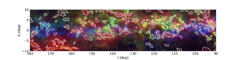
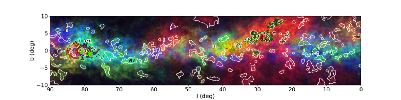
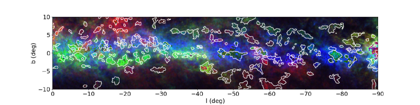
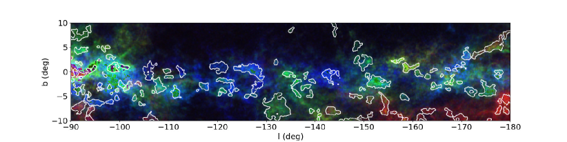
Figure 1: Distributions of the molecular clouds identified in the current work in the Galactic coordinates. The background three-colour composite images illustrate the three-dimensional distributions of dust in the Galactic disk from Paper I. Red, green and blue scales show the distributions of the colour excess $\delta$$E(G_{\rm BP}-G_{\rm RP})$ in distance slices 0 - 1000 pc, 1000 - 2000 pc and 2000 - 5000 pc from the Sun, respectively. The white polygons mark the $l$ and $b$ boundaries of the individual molecular clouds identified in the current work.

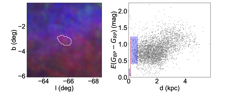
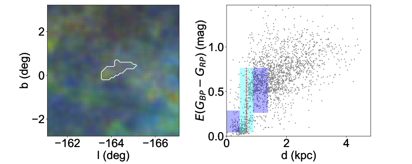
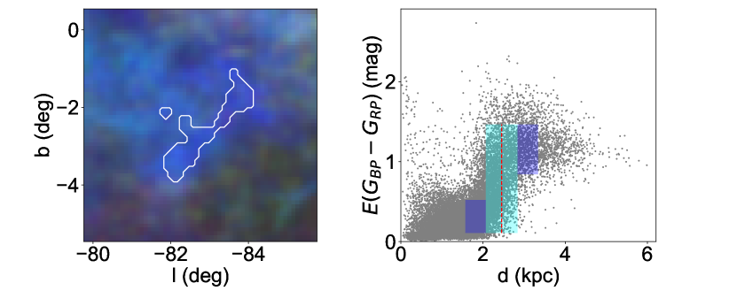
Figure 2: Distances to clouds No. 61 (upper panels), 318 (middle panels) and 539 (bottom panels). In the left panels, red, green and blue scales show the distributions of the colour excess $\delta$$E(G_{\rm BP}-G_{\rm RP})$ in distance slices 0 - 1000 pc, 1000 - 2000 pc and 2000 - 5000 pc from the Sun, respectively. White polygons show the region of sky of the clouds and from which the stars used in the distance determination are drawn. In the right panels, the values of colour excess $E(G_{\rm BP}-G_{\rm RP})$ of the selected stars are plotted against distances of the stars. The rectangles show the best-fit colour excess profiles. In each panel, the cyan rectangle represents the width of the cloud ($\delta d$) and the blue rectangles show the 1$\sigma$ regions of the foreground and background colour excesses of the cloud. The red dashed lines show the distances of the clouds.

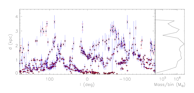
Figure 3: Derived cloud distances plotted against their Galactic longitudes. The red and blue error-bars show the distance uncertainties and the derived width/depth ($\delta d$) of the clouds, respectively. Also shown to the right of the panel is the distribution of the estimated total masses of the molecular clouds in the individual distance bins of width 0.2 kpc.

Table 1: Catalogue of molecular clouds.

ID	$l$	$b$	$\Omega$	$r$	$d_{0}$	$\delta d$	$\overline{E(G_{\rm BP}-G_{\rm RP})}$	$M$	$\Sigma$
	($\degr$)	($\degr$)	(deg2)	(pc)	(pc)	(pc)	(mag)	($M_{\odot}$)	$(M_{\odot}$ pc2)
1	177.727	$-$9.596	0.730	1.3	149.3$\pm$3.5	10.2$\pm$0.2	0.80	248.5	50.1
2	175.715	$-$9.651	1.903	1.1	78.9$\pm$1.9	10.0$\pm$0.2	0.97	218.5	60.6
3	170.131	$-$8.972	5.749	3.8	160.8$\pm$3.8	51.6$\pm$1.2	0.99	2787.5	61.5
4	107.778	$-$9.278	2.517	7.3	467.8$\pm$11.0	192.1$\pm$4.5	0.36	3723.7	22.2
5	94.961	$-$9.339	5.607	12.4	531.7$\pm$12.5	128.2$\pm$5.5	0.37	11205.9	23.2
6	32.797	$-$8.898	4.773	5.5	254.3$\pm$6.0	90.6$\pm$2.1	0.64	3746.5	39.9
7	11.421	$-$9.357	2.704	2.8	173.1$\pm$4.1	52.2$\pm$1.2	0.51	787.4	31.9
8	$-$52.953	$-$9.019	4.839	0.9	41.7$\pm$1.0	10.0$\pm$0.2	0.33	52.9	20.6
9	$-$59.581	$-$8.908	8.982	3.5	117.5$\pm$2.8	38.3$\pm$0.9	0.47	1103.2	29.2
10	$-$93.764	$-$9.628	1.242	3.9	355.6$\pm$8.4	40.7$\pm$4.0	0.52	1540.3	32.2
…	…	…	…	…	…	…	…	…	…
560	$-$68.358	$-$1.273	0.760	25.3	2942.1$\pm$69.4	241.1$\pm$83.1	0.60	75291.7	37.6
561	12.740	$-$1.095	0.400	20.4	3269.0$\pm$214.5	422.1$\pm$142.0	0.36	28886.7	22.2
562	$-$73.360	$-$0.551	0.420	19.2	3012.1$\pm$109.1	233.4$\pm$111.1	0.55	39587.5	34.1
563	$-$73.759	0.128	0.350	17.9	3065.8$\pm$98.7	239.2$\pm$108.8	0.56	34729.9	34.7
564	$-$69.328	1.674	1.139	34.8	3313.7$\pm$78.2	377.1$\pm$61.7	0.27	64708.4	17.0
565	$-$105.961	0.176	5.859	86.1	3612.7$\pm$85.3	481.5$\pm$36.6	0.33	473619.1	20.3
566	$-$65.300	$-$0.325	0.410	20.5	3256.2$\pm$117.4	374.5$\pm$79.6	0.56	46280.5	35.0
567	87.082	$-$0.151	1.830	48.3	3625.5$\pm$85.6	460.9$\pm$38.8	0.36	166119.2	22.7

The Table is available in its entirety in machine-readable form in the online version of this manuscript and also at the website
“http://paperdata.china-vo.org/diskec/dustcloud/table1.txt”.

In the current work, we have identified 567 molecular clouds with program Dendrogram. The distribution of the clouds, catalogued in Table 1, in Galactic coordinates $l$ and $b$ is presented in Fig. 1. The typical solid angle subtended by a cloud is about 1.5 deg². Typically there are $\sim$4,500 stars along the sightlines toward a cloud in the C19 Sample.

4.1 Distances of the molecular clouds

Fig. 2 shows the results of our colour excess profile fitting procedure for three example molecular clouds. In general, the values of colour excess $E(G_{\rm BP}-G_{\rm RP})$  of stars in individual distance bins show significant dispersions, as those stars cover quite a large area ($\sim$ 1 $-$ 2 deg²). However, the “jumps” in colour excess values produced by the molecular clouds in the corresponding distance ranges given by program Dendrogram are clearly visible. They are nicely fitted by our colour excess profiles.

The panels in the first row of Fig. 2 show the fitting analysis of a nearby molecular cloud with distance $d$ of 127 pc from the Sun. Due to the saturation of the photometric data used in Paper I, there are only a few stars in the C19 Sample that are located in front of the cloud. The quality of colour excess profile fit for the cloud is relatively poor compared to that of more distant clouds.

The panels in the second and third rows of Fig. 2 show examples of two clouds located respectively at distances 659 pc and 2,453 pc from the Sun. Compared to the nearby molecular cloud, the distance ranges of the colour excess jumps of more distant molecular clouds are larger. As a result, more distant clouds have larger ‘widths’ ($\delta d$). This is mainly caused by the larger distance errors of stars at further distances. If one assumes that the molecular clouds are spherical, the intrinsic widths of the clouds range between $\sim$ 1-100 pc (see Sect. 4.2). On the other hand, the typical uncertainties of the Gaia parallaxes for stars at distances of 2 kpc are $\sim$10 per cent, i.e. $\sim$ 200 pc, which is twice of the upper limit of the intrinsic widths of the clouds. Therefore, the resulted values of width $\delta d$ for distant clouds are mainly contributed by the distance errors of the individual stars. However, benefiting from the large numbers of stars for the individual clouds, the large distance uncertainties do not have significant impacts on the distance determinations of the clouds.

In directions toward some molecular clouds, we are able to see more than one colour excess jump. The additional jumps are produced by the foreground or background clouds. With the distance ranges provided by Dendrogram, we are able to exclude the contamination of those foreground or background clouds and obtain accurate distances for the individual identified clouds.

For each molecular cloud identified in the current work, we have made figures analogous to Fig. 2. They are available online. The best-fit values and uncertainties of distances $d_{0}$ and width $\delta d$, and the averaged colour excess $\overline{E(G_{\rm BP}-G_{\rm RP})}$ of the individual catalogued clouds are listed in Table 1. Fig. 3 plots the centre longitude $l$ of all the molecular clouds against their distances $d_{0}$. The associated statistical distance uncertainties and the estimated widths (depths) of the clouds ($\delta d$) are also overplotted. The cloud range in distances from $d_{0}\approx 30$ pc to $\sim 4,000$ pc. The catalogue should be complete between 1 and 3 kpc. For distances larger than 3 kpc, our sample is incomplete due to the limited depth of the adopted 3D colour excess maps, while for distances closer than 1 kpc, it is incomplete mainly due to the incomplete coverage of Galactic latitudes of the dataset. In addition, we note that the far-away clouds would appear be stretched due to the relatively large distance errors. Their observed differential colour excesses [$d$$E(G_{\rm BP}-G_{\rm RP})$$/ds$, where $s$ is the distance] are actually smaller than the intrinsic values. Thus the far-away clouds with low dust density could be under our detection threshold. At larger distances, our selection procedure might have missed those low density clouds or the low density parts of the clouds. Owing to the accurate distances of stars yielded by the Gaia parallaxes and the large numbers of stars available to trace the individual clouds, we have achieved a very high precision for our distance estimates of the clouds. Most of the clouds in our catalogue have relative distance uncertainties smaller than 5 per cent. The typical ‘width (depth)’ of the catalogued clouds is about 18 per cent of the distance values, largely caused by the distance errors of the individual stars used to trace the clouds.

4.2 Physical properties

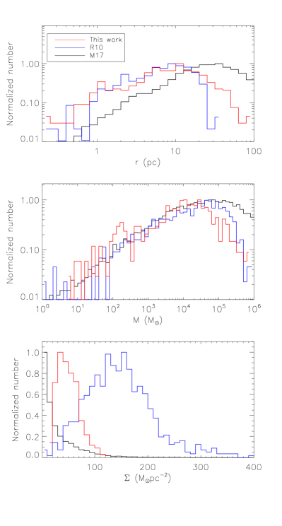
Figure 4: Histograms of the physical properties radii (upper panel), masses (middle panel) and surface mass densities (bottom panel) of the molecular clouds catalogued in the current work (red lines), and those in Roman-Duval et al. (2010, blue lines) and Miville-Deschênes et al. (2017, black lines).

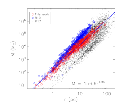
Figure 5: The masses plot against the radii for the molecular clouds in the current work (red circles), that of Roman-Duval et al. (2010, blue squares) and Miville-Deschênes et al. (2017, black dots). The blue line is the best-fit correlation of the mass of the molecular clouds in our work and their radii.

The derived physical properties, such as the physical radius $r$, mass $M$ and surface mass density $\Sigma$, of the molecular clouds are also listed in Table. 1. Fig. 4 plots the histograms of those properties. The radii of the clouds range between 0.2 and 90 pc with a median value of $\sim$ 8 pc, the masses between 5 and 700,000 $M_{\odot}$ with a median value of $\sim$ 10,000 $M_{\odot}$ and the surface mass densities between 10 and 125 $M_{\odot}$ pc² with a median value of $\sim$ 50 $M_{\odot}$ pc².

The distributions of the corresponding properties of clouds studied by Roman-Duval et al. (2010) and Miville-Deschênes et al. (2017) are also overplotted in Fig. 4 for comparison. Roman-Duval et al. (2010) have derived physical properties of 580 molecular clouds based on the CO observations of the University of Massachusetts-Stony Brook (UMSB) and Galactic Ring surveys. Miville-Deschênes et al. (2017) have isolated 8,107 molecular clouds from the CO observations of Dame et al. (2001) and derived their physical properties. The molecular clouds of Roman-Duval et al. (2010) and Miville-Deschênes et al. (2017) cover disk regions which are of much further distances from the Sun than those catalogued here. In addition, their physical properties are obtained from data with methods much different from ours. Nevertheless, the resultant distributions of the physical radii and masses of the molecular clouds are very similar, suggesting that the structures identified in the current work are essentially the same type of object as those identified in those previous studies.

Fig. 5 shows the correlation between the radii and masses of the molecular clouds. The radii and masses of our molecular clouds are tightly correlated by a power-law, $M=156.6R^{1.96}$. The exponent index 1.96, which corresponds to a typical surface density of $\sim$ 50 $M_{\odot}$ pc², is slightly smaller than that found by Roman-Duval et al. (2010) but consistent with that of Miville-Deschênes et al. (2017). This limiting surface density is largely caused by the fact that we have imposed a limiting extinction to our sample sources (Sect. 3).

The estimation of cloud masses and radii depends on how the cloud boundaries are defined. The differences in cloud mass-size distributions reported in different work are most likely caused by the different criteria used to define the clouds.

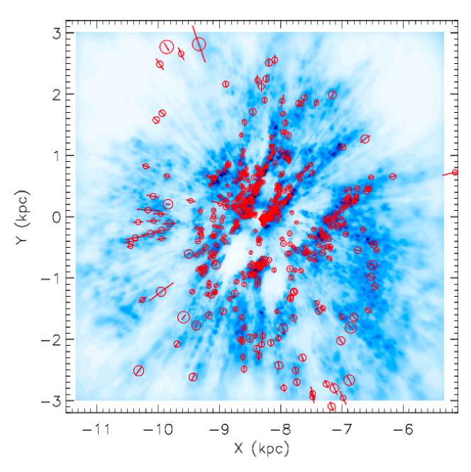
Figure 6: Spatial distribution of the molecular clouds identified and catalogued in the current work (circles) in the $X$-$Y$ plane, plotted over the distribution of the Galactic dust of disk vertical height $|Z|$ $<$ 0.4 kpc (blue scales; Lallement et al. 2019). The sizes of the circles are proportional to the physic sizes of the individual clouds and the error-bars indicate their distance uncertainties. The Sun, assumed to be at the position of ($X,~{}Y,~{}Z$) = ($-$8.34, 0, 0) kpc, is located at the centre of the plot.

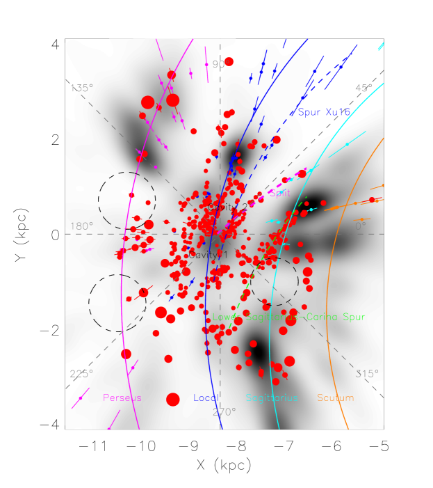
Figure 7: Spatial distribution of the identified molecular clouds in the $X$-$Y$ plane. The sizes of the circles are proportional to the physic sizes of the individual clouds and the error-bars indicate their distance uncertainties. Solid orange, cyan, blue and pink lines delineate the best-fit spiral arm models of the Sagittarius, Local and Perseus Arms presented in Chen et al. (2019a). Circles of the aforementioned colours are the masers from Xu et al. (2018) that are probably associated with the individual Arms. The grey background image represents the spatial distribution of the OB stars from Chen et al. (2019a). The green, pink and blue dashed lines mark respectively a possible spur ‘Lower Sagittarius-Carina Spur’, the ‘split’ found by Lallement et al. (2019) and the spur identified by Xu et al. (2016). Three black dashed circles mark the positions of three possible ‘hole’ patterns in the Sagittarius and Perseus Arms identified in Chen et al. (2019a). The Sun, assumed to be at the position of ($X,~{}Y,~{}Z$) = ($-$8.34, 0, 0) kpc, is located at the centre of the plot. The directions of $l$ = 0°, 45°, 90°, 135°, 180°, 225°, 270° and 315° are also marked in the plot.

5 Discussion

Table 2: Comparison of distances of molecular clouds with the literature values.

Name	ID	$l$	$b$	$d_{0}$	Literature $d_{0}$
		($\degr$)	($\degr$)	(pc)	(pc)
California	187	161.101	-8.922	451.2$\pm$10.6	410$\pm$41a, 470$\pm$26b,450$\pm$23c
California	189	158.282	-8.578	473.2$\pm$11.2	410$\pm$41a, 470$\pm$26b,450$\pm$23c
California	235	163.883	-8.380	439.3$\pm$10.4	410$\pm$41a, 470$\pm$26b,450$\pm$23c
Cepheus	353	106.260	9.687	1047.8$\pm$24.7	900$\pm$90a, 923$\pm$47b, 1043${}^{+6}_{-7}$d
Hercules	153	44.593	8.882	208.7$\pm$4.9	200$\pm$30a, 227$\pm$12b, 229${}^{+4}_{-3}$d
Pipe Nebula	115	0.891	4.131	155.2$\pm$3.7	130$\pm$15e, 145$\pm$16f
Pipe Nebula	128	-1.200	5.446	159.5$\pm$3.8	130$\pm$15e, 145$\pm$16f
Pipe Nebula	143	-2.324	6.551	113.3$\pm$2.7	130$\pm$15e, 145$\pm$16f
Circinus	242	-42.343	-4.054	819.2$\pm$19.3	700$\pm$350g
CMa OB1	366	-137.931	-3.109	1217.8$\pm$28.7	1456$\pm$146a, 1209$\pm$64b,1150$\pm$64h
CMa OB1	402	-136.195	-4.325	1225.8$\pm$28.9	1456$\pm$146a, 1209$\pm$64b,1150$\pm$64h
CMa OB1	414	-136.119	-2.153	1265.3$\pm$29.9	1456$\pm$146a, 1209$\pm$64b,1150$\pm$64h
Maddalena	529	-142.675	-1.063	2026.4$\pm$243.4	2350$\pm$235a, 2072$\pm$110b
Maddalena	544	-144.632	-0.413	2353.4$\pm$73.7	2350$\pm$235a, 2072$\pm$110b
Mon R2	233	-147.177	-9.806	866.7$\pm$20.5	952$\pm$95a, 778$\pm$42b, 905$\pm$37h
Mon OB1	319	-159.166	0.885	791.0$\pm$18.7	890$\pm$89a, 745$\pm$40b
Orion Lam	12	-170.023	-9.455	408.4$\pm$9.6	427$\pm$43a, 402$\pm$21b, 445$\pm$50h
Orion Lam	14	-161.521	-9.236	406.9$\pm$9.6	427$\pm$43a, 402$\pm$21b, 445$\pm$50h
Orion Lam	25	-163.075	-8.053	409.2$\pm$9.7	427$\pm$43a, 402$\pm$21b, 445$\pm$50h
Orion Lam	188	-167.414	-8.462	383.9$\pm$9.1	427$\pm$43a, 402$\pm$21b, 445$\pm$50h

References: ^aSchlafly et al. (2014), ^bZucker et al. (2019), ^c Lada et al. (2009), ^dYan et al. (2019), ^eLombardi et al. (2006), ^fAlves & Franco (2007), ^gBally et al. (1999), ^hLombardi et al. (2011).

5.1 Comparison with previous work

The unique catalogue presented in the current work is one of the largest homogeneous catalogues of molecular clouds with accurate distance estimates. The clouds span in distances from $\sim$30 to $\sim$4,000 pc, with typical uncertainties of less than 5 pre cent. To verify the robustness of our distance estimates, we have selected some well studied giant molecular clouds and collect their distance estimates from the literature. The results are listed in Table 2. Overall, our values agree well with those from the literature.

For some nearby giant molecular cloud complexes, such as the California, Pipe Nebula, CMA OB1 and Orion Lam, we have isolated more than one clouds in each of them. The resulted distance estimates of the individual clouds are consistent with each others within 3$\sigma$. There are also some molecular clouds that have extended to the medium or high Galactic latitudes, such as the Orion Lam, Mon R2, Hercules, etc. We have been only able to identify parts of them, limited by the latitude coverage of our data ($b$ $<$ 10°). Nevertheless, our estimated distances are in good agreement with those in the literature. The Cepheus Flare, for example, is a structure complex that contains at least two components (Kun et al., 2008; Schlafly et al., 2014). As the footprint of our data are limited to Galactic latitudes smaller than 10°, we are only able to identified parts of its southern component, named cloud No. 353 in the current work. It is centered at $l$ = 106.260° and $b$ = 9.687° and have a distance of 1047.8$\pm$24.7 pc. Literature estimates of distance for this component are 900$\pm$90 pc (Schlafly et al., 2014), 923$\pm$47 pc (Zucker et al., 2019) and 1043${}^{+6}_{-7}$ pc (Yan et al., 2019), all in good agreement with our current result. The dispersion of differences between our distance estimates and those from Zucker et al. (2019) and Yan et al. (2019) is about 5.6 per cent. Note that all the cloud distances here are derived from Gaia DR2 parallaxes.

We also compare the spatial distribution of our molecular clouds to the 3D dust distribution of the Galactic plane from Lallement et al. (2019). Based on the photometric data of Gaia DR2 and 2MASS, and the parallaxes of Gaia DR2, Lallement et al. (2019) present the 3D distribution of the interstellar dust in a volume of 6 $\times$ $6$ $\times$ 0.8 kpc³ around the Sun with a hierarchical inversion algorithm. The comparison is shown in Fig. 6. The spatial distribution of the molecular clouds catalogued here is in excellent agreement with the dust distribution of Lallement et al. (2019). The good agreement validates the robustness of methods used in both papers.

5.2 The Galactic spiral structure as traced by the molecular clouds

As Figs. 3 and 6 show, the molecular clouds in our catalogue trace clearly the large-scale structure of the Galactic disk, i.e., the spiral arms. The gaps between the different arms are quite visible.

In Fig. 7, we plot the spatial distribution of the molecular clouds in the $X$-$Y$ plane. The distributions of masers (Table 2 of Xu et al. 2018) and young OB stars and candidates (Chen et al., 2019a) are over-plotted in the diagram. Chen et al. (2019a) have estimated structure parameters of the Scutum, Sagittarius, Local and Perseus Arms based on their sample of O and early B-type stars and the maser sample of Xu et al. (2018). Overall, the molecular clouds catalogued here are very likely to be spatially associated with the arms delineated by Chen et al. (2019a).

The Perseus Arm is well traced by the molecular clouds, the masers and the OB stars in the outer disk, for longitudes between 90° and 230°. The Perseus Arm is quite a diffuse arm. Based on the spatial distribution of the OB stars and masers, Chen et al. (2019a) identify two possible ‘hole’ patterns within the Arm with no masers and few OB stars. The molecular clouds identified here around the two ‘holes’ are also fragmented, albeit with a different pattern. A significant fraction of the clouds concentrated in the direction of the Galactic anti-centre ($l$ $\sim$ 180°), where the masers and OB stars also clump. Although several molecular clouds are visible in the two ‘holes’ repoted by Chen et al. (2019a), the ‘holes’ are less populated by the clouds than in other areas.

Two significant cavities are visible in the Solar neighborhood. Cavity 1 (Chen et al., 2014; Lallement et al., 2019) falls in the direction $l$ $\sim$ 240° and Cavity 2, which is smaller, in $l$ $\sim$ 60°. The model line of the Local arm, derived from the OB stars and masers, goes along the upper boundary of Cavity 2, and through the centre of Cavity 1. The lower boundaries of the two cavities seem to be the foreground structure of the spur identified by Xu et al. (2016) that connects the Local and the Sagittarius Arms at a pitch angle of $\sim$ 18° (the blue dashed line in Fig. 7). On the other hand, those nearby molecular clouds around $l$ $\sim$ 45° seem also to be the foreground clouds of the so-called ‘split’ (Lallement et al., 2019) that connects the Local and the Sagittarius Arms at a pitch angle of $\sim$ 48° (the pink dashed line in Fig. 7).

Due to the significant amount of foreground dust extinction, we have not been able to identify the molecular clouds of the Sagittarius Arm in the direction of $l$ between 30° and 45°. The molecular clouds located in the directions of $l$ $\sim$ 15° ($X$ $\sim$ $-$6.8 kpc and $Y$ $\sim$ 0.5 kpc) and $l$ $\sim$ 285° ($X$ $\sim$ $-$7.5 kpc and $Y$ $\sim$ $-$2.5 kpc) seems to be parts of the Sagittarius Arm. Similar to the distribution of OB stars, no molecular clouds are found in the ‘hole’ of the Sagittarius Arm identified by Chen et al. (2019a). Another significant feature is a structure of $\sim$ 3 kpc length that connects the the Local and the Sagittarius Arms at a pitch angle of $\sim$ 34° (the green dashed line in Fig. 7). This structure is apparent in the previous 3D extinction maps such as Chen et al. (2019b) and Lallement et al. (2019). It was treated as a cloud complex and was labelled as “Lower Sagittarius-Carina” in Lallement et al. (2019). However, it could be a new spur of the Galactic spiral structure and we call it “Lower Sagittarius-Carina Spur”. Chen et al. (2019c) have reported a massive star-forming region G352.630-1.067 and suggest that it may be located in a spur extending from the Sagittarius Arm close to the direction of Galactic centre. The distance of G352.630-1.067 is 0.69 kpc. It is much closer than the new spur found in the current work which have a distance of about 1.1 kpc in the direction. A detail analysis of this new spur will be presented in a future work (Li et al. 2020, in preparation).

6 Conclusion

In this paper, we have presented a new, large and homogeneous catalogue of 567 molecular clouds within 4 kpc from the Sun at low Galactic latitudes ($|b|$ $<$ 10°) using the data presented in Paper I. The molecular clouds are identified by a dendrogram analysis of the 3D colour excess maps of the Galactic disk. Based on the previous determinations of extinction values and distances of over 32 million stars, we have derived accurate distances of those molecular clouds by analyzing the colour excess and distance relations along the sightlines of the individual clouds. The typical errors of the distances are less than 5 pre cent. As far as we know, the resulted catalogue is the first large catalogue of molecular clouds with directly-measured distances in the Galactic plane.

We have also measured the areas, the linear equivalent radii, the masses and the surface mass densities of the catalogued molecular clouds. A tight power-law correlation of index 1.96, is found between the radii and masses.

We have explored the distribution of our clouds in the Galactic disk, and studied the connection between the dust distribution and the spiral arms. Broadly speaking, the molecular clouds are found to be spatially associated with the Galactic spiral arm models delineated in the previous work (Chen et al., 2019a), where on smaller scales, spur-like structures are not uncommon. In this respect, we have identified a possible spur, the “Lower Sagittarius-Carina Spur”, with a pitch angle of about 34° that connects the Local and the Sagittarius Arms in the fourth quadrant.

References

- Alves & Franco (2007) Alves, F. O. & Franco, G. A. P. 2007, A&A, 470, 597
- Bailer-Jones et al. (2018) Bailer-Jones, C. A. L., Rybizki, J., Fouesneau, M., Mantelet, G., & Andrae, R. 2018, AJ, 156, 58
- Bally et al. (1999) Bally, J., Reipurth, B., Lada, C. J., & Billawala, Y. 1999, AJ, 117, 410
- Blitz & Williams (1999) Blitz, L. & Williams, J. P. 1999, in NATO Advanced Science Institutes (ASI) Series C, ed. C. J. Lada & N. D. Kylafis, Vol. 540, 3
- Brand et al. (1994) Brand, J., et al. 1994, A&AS, 103, 541
- Chen et al. (2019a) Chen, B. Q., et al. 2019a, MNRAS, 487, 1400
- Chen et al. (2019b) Chen, B. Q., et al. 2019b, MNRAS, 483, 4277
- Chen et al. (2017) Chen, B. Q., et al. 2017, MNRAS, 472, 3924
- Chen et al. (2015) Chen, B. Q., Liu, X. W., Yuan, H. B., Huang, Y., & Xiang, M. S. 2015, MNRAS, 448, 2187
- Chen et al. (2014) Chen, B. Q., et al. 2014, MNRAS, 443, 1192
- Chen et al. (2019c) Chen, X., Li, J.-J., Zhang, B., Ellingsen, S. P., Xu, Y., Ren, Z.-Y., Shen, Z.-Q., & Sobolev, A. M. 2019c, ApJ, 871, 198
- Dame et al. (2001) Dame, T. M., Hartmann, D., & Thaddeus, P. 2001, ApJ, 547, 792
- Dobashi (2011) Dobashi, K. 2011, PASJ, 63, S1
- Gaia Collaboration et al. (2018) Gaia Collaboration, et al. 2018, A&A, 616, A1
- García et al. (2014) García, P., Bronfman, L., Nyman, L.-Å., Dame, T. M., & Luna, A. 2014, ApJS, 212, 2
- Goodman et al. (2014) Goodman, A. A., et al. 2014, ApJ, 797, 53
- Goodman et al. (2009) Goodman, A. A., Pineda, J. E., & Schnee, S. L. 2009, ApJ, 692, 91
- Green et al. (2015) Green, G. M., et al. 2015, ApJ, 810, 25
- Kun et al. (2008) Kun, M., Kiss, Z. T., & Balog, Z. 2008, Star Forming Regions in Cepheus, ed. B. Reipurth, Vol. 4, 136
- Lada et al. (2009) Lada, C. J., Lombardi, M., & Alves, J. F. 2009, ApJ, 703, 52
- Lallement et al. (2019) Lallement, R., Babusiaux, C., Vergely, J. L., Katz, D., Arenou, F., Valette, B., Hottier, C., & Capitanio, L. 2019, A&A, 625, A135
- Li et al. (2016) Li, G.-X., Urquhart, J. S., Leurini, S., Csengeri, T., Wyrowski, F., Menten, K. M., & Schuller, F. 2016, A&A, 591, A5
- Li et al. (2013) Li, G.-X., Wyrowski, F., Menten, K., & Belloche, A. 2013, A&A, 559, A34
- Lindegren et al. (2018) Lindegren, L., et al. 2018, A&A, 616, A2
- Lombardi et al. (2006) Lombardi, M., Alves, J., & Lada, C. J. 2006, A&A, 454, 781
- Lombardi et al. (2011) Lombardi, M., Alves, J., & Lada, C. J. 2011, A&A, 535, A16
- Magnani et al. (1985) Magnani, L., Blitz, L., & Mundy, L. 1985, ApJ, 295, 402
- Markwardt (2009) Markwardt, C. B. 2009, in Astronomical Society of the Pacific Conference Series, Vol. 411, Astronomical Data Analysis Software and Systems XVIII, ed. D. A. Bohlender, D. Durand, & P. Dowler, 251
- Marshall et al. (2009) Marshall, D. J., Joncas, G., & Jones, A. P. 2009, ApJ, 706, 727
- May et al. (1997) May, J., Alvarez, H., & Bronfman, L. 1997, A&A, 327, 325
- Miville-Deschênes et al. (2017) Miville-Deschênes, M.-A., Murray, N., & Lee, E. J. 2017, ApJ, 834, 57
- Moré (1978) Moré, J. J. 1978, The Levenberg-Marquardt algorithm: Implementation and theory, Vol. 630, 105–116
- Nakagawa et al. (2005) Nakagawa, M., Onishi, T., Mizuno, A., & Fukui, Y. 2005, PASJ, 57, 917
- Roman-Duval et al. (2009) Roman-Duval, J., Jackson, J. M., Heyer, M., Johnson, A., Rathborne, J., Shah, R., & Simon, R. 2009, ApJ, 699, 1153
- Roman-Duval et al. (2010) Roman-Duval, J., Jackson, J. M., Heyer, M., Rathborne, J., & Simon, R. 2010, ApJ, 723, 492
- Rosolowsky et al. (2008) Rosolowsky, E. W., Pineda, J. E., Kauffmann, J., & Goodman, A. A. 2008, ApJ, 679, 1338
- Schlafly et al. (2014) Schlafly, E. F., et al. 2014, ApJ, 786, 29
- Schlafly et al. (2015) Schlafly, E. F., et al. 2015, ApJ, 799, 116
- Skrutskie et al. (2006) Skrutskie, M. F., et al. 2006, AJ, 131, 1163
- Wang et al. (2015) Wang, K., Testi, L., Ginsburg, A., Walmsley, C. M., Molinari, S., & Schisano, E. 2015, MNRAS, 450, 4043
- Wright et al. (2010) Wright, E. L., et al. 2010, AJ, 140, 1868
- Xu et al. (2018) Xu, Y., Hou, L.-G., & Wu, Y.-W. 2018, Research in Astronomy and Astrophysics, 18, 146
- Xu et al. (2016) Xu, Y., et al. 2016, Science Advances, 2, e1600878
- Yan et al. (2019) Yan, Q.-Z., Zhang, B., Xu, Y., Guo, S., Macquart, J.-P., Tang, Z.-H., & Walsh, A. J. 2019, A&A, 624, A6
- Yu et al. (2019) Yu, B., Chen, B. Q., Jiang, B. W., & Zijlstra, A. 2019, MNRAS, 488, 3129
- Zucker et al. (2019) Zucker, C., Speagle, J. S., Schlafly, E. F., Green, G. M., Finkbeiner, D. P., Goodman, A. A., & Alves, J. 2019, ApJ, 879, 125