QoS-aware Stochastic Spatial PLS Model for Analysing Secrecy Performance under Eavesdropping and Jamming

Abstract

Securing wireless communication, being inherently vulnerable to eavesdropping and jamming attacks, becomes more challenging in resource-constrained networks like Internet-of-Things. Towards this, physical layer security (PLS) has gained significant attention due to its low complexity. In this paper, we address the issue of random inter-node distances in secrecy analysis and develop a comprehensive quality-of-service (QoS) aware PLS framework for the analysis of both eavesdropping and jamming capabilities of attacker. The proposed solution covers spatially stochastic deployment of legitimate nodes and attacker. We characterise the secrecy outage performance against both attacks using inter-node distance based probabilistic distribution functions. The model takes into account the practical limits arising out of underlying QoS requirements, which include the maximum distance between legitimate users driven by transmit power and receiver sensitivity. A novel concept of eavesdropping zone is introduced, and relative impact of jamming power is investigated. Closed-form expressions for asymptotic secrecy outage probability are derived offering insights into design of optimal system parameters for desired security level against the attacker’s capability of both attacks. Analytical framework, validated by numerical results, establishes that the proposed solution offers potentially accurate characterisation of the PLS performance and key design perspective from point-of-view of both legitimate user and attacker.

I Introduction

Wireless communication owing to its open and broadcast nature is highly vulnerable to eavesdropping and jamming attacks. Recently, physical layer security (PLS) has recently drawn remarkable attention of the researchers in resources constrained wireless networks like Internet of Things (IoT) [2]. Various PLS techniques have been reported in the literature with a major focus on eavesdropping attack and friendly jamming. Here, legitimate nodes leverage the interference to secure the communication and the attacker is restricted to act as a mere passive adversary [3, 4, 5, 6, 7]. However, the attacker may also use the interference to its advantage by jamming the legitimate reception other than eavesdropping. It is, therefore, of interest to study the attacker in both eavesdropping and jamming modes. Furthermore, spatial configurations of legitimate nodes and attackers are, in general, modelled in deterministic manner. This assumption is only valid if the location of the node is known. Therefore, appropriate modelling of a stochastic network is needed to investigate the critical role of random inter-node separations on secrecy performance when the exact location information is not available.

I-A Related Art

PLS is extensively explored to analyse secrecy capacity (SC) and secrecy outage probability (SOP) in various scenarios including High SNR regime [8, 9, 10, 11]. In [9], artificial noise is exploited to enhance security in multiple-input single-output non-orthogonal multiple access (MISO-NOMA) systems by developing a secrecy beamforming scheme. Impact of imperfect channel state information (CSI) is also widely explored in analysing the network performance [10, 11] when perfect CSI is not available. However, these works ignored the randomness caused by large-scale propagation losses. There is another line of research exploring the secure communication in spatial stochastic networks [12, 13, 14, 15]. These works explore the secrecy performance under a passive eavesdropper assuming the spatial distribution of the nodes as a homogeneous Poisson Point Process (PPP) which may be a good approximation for large-scale networks with known network density. The stationary and isotropic properties of homogeneous PPP consider that characteristics of network as viewed from a node’s aspect are similar for all the nodes. However, this assumption is not valid in practical networks, especially having a finite number of nodes within a given area [16]. Further, it is incapable of analysing the average performance measures at a randomly deployed node which has significant importance in realistic networks. Some scenarios showing limitations of above models under Device-to-Device (D2D) or sensor networks has been examined in [17, 18].

Apart from aforementioned works, studies in [19, 20, 21] exhibit a recent research interest on hybrid attackers that can either eavesdrop or jam. The authors have investigated the full duplex attacker in [22, 23] where passive eavesdropping and active jamming are performed simultaneously. In [24] secrecy performance of a wireless network with randomly deployed hybrid attackers is analysed using stochastic geometry tools and random matrix theory. Recently, much attention is being paid to the utilisation of distance distributions as a complement to PPP models for performance analysis in wireless networks [17, 18] without considering secrecy requirements.

I-B Research Gap and Motivation

As noted in the literature survey, PLS in spatial stochastic networks is mainly studied under the assumption of homogeneous PPP based deployment of nodes [12, 13, 14, 15, 24] which are non-viable in several practical scenarios [17, 18]. Moreover, most studies of stochastic networks consider a passive attacker that can only eavesdrop. Recently, works in [19, 20, 21] have shown the growing interest in hybrid attackers. But, above-mentioned works consider the deterministic path-loss. The authors in [24] have studied the hybrid attacker considering random path-loss, however, analysis is done under the PPP assumption and available perfect CSI of the users to the source. These observations reveal that secrecy analysis in a spatial stochastic network for a general scenario under eavesdropping as well as jamming mode of the attacker is still an open research problem. In practical networks including IoT and D2D, legitimate nodes as well as attacker may be deployed randomly in the deployment regions; consequently, the exact location of any node may not be available. Furthermore, connection between two nodes will be set up when the geographical separation between them is smaller than a predefined threshold for retaining Quality-of-Service (QoS). In a similar way, attacker’s capabilities to eavesdrop and jam also influence the secrecy performance; hence they are indirect measure of QoS attributes from attacker’s point of view. Eavesdropping capability is practically constrained by hardware limitations while jamming capability is constrained by power consumption. It is to be mentioned here that these QoS-governing parameters did not get due attention in literature. These facts motivate the study of this work for developing a practical and comprehensive stochastic model so as to quantify secrecy performance in a realistic manner.

I-C Key Contributions

This work, aimed at filling the mentioned research gap, has the following key contributions:

• We have proposed a novel generalised QoS-aware stochastic spatial PLS to investigate secrecy analysis in the presence of an attacker with both capabilities- eavesdropping and jamming. Here, the key aspect is that our model allows any arbitrary location for nodes within the deployment region (Section 2).

• First-time characterisation of attacker’s eavesdropping capability is provided in terms of novel eavesdropping zone concept. The proposed model also incorporates the restriction being imposed on the maximum distance between legitimate nodes arising out of the underlying QoS requirement. Considering these practical constraints, the distribution functions of the distances and SNRs of legitimate, eavesdropping and jamming links are derived. Closed-form expressions are also derived for ratio distributions of legitimate-to-attacker link SNRs. This is a vital figure of merit being applied to derive the secrecy performance measures (Section 3).

• Using probabilistic distance based distributions, we obtain expression for secrecy outage probability having considered attacker’s eavesdropping capability. As such distribution functions could be used in a class of generalised practical scenarios. We also derived closed-form expressions for SOP in asymptotic scenario (Section 4).

• Probabilistic characterisation of secrecy outage is also provided having considered attacker’s jamming capability. For this case also, SOP is derived in closed-form for asymptotic case (Section 4).

• A generalised framework is provided for different possible deployment configurations for legitimate nodes and attacker. Also, novel and significant analytical insights about designing of different system parameters are provided under eavesdropping and jamming attacks. Maximum allowed separation between legitimate nodes are determined for achieving desired secrecy performance from the user’s perspective, while the optimal value of eavesdropping range and jamming power are investigated from the attacker’s perspective. (Section 5).

• Numerical results validate the proposed analysis and present secrecy-aware key design perspective by analysing the impact of inter-node distances on secrecy performance. The relative severity of eavesdropping and jamming capabilities of attacker are also compared. It is shown that attacker must have more transmit power than legitimate source to create more adverse conditions during jamming as compared to eavesdropping provided that it is capable to eavesdrop in entire deployment range (Section 6).

I-D Novelty and Scope

To the best of our knowledge, this is the first work that adopts a probabilistic distance-based practical model with consideration of the real-time constraints in terms of QoS-controlling parameters for secrecy analysis under eavesdropping as well as jamming. We also propose eavesdropping zone concept to incorporate the effect caused by eavesdropping capability of attacker and present novel analysis on the impact of stochastic inter-node distances on secrecy outage.

Scope of this work includes, though not limited to, development of a system with desired secrecy performance by exploiting the randomness of inter-node distances. This work, providing insights on designing of parameters of legitimate nodes and attacker, can be extended to multiple-input multiple-output (MIMO) model. Directional beam-forming can be applied to enhance the secrecy further. Additional insights can also be obtained by considering different fading environments. Another important extension of the work may include the selection of appropriate attacking mode and optimisation of designing parameters of attacker with the objective of minimising the achievable secrecy transmission rate. Though the widespread utility of the derived closed-form expressions for secrecy analysis is constrained by high SNR, they provide lower bounds on SOP with the positive SC to give useful insights. There is a class of practical applications that can benefit from proposed designs. These include small cell networks, IoT networks, ad-hoc networks where nodes are deployed within a small cell area. Hence, the impacts of leakage due to wiretapping and interference due to jamming are much greater than noise in the channel.

II Proposed System Model

In this section, we present the proposed system model including the spatially stochastic network topology, QoS-aware PLS model, channel model along with link SNR and SC definitions for background setup of the problem for both eavesdropping and jamming modes of attacker.

II-A Network topology

We consider a secure communication IoT scenario comprising of uniformly deployed multiple source-user pairs, where each pair is allocated orthogonal resources in terms of a dedicated time slot, or set of sub-carriers. The ongoing communication is assumed to be under security threat from a hybrid attacker with half-duplex capability. It can over-hear ongoing transmission as an eavesdropper through wiretapping or can act as a jammer causing interference to the information flow [19, 20, 21]. It is further assumed to be present within deployment region with some statistical information about its location. However, the relative distances between source, user and attacker are unknown to each other exactly. Adopting this orthogonal multi-access IoT setup, we can focus on any randomly chosen source-user pair and investigate the impact of attacker’s presence on the ongoing secure transmission. It may be noted that this discussion and the proceeding analysis holds for any randomly-selected source-user pair. Here, such an information source $\mathcal{S}$ and legitimate user $\mathcal{U}$ are assumed to be spatially distributed with uniform distribution in deployment region of radius $R$. Whereas, the attacker $\mathcal{A}$ can be randomly located anywhere in the deployment region. Without loss of generality, we explore secrecy performance assuming $\mathcal{A}$ to be located at the origin, as depicted in Fig. 1. Novel investigations are carried out under eavesdropping and jamming mode separately. Here, $\mathcal{A}$ is also considered as an IoT device so as to invade the network with malicious intentions by disguising itself. Considering form-factor constraints and lower hardware complexity of IoT devices, all nodes, including attacker, are assumed to be equipped with a single antenna [25, 26, 27, 28].

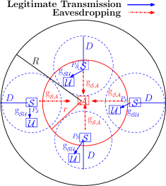
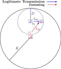
Figure 1: QoS-aware stochastic spatial PLS model with attacker in eavesdropping and jamming mode.

II-B QoS-Aware PLS Model

The proposed model investigates the PLS based secrecy metrics under eavesdropping as well as jamming. Here the phrase “QoS-aware” is associated with the obtaining of secrecy QoS requirements through critical design parameters of user as well as attacker from their respective point of view. These parameters include the distance threshold $D$, deployment range $R$ and source power $P_{\mathcal{S}}$ from the user’s perspective. On the other hand, attacker’s parameters like eavesdropping range $r$ and jamming power $P_{\mathcal{J}}$ also represent the capabilities to impact the network secrecy performance. Hence, they reflect the indirect measure of QoS attribute from attacker’s perspective. The proposed model first time characterises the secrecy performance by considering the real-world constraints in terms of these parameters defined by the underlying QoS requirements. Following this, the maximum possible geographical distance between $\mathcal{S}$ and $\mathcal{U}$ has been restricted to $D$ determined by the required QoS. The distance parameter $D$ is utilised to ensure the minimum QoS requirement over $\mathcal{S}$- $\mathcal{U}$ link. Further, for taking hardware limitations of $\mathcal{A}$ into account, we consider that under eavesdropping mode, the $\mathcal{A}$ remains effective in the disc area defined as eavesdropping zone with centre $\mathcal{A}$ and radius $r$. Here, $r$ is defined as the eavesdropping range of $\mathcal{A}$. It represents the maximum distance, to which $\mathcal{A}$ can eavesdrop the legitimate signal. We have categorised all possible deployment scenario of $\mathcal{S}$ and $\mathcal{U}$ with respect to $\mathcal{A}$’s eavesdropping zone into the four cases as illustrated in Fig. 1. These are:

• Case 1: Both $\mathcal{S}$ and $\mathcal{U}$ are deployed within the $\mathcal{A}$’s eavesdropping zone, i.e., ${d_{{}_{\mathcal{S}\mathcal{A}}}}<r$ and ${d_{{}_{\mathcal{U}\mathcal{A}}}}<r.$

• Case 2 : $\mathcal{S}$ is deployed within $\mathcal{A}$’s eavesdropping zone while $\mathcal{U}$ is outside, i.e., ${d_{{}_{\mathcal{S}\mathcal{A}}}}<r$ and $r\leq{d_{{}_{\mathcal{U}\mathcal{A}}}}<R.$

• Case 3 : $\mathcal{U}$ is deployed within $\mathcal{A}$’s eavesdropping zone while $\mathcal{S}$ is outside, i.e., $r\leq{d_{{}_{\mathcal{S}\mathcal{A}}}}<R$ and ${d_{{}_{\mathcal{U}\mathcal{A}}}}<r.$

• Case 4 : Both $\mathcal{S}$ and $\mathcal{U}$ both are deployed outside $\mathcal{A}$’s eavesdropping zone, i.e., $r\leq{d_{{}_{\mathcal{S}\mathcal{A}}}}<R$ and $r\leq{d_{{}_{\mathcal{U}\mathcal{A}}}}<R.$
  

Here, the distance between node $i$ and $j$ is represented by $d_{{}_{ij}},\;\forall\;i,j=\left\{\mathcal{S},\mathcal{U},\mathcal{A}\right\}$.

On the other hand, under jamming mode, $\mathcal{A}$ sends its signal with jamming power $P_{\mathcal{J}}$ as interference to degrade the legitimate reception. In analogy with eavesdropping mode, where $r$ controls the strength of attacker, $P_{\mathcal{J}}$ plays the same role and regulates the attacking capability in case of jamming. Hence, the effective region of the $\mathcal{A}$ depends upon $P_{\mathcal{J}}$ in jamming mode.

II-C Channel Model

All the links and hence their SNR are assumed to be independent due to different transmitting and receiving antenna gains, polarisation losses and small-scale fading at legitimate nodes and attacker [12]. The channel gain of the link between node $i$ and $j$ is represented by $\mathrm{g}_{ij}$ and modelled as:

$$\left|\mathrm{g}_{{}_{ij}}\right|^{2}=\frac{a_{{}_{ij}}}{\left(d_{{}_{ij}}\right)^{\theta}},\qquad\forall\;i,j=\left\{\mathcal{S},\mathcal{U},\mathcal{A}\right\}.$$ (1)

Here $\theta$ is path-loss exponent,and $a_{{}_{ij}}$ accounts for the channel parameters like fading and antenna gains of the link between node $i$ and $j$. It is to emphasise that being an external entity, $\mathcal{A}$ does not cooperate with IoT setup towards revealing its location. It is also a well-known fact that when the exact distance between communicating nodes $d_{{}_{ij}}$ is unknown, the large-scale fading has a dominating impact whereas small-scale fading revolves around path-loss [29, Fig. 2.1]. Therefore, for analytical tractability, we consider mean channel fading gain of the respective link to incorporate the small-scale fading [12, 13] and focus on random long term fading in the development of analytical framework in detail leaving the joint analysis of both as a separate investigation for future work. While for comprehensive performance evaluation, we analyse the impact of small-scale fading randomness on designing of system parameter via simulation in result section. For realistic analysis, we consider that only statistical information is available about CSI for all the links.

II-D Background Setup of the Problem

For eavesdropping mode, the received signals ${y}_{{}_{\mathcal{S}\mathcal{U}}}$ and ${y}_{{}_{\mathcal{S}\mathcal{A}}}$ by $\mathcal{U}$ and $\mathcal{A}$ are represented by:

$${y}_{{}_{\mathcal{S}\mathcal{N}}}={x}_{\mathcal{S}}\sqrt{P_{\mathcal{S}}}\mathrm{g}_{{}_{\mathcal{S}\mathcal{N}}}+{w}{{}_{\mathcal{N}}},\qquad\mathcal{N}\in\left\{\mathcal{U},\mathcal{A}\right\},$$ (2)

where ${x}_{{\mathcal{S}}}$ is the zero mean and unit variance signal transmitted by $\mathcal{S}$, and $P_{{\mathcal{S}}}$ is the transmit power of $\mathcal{S}$. In (2), $\mathrm{g}_{{}_{\mathcal{S}\mathcal{N}}}$ represents channel gain for legitimate and eavesdropping links respectively for ${\mathcal{N}}\in\left\{\mathcal{U},\mathcal{A}\right\}$ where legitimate link refers for $\mathcal{S}$-$\mathcal{U}$ link and eavesdropping link refers for $\mathcal{S}$-$\mathcal{A}$ link. Lastly, ${w}{{}_{\mathcal{N}}}$ represents zero mean additive white Gaussian noise with variance $\sigma^{2}$ as received at node ${{\mathcal{N}}}$. Without loss of generality, we simply assume that they are identical. The corresponding SNR of legitimate link and eavesdropping link can be obtained as:

$$\gamma_{{}_{\mathcal{S}\mathcal{N}}}=\frac{P_{\mathcal{S}}|\mathrm{g}_{{}_{\mathcal{S}\mathcal{N}}}|^{2}}{\sigma^{2}}=\frac{\kappa_{{}_{\mathcal{S}\mathcal{N}}}}{({d_{{}_{\mathcal{S}\mathcal{N}}}})^{\theta}},\;\text{with}\;\kappa_{{}_{\mathcal{S}\mathcal{N}}}\triangleq\frac{P_{\mathcal{S}}a_{{}_{\mathcal{S}\mathcal{N}}}}{\sigma^{2}}.$$ (3)

The maximum achievable rate for the transmission in the presence of the $\mathcal{A}$ as an eavesdropper is given by the SC and defined for eavesdropping attack as [30]:

$$C_{s}^{{{\mathcal{E}}}}=\left[\log_{2}(1+\gamma_{{}_{\mathcal{S}\mathcal{U}}})-\log_{2}(1+\gamma_{{}_{\mathcal{S}\mathcal{A}}})\right]^{+}=\left[\log_{2}\frac{1+\gamma_{{}_{\mathcal{S}\mathcal{U}}}}{1+\gamma_{{}_{\mathcal{S}\mathcal{A}}}}\right]^{+},$$ (4)

where $[x]^{+}=\max[{x,0}].$ Alternatively, when the $\mathcal{A}$ works as a jammer to disrupt the legitimate channel, the signal ${y}_{{}_{\mathcal{S}\mathcal{U}}}$ received by $\mathcal{U}$ can be represented as:

$${y}_{{}_{\mathcal{S}\mathcal{U}}}={x}_{\mathcal{S}}\sqrt{P_{\mathcal{S}}}\mathrm{g}_{{}_{\mathcal{S}\mathcal{U}}}+{x}_{\mathcal{J}}\sqrt{P_{\mathcal{J}}}\mathrm{g}_{{}_{\mathcal{A}\mathcal{U}}}+{w}{{}_{\mathcal{U}}},$$ (5)

where ${x}_{{\mathcal{J}}}$ is the zero mean and unit variance signal transmitted by $\mathcal{A}$, and $P_{{\mathcal{J}}}$ is the jamming power of $\mathcal{A}$. The channel gain associated with jamming link is represented as: $\mathrm{g}_{{}_{\mathcal{A}\mathcal{U}}}$ as defined above. Here, jamming link refers to the $\mathcal{A}-\mathcal{U}$ link. When $\mathcal{A}$ is in jamming mode, the maximum achievable rate is defined as SC and given as [31, 32]:

$$C_{s}^{{{\mathcal{J}}}}=\log_{2}\left(1+\frac{P_{\mathcal{S}}\left|\mathrm{g}_{{}_{\mathcal{S}\mathcal{U}}}\right|^{2}}{P_{J}\left|\mathrm{g}_{{}_{\mathcal{A}\mathcal{D}}}\right|^{2}+\sigma_{0}^{2}}\right)=\log_{2}\left(1+\frac{\gamma_{{}_{\mathcal{S}\mathcal{U}}}}{1+\gamma_{{}_{\mathcal{A}\mathcal{U}}}}\right).$$ (6)

where $\gamma_{{}_{\mathcal{A}\mathcal{U}}}$ is SNR of jamming link. It can be obtained as:

$$\gamma_{{}_{\mathcal{A}\mathcal{U}}}=\frac{P_{\mathcal{J}}|\mathrm{g}_{{}_{\mathcal{A}\mathcal{U}}}|^{2}}{\sigma^{2}}=\frac{\kappa_{{}_{\mathcal{A}\mathcal{U}}}}{({d_{{}_{\mathcal{A}\mathcal{U}}}})^{\theta}},\;\text{with}\;\kappa_{{}_{\mathcal{A}\mathcal{U}}}=\frac{P_{\mathcal{J}}a_{{}_{\mathcal{A}\mathcal{U}}}}{\sigma^{2}}.$$ (7)

III Distribution Functions of Stochastic Distances and SNRs

This section presents the novel QoS-aware distance and SNR distributions for legitimate link $\mathcal{S}$-$\mathcal{U}$, eavesdropping link $\mathcal{S}$-$\mathcal{A}$, and jamming link $\mathcal{A}$-$\mathcal{U}$ using the disk point picking and disk line picking distributions given by a new geometric probability technique [33]. These distributions enable us to derive corresponding distance and SNR distributions for any deployment configuration in our generalised model. For instance, if $\mathcal{S}$ is considered at origin, and $\mathcal{U}$ and $\mathcal{A}$ are randomly deployed, then the distances of $\mathcal{S}$-$\mathcal{U}$ and $\mathcal{S}$-$\mathcal{A}$ links follow disk point picking distribution while distance of $\mathcal{A}$-$\mathcal{U}$ link follows disk line picking distribution. Alternatively, if all the three nodes are randomly deployed, distances of all the links follow the disk line picking distributions. This discussion is more elaborated in Section 5. Thus, here we derive the corresponding distributions for configuration considered in the proposed system model. Additionally, ratio distributions of $\mathcal{S}$-$\mathcal{U}$ -to- $\mathcal{S}$-$\mathcal{A}$ link SNRs and $\mathcal{S}$-$\mathcal{U}$ -to- $\mathcal{A}$-$\mathcal{U}$ link SNRs are also derived with no loss of generality.

III-A Distance Distributions for Legitimate, Eavesdropping and Jamming Links

To obtain the distributions of SNR for the legitimate, eavesdropping and jamming links, we first investigate the corresponding distance distributions defined as PDF $f_{d_{{}_{\mathcal{S}\mathcal{U}}}}(l)$ of distance ${d_{{}_{\mathcal{S}\mathcal{U}}}}$, PDF $f_{d_{{}_{\mathcal{S}\mathcal{A}}}}(l)$ of distance ${d_{{}_{\mathcal{S}\mathcal{A}}}}$ and PDF $f_{d_{{}_{\mathcal{A}\mathcal{U}}}}(l)$ of distance ${d_{{}_{\mathcal{A}\mathcal{U}}}}$ as follows:

III-A1 $f_{d_{{}_{\mathcal{S}\mathcal{U}}}}(l)$

It is provided by Proposition 1 with the consideration of practical constraint on maximum distance between $\mathcal{S}$ and $\mathcal{U}$.

Proposition 1.

The PDF $f_{d_{{}_{\mathcal{S}\mathcal{U}}}}(l)$ of distance ${d_{{}_{\mathcal{S}\mathcal{U}}}}$ is given below subject to the condition that the maximum distance between $\mathcal{S}$ and $\mathcal{U}$ is restricted to $D$.

$$f_{d_{{}_{\mathcal{S}\mathcal{U}}}}(l|l\leq D)$$

$$\triangleq \begin{cases}\frac{2l}{F_{d_{\mathcal{S}\mathcal{U}}}(D)R^{2}}\left({1-\frac{B_{\frac{l^{2}}{4R^{2}}}\left(\frac{1}{2},\frac{3}{2}\right)}{{B\left(\frac{3}{2},\frac{1}{2}\right)}}}\right),&\text{$l<D\leq 2R,$}\\ 0,&\text{otherwise.}\end{cases}$$ (8)

where $F_{d_{{}_{\mathcal{S}\mathcal{U}}}(D)}=\text{Pr}(l<D)=\frac{D^{2}}{R^{2}}-\frac{D^{2}}{{R^{2}B\left(\frac{3}{2},\frac{1}{2}\right)}}B_{\frac{D^{2}}{R^{2}}}\left(\frac{3}{2},\frac{1}{2}\right)-B_{\frac{D^{2}}{R^{2}}}\left(\frac{3}{2},\frac{3}{2}\right)$, $\mathrm{B}_{x}(p,q)=\int_{0}^{x}t^{p-1}(1-t)^{q-1}\mathrm{d}t$ is an incomplete beta function and $\mathrm{B}(p,q)=\int_{0}^{1}t^{p-1}(1-t)^{q-1}\mathrm{d}t$ is an complete beta function.

Proof.

Given an $n$-dimensional ball of radius $R$, disk line picking distribution i.e., the distribution of the distances between two points chosen at random within the ball is given by a new geometric probability technique [33, eq.(28)]. For circle of radius $R$, i.e., a special case of $n=2$, PDF for the distance between two random points representing nodes $\mathcal{S}$ and $\mathcal{U}$ with uniform node distribution, is reduced to

$$f_{d_{{}_{\mathcal{S}\mathcal{U}}}}(l)=\frac{2lI_{1-\frac{l^{2}}{4R^{2}}}\left(\frac{3}{2},\frac{1}{2}\right)}{R^{2}},\;\;\;\;\;\text{$0<l\leq 2R,$}$$ (9)

where $I_{x}(a,b)=\frac{B_{x}(a,b)}{B(a,b)}$ is defined as a regularised beta function [33, eq.(29)]. In this work, the maximum distance between $\mathcal{S}$ and $\mathcal{U}$ is limited to $D$. Thus, the required distribution turns into a right truncated distribution which can be obtained by limiting the domain of ${d_{{}_{\mathcal{S}\mathcal{U}}}}$ to $D$ and re-normalising the $f_{d_{{}_{\mathcal{S}\mathcal{U}}}}$ to satisfy $\int^{D}_{0}f_{d_{\mathcal{S}\mathcal{U}}}(l,R|l\leq D)dl=1$. Hence, the desired truncated function results in $f_{d_{\mathcal{S}\mathcal{U}}}(l|l\leq D)\triangleq\frac{f_{d_{\mathcal{S}\mathcal{U}}}(l)}{F_{d_{\mathcal{S}\mathcal{U}}}(D)}$ where $F_{d_{\mathcal{S}\mathcal{U}}}(D)=\text{Pr}(l<D)$, is normalising factor. Lastly, by using identity of beta function $\mathrm{B}_{z}(a,b)=\mathrm{B}(a,b)-\mathrm{B}_{1-z}(b,a)$ [34, eq. (06.19.17.0008.01)], we find $f_{d_{{}_{\mathcal{S}\mathcal{U}}}}$ as given by (1). ∎

III-A2 $f_{d_{{}_{\mathcal{S}\mathcal{A}}}}(l)$ and $f_{d_{{}_{\mathcal{A}\mathcal{U}}}}(l)$

Given a circle having radius $R$ with uniform node distribution, the PDF for the distance of a point from the centre is well known in literature [35, eq.(20)] as disk point picking distribution. Following that, The PDF $f_{d_{{}_{\mathcal{S}\mathcal{A}}}}(l)$ of distance ${d_{{}_{\mathcal{S}\mathcal{A}}}}$ and $f_{d_{{}_{\mathcal{A}\mathcal{U}}}}(l)$ of distance ${d_{{}_{\mathcal{A}\mathcal{U}}}}$ is given by:

$${f_{d_{{}_{\mathcal{N}\mathcal{A}}}}(l)\triangleq\frac{2l}{R^{2}}},\quad\quad\ \text{$0<l\leq R\ $},$$ (10)

where $\mathcal{N}\in\left\{\mathcal{S},\mathcal{U}\right\}$. It is to note that ${d_{{}_{\mathcal{N}\mathcal{A}}}}$ and ${d_{{}_{\mathcal{A}\mathcal{N}}}}$ are the same in this work.

III-B SNR Distributions for Legitimate, Eavesdropping and Jamming Links

To obtain the ratio distribution of SNR of legitimate link and attacker link, we first investigate the SNR distribution for individual link including PDF $f_{\gamma_{{}_{\mathcal{S}\mathcal{U}}}}(x)$ for legitimate link SNR, PDF $f_{\gamma_{{}_{\mathcal{S}\mathcal{A}}}}(y)$ for eavesdropping link SNR and PDF $f_{\gamma_{{}_{\mathcal{A}\mathcal{U}}}}(y)$ for jamming link SNR.

III-B1 $f_{\gamma_{{}_{\mathcal{S}\mathcal{U}}}}\left(x\right)$

As observed from (3), $\gamma_{{}_{\mathcal{S}\mathcal{U}}}$ is a function of random variable ${d_{{}_{\mathcal{S}\mathcal{U}}}}$, its PDF is derived by applying random variable transformation on (1) provided ${d_{{}_{\mathcal{S}\mathcal{U}}}}$ is less than $D$ as follows:

$$f_{\gamma_{{}_{\mathcal{S}\mathcal{U}}}}\left(x\right)\triangleq\begin{cases}\frac{8u\left(\pi-2\mathrm{B}_{u}\left(\frac{1}{2},\frac{3}{2}\right)\right)}{F_{d_{{}_{\mathcal{S}\mathcal{U}}}}(D)x\pi\theta},\;&\text{$x>\frac{\kappa_{{}_{{}_{\mathcal{S}\mathcal{U}}}}}{{D}^{\theta}},$}\\ 0,&\text{otherwise, }\end{cases}$$ (11)

where $u={\frac{\kappa_{{}_{{}_{\mathcal{S}\mathcal{U}}}}^{\frac{2}{\theta}}}{4R^{2}{x}^{\frac{2}{\theta}}}}$.

III-B2 $f_{\gamma_{{}_{\mathcal{S}\mathcal{A}}}}\left(y\right)$

Under eavesdropping mode, $\mathcal{A}$ tends to wiretap the signal transmitted by $\mathcal{S}$. Therefore, Proposition 2 presents the distribution of SNR for ${\mathcal{S}}-{\mathcal{A}}$ link with the consideration of restriction on eavesdropping capability.

Proposition 2.

When $\mathcal{A}$ is in eavesdropping mode, The PDF $f_{\gamma_{{}_{\mathcal{S}\mathcal{A}}}}(x)$ of SNR ${\gamma_{{}_{\mathcal{S}\mathcal{A}}}}$ is given below.

$$f_{\gamma_{{}_{\mathcal{S}\mathcal{A}}}}\left(y\right)\triangleq\begin{cases}\frac{2\alpha y^{-\frac{2}{\theta}-1}}{{\theta\kappa_{{}_{{}_{\mathcal{S}\mathcal{A}}}}^{-\frac{2}{\theta}}r^{2}}},&\ \text{$y>\frac{\kappa_{{}_{{}_{\mathcal{S}\mathcal{A}}}}}{{r}^{\theta}},\ $}\\ (1-\alpha)\delta(y),&\ \text{$y\leq\frac{\kappa_{{}_{{}_{\mathcal{S}\mathcal{A}}}}}{{r}^{\theta}},\ $}\\ \end{cases}$$ (12)

where $\alpha\triangleq r^{2}/R^{2}$ represents the probability that $\mathcal{S}$ lies within the eavesdropping zone and $\delta(y)$ is used to denote the Dirac delta function.

Proof.

Generalised proposed model enables the legitimate nodes to be positioned at any place in the circular deployment region having radius $R$. But $\mathcal{A}$ has capability to eavesdrop the legitimate transmission only when $\mathcal{S}$ lies within the eavesdropping zone subject to ${d_{{}_{\mathcal{S}\mathcal{A}}}}<r$ ( illustrated under cases 1 and 2). The probability of $\mathcal{S}$ lying inside the eavesdropping zone is denoted by $\alpha.$ As observed from (3), being a function of random variable ${d_{{}_{\mathcal{S}\mathcal{A}}}}$, PDF of $\gamma_{{}_{\mathcal{S}\mathcal{A}}}$ can, therefore, be derived with the help of random variable transformation and (10) satisfying $d_{{}_{{}_{\mathcal{S}\mathcal{A}}}}<r$ as follows:

$$f_{\gamma_{{}_{\mathcal{S}\mathcal{A}}}}(y)\triangleq\frac{2\alpha}{{\theta yr^{2}}}\left(\frac{y}{\kappa_{{}_{{}_{\mathcal{S}\mathcal{A}}}}}\right)^{-\frac{2}{\theta}}, y>\frac{\kappa_{{}_{{}_{\mathcal{S}\mathcal{A}}}}}{{r}^{\theta}}.\$$ (13)

In contrast, under the cases 3 and 4, satisfying ${d_{{}_{\mathcal{S}\mathcal{A}}}}>r$, $\mathcal{A}$ is unable for eavesdropping the legitimate signal. For the purpose of realistic analysis, we may consider this scenario equivalent to the one when ${\gamma_{{}_{\mathcal{S}\mathcal{A}}}}$ approaches zero. This means that $\mathcal{A}$ has become ineffective. Intuitively, this equivalence is also supported by a matter of fact that when $\mathcal{S}$ lies beyond the eavesdropping zone, $\mathcal{A}$ will be unable to tap the signal transmitted by $\mathcal{S}$ regardless of the distance and SNR between them. We can express this equivalence mathematically as follows:

$$f_{\gamma_{{}_{\mathcal{S}\mathcal{A}}}}(y)\triangleq(1-\alpha)\delta(y), y\leq\frac{\kappa_{{}_{{}_{\mathcal{S}\mathcal{A}}}}}{{r}^{\theta}}.\$$ (14)

By combining (13) and (14), PDF of SNR of $\mathcal{S}$-$\mathcal{A}$ link can be obtained as given in (12). ∎

III-B3 $f_{\gamma_{{}_{\mathcal{A}\mathcal{U}}}}\left(y\right)$

Under jamming mode, $\mathcal{A}$ transmits a signal with power $P_{\mathcal{J}}$ to interfere with legitimate reception at $\mathcal{U}$. Therefore, we next present distribution of SNR for ${\mathcal{A}}-{\mathcal{U}}$ link. $P_{\mathcal{J}}$ reflects the attacker capability of $\mathcal{A}$ as a jammer. Since $\mathcal{A}$ is not getting any feedback from $\mathcal{U}$, it is not able to find that $\mathcal{U}$ is in its jamming range or not. Therefore, we are assuming that $\mathcal{A}$ can affect $\mathcal{U}$ located anywhere in the region of deployment having radius $R$ based on its jamming power $P_{\mathcal{J}}$. The PDF $f_{\gamma_{{}_{\mathcal{A}\mathcal{U}}}}$(y) of SNR ${\gamma_{{}_{\mathcal{A}\mathcal{U}}}}$ in jamming attack is given by:

$$f_{\gamma_{{}_{\mathcal{A}\mathcal{U}}}}\left(y\right)\triangleq\begin{cases}\frac{2}{{\theta yR^{2}}}\left(\frac{y}{\kappa_{{}_{{}_{\mathcal{A}\mathcal{U}}}}}\right)^{-\frac{2}{\theta}},&\text{$y>\frac{\kappa_{{}_{{}_{\mathcal{A}\mathcal{U}}}}}{{R}^{\theta}},\ $}\\ 0,&\text{otherwise.}\end{cases}$$ (15)

III-C Ratio distribution of Legitimate to Attacker Link SNRs

In this section, the closed-form expressions for PDF ${{f}}_{{}_{\bar{\gamma}^{{}^{\mathcal{S}\mathcal{U}}}_{{}_{\mathcal{S}\mathcal{A}}}}}\left(z\right)$ of the ratio ${\bar{\gamma}^{{}^{\mathcal{S}\mathcal{U}}}_{{}_{\mathcal{S}\mathcal{A}}}}\triangleq\frac{\gamma_{{}_{\mathcal{S}\mathcal{U}}}}{\gamma_{{}_{\mathcal{S}\mathcal{A}}}}$ for legitimate-to-eavesdropping link SNRs and PDF ${f}_{{}_{\bar{\gamma}^{{}^{\mathcal{S}\mathcal{U}}}_{{}_{\mathcal{A}\mathcal{U}}}}}\left(z\right)$ of the ratio ${\bar{\gamma}^{{}^{\mathcal{S}\mathcal{U}}}_{{}_{\mathcal{A}\mathcal{U}}}}\triangleq\frac{\gamma_{{}_{\mathcal{S}\mathcal{U}}}}{\gamma_{{}_{\mathcal{A}\mathcal{U}}}}$ of legitimate-to-jamming link SNRs and corresponding logarithmic transformations are provided. It is to be noted that $\gamma_{{}_{\mathcal{S}\mathcal{U}}}$ in (11) is derived using underlying distance distribution given by a distinct geometric probability technique [33]. It facilitates to obtain the proposed solutions in the closed-form, which was challenging otherwise. These PDFs can be utilised as an important tool to obtain analytical tractable expressions for SOP through logarithmic transformations under eavesdropping as well as jamming as described in next section. Therefore, the corresponding logarithmic transformation of ratio PDFs are also provided as $f_{\log_{2}\left({\bar{\gamma}^{{}^{\mathcal{S}\mathcal{U}}}_{{}_{\mathcal{S}\mathcal{A}}}}\right)}\left(c\right)$ in eavesdropping and $f_{\log_{2}\left(1+{\bar{\gamma}^{{}^{\mathcal{S}\mathcal{U}}}_{{}_{\mathcal{A}\mathcal{U}}}}\right)}\left(c\right)$ in jamming.

III-C1 ${{f}}_{{}_{\bar{\gamma}^{{}^{\mathcal{S}\mathcal{U}}}_{{}_{\mathcal{S}\mathcal{A}}}}}\left(z\right)$

Under eavesdropping mode of $\mathcal{A}$, the cases 3 and 4 may exist with a probability of $(1-\alpha)$ where $\mathcal{S}$ may appear outside the eavesdropping zone of $\mathcal{A}$. In this scenario, ${\gamma_{{}_{\mathcal{S}\mathcal{A}}}}$ goes beyond an acceptable threshold to eavesdrop the signal; $\mathcal{A}$’s channel, therefore, ceases to exist. This is mathematically represented by the (12). Consequently, ratio $\frac{\gamma_{{}_{\mathcal{S}\mathcal{U}}}}{{\gamma_{{}_{\mathcal{S}\mathcal{A}}}}}$ does not exist for the cases 3 and 4. Next, we introduce Lemma 1 to provide the PDF of ratio ${\bar{\gamma}^{{}^{\mathcal{S}\mathcal{U}}}_{{}_{\mathcal{S}\mathcal{A}}}}$ for the cases 1 and 2.

Lemma 1.

The PDF ${{f}}_{{}_{\bar{\gamma}^{{}^{\mathcal{S}\mathcal{U}}}_{{}_{\mathcal{S}\mathcal{A}}}}}\left(z\right)$ of ratio ${\bar{\gamma}^{{}^{\mathcal{S}\mathcal{U}}}_{{}_{\mathcal{S}\mathcal{A}}}}$ of legitimate-to-eavesdropping link SNRs under the conditions that $\mathcal{S}$ lies within the eavesdropping zone of $\mathcal{A}$ is given by:

$$\begin{split}{{f}}_{{}_{\bar{\gamma}^{{}^{\mathcal{S}\mathcal{U}}}_{{}_{\mathcal{S}\mathcal{A}}}}}\left(z\right)\triangleq\begin{cases}\frac{({\lambda_{\mathcal{E}}})^{-\frac{2}{\theta}}D^{4}z^{\frac{2}{\theta}-1}}{F_{d_{{}_{\mathcal{S}\mathcal{U}}}}(D)\theta R^{2}r^{2}}-\frac{32({{\lambda_{\mathcal{E}}}})^{-\frac{2}{\theta}}R^{2}z^{\frac{2}{\theta}-1}\mathrm{\beta}_{1}(\frac{D^{2}}{4R^{2}})}{F_{d_{{}_{\mathcal{S}\mathcal{U}}}}(D)\pi\theta r^{2}},\\ \qquad\qquad\qquad\qquad\forall\;\text{ $0<z<\frac{{\lambda_{\mathcal{E}}}r^{\theta}}{{D}^{\theta}},\ $}\\ \frac{({\lambda_{\mathcal{E}}})^{\frac{2}{\theta}}r^{2}z^{-\frac{2}{\theta}-1}}{F_{d_{{}_{\mathcal{S}\mathcal{U}}}}(D)\theta R^{2}}-\frac{32({\lambda_{\mathcal{E}}})^{-\frac{2}{\theta}}R^{2}z^{\frac{2}{\theta}-1}\mathrm{\beta}_{1}\left({\frac{({\lambda_{\mathcal{E}}})^{\frac{2}{\theta}}r^{2}}{z^{\frac{2}{\theta}}4R^{2}}}\right)}{F_{d_{{}_{\mathcal{S}\mathcal{U}}}}(D)\pi\theta r^{2}},\\ \qquad\qquad\qquad\qquad\forall\;\text{ $\frac{{\lambda_{\mathcal{E}}}r^{\theta}}{{D}^{\theta}}\ \leq z<\infty$},\\ \end{cases}\end{split}$$ (16)

where ${\lambda_{\mathcal{E}}}=\left(\frac{\kappa_{{}_{{}_{\mathcal{S}\mathcal{U}}}}}{\kappa_{{}_{{}_{\mathcal{S}\mathcal{A}}}}}\right)$ and $\mathrm{\beta}_{1}(a)=a^{2}\mathrm{B}_{a}(\frac{1}{2},\frac{3}{2})-\mathrm{B}_{a}\left(\frac{5}{2},\frac{3}{2}\right)$.

Proof.

Using [36, (eq. 6.60)] PDF of ${\bar{\gamma}^{{}^{\mathcal{S}\mathcal{U}}}_{{}_{\mathcal{A}\mathcal{U}}}}$ for the cases 1 and 2 can be expressed as:

$${f}_{\bar{\gamma}^{{}^{\mathcal{S}\mathcal{U}}}_{{}_{\mathcal{S}\mathcal{A}}}}\left(z\right)=\int\limits_{y_{l}}^{\infty}yf_{\gamma_{{}_{\mathcal{S}\mathcal{U}}}}(zy)f_{\gamma_{{}_{\mathcal{S}\mathcal{A}}}}\left(y|y>\frac{\kappa_{{}_{{}_{\mathcal{S}\mathcal{A}}}}}{{r}^{\theta}}\right)\mathrm{d}y$$

$$\stackrel{{\scriptstyle(a)}}{{=}}\int\limits_{y_{l}}^{\infty}\frac{16{\kappa_{{}_{{}_{\mathcal{S}\mathcal{A}}}}}^{\frac{2}{\theta}}y^{-\frac{2}{\theta}-1}u_{0}}{F_{d_{{}_{\mathcal{S}\mathcal{U}}}}(D)\pi zr^{2}\theta^{2}}\left(\pi-2B_{u_{0}}\left(\frac{1}{2},\frac{3}{2}\right)\right)\mathrm{d}y,$$ (17)

where $u_{0}\triangleq\frac{\kappa_{{}_{{}_{\mathcal{S}\mathcal{U}}}}^{\frac{2}{\theta}}}{4R^{2}{(zy)}^{\frac{2}{\theta}}}$. Here, $(a)$ is obtained from definition of $f_{\gamma_{{}_{\mathcal{S}\mathcal{U}}}}\left(x\right)$ and $f_{\gamma_{{}_{\mathcal{S}\mathcal{A}}}}\left(y\right)$ given in (11) and (12) for the cases 1 and 2 respectively. Lower limit $y_{{}_{l}}$ of ratio integralis given by $\max\left(\frac{\kappa_{{}_{{}_{\mathcal{S}\mathcal{U}}}}}{{D}^{\theta}z},\frac{\kappa_{{}_{{}_{\mathcal{S}\mathcal{A}}}}}{r^{\theta}}\right)$ and represented in piece-wise form as:

$${y}_{l}=\begin{cases}\frac{\kappa_{{}_{{}_{\mathcal{S}\mathcal{U}}}}}{{D}^{\theta}z},&\text{$0<z<\frac{\kappa_{{}_{{}_{\mathcal{S}\mathcal{U}}}}r^{\theta}}{{\kappa_{{}_{{}_{\mathcal{S}\mathcal{A}}}}D}^{\theta}},\ $}\\ \frac{\kappa_{{}_{{}_{\mathcal{S}\mathcal{A}}}}}{r^{\theta}},&\text{$z\geq\frac{\kappa_{{}_{{}_{\mathcal{S}\mathcal{U}}}}r^{\theta}}{{\kappa_{{}_{{}_{\mathcal{S}\mathcal{A}}}}D}^{\theta}}.\ $}\end{cases}$$ (18)

Using integral of incomplete beta function [34, eq. (06.19.21.0002.01)], $\int\mathrm{B}_{z}(a,b)\mathrm{d}z=z\mathrm{B}_{z}(a,b)-\mathrm{B}_{z}(a+1,b)$ and further simplifying, we can found ${{f}}_{{}_{\bar{\gamma}^{{}^{\mathcal{S}\mathcal{U}}}_{{}_{\mathcal{S}\mathcal{A}}}}}$ as a piece-wise expression given in (16). ∎

III-C2 $f_{\log_{2}\left({\bar{\gamma}^{{}^{\mathcal{S}\mathcal{U}}}_{{}_{\mathcal{S}\mathcal{A}}}}\right)}\left(c\right)$

To draw critical insights about SC, PDF of logarithmic function of SNRs ratio is given as:

$${{f}}_{\log_{2}\left({\bar{\gamma}^{{}^{\mathcal{S}\mathcal{U}}}_{{}_{\mathcal{S}\mathcal{A}}}}\right)}\left(c\right)\triangleq\ln({2}){f}_{\bar{\gamma}^{{}^{\mathcal{S}\mathcal{U}}}_{{}_{\mathcal{S}\mathcal{A}}}}\left(2^{c}\right)$$ (19)

III-C3 ${{f}}_{{}_{\bar{\gamma}^{{}^{\mathcal{S}\mathcal{U}}}_{{}_{\mathcal{A}\mathcal{U}}}}}\left(z\right)$

Lemma 2 provides the PDF of SNRs ratio under jamming.

Lemma 2.

The PDF ${{f}}_{{}_{\bar{\gamma}^{{}^{\mathcal{S}\mathcal{U}}}_{{}_{\mathcal{A}\mathcal{U}}}}}(z)$ of legitimate-to-jamming link SNRs ratio ${\bar{\gamma}^{{}^{\mathcal{S}\mathcal{U}}}_{{}_{\mathcal{A}\mathcal{U}}}}$ is given below.

$${f}_{{}_{\bar{\gamma}^{{}^{\mathcal{S}\mathcal{U}}}_{{}_{\mathcal{A}\mathcal{U}}}}}\left(z\right)\triangleq\begin{cases}\frac{(\lambda_{\mathcal{J}})^{-\frac{2}{\theta}}D^{4}z^{\frac{2}{\theta}-1}}{F_{d_{{}_{\mathcal{S}\mathcal{U}}}}(D)R^{4}}-\frac{32({\lambda_{\mathcal{J}}})^{-\frac{2}{\theta}}z^{\frac{2}{\theta}-1}\mathrm{\beta}_{1}\left(\frac{D^{2}}{4R^{2}}\right)}{F_{d_{{}_{\mathcal{S}\mathcal{U}}}}(D)},\\ \qquad\qquad\qquad\qquad\qquad\forall\;\text{ $0<z<\frac{\kappa_{{}_{{}_{\mathcal{S}\mathcal{U}}}}R^{\theta}}{{\kappa_{{}_{{}_{\mathcal{S}\mathcal{A}}}}D}^{\theta}},\ $}\\ \frac{({\lambda_{\mathcal{J}}})^{\frac{2}{\theta}}z^{-\frac{2}{\theta}-1}}{F_{d_{{}_{\mathcal{S}\mathcal{U}}}}(D)\theta}-\frac{32({\lambda_{\mathcal{J}}})^{-\frac{2}{\theta}}z^{\frac{2}{\theta}-1}\mathrm{\beta}_{1}\left({\frac{({\lambda_{\mathcal{J}}})^{\frac{2}{\theta}}}{4z^{\frac{2}{\theta}}}}\right)}{F_{d_{{}_{\mathcal{S}\mathcal{U}}}}(D)\pi\theta},\\ \text{ $\qquad\qquad\qquad\qquad\qquad\forall\;\frac{\kappa_{{}_{{}_{\mathcal{S}\mathcal{U}}}}R^{\theta}}{{\kappa_{{}_{{}_{\mathcal{S}\mathcal{A}}}}D}^{\theta}}\ \leq z<\infty,$}\end{cases}$$ (20)

where ${\lambda_{\mathcal{J}}}=\left(\frac{\kappa_{{}_{{}_{\mathcal{S}\mathcal{U}}}}}{\kappa_{{}_{{}_{\mathcal{A}\mathcal{U}}}}}\right)$.

Proof.

PDF of ${\bar{\gamma}^{{}^{\mathcal{S}\mathcal{U}}}_{{}_{\mathcal{A}\mathcal{U}}}}$ can be derived similar to Lemma 1 by using $f_{\gamma_{{}_{\mathcal{S}\mathcal{U}}}}\left(x\right)$ and $f_{\gamma_{{}_{\mathcal{A}\mathcal{U}}}}\left(y\right)$ defined in (11) and (15) respectively. The only difference lies in case of jamming that, $\frac{\gamma_{{}_{\mathcal{S}\mathcal{U}}}}{{\gamma_{{}_{\mathcal{A}\mathcal{U}}}}}$ exists for entire region of interest of radius $R$. ∎

III-C4 $f_{\log_{2}\left(1+{\bar{\gamma}^{{}^{\mathcal{S}\mathcal{U}}}_{{}_{\mathcal{A}\mathcal{U}}}}\right)}\left(c\right)$

Under jamming mode, SC depends upon the logarithmic function of $(1+{\bar{\gamma}^{{}^{\mathcal{S}\mathcal{U}}}_{{}_{\mathcal{A}\mathcal{U}}}})$ under high SNR regime as discussed in Section 4. Therefore, PDF of ${\log_{2}\left(1+{\bar{\gamma}^{{}^{\mathcal{S}\mathcal{U}}}_{{}_{\mathcal{A}\mathcal{U}}}}\right)}$ is derived to provide analytical insights about high SNR SC.

$$\begin{split}{{f}}_{\log_{2}\left(1+{\bar{\gamma}^{{}^{\mathcal{S}\mathcal{U}}}_{{}_{\mathcal{A}\mathcal{U}}}}\right)}\left(c\right)\triangleq\ln(2){f}_{{}_{\bar{\gamma}^{{}^{\mathcal{S}\mathcal{U}}}_{{}_{\mathcal{A}\mathcal{U}}}}}\left(2^{c}-1\right)\end{split}$$ (21)

IV Secrecy Performance Analysis

In this section, the impact of random inter-node distances on the secrecy performance of the proposed system is presented by adopting secrecy outage probability SOP as a performance metric. Firstly, SOP for the proposed system model is derived by considering both modes eavesdropping as well as jamming of the $\mathcal{A}$. Later, the proposed analysis is extended in high SNR regime to obtain the closed-form expressions for the SOP.

IV-A Secrecy Outage Probability

Secrecy outage is a state, when instantaneous SC falls below a target secrecy rate $C_{st}>0$. The probability of secrecy outage, SOP, is defined [37] as:

$${p}^{i}_{o}(C_{st})=\text{Pr}(C^{i}<C_{st})\qquad{i}\in\left\{\mathcal{E},\mathcal{J}\right\},$$ (22)

where $\mathcal{E}$ and $\mathcal{J}$ represents eavesdropping and jamming mode of $\mathcal{A}$ respectively.

IV-A1 Eavesdropping

In the proposed model, under the cases 1 and 2 when $\mathcal{S}$ is deployed inside the eavesdropping zone as followed from Section 2, SC will follow the definition provided by (4). It is denoted by $C^{\mathcal{E}}_{{}_{1,2}}$. On the other hand, under the cases 3 and 4, when $\mathcal{S}$ may remain outside the eavesdropping zone, $\mathcal{A}$ is not able to eavesdrop the signal. Hence, it becomes ineffective. Consequently, conventional SC given by (4) is reduced to capacity of legitimate channel and denoted by $C^{\mathcal{E}}_{{}_{3,4}}$. Thus, SC for the proposed system under eavesdropping mode of $\mathcal{A}$ is defined as:

$${C}^{\mathcal{E}}\triangleq\begin{cases}C^{\mathcal{E}}_{{}_{1,2}}=\left[\log_{2}\left(\frac{{1+\gamma_{{}_{\mathcal{S}\mathcal{U}}}}}{{1+\gamma_{{}_{\mathcal{S}\mathcal{A}}}}}\right)\right]^{+},&\text{$\gamma_{{}_{\mathcal{S}\mathcal{A}}}>\frac{\kappa_{{}_{{}_{\mathcal{S}\mathcal{A}}}}}{{(r)}^{\theta}},\ $}\\ C^{\mathcal{E}}_{{}_{3,4}}=\log_{2}\left(1+\gamma_{{}_{\mathcal{S}\mathcal{U}}}\right),&\text{otherwise.}\end{cases}$$ (23)

Consequently, the SOP under eavesdropping mode of $\mathcal{A}$ will be the weighted sum of two outage probabilities given below.

$${p}_{o}^{\mathcal{E}}=\alpha p^{E}_{o}+(1-\alpha)p^{I}_{o},$$ (24)

where $p^{E}_{o}=\text{Pr}\left(\log_{2}\left(\frac{1+\gamma_{{}_{\mathcal{S}\mathcal{U}}}}{1+\gamma_{{}_{\mathcal{S}\mathcal{A}}}}\right)<C_{st}\right)$ represents outage probability when eavesdropper is effective i.e., the cases 1 and 2 and $p^{I}_{o}=\text{Pr}(\log_{2}({1+\gamma_{{}_{\mathcal{S}\mathcal{U}}}})<C_{st})$ represents outage probability when eavesdropper becomes ineffective i.e., the cases 3 and 4. The ${p}_{o}^{\mathcal{E}}$ can be derived as:

$$p_{o}^{\mathcal{E}}=\alpha\text{Pr}\left(\frac{1+\gamma_{{}_{\mathcal{S}\mathcal{U}}}}{1+\gamma_{{}_{\mathcal{S}\mathcal{A}}}}<2^{C_{st}}\right)+(1-\alpha)\text{Pr}\left({1+\gamma_{{}_{\mathcal{S}\mathcal{U}}}}<2^{C_{st}}\right)$$

$$=\alpha\int\limits_{0}^{2^{C_{st}}}f_{{}_{\frac{1+\gamma_{{}_{\mathcal{S}\mathcal{U}}}}{1+\gamma_{{}_{\mathcal{S}\mathcal{A}}}}}}\left(z\right)\mathrm{d}z+(1-\alpha)\int\limits_{0}^{2^{C_{st}}}f_{{}_{{1+\gamma_{{}_{\mathcal{S}\mathcal{U}}}}}}\left(z\right)\mathrm{d}z$$

$$\stackrel{{\scriptstyle(b)}}{{=}}\int\limits_{0}^{2^{C_{st}}}\left(\alpha\int\limits_{y_{l}}^{\infty}yf_{(1+\gamma_{{}_{\mathcal{S}\mathcal{U}}})}(zy)f_{(1+\gamma_{{}_{\mathcal{S}\mathcal{A}}})}((y|y>\frac{\kappa_{{}_{{}_{\mathcal{S}\mathcal{A}}}}}{{r}^{\theta}}+1))\mathrm{d}y\right)\mathrm{d}z$$

$$+(1-\alpha)\int\limits_{0}^{2^{C_{st}}}f_{(1+\gamma_{{}_{\mathcal{S}\mathcal{U}}})}\mathrm{d}z$$

$$\stackrel{{\scriptstyle(c)}}{{=}}\alpha\int\limits_{0}^{2^{C_{st}}}\int\limits_{y_{l}}^{\infty}\frac{16u_{1}y{(y-1)}^{-\frac{2}{\theta}-1}\left(\pi-2B_{u_{1}}\left(\frac{1}{2},\frac{3}{2}\right)\right)}{F_{d_{{}_{\mathcal{S}\mathcal{U}}}}(D)\pi(zy-1)r^{2}\theta^{2}{\kappa_{{}_{{}_{\mathcal{S}\mathcal{A}}}}}^{-\frac{2}{\theta}}}\mathrm{d}y\mathrm{d}z$$

$$+{(1-\alpha)}\left(\frac{D^{2}-u_{2}}{F_{d_{{}_{\mathcal{S}\mathcal{U}}}}(D)R^{2}}-\frac{8\left(\beta_{1}\left(\frac{x_{1}}{4R^{2}}\right)-\beta_{1}\left(\frac{D^{2}}{4R^{2}}\right)\right)}{F_{d_{{}_{\mathcal{S}\mathcal{U}}}}(D)\pi}\right),$$ (25)

Here, $(b)$ is obtained by [36, (eq. 6.60)] for the cases 1 and 2 whereas $(c)$ is obtained by finding the PDF $f_{(1+\gamma_{{}_{\mathcal{S}\mathcal{U}}})}$ and $f_{(1+\gamma_{{}_{\mathcal{S}\mathcal{A}}})}$ using random variable transformations on (11), and (12). The $y_{{}_{l}}$ is lower limits of internal integral which is maximum of lower supports of $(1+{\gamma_{{}_{\mathcal{S}\mathcal{U}}}})$ and $({1+{\gamma_{{}_{\mathcal{S}\mathcal{A}}}}})$ Hence, $y_{l}$ is $\max\left(\frac{{D}^{\theta}+\kappa_{{}_{{}_{\mathcal{S}\mathcal{U}}}}}{{D}^{\theta}z},\frac{\kappa_{{}_{{}_{\mathcal{S}\mathcal{A}}}}+r^{\theta}}{{r}^{\theta}}\right)$ and can be given in piece-wise form as follows:

$${y}_{l}=\begin{cases}\frac{\kappa_{{}_{{}_{\mathcal{S}\mathcal{U}}}}}{{D}^{\theta}z},&\text{$0<z<\frac{\kappa_{{}_{{}_{\mathcal{S}\mathcal{U}}}}r^{\theta}}{{\kappa_{{}_{{}_{\mathcal{S}\mathcal{A}}}}D}^{\theta}},\ $}\\ \frac{\kappa_{{}_{{}_{\mathcal{S}\mathcal{A}}}}}{r^{\theta}},&\text{$z\geq\frac{\kappa_{{}_{{}_{\mathcal{S}\mathcal{U}}}}r^{\theta}}{{\kappa_{{}_{{}_{\mathcal{S}\mathcal{A}}}}D}^{\theta}}.\ $}\end{cases}$$ (26)

The first term in $(c)$ represents integral expression for $p_{o}^{E}$. Though it cannot be solved analytically due to involvement of the form $\int(A+Bx)^{n}(C+Dx)^{m}\mathrm{d}x$ [38, (2.151)], it can be solved numerically. It is to be mentioned here that the integral in the second term of $(b)$ represents $p_{o}^{I}$ which is solved in $(c)$ by using [34, eq. (06.19.21.0002.01)] and algebraic calculations.

IV-A2 Jamming

For the proposed system, the SOP $p_{o}^{\mathcal{J}}$ under jamming mode of $\mathcal{A}$ can be given using the equation (6) and (22) as follows:

$$p_{o}^{\mathcal{J}}= \text{Pr}\left(\log_{2}\left(1+\frac{\gamma_{{}_{\mathcal{S}\mathcal{U}}}}{1+\gamma_{{}_{\mathcal{S}\mathcal{A}}}}\right)<C_{st}\right)$$

$$=\text{Pr}\left(\left(\frac{\gamma_{{}_{\mathcal{S}\mathcal{U}}}}{1+\gamma_{{}_{\mathcal{S}\mathcal{A}}}}\right)<2^{C_{st}}-1\right)=\int\limits_{0}^{2^{C_{st}}-1}f_{{}_{\frac{\gamma_{{}_{\mathcal{S}\mathcal{U}}}}{1+\gamma_{{}_{\mathcal{S}\mathcal{A}}}}}}\left(z\right)\mathrm{d}z$$

$$\stackrel{{\scriptstyle(d)}}{{=}}\displaystyle{\int\limits_{0}^{2^{C_{st}}-1}\int\limits_{y_{l}}^{\infty}yf_{\gamma_{{}_{\mathcal{S}\mathcal{U}}}}(zy)f_{(1+\gamma_{{}_{\mathcal{S}\mathcal{A}}})}(y)\mathrm{d}y\mathrm{d}z}$$

$$\stackrel{{\scriptstyle(e)}}{{=}}\displaystyle\int\limits_{0}^{2^{C_{st}}-1}\int\limits_{y_{l}}^{\infty}\frac{16u_{1}{(y-1)}^{-\frac{2}{\theta}}\left(\pi-2B_{u_{1}}\left(\frac{1}{2},\frac{3}{2}\right)\right)}{F_{d_{{}_{\mathcal{S}\mathcal{U}}}}(D)\pi(zy)R^{2}\theta^{2}{\kappa_{{}_{{}_{\mathcal{S}\mathcal{A}}}}}^{-\frac{2}{\theta}}}\mathrm{d}y\mathrm{d}z,$$ (27)

where, $(d)$ is obtained by [36, (eq. 6.60)] and $(e)$ is obtained by using (11) and finding the PDF $f_{(1+\gamma_{{}_{\mathcal{S}\mathcal{A}}})}$ using random variable transformations on (12). The $y_{{}_{l}}$ is lower limits of internal integral which is maximum of lower supports of ${\gamma_{{}_{\mathcal{S}\mathcal{U}}}}$ and $({1+{\gamma_{{}_{\mathcal{S}\mathcal{A}}}}})$ hence, $y_{l}$ is $\max\left(\frac{\kappa_{{}_{{}_{\mathcal{S}\mathcal{U}}}}}{{D}^{\theta}z},\frac{\kappa_{{}_{{}_{\mathcal{S}\mathcal{A}}}}+R^{\theta}}{{r}^{\theta}}\right)$ and can be given in piece-wise form as:

$${y}_{l}=\begin{cases}\frac{\kappa_{{}_{{}_{\mathcal{S}\mathcal{U}}}}}{{D}^{\theta}z},&\text{$0<z<\frac{\kappa_{{}_{{}_{\mathcal{S}\mathcal{U}}}}R^{\theta}}{\left({\kappa_{{}_{{}_{\mathcal{S}\mathcal{A}}}}+R^{\theta}}\right)D^{\theta}},\ $}\\ \frac{R^{\theta}+\kappa_{{}_{{}_{\mathcal{S}\mathcal{A}}}}}{R^{\theta}},&\text{$z\geq\frac{\kappa_{{}_{{}_{\mathcal{S}\mathcal{U}}}}R^{\theta}}{\left({\kappa_{{}_{{}_{\mathcal{S}\mathcal{A}}}}+R^{\theta}}\right)D^{\theta}}.\ $}\\ \end{cases}$$ (28)

IV-B Closed-Form Approximation

The analysis presented above provides the integral-based SOP expressions. To provide additional analytical insights, we consider high SNR regime and deduce closed-form expressions for SOP for tractable analytical results. This analysis also provides lower bound on SOP in jamming whereas under eavesdropping, lower bound on SOP is provided with a condition of positive secrecy.

IV-B1 Eavesdropping

For high SNR regime, received signals in the $\mathcal{S}$-$\mathcal{U}$ and $\mathcal{S}$-$\mathcal{A}$ links are relatively higher than noise power. Hence, $\gamma_{{}_{\mathcal{S}\mathcal{U}}}\gg 1$ and $\gamma_{{}_{\mathcal{S}\mathcal{A}}}\gg 1$ are satisfied when $\mathcal{A}$ is able to eavesdrop the legitimate signal i.e., the cases 1 and 2 for the proposed model and corresponding SC is denoted as ${\hat{C}}^{\mathcal{E}}_{{}_{1,2}}$. Therefore, SC for proposed system (23) is reduced to asymptotic SC defined as:

$${\hat{C}}^{\mathcal{E}}\triangleq\begin{cases}{\hat{C}}^{\mathcal{E}}_{{}_{1,2}}=\left[\log_{2}\left(\frac{{\gamma_{{}_{\mathcal{S}\mathcal{U}}}}}{{\gamma_{{}_{\mathcal{S}\mathcal{A}}}}}\right)\right]^{+},&\text{$\gamma_{{}_{\mathcal{S}\mathcal{A}}}>\frac{\kappa_{{}_{{}_{\mathcal{S}\mathcal{A}}}}}{{r}^{\theta}},\ $}\\ {{C}}^{\mathcal{E}}_{{}_{3,4}}=\log_{2}\left(1+\gamma_{{}_{\mathcal{S}\mathcal{U}}}\right),&\text{otherwise.}\end{cases}$$ (29)

It is to be mentioned that SOP expression derived for SOP considering the cases 3 and 4 is analytically tractable. The respective exact expression is, therefore, retained aiming to enhance the accuracy of closed-form solutions.

For a special case of positive SC i.e., ${\gamma_{{}_{\mathcal{S}\mathcal{U}}}}>{\gamma_{{}_{\mathcal{S}\mathcal{A}}}}$, the proposed asymptotic SC gives the upper bound on SC given by (23) as $C^{{\mathcal{E}}}\leq{\hat{C}}^{\mathcal{E}}$. Consequently, the corresponding SOP $\hat{p}^{\mathcal{E}}_{o}$ provides lower bound on outage probability with positive SC. Theorem 1 is introduced to provide closed-form expression for SOP $\hat{p}^{\mathcal{E}}_{o}$.

Theorem 1.

Under eavesdropping attack, SOP $\hat{p}^{\mathcal{E}}_{o}$ for a target secrecy rate $C_{st}>0$ is given by:

$$\begin{split}\hat{p}^{\mathcal{E}}_{o}\triangleq\begin{cases}\alpha\left(\frac{(\lambda_{\mathcal{E}})^{-\frac{2}{\theta}}D^{4}2^{\frac{2C_{st}}{\theta}}}{2F_{d_{{}_{\mathcal{S}\mathcal{U}}}}(D)R^{2}r^{2}}-\frac{32(\lambda_{\mathcal{E}})^{-\frac{2}{\theta}}R^{2}2^{\frac{2C_{st}}{\theta}}\beta_{1}(\frac{D^{2}}{4R^{2}})}{2F_{d_{{}_{\mathcal{S}\mathcal{U}}}}(D)r^{2}}\right)\\ +{(1-\alpha)}\left(\frac{D^{2}-u_{2}}{F_{d_{{}_{\mathcal{S}\mathcal{U}}}}(D)R^{2}}-\frac{8\left(\beta_{1}\left(\frac{u_{2}}{4R^{2}}\right)-\beta_{1}\left(\frac{D^{2}}{4R^{2}}\right)\right)}{F_{d_{{}_{\mathcal{S}\mathcal{U}}}}(D)\pi}\right),\\ \qquad\qquad\qquad\qquad\qquad\text{$\forall\;0<C_{st}<\log_{2}\left(\frac{\lambda_{\mathcal{E}}r^{\theta}}{D^{\theta}}\right)\ $}\\ {\alpha}\left(\frac{4D^{2}-u_{3}}{2R^{2}F_{d_{{}_{\mathcal{S}\mathcal{U}}}}(D)}-\frac{16R^{2}\beta_{2}(\frac{D^{2}}{4R^{2}})}{\pi F_{d_{{}_{\mathcal{S}\mathcal{U}}}}(D)D^{2}}+\frac{4(\beta_{3}(\frac{u_{3}}{4R^{2}})-\beta_{3}(\frac{D^{2}}{4R^{2}}))}{\pi F_{d_{{}_{\mathcal{S}\mathcal{U}}}}(D)}\right)\\ +{(1-\alpha)}\left(\frac{D^{2}-u_{2}}{F_{d_{{}_{\mathcal{S}\mathcal{U}}}}(D)R^{2}}-\frac{8\left(\beta_{1}\left(\frac{u_{2}}{4R^{2}}\right)-\beta_{1}\left(\frac{D^{2}}{4R^{2}}\right)\right)}{F_{d_{{}_{\mathcal{S}\mathcal{U}}}}(D)\pi}\right),\\ \qquad\qquad\qquad\qquad\qquad\text{ $\forall\;\log_{2}\left(\frac{\lambda_{\mathcal{E}}r^{\theta}}{D^{\theta}}\right)\leq C_{st}$},\\ \end{cases}\end{split}$$ (30)

with $u_{3}=\frac{r^{2}(\lambda_{\mathcal{E}})^{\frac{2}{\theta}}2^{\frac{-2C_{st}}{\theta}}}{2R^{2}}$, $\beta_{2}(a)=a\mathrm{B}_{a}(\frac{1}{2},\frac{3}{2})-\mathrm{B}_{a}(\frac{5}{2},\frac{3}{2})$, and $\beta_{3}(a)=\beta_{1}(a)+\frac{1}{a}\mathrm{B}_{a}(\frac{5}{2},\frac{3}{2})-\mathrm{B}_{a}(\frac{3}{2},\frac{3}{2}).$

Proof.

It is clear from (24) that SOP $\hat{p}^{\mathcal{E}}_{o}$ is weighted sum of two outages probabilities $p_{o}^{E}$ (for cases 1 and 2) and $p_{o}^{I}$ ( for the cases 3 and 4) obtained as below.
Cases 1 and 2: $\mathcal{S}$ lies within eavesdropping zone of $\mathcal{A}$ with probability $\alpha$, and $p_{o}^{E}$ is defined as:

$$p_{o}^{E}\approx\text{Pr}\left(\log_{2}\left({\bar{\gamma}^{{}^{\mathcal{S}\mathcal{U}}}_{{}_{\mathcal{S}\mathcal{A}}}}\right)<C_{st}\right)$$

$$=\text{Pr}\left({\bar{\gamma}^{{}^{\mathcal{S}\mathcal{U}}}_{{}_{\mathcal{S}\mathcal{A}}}}<2^{C_{st}}\right)=\int\limits_{0}^{2^{C_{st}}}f_{{}_{{\bar{\gamma}^{{}^{\mathcal{S}\mathcal{U}}}_{{}_{\mathcal{S}\mathcal{A}}}}}}\left(z\right)\mathrm{d}z$$

$$\stackrel{{\scriptstyle(f)}}{{=}}\int\limits_{0}^{\frac{\kappa_{{}_{{}_{\mathcal{S}\mathcal{U}}}}r^{\theta}}{{\kappa_{{}_{{}_{\mathcal{S}\mathcal{A}}}}D}^{\theta}}}\left(\frac{(\lambda_{\mathcal{E}})^{-\frac{2}{\theta}}D^{4}z^{\frac{2}{\theta}-1}}{F_{d_{{}_{\mathcal{S}\mathcal{U}}}}(D)R^{2}r^{2}}\right)\mathrm{d}z+\int\limits_{\frac{\kappa_{{}_{{}_{\mathcal{S}\mathcal{U}}}}r^{\theta}}{{\kappa_{{}_{{}_{\mathcal{S}\mathcal{A}}}}D}^{\theta}}}^{2^{C_{st}}}\left(\frac{(\lambda_{\mathcal{E}})^{\frac{2}{\theta}}r^{2}}{F_{d_{{}_{\mathcal{S}\mathcal{U}}}}(D)R^{2}}\right)\mathrm{d}z$$

$$-\int\limits_{0}^{\frac{\kappa_{{}_{{}_{\mathcal{S}\mathcal{U}}}}r^{\theta}}{{\kappa_{{}_{{}_{\mathcal{S}\mathcal{A}}}}D}^{\theta}}}\left(\frac{32(\lambda_{\mathcal{E}})^{-\frac{2}{\theta}}R^{2}z^{\frac{2}{\theta}-1}\beta_{1}(\frac{D^{2}}{4R^{2}})}{F_{d_{{}_{\mathcal{S}\mathcal{U}}}}(D)r^{2}}\right)\mathrm{d}z$$

$$+\int\limits_{\frac{\kappa_{{}_{{}_{\mathcal{S}\mathcal{U}}}}r^{\theta}}{{\kappa_{{}_{{}_{\mathcal{S}\mathcal{A}}}}D}^{\theta}}}^{2^{C_{st}}}\left(\frac{32(\lambda_{\mathcal{E}})^{-\frac{2}{\theta}}R^{2}z^{\frac{2}{\theta}-1}\mathrm{\beta}_{1}\left({\frac{({\lambda_{\mathcal{E}}})^{\frac{2}{\theta}}r^{2}}{z^{\frac{2}{\theta}}4R^{2}}}\right)}{F_{d_{{}_{\mathcal{S}\mathcal{U}}}}(D)r^{2}}\right)\mathrm{d}z$$ (31)

Here, $(f)$ is obtained using Lemma 1.
Cases 3 and 4: $\mathcal{S}$ remains beyond the eavesdropping zone with $(1-\alpha)$ probability. Under these cases, we consider $p_{o}^{I}$ remains the same as in (IV-A1).

Solving $p_{o}^{E}$, [34, eq. (06.19.21.0002.01)] and putting values of $p_{o}^{I}$ and $p_{o}^{E}$ in (24), a closed-form expression for SOP in (30) is obtained. ∎

IV-B2 Jamming

In high SNR regime, interference produced by jamming power has a much greater impact than noise in the main channel. Hence, for this interference limited case, the SC given by (6) is reduced to asymptotic SC denoted as follows:

$${\hat{C}}^{\mathcal{J}} \triangleq\log_{2}\left(1+\frac{\gamma_{{}_{\mathcal{S}\mathcal{U}}}}{\gamma_{{}_{\mathcal{A}\mathcal{U}}}}\right)$$ (32)

The ${\hat{C}}^{\mathcal{J}}$ also provides the upper bound on SC given by (6) as ${C}^{\mathcal{J}}\leq{\hat{C}}^{\mathcal{J}}$. Consequently, asymptotic SOP $\hat{{p}}^{\mathcal{J}}_{o}$ corresponding to ${\hat{C}}^{\mathcal{J}}$ provides the lower bound on SOP $\hat{{p}}^{\mathcal{J}}_{o}$ in closed-form as given by Theorem 2.

Theorem 2.

Under jamming attack, SOP for a target secrecy rate $C_{st}$ is lower bounded by:

$$\begin{split}\hat{p}^{\mathcal{J}}_{o}\triangleq\begin{cases}\frac{\lambda_{\mathcal{J}}^{-\frac{2}{\theta}}D^{4}(2^{C_{st}}-1)^{\frac{2}{\theta}}}{2F_{d_{{}_{\mathcal{S}\mathcal{U}}}}(D)R^{4}}-\frac{32(\lambda_{\mathcal{J}})^{-\frac{2}{\theta}}(2^{C_{st}}-1)^{\frac{2}{\theta}}\beta_{1}(\frac{D^{2}}{4R^{2}})}{2F_{d_{{}_{\mathcal{S}\mathcal{U}}}}(D)},\\ \qquad\qquad\text{ $\forall\;0<C_{st}<\log_{2}\left(1+\frac{\lambda_{\mathcal{E}}r^{\theta}}{D^{\theta}}\right)\ $}\\ \frac{D^{2}-4u_{4}}{R^{2}F_{d_{{}_{\mathcal{S}\mathcal{U}}}}(D)}-\frac{16R^{2}\beta_{2}(\frac{D^{2}}{4R^{2}})}{\pi F_{d_{{}_{\mathcal{S}\mathcal{U}}}}(D)D^{2}}+\frac{4(\beta_{3}({u_{4}})-\beta_{3}(\frac{D^{2}}{4R^{2}}))}{\pi F_{d_{{}_{\mathcal{S}\mathcal{U}}}}(D)},\\ \qquad\text{ $\forall\;\log_{2}\left(1+\frac{\lambda_{\mathcal{E}}r^{\theta}}{D^{\theta}}\right)\leq C_{st}$ where $u_{4}={\frac{(\lambda_{\mathcal{J}})^{\frac{2}{\theta}}}{4(2^{C_{st}}-1)^{\frac{2}{\theta}}}}.$}\\ \end{cases}\end{split}$$ (33)

Proof.

By using (22) and (32), we obtain:

$$\hat{p_{o}}^{\mathcal{J}}=\text{Pr}\left(\log_{2}\left(1+{\bar{\gamma}^{{}^{\mathcal{S}\mathcal{U}}}_{{}_{\mathcal{A}\mathcal{U}}}}\right)<C_{st}\right)=\int\limits_{0}^{2^{C_{st}}-1}f_{{}_{{\bar{\gamma}^{{}^{\mathcal{S}\mathcal{U}}}_{{}_{\mathcal{A}\mathcal{U}}}}}}\left(z\right)\mathrm{d}z$$

$$\stackrel{{\scriptstyle\left(g\right)}}{{=}}\int\limits_{0}^{\frac{\kappa_{{}_{{}_{\mathcal{S}\mathcal{U}}}}r^{\theta}}{{\kappa_{{}_{{}_{\mathcal{S}\mathcal{A}}}}D}^{\theta}}}\left(\frac{(\lambda_{\mathcal{J}})^{-\frac{2}{\theta}}D^{4}z^{\frac{2}{\theta}-1}}{F_{d_{{}_{\mathcal{S}\mathcal{U}}}}(D)R^{4}}-\frac{32({\lambda_{\mathcal{J}}})^{-\frac{2}{\theta}}z^{\frac{2}{\theta}-1}\mathrm{\beta}_{1}(\frac{D^{2}}{4R^{2}})}{F_{d_{{}_{\mathcal{S}\mathcal{U}}}}(D)}\right)\mathrm{d}z$$

$$+\int\limits_{\frac{\kappa_{{}_{{}_{\mathcal{S}\mathcal{U}}}}r^{\theta}}{{\kappa_{{}_{{}_{\mathcal{S}\mathcal{A}}}}D}^{\theta}}}^{2^{C_{st}}-1}\left(\frac{({\lambda_{\mathcal{J}}})^{\frac{2}{\theta}}z^{-\frac{2}{\theta}-1}}{F_{d_{{}_{\mathcal{S}\mathcal{U}}}}(D)\theta}-\frac{32({\lambda_{\mathcal{J}}})^{-\frac{2}{\theta}}z^{\frac{2}{\theta}-1}\mathrm{\beta}_{1}\left({\frac{({\lambda_{\mathcal{J}}})^{\frac{2}{\theta}}}{z^{4\frac{2}{\theta}}}}\right)}{F_{d_{{}_{\mathcal{S}\mathcal{U}}}}(D)\pi\theta}\right)\mathrm{d}z$$ (34)

Here, $\left(g\right)$ is obtained with use of Lemma 2. Using [34, eq. (06.19.21.0002.01)] and algebraic manipulation, closed-form asymptotic SOP $\hat{p_{o}}^{\mathcal{J}}$ can be obtained as given in (33). ∎

V Discussion: Model Generalisation and Parameter Designing

In this section, a general discussion about other spatial configuration of nodes is presented, and it is illustrated that the proposed analysis represents a generalised framework as the corresponding secrecy analysis can be derived in a similar manner. In addition, we discuss the impact of the system design parameters of legitimate nodes as well as attacker on secrecy performance. We observe that determining the appropriate values of parameters utilising the analytical expressions derived in Section 4 offers the desired secrecy performance for legitimate nodes and attacker.

V-A Generalisation of the proposed System Model

As discussed in Section 4, analytically tractable secrecy outage analysis can be performed through having determined the ratio distribution of SNRs of legitimate to attacker link. In this section, we illustrate that ratio distribution of SNRs of legitimate to attacker link can be derived for other possible configurations on the similar lines. We examine two prominent configurations considered in the literature, however other possible configurations can also be analysed with the proposed generalised framework.

V-A1 $\mathcal{S}$ at the origin

In this configuration, $\mathcal{A}$ and $\mathcal{U}$ are located stochastically within the deployment region with $\mathcal{S}$ at the centre. Distances ${d_{{}_{\mathcal{S}\mathcal{U}}}}$ and ${d_{{}_{\mathcal{S}\mathcal{A}}}}$ follow the same distribution and can be calculated by (10). On the other hand, distance of link $\mathcal{A}$-$\mathcal{U}$ follows the different distribution and can be computed by (9). As ${\gamma_{{}_{\mathcal{S}\mathcal{U}}}}$, ${\gamma_{{}_{\mathcal{S}\mathcal{A}}}}$ and ${\gamma_{{}_{\mathcal{A}\mathcal{U}}}}$ are the functions of random variables ${d_{{}_{\mathcal{S}\mathcal{U}}}}$, ${d_{{}_{\mathcal{S}\mathcal{A}}}}$, and ${d_{{}_{\mathcal{A}\mathcal{U}}}}$ respectively as defined by (3) and (7), their PDFs can be obtained using random variable transformation. We can now obtain the PDF of the ratio of ${\gamma_{{}_{\mathcal{S}\mathcal{U}}}}$ to ${\gamma_{{}_{\mathcal{S}\mathcal{A}}}}$ as follows:

$${{f}}_{{}_{\bar{\gamma}^{{}^{\mathcal{S}\mathcal{U}}}_{{}_{\mathcal{S}\mathcal{A}}}}}\left(z\right) =\begin{cases}{\frac{({\lambda_{\mathcal{E}}})^{-\frac{2}{\theta}}z^{\frac{2}{\theta}-1}}{\theta}},&\text{$0<z<{{\lambda_{\mathcal{E}}}}{},\ $}\\ \frac{{({\lambda_{\mathcal{E}}})^{\frac{2}{\theta}}z^{-\frac{2}{\theta}-1}}}{\theta},&\text{${\lambda_{\mathcal{E}}}\ \leq z<\infty.$}\\ \end{cases}$$ (35)

Similarly, the PDF of ratio of ${\gamma_{{}_{\mathcal{S}\mathcal{U}}}}$ and ${\gamma_{{}_{\mathcal{A}\mathcal{U}}}}$ can be given as:

$$\begin{split}&{f}_{{}_{\bar{\gamma}^{{}^{\mathcal{S}\mathcal{U}}}_{{}_{\mathcal{A}\mathcal{U}}}}}\left(z\right)\\ &=\begin{cases}\frac{(\lambda_{\mathcal{J}})^{-\frac{2}{\theta}}z^{\frac{2}{\theta}-1}}{\theta}-\frac{32(\lambda_{\mathcal{J}})^{-\frac{2}{\theta}}z^{-\frac{2}{\theta}-1}\mathrm{\beta}_{1}\left(\frac{(\lambda_{\mathcal{J}})^{-\frac{2}{\theta}}}{4z^{-\frac{2}{\theta}}}\right)}{\pi\theta},\\ \qquad\qquad\qquad\qquad\qquad\text{ $\forall\;0<z<{2^{\theta}\lambda_{\mathcal{J}}}{},\ $}\\ \frac{16(\lambda_{\mathcal{J}})^{\frac{2}{\theta}}z^{-\frac{2}{\theta}-1}R^{2}}{\theta D^{2}}-\frac{32({\lambda_{\mathcal{J}}})^{\frac{2}{\theta}}z^{-\frac{2}{\theta}-1}\left(\mathrm{B}(\frac{1}{2},\frac{3}{2})-\mathrm{B}(\frac{5}{2},\frac{3}{2})\right)}{\pi\theta},\\ \qquad\qquad\qquad\qquad\qquad\text{$\forall\;{2^{\theta}\lambda_{\mathcal{J}}}{}\ \leq z<\infty.$}\end{cases}\end{split}$$ (36)

V-A2 $\mathcal{U}$ at the origin

In this configuration, $\mathcal{S}$ and $\mathcal{A}$ are located stochastically within the deployment region with $\mathcal{U}$ considered at centre. Here, distances ${d_{{}_{\mathcal{S}\mathcal{U}}}}$ and ${d_{{}_{\mathcal{A}\mathcal{U}}}}$ follow the same distribution and can be calculated with the help of (10). Distance distribution of link $\mathcal{S}$-$\mathcal{A}$ can be calculated with the help of (9). As explained above, $f_{{\gamma_{{}_{\mathcal{S}\mathcal{U}}}}}$, $f_{{\gamma_{{}_{\mathcal{S}\mathcal{A}}}}}$ and $f_{{\gamma_{{}_{\mathcal{A}\mathcal{U}}}}}$ can be obtained using random variable transformation. Thus, PDF of ratio of ${\gamma_{{}_{\mathcal{S}\mathcal{U}}}}$ and ${\gamma_{{}_{\mathcal{S}\mathcal{A}}}}$ is given by:

$$\begin{split}{f}_{{}_{\bar{\gamma}^{{}^{\mathcal{S}\mathcal{U}}}_{{}_{\mathcal{S}\mathcal{A}}}}}\left(z\right)&=\begin{cases}\frac{(\lambda_{\mathcal{E}})^{-\frac{2}{\theta}}z^{\frac{2}{\theta}-1}}{\theta}-\frac{32(\lambda_{\mathcal{E}})^{-\frac{2}{\theta}}z^{-\frac{2}{\theta}-1}\mathrm{\beta}_{1}\left(\frac{(\lambda_{\mathcal{E}})^{-\frac{2}{\theta}}}{z^{-\frac{2}{\theta}}}\right)}{\pi\theta},\\ \qquad\qquad\qquad\qquad\qquad\qquad\text{$\forall\;0<z<{{2}^{\theta}\lambda_{\mathcal{E}}}$},\\ \frac{32(\lambda_{\mathcal{E}})^{\frac{2}{\theta}}z^{-\frac{2}{\theta}-1}}{4\theta}-\frac{32({\lambda_{\mathcal{E}}})^{\frac{2}{\theta}}z^{-\frac{2}{\theta}-1}}{\pi\theta}\mathrm{\beta}_{4},\\ \qquad\qquad\qquad\qquad\qquad\qquad\text{$\forall\;{{2}^{\theta}\lambda_{\mathcal{E}}}\ \leq z<\infty$}.\end{cases}\end{split}$$ (37)

Similarly, PDF of ratio of ${\gamma_{{}_{\mathcal{S}\mathcal{U}}}}$ and ${\gamma_{{}_{\mathcal{A}\mathcal{U}}}}$ can be given as:

$$\begin{split}{{f}}_{{}_{\bar{\gamma}^{{}^{\mathcal{S}\mathcal{U}}}_{{}_{\mathcal{A}\mathcal{U}}}}}\left(z\right)=\begin{cases}\frac{({\lambda_{\mathcal{J}}})^{-\frac{2}{\theta}}z^{\frac{2}{\theta}-1}}{\theta},&\text{$0<z<{{\lambda_{\mathcal{J}}}}{}\ $},\\ \frac{{4(\lambda_{\mathcal{J}}})^{\frac{2}{\theta}}z^{-\frac{2}{\theta}-1}}{\theta},&\text{${{\lambda_{\mathcal{J}}}}\ \leq z<\infty$}.\\ \end{cases}\end{split}$$ (38)

To realise a practical system, QoS constraint of legitimate nodes such as maximum separation between $\mathcal{S}$-$\mathcal{U}$ can be considered with these configurations as explained in Section 2 and Section 3. Similarly, the concept of eavesdropping zone can be implemented to consider hardware constraints of attacker in eavesdropping mode. As it is clear from (35) to (38) that ratio PDF ${f}_{{}_{\bar{\gamma}^{{}^{\mathcal{S}\mathcal{U}}}_{{}_{\mathcal{S}\mathcal{A}}}}}$ and ${f}_{{}_{\bar{\gamma}^{{}^{\mathcal{S}\mathcal{U}}}_{{}_{\mathcal{A}\mathcal{U}}}}}$ is available in closed-form for both configurations. Therefore, SOP for the above-stated configurations under eavesdropping and jamming mode respectively can be calculated in closed-form in high SNR regime as discussed in Section 4. Moreover, system parameters can be designed to get desired secrecy performance, as explained in the next section.

V-B Secrecy QoS Aware Perspective of Design Parameters

In the proposed work, the critical design parameters including $D$, $P_{\mathcal{S}}$, $R$, $r$ and $P_{\mathcal{J}}$ are leveraged to achieve the desired secrecy performance with SOP as the QoS parameter. There is a minimum acceptable level of SOP used as performance metric, which needs to be maintained for the communication. The proposed framework can be utilised to attain the intended secrecy performance through the above-mentioned parameters classified into two categories:

V-B1 Distance Dependent Parameters

These parameters include the maximum separation between ${\mathcal{S}}$ and ${\mathcal{U}}$ denoted by $D$, the eavesdropping range $r$ and the deployment range $R$.

• The distance parameter $D$: It characterises the ${\mathcal{S}}$ to ${\mathcal{U}}$ communication range. Larger communication range or say network coverage needs a greater value of $D$ which may result in degraded QoS arising out of increasing path-loss. This condition seeks a trade-off between the conflicting requirements of achieving higher communication range while meeting the required QoS. For the given system model, the maximum value of $D$ is restricted to $D_{max}=2R$, the farthest possible distance between $\mathcal{S}$ and $\mathcal{U}$ in a circular coverage area. The key insights leveraging to designing of $D$ for attaining desired secrecy performance are given as follows:

  a) Increasing path-loss with larger $D$ results in reduced capacity of $\mathcal{S}$-$\mathcal{U}$ link, which in turn yields degraded SC and higher SOP. Hence, $\hat{p}^{i}_{o}$ is a monotonically increasing function of $D$. Therefore, an acceptable value of SOP ${{p}}_{o_{{}_{th}}}$ as per the desired QoS requirements can be obtained from (30) by setting $D=D_{{}_{{th}}}$ which is determined as $D_{{}_{{th}}}=\left\{D\mathrel{}\middle|\mathrel{}\left(\hat{p}^{i}_{o}={{p}}_{o_{{}_{th}}}\right)\wedge\left(0\leq D\leq D_{max}\right)\right\}$. Here, $D_{{}_{{th}}}$ represents the maximum allowed $D$ for maintaining an acceptable SOP ${{p}}_{o_{{}_{th}}}$. However, it is not possible to obtain the explicit analytic solution for $D_{{}_{{th}}}$ because of highly non-linear terms in (30) and (33). Thus, Golden-section (GS) based linear search [39] technique is used to find the solution within $(0<D\leq D_{\max})$. For $D<D_{{}_{{th}}}$, SOP will fall within the acceptable range. Here, $\hat{p}^{i}_{o}$ represents lower bound on SOP ${p}^{i}_{o}$ under jamming and eavesdropping, with the condition of positive SC, and corresponding $D_{{}_{{th}}}$ thus provides upper bound on the maximum allowed distance between ${\mathcal{S}}-{\mathcal{U}}$ pair.

  b) Since, the maximum distance between $\mathcal{S}$ and $\mathcal{U}$ is upper-bounded by $D$, this results into a lower bound for SNR and respective capacity $C=\log_{2}({1+\frac{\kappa_{{}_{{}_{\mathcal{S}\mathcal{U}}}}}{{D}^{\theta}}})$ which is guaranteed for legitimate channel in the absence of $\mathcal{A}$. Therefore, for a given ${C_{st}}$, there exists a unique threshold point $D_{o}=\left({\frac{\kappa_{{}_{{}_{\mathcal{S}\mathcal{U}}}}}{2^{C_{st}}-1}}\right)^{\frac{1}{\theta}}$ such that for $D\leq D_{o}$, outage is attributed by the $\mathcal{A}$ only. For $D>D_{o}$, SOP increases at a faster rate due to the joint contribution $\mathcal{A}$ as well as increased propagation losses caused by larger $D$ towards outage. Thus, the appropriate setting of $D$ affects the SOPs ${p}^{\mathcal{E}}_{o}$ and ${p}^{\mathcal{J}}_{o}$ and asymptotic SOPs $\hat{p}^{\mathcal{E}}_{o}$ and $\hat{p}^{\mathcal{J}}_{o}$ significantly. $D_{o}$ being a function of ${C_{st}}$ presents the QoS-aware design threshold.
  c): Under eavesdropping, it is observed further that there exists another threshold $D_{{}_{sat}}=\left({\frac{\lambda_{\mathcal{E}}r^{\theta}}{2^{C_{st}}}}\right)^{\frac{1}{\theta}}$ for a given $C_{st}$ and $r$ such that for $D<\min(D_{{}_{sat}},D_{o})$, $\hat{p}^{\mathcal{E}}_{o}$ does not vary with $r$. The reason behind this behaviour lies in the fact that for $p_{o}^{I}$ gets vanish for $D\leq D_{o}$ and $\alpha p_{o}^{E}$ becomes constant with respect to $r$ for $D<D_{{}_{sat}}$ as depicted from the first case of (30) after substituting the value of $\alpha$ from (12). Hence, by keeping $D<\min(D_{{}_{sat}},D_{o})$, the impact of $r$ can be neutralised on the security performance.

• The eavesdropping range $r$: It reflects the capability of $\mathcal{A}$ to eavesdrop the communication. The larger value of $r$ improves the likelihood of eavesdropping but also results in a reduction of eavesdropping link capacity caused by increased path-loss which creates unfavourable conditions for $\mathcal{A}$. It is also constrained by overheads in hardware required to decode the tapped signal. It, therefore, becomes crucial for $\mathcal{A}$ to determine a suitable value of $r$ to maintain a trade-off between its contradictory nature. For desired settings of $r$, significant inferences are drawn from analytic expression derived in $\eqref{eq:outage_E_Th2_highsnr}$ as follows:
  a): Since the presence of effective $\mathcal{A}$ increases the outage probability, it results in $p^{E}_{o}>p^{I}_{o}$. We also note that $p^{E}_{o}$ is a decreasing function of $r$ because increased average path-loss of $\mathcal{S}$-$\mathcal{A}$ link with increased $r$ leads to degraded $\mathcal{S}$-$\mathcal{A}$ link capacity and reduced outage probability or improved secrecy performance. Further, eavesdropping probability $\alpha$ is an increasing function of $r$. Using all these observations, it is revealed that first term of right-hand side is always positive while second one is always negative in $\frac{\partial\hat{p}^{\mathcal{E}}_{o}}{\partial r}=\frac{2r(p^{E}_{o}-p^{I}_{o})}{R^{2}}+\frac{r^{2}}{R^{2}}\frac{\partial p^{E}_{o}}{\partial r}$. This shows non-monotonic nature of $\hat{p}^{\mathcal{E}}_{o}$ in $r$. We have provided more insights with numerical investigations later in the result section. b): The above observation also reveal existence of a threshold point for $r$ determined as $r_{sat}\triangleq\left({\frac{2^{C_{st}}D^{\theta}}{\lambda_{\mathcal{E}}}}\right)^{\frac{1}{\theta}}$, above which, $\hat{p}^{\mathcal{E}}_{o}$ will exhibit a definite trend with $r$ that is unfavourable for $\mathcal{A}$. For $r>r_{sat}$, or equivalently $C_{st}<\log_{2}\left(\frac{\lambda_{\mathcal{E}}r_{sat}^{\theta}}{D^{\theta}}\right)$, $\alpha p^{E}_{o}$ becomes constant with respect to $r$ as clear from the first case of $\eqref{eq:outage_E_Th2_highsnr}$. Additionally, $p^{I}_{o}$ becomes zero with $r>r_{sat}$ and $D\leq D_{o}$ as legitimate channel (in the absence of effective $\mathcal{A}$) can ensure the given secrecy rate as discussed above, $\hat{p}^{\mathcal{E}}_{o}$, therefore, becomes independent of $r$ under these conditions. In other case, with $r>r_{sat}$ and $D>D_{o}$, $\hat{p}^{\mathcal{E}}_{o}$ exhibits a negative trend with $r$ due to decrease in $(1-\alpha)p^{I}_{o}$ with increasing $r$. Here, $p^{I}_{o}$ is constant in $r$, but $(1-\alpha)$ is decreasing function of the same. From this inference, it can be concluded that $\mathcal{A}$ can reduce its eavesdropping cost by restricting its $r$ to $r_{sat}$.

• Deployment range $R$: It characterises of deployment region with radius $R$ in which $\mathcal{S}$ and $\mathcal{U}$ may be randomly positioned anywhere. A larger value of $R$ results in reduced capacity for legitimate link caused by the value of average path-loss. It eventually results in degraded SC. Furthermore, in the presented system model, $R$ is a radius of a region where $\mathcal{A}$ positioned at the origin. The larger value of $R$, therefore, will decrease the likelihood of eavesdropping for a given $r$ which results in improved SC under eavesdropping mode. Under jamming mode also, the average path-loss of $\mathcal{A}$-$\mathcal{U}$ channel increases with increasing $R$ resulting in enhanced secrecy. Thus, the relation of ${p}_{o}$ may not be monotonic with $R$. We also notice that $\hat{p}^{\mathcal{E}}_{o}$ is function of $\frac{r}{R}$ and $\frac{D}{R}$ for $D\leq D_{o}$ whereas $\hat{p}^{\mathcal{J}}_{o}$ is a function of $\frac{D}{R}$. We, therefore, conclude that $R$ acts as a normalising parameter for $D\leq D_{o}$ under eavesdropping and for entire range of $D$ under jamming. Consequently, for a given SOP requirement, $R$ influences the maximum possible communication range covering the legitimate nodes.

V-B2 Power Controlling Parameters

This category include transmission power of $\mathcal{S}$ denoted by $P_{\mathcal{S}}$ and transmission power of $\mathcal{J}$ denoted by $P_{\mathcal{J}}$.

• $P_{\mathcal{S}}:$ Under eavesdropping mode of ${\mathcal{A}}$, $P_{\mathcal{S}}$ enhances the capacity of both $\mathcal{S}$-$\mathcal{U}$ and $\mathcal{S}$-$\mathcal{A}$ links by enhancing decoding rate. Being the difference of these two capacities, SC shows different behaviour with $P_{\mathcal{S}}$. In the high SNR regime, SC saturates with $P_{s}$ and controlled by only channel gain ratio of $\mathcal{S}$-$\mathcal{U}$ to $\mathcal{S}$-$\mathcal{A}$ links as clear from (29). Therefore, the impact of $P_{\mathcal{S}}$ on secrecy performance vanishes under eavesdropping mode in high SNR regime. On the other hand, $P_{\mathcal{S}}$ enhances the capacity of only $\mathcal{S}$-$\mathcal{U}$ link under jamming mode while $P_{\mathcal{J}}$ controls the $\mathcal{A}$-$\mathcal{U}$ link. Consequently, for a given $P_{\mathcal{J}}$, SC increases with $P_{\mathcal{S}}$ and $\hat{p}^{\mathcal{J}}_{o}$ in (33) becomes monotonically decreasing function of $P_{\mathcal{S}}$. However, large $P_{\mathcal{S}}$ causes high energy cost at ${\mathcal{S}}$, and it is also constrained by energy budget of $\mathcal{S}$. Hence, to attain an acceptable SOP, the minimum required $P_{\mathcal{S}}$ defined as $P_{{\mathcal{S}}_{th}}$ can be found as $P_{{\mathcal{S}}_{th}}=\left\{P_{\mathcal{S}}\mathrel{}\middle|\mathrel{}\left(\hat{p}^{\mathcal{J}}_{o}={{p}}_{o_{{}_{th}}}\right)\wedge\left(0\leq P_{\mathcal{S}}\leq P_{{\mathcal{S}}_{\max}}\right)\right\}$ from $\eqref{eq:outage_J_Th3}$ using GSS within lower and upper bounds $(0<P_{\mathcal{S}}\leq P_{{\mathcal{S}}_{\max}})$ where $P_{{\mathcal{S}}_{\max}}$ depends upon energy budget of $\mathcal{S}$.

• $P_{\mathcal{J}}:$ The jamming power $P_{\mathcal{J}}$, represents the attacker capability of $\mathcal{A}$ in jamming mode. Though a larger value of $P_{\mathcal{J}}$ is favourable for $\mathcal{A}$, it is also constrained by energy budget of $\mathcal{A}$. Further, $P_{\mathcal{J}}$ increases the interference to reception of legitimate signal. Therefore, $\hat{p}^{\mathcal{J}}_{o}$ in (33), is a monotonically increasing function with ${P_{\mathcal{J}}}$ for a given $P_{\mathcal{S}}$. Thus, to yield a desired SOP ${{p}}_{o_{{}_{th}}}$ to legitimate nodes, the minimum required $P_{\mathcal{J}}$ defined as $P_{{\mathcal{J}}_{th}}$ can be found as $P_{{\mathcal{J}}_{th}}=\left\{P_{\mathcal{J}}\mathrel{}\middle|\mathrel{}\left(\hat{p}^{\mathcal{J}}_{o}={{p}}_{o_{{}_{th}}}\right)\wedge\left(0\leq P_{\mathcal{J}}\leq P_{{\mathcal{J}}_{\max}}\right)\right\}$ from $\eqref{eq:outage_J_Th3}$ using GSS within lower and upper bounds $(0<P_{\mathcal{J}}\leq P_{{\mathcal{J}}_{\max}})$ where $P_{{\mathcal{J}}_{\max}}$ depends upon energy budget of $\mathcal{A}$. More specifically $\hat{p}^{\mathcal{J}}_{o}$ is increasing function of $\frac{P_{\mathcal{J}}}{P_{\mathcal{S}}}$. However, the rate of increment varies for different value of $\frac{P_{\mathcal{J}}}{P_{\mathcal{S}}}$. A subsequent investigation is done in the result section.

VI Numerical Results

Here, we numerically investigate the secrecy performance of the proposed QoS-aware system model. Unless explicitly mentioned, we have considered: $P_{{\mathcal{S}}}=P_{{\mathcal{J}}}=100$ mW, $\sigma^{2}=-90$ dBm, $\theta=3$ $a_{{}_{\mathcal{S}\mathcal{U}}}=a_{{}_{\mathcal{S}\mathcal{A}}}=a_{{}_{\mathcal{A}\mathcal{U}}}=10^{-5}$, $C_{st}=1$ bps/Hz, $r=50$ m, $R=100$ m referring IoT networks [39, 40]. We consider that $\mathcal{S}$ and $\mathcal{U}$ are deployed stochastically uniformly within a circle of radius $R$ with attacker $\mathcal{A}$ at its centre. The proposed configuration represents a practical ad-hoc network scenario where nodes can be placed randomly in the deployment region [18], and an attacker invades the network with a malicious intention of eavesdropping or jamming. The centre location of $\mathcal{A}$ will offer leverage to it the maximal possible attacking capability. In other words, it depicts the worst-case scenario in terms of secrecy performance. To deal with all possible deployment cases, we have considered that legitimate nodes may lie inside the eavesdropping zone of radius $r$ or outside of it. The maximum distance between $\mathcal{S}$ and $\mathcal{U}$ is restricted to $D$. We have considered $D=r$ under eavesdropping and $D=R$ under jamming in validation with the purpose of fair comparison of other parameters by keeping maximum distance for legitimate and attacker links same. For the given system parameters, the value of distance threshold parameter $D_{o}$ has been determined to $100$ m following discussion in Section 5.

VI-A Validation of analysis

The analytical formulations carried out in Section 3 lay the foundation for secrecy analysis performed under Section 4. Figs. 2 and 3 validate these analytical formulations through extensive Monte-Carlo simulations. Analytical results are represented by different line styles for different parameters while marker ‘o’ is used to represent corresponding simulation results. For generating simulation results, we have used $10^{6}$ random realisations of distances ${d_{{}_{\mathcal{S}\mathcal{U}}}}$, ${d_{{}_{\mathcal{S}\mathcal{A}}}}$ and ${d_{{}_{\mathcal{A}\mathcal{U}}}}$ by creating random locations of $\mathcal{S}$ and $\mathcal{U}$.

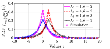
Figure 2: Validation for PDF of ${\log_{2}\left({\bar{\gamma}^{{}^{\mathcal{S}\mathcal{U}}}_{{}_{\mathcal{S}\mathcal{A}}}}\right)}$ with $D=r$ under eavesdropping.

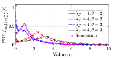
Figure 3: Validation for PDF of ${\log_{2}\left(1+{\bar{\gamma}^{{}^{\mathcal{S}\mathcal{U}}}_{{}_{\mathcal{A}\mathcal{U}}}}\right)}$ with $D=R$ under jamming.

Firstly, the expression (19) for PDF ${{f}}_{\log_{2}\left({\bar{\gamma}^{{}^{\mathcal{S}\mathcal{U}}}_{{}_{\mathcal{S}\mathcal{A}}}}\right)}\left(c\right)$ is validated in Fig. 2. It also represents the PDF of SC ${\hat{C}}^{\mathcal{E}}_{{}_{1,2}}$ for the cases 1 and 2 under eavesdropping mode under high SNR regime as observed from (29) provided ${\log_{2}\left({\bar{\gamma}^{{}^{\mathcal{S}\mathcal{U}}}_{{}_{\mathcal{S}\mathcal{A}}}}\right)\geq 0}$. Hence, it is represented as ${{f}}_{\hat{C}^{\mathcal{E}}_{{}_{1,2}}}\left(c\right)$ for further discussion. We have used $10^{6}$ random realisations of distances $d_{{}_{\mathcal{S}\mathcal{U}}}$ and $d_{{}_{\mathcal{S}\mathcal{A}}}$ to generate simulation results. Analytical and simulation results are found to be in close agreement with root mean square error (RMSE) $<10^{-4}$. Similarly, Fig. 3, validates the analytical expression for PDF ${f}_{\log_{2}\left(1+{\bar{\gamma}^{{}^{\mathcal{S}\mathcal{U}}}_{{}_{\mathcal{A}\mathcal{U}}}}\right)}\left(c\right)$ given by (21) which also represents PDF of SC ${\hat{C}^{\mathcal{J}}}$ under jamming mode in high SNR regime, as explained in (32). Therefore, equivalent representation of PDF can be expressed as ${{f}}_{\hat{C}^{\mathcal{J}}}\left(c\right)$. A close match is observed between analytical and simulation results with RMSE $<10^{-4}$. We have validated the PDFs ${{f}}_{\hat{C}^{\mathcal{E}}_{{}_{1,2}}}\left(c\right)$ and $f_{{\hat{C}}^{\mathcal{J}}}$ are for various values of ratio $\lambda_{\mathcal{E}}$, $\lambda_{\mathcal{J}}$ respectively and analysed the impact of path-loss exponent $\theta$ also. Here, $\lambda_{\mathcal{E}}$ reflects the ratio of channel parameters $a_{{}_{\mathcal{S}\mathcal{U}}}$ to $a_{{}_{\mathcal{S}\mathcal{A}}}$ and $\lambda_{\mathcal{J}}$ represents ratio of channel parameters $a_{{}_{\mathcal{S}\mathcal{U}}}$ to $a_{{}_{\mathcal{A}\mathcal{U}}}$ for $P_{{\mathcal{S}}}=P_{{\mathcal{J}}}$. The effect of relative channel conditions of legitimate and both attacker links are revealed in Figs. 2 and 3 Higher channel gain of legitimate link compared to that for legitimate link is found to yield larger realisations of ${\hat{C}}^{\mathcal{E}}_{{}_{1,2}}$ and ${\hat{C}}^{\mathcal{J}}$ in eavesdropping and jamming respectively. Larger spread in both distributions is also observed for a larger value of path-loss exponent $\theta$. Since asymptotic SOP $\hat{p}^{\mathcal{E}}_{o}$ and $\hat{p}^{\mathcal{J}}_{o}$ in $\eqref{eq:outage_E_Th2_highsnr}$ and $\eqref{eq:outage_J_Th3}$ respectively are functions of asymptotic SC, SOP analysis carried out in Section 4 is also verified by analytical validation of SC.

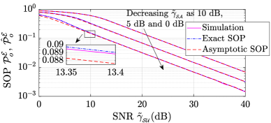
Figure 4: SOP validation for $R\!=\!r\!=\!D$ under eavesdropping.

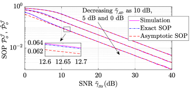
Figure 5: SOP validation $R=D$ under jamming.

Figs. 4 and 5 verify the accuracy of closed-form solutions given by (30) and (33) for SOPs derived through asymptotic analysis. They are compared with the exact SOPs given by (IV-A1) and (IV-A2) in Section 4 under eavesdropping and jamming modes respectively. Analytical results for the exact SOP are also compared with Monte-Carlo simulation results and found in close agreement. Fig. 4 shows variation of SOP ${p}^{\mathcal{E}}_{o}$ and asymptotic SOP $\hat{p}^{\mathcal{E}}_{o}$ against worst case SNRs as denoted by ${\tilde{\gamma}_{{}_{\mathcal{S}\mathcal{U}}}}$ and $\tilde{\gamma}_{{}_{\mathcal{S}\mathcal{A}}}$. Similarly, variation of SOPs ${p}^{\mathcal{J}}_{o}$ and asymptotic SOP $\hat{p}^{\mathcal{J}}_{o}$ are plotted in Fig. 5 against worst case SNRs ${\tilde{\gamma}_{{}_{\mathcal{S}\mathcal{U}}}}$ and $\tilde{\gamma}_{{}_{\mathcal{A}\mathcal{U}}}$. Hereby, $\tilde{\gamma}_{{}_{\mathcal{S}\mathcal{U}}}$ = $\frac{\kappa_{{}_{\mathcal{S}\mathcal{U}}}}{D^{\theta}}$, $\tilde{\gamma}_{{}_{\mathcal{S}\mathcal{A}}}$ = $\frac{\kappa_{{}_{\mathcal{S}\mathcal{A}}}}{r^{\theta}}$, and $\tilde{\gamma}_{{}_{\mathcal{A}\mathcal{U}}}$ = $\frac{\kappa_{{}_{\mathcal{A}\mathcal{U}}}}{R^{\theta}}$. For $\tilde{\gamma}_{{}_{\mathcal{S}\mathcal{A}}}=\tilde{\gamma}_{{}_{\mathcal{A}\mathcal{U}}}=0$ dB, we observe that results are closely matching for $\tilde{\gamma}_{{}_{\mathcal{S}\mathcal{D}}}>7$ dB under eavesdropping and $\tilde{\gamma}_{{}_{\mathcal{S}\mathcal{D}}}>9$ dB under jamming. It is also revealed that under the condition $\tilde{\gamma}_{{}_{\mathcal{S}\mathcal{A}}}=\tilde{\gamma}_{{}_{\mathcal{A}\mathcal{U}}}=5$ dB, results are in good agreement under eavesdropping while very low deviations are observed for $\tilde{\gamma}_{{}_{\mathcal{S}\mathcal{D}}}<5$ dB under jamming. Hence, closed-form results derived for asymptotic SOP holds good for evaluating SOP for wide range of practical values of SNR for legitimate as well as both attacker channels. Henceforth, we refer the asymptotic SOP as simply SOP.

VI-B Insight about design parameters

Figs. 6 to 9 deliver the valuable insights about deigning of system parameters for achieving intended secrecy performance in accordance with the discussion carried out in Section 5. The impact of maximum distance $D$ between legitimate nodes on SOP is analysed in Fig 6 with varying eavesdropping range $r$ of $\mathcal{A}$. Since $r$ and $D$ reflect the restriction on random inter-node distances respectively ${d_{{}_{\mathcal{S}\mathcal{A}}}}$ for effective eavesdropping and ${d_{{}_{\mathcal{S}\mathcal{U}}}}$ for maintaining QoS under eavesdropping as well as jamming, we may take extreme values of $r=r_{max}=R$ and $D=D_{max}=2R$ to represent a traditional scenario when no restriction is put on corresponding distances in terms of these variables. A significant rise in SOP $\hat{p}^{\mathcal{E}}_{o}$ is recorded for $D>D_{o}$. The results also reveal that $D$ influence SOP $\hat{p}^{\mathcal{E}}_{o}$ more adversely as compared to $r$. We also note that, satisfying the condition $r$ ¿ $r_{sat}$ results in constant SOP for $D\leq D_{o}$ where $r_{sat}$ is defined in Section 5. For a typical value of $D$= 60 m, SOP saturates to 0.11 for $r>r_{sat}=75$ m and becomes independent of a further increase in eavesdropping range. Fig. 6 also exhibits the uni-modal nature of $\hat{p}^{\mathcal{E}}_{o}$ in $r$. It shows that there exists a value of $r$ that gives optimal performance. This optimal value of $r$ can be utilised by $\mathcal{A}$ for posing maximum adverse impact on the secrecy performance of legitimate communication in an efficient manner as compared to its extreme value.

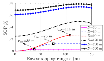
Figure 6: Insights about $r$ with $R\!=\!150$ m, $D_{o}\!=\!100$ m under eavesdropping.

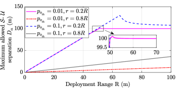
Figure 7: Maximum allowed $D$ under eavesdropping.

Remark 1.

The SOP $\hat{p}^{\mathcal{E}}_{o}$ under eavesdropping can be retained at a remarkably lower value by meeting the conditions $D\leq D_{o}$. Furthermore, from attacker point of view, eavesdropping range of $\mathcal{A}$ can be restricted to $r_{sat}$ instead of its extreme value for $D<D_{o}$ as no further gain is attained by $\mathcal{A}$ towards secrecy outage. Equivalently, $\mathcal{S}$-$\mathcal{U}$ pair can restrict the maximum separation between them to $D_{{}_{sat}}$ so as to neutralise the impact of eavesdropping range on $\hat{p}^{\mathcal{E}}_{o}$ beyond a given value of $r$ provided $D_{{}_{sat}}\leq D_{o}$. It may, therefore, be recognised that for technologies used for short-range communication like D2D and IoT, the effect of $r$ gets saturated beyond a certain value while an important role is played by $r$ in secrecy performance for technologies used for long range communications.

Fig. 7 provides the insights about $D_{{}_{{th}}}$, the maximum value of allowed $D$ to achieve an acceptable value of SOP ${{p}}_{o_{{}_{th}}}$ for various values of ${{p}}_{o_{{}_{th}}}$ and $r$ with varying $R$. It is observed that $D_{{}_{{th}}}$ exhibits increasing nature with ${{p}}_{o_{{}_{th}}}$ and decreasing trend with $r$. We also find that the value of $D_{{}_{{th}}}$ linearly increases with increased $R$ for $D_{{}_{{th}}}<D_{o}$ or $D_{{}_{{th}}}=D_{max}$. The former condition happens because of the fact that for $D_{{}_{{th}}}<D_{o}$, ${{p}}_{o_{{}_{th}}}$ is a function of $\frac{D_{{}_{{th}}}}{R}$. The latter condition is based on the fact that acceptable value of SOP ${{p}}_{o_{{}_{th}}}$ is high enough that maximum communication range can be enjoyed by legitimate nodes for $D_{{}_{{th}}}=D_{max}$ which is found to be a linear function of $R$. Under the former condition, when $D_{{}_{{th}}}$ exceeds $D_{o}$ with increasing $R$, the behaviour of $D_{{}_{{th}}}$ is illustrated for practical range of $\hat{{p}}_{o_{{}_{th}}}$ in Fig. 7. It is noticed that, $D_{{}_{{th}}}$ fastly decreases first to meet acceptable SOP ${{p}}_{o_{{}_{th}}}$ and then gradually decreases with $R$. This illustration, thus, can be used as a reference for the design of secrecy performance aware $D_{{}_{{th}}}$.

Remark 2.

Under eavesdropping, the large deployment range supports in the greater maximum allowed $\mathcal{S}-\mathcal{U}$ separation $D_{{}_{{th}}}$ for a given acceptable SOP ${{p}}_{o_{{}_{th}}}$ provided $D_{{}_{{th}}}<D_{o}$ or $D_{{}_{{th}}}=D_{max}$. For $D_{o}\leq D_{{}_{{th}}}<D_{max}$, there is no advantage in increasing $R$ further for the purpose of enhancing secrecy QoS aware $D_{{}_{{th}}}$ for a practical range of acceptable SOP.

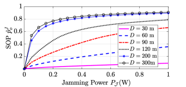
Figure 8: SOP under jamming for $R\!=\!150$ m, $D_{o}=100$ m.

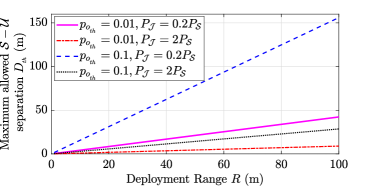
Figure 9: Maximum allowed $D$ under jamming.

In Fig. 8 we plot variation of SOP $\hat{p}^{\mathcal{J}}_{o}$ with $\mathcal{A}$’s jamming power $P_{\mathcal{J}}$ and maximum distance between legitimate nodes $D$. Results show that for $D\leq D_{o}$, $\hat{p}^{\mathcal{J}}_{o}$ increases almost linearly with increased $P_{\mathcal{J}}$. For $D>D_{o}$, there is a sharp increase in $\hat{p}^{\mathcal{J}}_{o}$. After a point, $\hat{p}^{\mathcal{J}}_{o}$ increases gradually and gets saturated with $P_{\mathcal{J}}$. For a particular value of $D>200$ m and $P_{\mathcal{J}}>0.5$ W, $\hat{p}^{\mathcal{J}}_{o}$ does not increase significantly and almost gets saturated at $P_{\mathcal{J}}>1.5$ W which implies that $\mathcal{A}$ gets diminished returns by increasing $P_{\mathcal{J}}$ beyond this. Moreover, the impact of $D$ is found more detrimental on $\hat{p}^{\mathcal{J}}_{o}$ relative to $P_{\mathcal{J}}.$

Remark 3.

The setting of $D\leq D_{o}$ enables us to retain a lower level of SOP $\hat{p}^{\mathcal{J}}_{o}$ in the presence of $\mathcal{A}$ in jamming mode. Though, degradation is significant for $D>D_{o}$, $\mathcal{A}$ gets diminishing returns by increasing $P_{\mathcal{J}}$ beyond a certain point. Therefore, in short-range communication technologies like D2D, jamming power plays a more important role in degrading secrecy performance. Whereas in long-range communication technologies, the role of jamming power diminishes after a certain point.

These observations reflect that proposed model aids to analyse secrecy performance in a better way as compared to the traditional scenario when real-life constraints in terms of distance thresholds are not considered. Then the maximum allowed $\mathcal{S}-\mathcal{U}$ separation ${D_{{}_{th}}}$, for the acceptable SOP ${{p}}_{o_{{}_{th}}}=0.01$ and $0.1$ are plotted with different values of $P_{\mathcal{J}}$ in Fig. 9 for jamming mode. It is observed that ${D_{{}_{th}}}$ increases linearly with $R$ for a given acceptable SOP ${{p}}_{o_{{}_{th}}}$ because ${{p}}_{o_{{}_{th}}}$ is a function of $\frac{D_{{}_{{th}}}}{R}$. This ${D_{{}_{th}}}$ is found as an increasing function of ${{p}}_{o_{{}_{th}}}$ and a decreasing function of $P_{\mathcal{J}}$. The impact of ${{p}}_{o_{{}_{th}}}$ on $D_{{}_{{th}}}$ gets reduced with increased $P_{\mathcal{J}}$.

Remark 4.

The larger deployment range results in large value of maximum allowed $\mathcal{S}-\mathcal{U}$ separation $D_{{}_{{th}}}$ for an acceptable SOP ${{p}}_{o_{{}_{th}}}$ under jamming.

To analyse the impact of randomness in channel fading gain on designing of $D_{th}$, we plot its PDF $f_{D_{th}}(x)$ against its values $x$ under eavesdropping and jamming in respectively Figs. 10 (a) and (b). We consider the random channel power gains due to Rayleigh fading with the same mean value as in Figs. 7 and 9. Channel fading gains $\left|h_{{}_{ij}}\right|^{2},\;\forall\;i,j=\left\{\mathcal{S},\mathcal{U},\mathcal{A}\right\}$ follow exponential distribution. We also find that, $D_{th}$ increases with an increased ratio of fading gains $\frac{|{h}_{{}_{\mathcal{S}\mathcal{U}}}|^{2}}{|{h}_{{}_{\mathcal{S}\mathcal{A}}}|^{2}}$ for eavesdropping and $\frac{|{h}_{{}_{\mathcal{S}\mathcal{U}}}|^{2}}{|{h}_{{}_{\mathcal{A}\mathcal{U}}}|^{2}}$ for jamming. This can be explained by the fact that SOP decreases with an increased ratio of channel gains $\frac{|\mathrm{g}_{{}_{\mathcal{S}\mathcal{U}}}|^{2}}{|\mathrm{g}_{{}_{\mathcal{S}\mathcal{A}}}|^{2}}$ and $\frac{|\mathrm{g}_{{}_{\mathcal{S}\mathcal{U}}}|^{2}}{|\mathrm{g}_{{}_{\mathcal{A}\mathcal{U}}}|^{2}}$ for eavesdropping and jamming respectively. Channel gains consist of a ratio of fading gain to the path loss, i.e., $\left|\mathrm{g}_{{}_{ij}}\right|^{2}=\frac{\left|h_{{}_{ij}}\right|^{2}}{\left(d_{{}_{ij}}\right)^{\theta}},\;\forall\;i,j=\left\{\mathcal{S},\mathcal{U},\mathcal{A}\right\}$ where ${d_{{}_{\mathcal{S}\mathcal{U}}}}\leq D,{d_{{}_{\mathcal{S}\mathcal{A}}}}\leq r,{d_{{}_{\mathcal{A}\mathcal{U}}}}\leq R$. Therefore, for a given acceptable SOP ${{p}}_{o_{{}_{th}}}$, an increase in fading gain ratio leads to an increase in acceptable value of path loss in $\mathcal{S}$-$\mathcal{U}$ link due to ${d_{{}_{\mathcal{S}\mathcal{U}}}}$ for the given parameters. This, in turn, increases the maximum allowed $\mathcal{S}$-$\mathcal{U}$ separation $D_{th}$. These findings lead to the corresponding pdf of $D_{th}$ as observed in Figs. 10 (a) and 10 (b).Increasing values of ${{p}}_{o_{{}_{th}}}$ shift the curve towards right in the sense that the larger realisations of $D_{th}$ become more likely and vice versa.

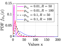
(a) Eavesdropping with $r$ = $0.8R$

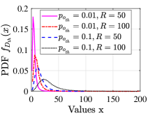
(b) Jamming with $P_{\mathcal{J}}=2P_{\mathcal{S}}$

Figure 10: Impact of channel fading randomness on $D_{th}$.

VI-C Relative Severity of Eavesdropping and Jamming

As discussed in Section 5, for a given secrecy rate threshold $C_{st}$ and channel parameters, there exists a corresponding threshold for distance threshold $D_{o}$ such that for $C_{st}\leq\log_{2}({1+\frac{\kappa_{{}_{{}_{\mathcal{S}\mathcal{U}}}}}{{D}^{\theta}}})$ or equivalently $D\leq D_{o}$, outage is caused by $\mathcal{A}$ only. For this scenario, under eavesdropping $p_{o}^{\mathcal{E}}$ initially increases with increased $r$ and saturates after reaching $\alpha=r^{2}/R^{2}$. For $C_{st}>\log_{2}({1+\frac{\kappa_{{}_{{}_{\mathcal{S}\mathcal{U}}}}}{{D}^{\theta}}})$ or equivalently $D>D_{o}$, there is a sharp increase in SOP caused by randomness in propagation losses along with security breach due to presence of $\mathcal{A}$ because there is no guarantee to support the high secrecy rate $C_{st}$ by legitimate link. SOPs $\hat{p}^{\mathcal{E}}_{o}$ and $\hat{p}^{\mathcal{J}}_{o}$ increases with $r$ and $P_{\mathcal{J}}$ in eavesdropping and jamming respectively.

We observe that under the same channel conditions for eavesdropping and jamming link, $\mathcal{A}$ in jamming mode with $P_{\mathcal{J}}<P_{\mathcal{S}}$ yields SOP $\hat{p}^{\mathcal{J}}_{o}$ less than $\hat{p}^{\mathcal{E}}_{o}$ in eavesdropping mode with $r=R$. Hence, under these conditions, $\mathcal{A}$ prefers eavesdropping relative to jamming to cause the maximum secrecy outage to the legitimate nodes. However, for $r<R$, jammer becomes more harmful than eavesdropper beyond a definite $C_{st}$.

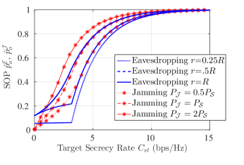
Figure 11: Variation in SOP under eavesdropping and jamming with $R=100$ m, $D=50$ m.

This condition is true for both cases: with $P_{\mathcal{J}}<P_{\mathcal{S}}$ and $P_{\mathcal{J}}\geq P_{\mathcal{S}}$. At a very low value of $C_{st}$ (near to zero), SOP is higher under eavesdropping because there may be a probability of zero SC which includes the probability of negative secrecy capacity as defined by (4), whereas there is always positive SC under jamming.

Remark 5.

By maintaining $D\leq D_{o}$, SOP $\hat{p}^{\mathcal{E}}_{o}$ in eavesdropping can be limited to $\alpha=r^{2}/R^{2}$. Furthermore, eavesdropping has more severe impact on secrecy performance than jamming for the same channel conditions for eavesdropping and jamming link unless $r<R$ or $P_{\mathcal{S}}<P_{\mathcal{J}}$.

VII Concluding Remarks

This paper proposes a novel QoS-aware stochastic system model and investigates the impact of random inter-node distances under eavesdropping as well as jamming. Development of ratio distribution of legitimate to attacker link SNR for the proposed system in closed-form makes an important and significant contribution in the knowledge domain. This has enabled us to derive novel closed-form expressions for SOP. Analytical expressions have been validated against simulation results with almost perfect match. New insights are drawn for designing of system parameters in order to achieve the desired SOP. The proposed model has been shown to design maximum $\mathcal{S}$-$\mathcal{U}$ separation for achieving desired secrecy performance. From attacker point of view, it is shown through numerical results that an optimal value of eavesdropping range can be designed to cause maximum secrecy outage. It is also shown that no gain is achieved by $\mathcal{A}$ beyond a threshold value of eavesdropping range for given conditions. In the case of jamming, $\mathcal{A}$ gets a diminishing returns beyond a threshold value of jamming power. Also, the conditions are discussed under which there is a linear increment in the maximum allowed separation between legitimate nodes with increased deployment range for an acceptable SOP. Finally, we compare the severity of eavesdropping and jamming in terms of secrecy outage. It is observed that for the same set of channel conditions for $\mathcal{S}$-$\mathcal{A}$ and $\mathcal{A}$-$\mathcal{U}$ links, $\mathcal{A}$ must have more transmit power than $\mathcal{S}$ to pose more secrecy outage in jamming than eavesdropping provided that it is capable to eavesdrop in entire deployment range. It is, therefore, established that the proposed analytical model offers a reference framework for inferring deep insights into functioning of eavesdropping and jamming. It can also be leveraged as an analytical design tool for determining system parameters to achieve the required secrecy performance.

References

- [1] B. Ahuja, D. Mishra, and R. Bose, “Novel QoS-aware physical layer security analysis,” in Proc. IEEE ICC, Shanghai, China, May 2019, pp. 1–6.
- [2] A. Mukherjee, “Physical-layer security in the Internet of Things: Sensing and communication confidentiality under resource constraints,” Proc. IEEE, vol. 103, no. 10, pp. 1747–1761, Oct. 2015.
- [3] R. Zhang, X. Cheng, and L. Yang, “Cooperation via spectrum sharing for physical layer security in Device-to-Device communications underlaying cellular networks,” IEEE Trans. Wireless Commun., vol. 15, no. 8, pp. 5651–5663, Aug. 2016.
- [4] R. Zhang, L. Song, Z. Han, and B. Jiao, “Physical layer security for two-way untrusted relaying with friendly jammers,” IEEE Trans. Veh. Technol., vol. 61, no. 8, pp. 3693–3704, Oct. 2012.
- [5] B. Li, Y. Zou, J. Zhou, F. Wang, W. Cao, and Y. Yao, “Secrecy outage probability analysis of friendly jammer selection aided multiuser scheduling for wireless networks,” IEEE Trans. Commun., vol. 67, no. 5, pp. 3482–3495, May 2019.
- [6] ——, “Secrecy outage probability analysis of friendly jammer selection aided multiuser scheduling for wireless networks,” IEEE Trans. Commun., vol. 67, no. 5, pp. 3482–3495, May 2019.
- [7] Y. Zou, “Physical-layer security for spectrum sharing systems,” IEEE Trans. Wireless Commun., vol. 16, no. 2, pp. 1319–1329, Feb. 2017.
- [8] X. Liu, “Outage probability of secrecy capacity over correlated log-normal fading channels,” IEEE Commun. Lett., vol. 17, no. 2, pp. 289–292, Feb. 2013.
- [9] L. Lv, Z. Ding, Q. Ni, and J. Chen, “Secure MISO-NOMA transmission with artificial noise,” IEEE Trans. Veh. Technol., vol. 67, no. 7, pp. 6700–6705, July 2018.
- [10] N. S. Ferdinand, D. B. da Costa, and M. Latva-aho, “Effects of outdated CSI on the secrecy performance of MISO wiretap channels with transmit antenna selection,” IEEE Commun. Lett., vol. 17, no. 5, pp. 864–867, May 2013.
- [11] X. Li, J. Li, and L. Li, “Performance analysis of impaired SWIPT NOMA relaying networks over imperfect Weibull channels,” IEEE Syst. J., pp. 1–4, 2019, early access.
- [12] P. C. Pinto, J. Barros, and M. Z. Win, “Physical-layer security in stochastic wireless networks,” in Proc. IEEE Int. Conf. Commun. (ICC), Guangzhou, China, Nov. 2008, pp. 974–979.
- [13] ——, “Secure communication in stochastic wireless networks part I: Connectivity,” IEEE Trans. Inf. Forensics Security, vol. 7, no. 1, pp. 125–138, Feb. 2012.
- [14] W. Liu, Z. Ding, T. Ratnarajah, and J. Xue, “On ergodic secrecy capacity of random wireless networks with protected zones,” IEEE Trans. Veh. Technol., vol. 65, no. 8, pp. 6146–6158, Aug. 2016.
- [15] M. A. Kishk and H. S. Dhillon, “Coexistence of RF-powered IoT and a primary wireless network with secrecy guard zones,” IEEE Trans. Wireless Commun., vol. 17, no. 3, pp. 1460–1473, Mar. 2018.
- [16] S. Srinivasa and M. Haenggi, “Distance distributions in finite uniformly random networks: Theory and applications,” IEEE Trans. Veh. Technol., vol. 59, no. 2, pp. 940–949, Feb. 2010.
- [17] F. Tong and J. Pan, “Random-to-random nodal distance distributions in finite wireless networks,” IEEE Trans. Veh. Technol., vol. 66, no. 11, pp. 10 070–10 083, Nov. 2017.
- [18] F. Tong, Y. Wan, L. Zheng, J. Pan, and L. Cai, “A probabilistic distance-based modeling and analysis for cellular networks with underlaying device-to-device communications,” IEEE Trans. Wireless Commun., vol. 16, no. 1, pp. 451–463, Jan. 2017.
- [19] G. T. Amariucai and S. Wei, “Half-duplex active eavesdropping in fast-fading channels: A block-markov wyner secrecy encoding scheme,” IEEE Trans. Inf. Theory, vol. 58, no. 7, pp. 4660–4677, Jul. 2012.
- [20] A. Garnaev, M. Baykal-Gursoy, and H. V. Poor, “A game theoretic analysis of secret and reliable communication with active and passive adversarial modes,” IEEE Trans. Wireless Commun., vol. 15, no. 3, pp. 2155–2163, Mar. 2016.
- [21] B. Ahuja, D. Mishra, and R. Bose, “Optimal green hybrid attacks in secure IoT,” IEEE Wireless Commun. Lett., pp. 1–1, 2019, early access.
- [22] L. Lv, Z. Ding, J. Chen, and N. Al-Dhahir, “Design of secure NOMA against full-duplex proactive eavesdropping,” IEEE Wireless Commun. Lett., vol. 8, no. 4, pp. 1090–1094, Aug. 2019.
- [23] B. Ahuja, D. Mishra, and R. Bose, “Fairness-aware subcarrier allocation to combat full duplex eavesdropping and jamming attacks in IoT,” in Proc. IEEE ICC, Dublin, Ireland, 2020, pp. 1–6, accepted.
- [24] H. Chen, X. Tao, N. Li, Y. Hou, J. Xu, and Z. Han, “Secrecy performance analysis for hybrid wiretapping systems using random matrix theory,” IEEE Trans. Wireless Commun., vol. 18, no. 2, pp. 1101–1114, Feb. 2019.
- [25] H. Masoumi and M. J. Emadi, “Performance analysis of cell-free massive MIMO system with limited fronthaul capacity and hardware impairments,” IEEE Trans. Wireless Commun., pp. 1–1, 2019, early access.
- [26] X. Li, J. Li, Y. Liu, Z. Ding, and A. Nallanathan, “Residual transceiver hardware impairments on cooperative NOMA networks,” IEEE Trans. Wireless Commun., pp. 1–1, 2019, early access.
- [27] X. Li, M. Liu, C. Deng, P. T. Mathiopoulos, Z. Ding, and Y. Liu, “Full-duplex cooperative NOMA relaying systems with I/Q imbalance and imperfect SIC,” IEEE Wireless Commun. Lett., pp. 1–1, 2019, early access.
- [28] E. Ahmed and A. M. Eltawil, “On phase noise suppression in full-duplex systems,” IEEE Trans. Wireless Commun., vol. 14, no. 3, pp. 1237–1251, Mar. 2015.
- [29] A. Goldsmith, Wireless Communications, 1st ed. Cambridge University Press, 2004.
- [30] A. D. Wyner, “The wire-tap channel,” The Bell System Technical Journal, vol. 54, no. 8, pp. 1355–1387, Oct. 1975.
- [31] Q. Zhu, W. Saad, Z. Han, H. V. Poor, and T. BaÅŸar, “Eavesdropping and jamming in next-generation wireless networks: A game-theoretic approach,” in Proc. IEEE Military Commun. Conf. (MILCOM), Baltimore, USA, Nov. 2011, pp. 119–124.
- [32] J. Y. Ryu, J. Lee, and T. Q. S. Quek, “Transmission strategy against opportunistic attack for MISO secure channels,” IEEE Commun. Lett., vol. 20, no. 11, pp. 2304–2307, Nov. 2016.
- [33] S.-J. Tu and E. Fischbach, A New Geometric Probability Technique for an N-Dimensional Sphere and Its Applications, math-ph/0004021 ed. arxiv.org, 2000, vol. arXiv preprint.
- [34] E. W. Weisstein, “Incomplete Beta Function,” accessed Sep. 25, 2018, http://bias.csr.unibo.it/fvc2002/databases.asp.
- [35] P. Omiyi, H. Haas, and G. Auer, “Analysis of TDD cellular interference mitigation using busy-bursts,” IEEE Trans. Wireless Commun., vol. 6, no. 7, pp. 2721–2731, Jul. 2007.
- [36] A. Papoulis and S. U. Pillai, Probability, Random Variables, and Stochastic Processes, 4th ed. McGraw-Hill Higher Education, 2002.
- [37] M. Bloch, J. Barros, M. R. D. Rodrigues, and S. W. McLaughlin, “Wireless information-theoretic security,” IEEE Trans. Inf. Theory, vol. 54, no. 6, pp. 2515–2534, June 2008.
- [38] I. R. I.S. Gradshteyn, Table of Integrals, series and products, 7th ed. Elseveir, 2007.
- [39] R. Rezaei, S. Sun, X. Kang, Y. L. Guan, and M. R. Pakravan, “Secrecy throughput maximization for full-duplex wireless powered IoT networks under fairness constraints,” IEEE Internet Things J., vol. 6, no. 4, pp. 6964–6976, Aug. 2019.
- [40] M. Andersson, “Short range low power wireless devices and Internet of Things (IoT),” U-Blox, Tech. Report,, Tech. Rep., 2015.