Statistical Approach to Detection of Attacks for Stochastic Cyber-Physical Systems

Abstract

We study the problem of detecting an attack on a stochastic cyber-physical system. We aim to treat the problem in its most general form. We start by introducing the notion of asymptotically detectable attacks, as those attacks introducing changes to the system’s output statistics which persist asymptotically. We then provide a necessary and sufficient condition for asymptotic detectability. This condition preserves generality as it holds under no restrictive assumption on the system and attacking scheme. To show the importance of this condition, we apply it to detect certain attacking schemes which are undetectable using simple statistics. Our necessary and sufficient condition naturally leads to an algorithm which gives a confidence level for attack detection. We present simulation results to illustrate the performance of this algorithm.

I Introduction

A Cyber-physical systems (CPS) is a physical system which is monitored or controlled via a communication channel. It finds a wide range of applications such as traffic signal systems [1], health care [2], energy manufacturing [3], power system [4, 5, 6, 7, 8], the water industry [9, 10]. A CPS is prone to attacks in the form of signals injected through the communication link [2]. These attacks are known to have caused a number of serious accidents around the world [11, 12, 13, 14, 15]. They have generated urgency for detecting such attacks.

In principle, an attack may be regarded as a system fault. This permits using methods for fault tolerant control, such as robust statistics [16], robust control [17] and failure detection and identification [18]. However, the essential difference between an attack and a fault is that the design of the former aims at making it difficult for detection. For example, Liu et al studied how to inject a stealthy input into the measurement without being detected by the classical failure detector [19]. Hence, methods for CPS attack detection need to take special care of this difference.

Early works on CPS attack detection rely on certain prior knowledge of the attacker’s model. Among these methods, we find: The work in [20], deals with a kind of attack called denial of service. The works [19] and [21] concentrate on false data injection attacks against state estimation. The authors of [22] introduced stealthy deception attacks, which consist in manipulating the measurements to be processed by a power system state estimator in such a manner that the resulting systematic errors introduced by the adversary are either undetected or only partially detected by a bad data detection method. In [23], the effect of replay attacks is studied. Smith investigated the behavior of control systems under covert attacks [24], where a malicious agent can access the signals and information within the control loop and use them to disrupt or compromise the controlled plant.

It is often unrealistic to assume that the defender has some knowledge of the attacker’s model. To address this concern, recent works have studied the CPS attack problem without an attacking model assumption. In this line, Pasqualetti et al studied the problem of detectability, by describing the undetectable/unidentificable attack class, consisting of attacks not detectable by any kind of detection method [25]. Using this concept, they studied in [25, 26] the design of centralized and distributed attack detection methods. However, this approach is limited to systems without process and measurement noises. The study of systems involving random noises is much more challenging, since these systems present more ambiguities where attacks can be hidden.

Concerning the detection of attacks in systems with noise, Mo and Sinopoli [27] analyzed the estimation error introduced by an attack which is not detected by a $\chi^{2}$ failure detector. They also studied in [28] the attacks on scalar systems with multiple sensors. In [29], the authors introduce the notion of strictly stealthy and $\epsilon$-stealthy attacks, and bound the performance deterioration achievable by such attacks.

In this work we move a step forward in the research line described above. As in [27, 28, 29], we also study systems with noise. We start by introducing the notion of asymptotically stealthy attacks, as an extension of the definition of strict stealthiness given in [29], to the case where the system and attack are non-stationary. More precisely, strict stealthiness means that the attack does not change the output statistics. Therefore, it cannot be detected by any method using statistical knowledge of the system’s output. However, if the detector only knows a single realization of the system’s output, this definition is too restrictive. We relax this condition, by defining an attack to be asymptotically stealthy if the changes it induces on output statistics vanish asymptotically. We then define an attack to be asymptotically detectable if it is not asymptotically stealthy. Some rigorous statistical setup is required to make our definition precise.

To make the notion of asymptotic detectability verifiable, we provide a necessary and sufficient condition for it. This condition is expressed in terms of certain statistical properties, which are in principle testable using the knowledge of a single realization. The condition is given without requiring any assumption on the attacking model, and, under mild regularity conditions, is valid for the general case in which the system being attacked is time-varying, non-linear and with non-Gaussian noises. We also specialize this condition for the case of stationary linear system with Gaussian noises.

To appreciate the importance of the introduced notion of asymptotic detectability and the provided necessary and sufficient condition, we give two examples of attacks, which cannot be detected by checking commonly used statistics, but are instead detected by checking our condition.

In view of our main result, testing that an attack is detectable requires verifying a condition which is numerically intractable. To fill this gap, we derive a practically feasible detection algorithm. While we do so for the case in which the system is linear and Gaussian, the algorithm can be readily extended to arbitrary non-linear non-Gaussian systems. Also, while the class of attacks that can be detected by this algorithm is smaller than the class of asymptotically detectable attacks, the difference between these two classes can be made arbitrarily small by sufficiently increasing the complexity of the algorithm.

The rest of this paper is organized as follows. In Section II we introduce the required statistical background. In Section III we describe the attack detection problem. In Section IV we introduce the definition of asymptotically detectable attacks. In Section V we give a necessary and sufficient condition for asymptotic detectability. More precisely, in Section V-A we treat the general case, and in Section V-B we specialize this result for the case of stationary linear system with Gaussian noises. In Section VI, we discuss attack examples which cannot be detected by checking other simpler conditions. In Section VII we use our condition to derive the detection algorithm. In Section VIII we use simulations to illustrate the superiority of our algorithm for detecting attacks that cannot be detected by other simpler methods. Finally, concluding remarks are stated in Section IX.

II Preliminaries

Notation 1.

We use $\mathbb{N}$ to denote the set of natural numbers, $\mathbb{Z}$ to denote the set of integers, $\mathbb{R}_{+}$ to denote the set of non-negative real numbers and $\bar{\mathbb{R}}=\mathbb{R}\cup\{-\infty,\infty\}$ to denote the set of extended real numbers. For a vector $x$ we use $\left[x\right]_{i}$ to denote its $i$-th entry and for a matrix $X$ we use $\left[X\right]_{i,j}$ to denote its $(i,j)$-th entry. For a vector or matrix $X$, we use $X^{\top}$ to denote its transpose. For vectors $x$ and $y$, $x\prec y$ ($x\preceq y$) means that $\left[x\right]_{i}<\left[y\right]_{i}$ ($\left[x\right]_{i}\leq\left[y\right]_{i}$), for all $i$, and $z=x\wedge y$ denotes the vector with entries $[z]_{i}=\min(x_{i},y_{i})$. We use $\mathbf{1}$ to denote a column vector of ones, $\mathbf{I}$ to denote the identity matrix, $q$ to denote the forward-shift operator, i.e., $(qx)_{t}=x_{t+1}$, and $\mathds{1}_{S}$ to denote the indicator function of the set $s$, i.e., $\mathds{1}_{S}(x)=1$, if $x\in S$ and $0$ otherwise. We also use $\phi_{\mu,\Sigma}$ and $\Phi_{\mu,\Sigma}$ to denote the probability density function (PDF) and cumulative distribution function (CDF), respectively, of the normal distribution with mean $\mu$ and covariance matrix $\Sigma$.

Notation 2.

Let $\mathbb{S}^{D}=\left(\mathbb{R}^{D}\right)^{\mathbb{N}}$ denote the set of all sequences $x=\left(x_{t}\in\mathbb{R}^{D}:t\in\mathbb{N}\right)$ indexed by the natural numbers. Let $\mathcal{\mathcal{S}}^{D}$ denote the sigma algebra on $\mathbb{S}^{D}$ generated by the cylinder sets

$$C_{t}\left(A\right) = \left\{x\in\mathbb{S}^{D}:x_{t}\in A\right\},\quad\text{for all }t\in\mathbb{N},A\subseteq\mathbb{R}^{D}.$$

Definition 1.

Let $\left(\Omega,\mathcal{A},\mathbb{P}\right)$ denote a probability space. A $D$-dimensional random process is a map $x:\Omega\rightarrow\mathbb{S}^{D}$, measurable with respect to $\mathcal{A}$ and $\mathcal{S}^{D}$. Its probability distribution $p$ is

$$p\left(x\in S\right)=\mathbb{P}\circ x^{-1}\left(S\right)\text{ for all }S\in\mathcal{S}^{D}.$$

A random process $x$ is said to be asymptotically mean stationary (AMS) [30, S 7.3] if

$$\lim_{T\rightarrow\infty}\frac{1}{T}\sum_{t=1}^{T}p\left(q^{t}x\in S\right)\text{ exists for all }S\in\mathcal{S}^{D}.$$

In this case, the associated stationary probability distribution $\bar{p}$ is defined by

$$\bar{p}\left(x\in S\right)=\lim_{T\rightarrow\infty}\frac{1}{T}\sum_{t=1}^{T}p\left(q^{t}x\in S\right)\text{ for all }S\in\mathcal{S}^{D}.$$ (1)

For a measurable map $f:\mathbb{S}^{D}\rightarrow\mathbb{R}$, we define its stationary mean by

$$\bar{\mathcal{E}}\left\{f(x)\right\}=\int f(x)d\bar{p}.$$

Also, $x$ is said to be ergodic [30, S 7.7] if, for all $S\in\mathcal{S}^{D}$,

$$qS=S\Rightarrow p\left(qx\right)=0\text{ or }1.$$

AMS and ergodicity are properties which are stated in a rather technical way. Roughly speaking, the AMS property is required for all limits of sample averages to exist w.p.1. Also, ergodicity is required for these limit values to be equal w.p.1. These statements are made precise by the AMS ergodic theorem [30, Th. 8.1].

III Problem description

We have the following system in state-space form

$$x_{t+1} =f_{t}\left(x_{t},w_{t}\right),$$ (2)

$$y_{t} =g_{t}\left(x_{t},v_{t}\right),$$ (3)

where $f_{t}:\mathbb{R}^{D_{x}}\times\mathbb{R}^{D_{w}}\rightarrow\mathbb{R}^{D_{x}}$ and $g_{t}:\mathbb{R}^{D_{x}}\times\mathbb{R}^{D_{v}}\rightarrow\mathbb{R}^{D}$ are (measurable) non-linear time-varying functions, and the process noise $w_{t}$, $t\in\mathbb{Z}$, and measurement noise $v_{t}$, $t\in\mathbb{Z}$, are sequences of random vectors. We assume that $y$ is AMS, ergodic, and its distribution $p\left(y\in S\right)$, $S\in\mathcal{S}^{D}$ is absolutely continuous.

Consider an attacker, which interferes the measurement signal $y_{t}$, replaces it with an attacking signal $z_{t}$, and sends $z_{t}$ instead of $y_{t}$ to the receiver. In order to treat the problem in its full generality, we assume that $z_{t}$ is generated by an arbitrary (possibly non-linear and non-stationary) measurable function of the whole history of $y_{s}$ up to time $t$, i.e.,

$$z_{t}=h_{t}\left(y_{s}:t\geq s\in\mathbb{N}\right).$$

Problem 1.

The attack detection problem consists in assessing whether or not $z=y$.

Definition 2.

We say that the statistics of a random variable/process are nominal if they equal those which occur when $z=y$. The probability law and expected value taken with respect to these statistics are denoted by $p_{\star}\left(\cdot\right)$ and $\mathcal{E}_{\star}\left\{\cdot\right\}$, respectively.

IV Asymptotic detectability

In order to assess whether $z=y$, all the information that we have is a single realization of $z$ and the probability distribution of $y$, i.e., $p(y\in S)$, for all $S\in\mathcal{S}^{D}$. The latter equals the nominal probability distribution $p_{\star}(z\in S)$ of $z$, i.e., when there is no attack. In [29], under the assumption that $y$ is stationary, an attack was defined to be (strictly) stealthy if it satisfies a condition which is equivalent to

$$p\left(z\in S\right)=p_{\star}\left(z\in S\right)\text{ for all }S\in\mathcal{S}.$$ (4)

In the case in which $y$ is non-stationary, since we only know a single realization of $z$, it is impossible to check (4). However, we can still hope to check whether the stationary distribution of $z$ (cf. (1)) matches its nominal value, provided both exist. This leads to our definition of asymptotic stealthiness and asymptotic detectability listed below, which do not require the existence of either stationary distribution.

Definition 3.

We say that $z$ is asymptotically stealthy if

$$\lim_{T\rightarrow\infty}\frac{1}{T}\sum_{t=1}^{T}\left[p\left(q^{t}z\in S\right)-p_{\star}\left(q^{t}z\in S\right)\right]=0\text{ for all }S\in\mathcal{S}.$$ (5)

Otherwise, we say that $z$ is asymptotically detectable.

Remark 1.

An attack is asymptotically detectable if it causes a modification in the probability distribution $p\left(q^{t}z\in S\right)$ which is persistent over time. Hence, in particular, every finite-time attack is asymptotically stealthy. Asymptotic detectability essentially means that it is possible to detect the presence of the attack, with a confidence that tends to one as the number of observed samples tends to infinity. Obviously, in a practical setting, any method aiming at approximating the Cesàro summation in (5) will be carried out over a sliding time window of finite length. This permits detecting finite-time attacks with a confidence that depends on the window length and the duration of the attack. We derive one such methods in Section VII, and discus the choice of the sliding window length in Remark 4.

V A necessary and sufficient condition for asymptotic detectability

Our definition of asymptotic detectability is obviously impractical, because it requires considering all possible test functions which are integrable under the nominal distribution. In this section we provide a necessary and sufficient condition for asymptotic detectability. In Section V-A we do so for the general case described in Section III, and in Section V-B we specialize this result for the case in which the system (2)-(3) is stationary, linear, and with Gaussian noises.

V-A The general case

Let $L\in\mathbb{N}$, $\zeta_{t}^{(L)}=\left[z_{t}^{\top},\cdots,z_{t+L-1}^{\top}\right]^{\top}$ and $\rho\in\mathbb{R}^{LD}$. Let also

$$F_{\star}^{(L)}(\rho)=\bar{p}_{\star}\left(\zeta_{1}^{(L)}\preceq\rho\right),$$ (6)

be the nominal CDF of $\zeta_{1}^{(L)}$. For each $T\in\mathbb{N}$, let

$$F_{T}^{(L)}\left(\rho\right)=\frac{1}{T}\sum_{t=1}^{T}\mathds{1}_{\left\{\zeta_{t}^{(L)}\preceq\rho\right\}}(\rho),$$ (7)

be a sample approximation of the true stationary CDF $F^{(L)}(\rho)=\bar{p}\left(\zeta_{1}^{(L)}\preceq\rho\right)$. The next theorem uses these definitions to provide a necessary and sufficient condition for asymptotic stealthiness.

Theorem 1.

If $y$ is AMS, ergodic and its distribution is absolutely continuous, the process $z$ is asymptotically stealthy if and only if, for all $L\in\mathbb{N}$ and $\rho\in\mathbb{R}^{LD}$,

$$\lim_{T\rightarrow\infty}F_{T}^{(L)}\left(\rho\right)\overset{\text{w.p.1}}{=}F_{\star}^{(L)}(\rho).$$ (8)

We devote the rest of the section to the proof of Theorem 1.

Notation 3.

For $x,y\in\mathbb{S}^{D}$, we define the distance

$$d\left(x,y\right)=\sum_{t=1}^{\infty}2^{-t}\left(1\wedge\left|x_{t}-y_{t}\right|\right).$$

As shown in [31, p. 241], under the topology induced by $d$, $\mathbb{S}^{D}$ is separable and complete. For a set $S\in\mathcal{S}^{D}$, we use $\bar{S}$ to denote its closure under this topology. Also, we use $\partial S=\bar{S}\cap\overline{\left(\mathbb{S}^{D}\setminus S\right)}$ to denote the boundary of $S$.

For $L,T\in\mathbb{N}$, and $S\in\mathcal{S}^{D}$, let the measure $\bar{p}_{T}\left(z\in\cdot\right):\mathcal{S}^{D}\rightarrow\mathbb{R}_{+}$ be defined by

$$\bar{p}_{T}\left(z\in S\right)=\frac{1}{T}\sum_{t=1}^{T}p\left(q^{t}z\in S\right).$$

For $L\in\mathbb{N}$ and $\rho\in\bar{\mathbb{R}}^{LD}$, let $R_{\rho}^{L}\in\mathcal{\mathcal{S}}^{D}$ be the set

$$R_{\rho}^{L}=\left\{x\in\mathbb{S}^{D}:\left[x_{1}^{\top},\cdots,x_{L}^{\top}\right]^{\top}\preceq\rho\right\}.$$

Lemma 1.

If $y$ is AMS and its distribution is absolutely continuous, then $\bar{p}_{\star}\left(\check{z}\in\partial S\right)=0$, for any $S\in\mathcal{S}^{D}$.

Proof:

We split the proof in steps:

Step 1) Let $\mathcal{R}=\left\{R_{\rho}^{L}:L\in\mathbb{N},\rho\in\bar{\mathbb{R}}^{LD}\right\}$. Let $L,M\in\mathbb{N}$, $\rho\in\bar{\mathbb{R}}^{LD}$ and $\lambda\in\bar{\mathbb{R}}^{MD}$. Without loss of generality, suppose that $M\geq L$, and let $\tilde{\rho}=\left[\rho^{\top},\infty,\cdots,\infty\right]^{\top}$ be padded so that $\tilde{\rho}\in\bar{\mathbb{R}}^{MD}$. We have

$$R_{\rho}^{L}\cap R_{\lambda}^{M}=R_{\tilde{\rho}}^{M}\cap R_{\lambda}^{M}=R_{\tilde{\rho}\wedge\lambda}^{M}.$$

Hence, $\mathcal{R}$ is a $\pi$-system [32, Def. 1.1].

Step 2) Let $\mathcal{M}$ denote the collection of sets $M\subseteq\mathbb{S}^{D}$ such that $\bar{p}_{\star}\left(\check{z}\in\partial M\right)=0$. We have that

$$\bar{p}_{\star}\left(\check{z}\in\partial\mathbb{S}^{D}\right)=\bar{p}_{\star}\left(\check{z}\in\emptyset\right)=0.$$

Also, if $M\subset N\in\mathcal{M}$,

$$\bar{p}_{\star}\left(\check{z}\in\partial\left(N\setminus M\right)\right) =\bar{p}_{\star}\left(\check{z}\in\partial N\cup\partial M\right)$$

$$\leq\bar{p}_{\star}\left(\check{z}\in\partial N\right)+\bar{p}_{\star}\left(\check{z}\in\partial M\right)=0,$$

and, if $M_{k}\in\mathcal{M}$, $k\in\mathbb{N}$, are disjoint, and $M=\bigcup_{k\in\mathbb{N}}M_{k}$, then,

$$\bar{p}_{\star}\left(\check{z}\in\partial\left(M\right)\right)\leq\sum_{k\in\mathbb{N}}\bar{p}_{\star}\left(\check{z}\in\partial M_{k}\right)=0.$$

Hence, $\mathcal{M}$ is a $\lambda$-system [32, Def. 1.10].

Step 3) Let $\delta\left(\mathcal{R}\right)$ be the smallest $\lambda$-system containing $\mathcal{R}$. Since the distribution of $y$ is absolutely continuous, then clearly so is its stationary distribution $\bar{p}\left(y\in S\right)$. Hence, since the latter equals $\bar{p}_{\star}\left(z\in S\right)$, we have $\mathcal{R}\subseteq\mathcal{M}$ and $\mathcal{M}$ is a $\lambda$-system, then $\delta\left(\mathcal{R}\right)\subseteq\mathcal{M}$. Thus, from Dynkin’s $\pi$-$\lambda$ theorem [32, Th. 1.19], $\delta\left(\mathcal{R}\right)=\sigma\left(\mathcal{R}\right)$. But from [32, Th. 1.23] and the definition of $\mathcal{S}^{D}$, $\sigma\left(\mathcal{R}\right)=\mathcal{S}^{D}$. So we have that $\mathcal{S}^{D}\subseteq\mathcal{M}$ and the result follows. ∎

Lemma 2.

If $y$ is AMS, its distribution is absolutely continuous and (8) holds, then $z$ is AMS and for all $S\in\mathcal{S}^{D}$,

$$\bar{p}\left(z\in S\right)=\bar{p}_{\star}\left(z\in S\right).$$ (9)

Proof:

Let $t_{k}\in\mathbb{N}$, for $k=1,\cdots,K$, and $\tau=\left[t_{1},\cdots,t_{K}\right]^{\top}$. Let also $\lambda_{k}\in\bar{\mathbb{R}}^{D}$, for $k=1,\cdots,K$, and $\lambda=\left[\lambda_{1}^{\top},\cdots,\lambda_{K}^{\top}\right]^{\top}$. Consider the set $D_{\lambda}^{\tau}\in\mathcal{S}^{D}$ defined by

$$D_{\lambda}^{\tau}=\left\{x\in\mathbb{S}^{D}:x_{t_{k}}\preceq\lambda\right\}.$$

We have that $D_{\lambda}^{\tau}=R_{\rho}^{L}$, where $L=t_{k}$ and $\rho=\left[\rho_{1}^{\top},\cdots,\rho_{L}^{\top}\right]^{\top}$ with $\rho_{l}=\lambda_{l}$ if $l=t_{k}$ and $\infty\mathbf{1}$ otherwise. We then have that, for all $\tau$ and $\lambda$,

$$\lim_{T\rightarrow\infty}\bar{p}_{T}\left(z\in D_{\lambda}^{\tau}\right)=\lim_{T\rightarrow\infty}\frac{1}{T}\sum_{t=1}^{T}\mathcal{E}\left\{\mathds{1}_{\left\{\zeta_{t}^{(L)}\preceq\rho\right\}}\left(\rho\right)\right\}\overset{\text{(a)}}{=}\mathcal{E}\left\{\lim_{T\rightarrow\infty}F_{T}^{(L)}\left(\rho\right)\right\}\overset{\text{(b)}}{=}F_{\star}^{(L)}(\rho)=\bar{p}_{\star}\left(z\in D_{\lambda}^{\tau}\right),$$

where (a) follows from Lebesgue’s dominated convergence theorem and (b) follows from (8). It then follows from [31, Example 2.4] that the sequence of probability measures $\bar{p}_{T}\left(z\in\cdot\right):\mathcal{S}^{D}\rightarrow\mathbb{R}_{+}$ converges weakly to $\bar{p}_{\star}\left(z\in\cdot\right)$, i.e., for all $f\in C_{b}\left(\mathbb{S}^{D}\right)$ (the space of continuous bounded functions on $\mathbb{S}^{D}$),

$$\lim_{T\rightarrow\infty}\int fd\bar{p}_{T}=\int fd\bar{p}_{\star}.$$

It the follows from [31, Th. 2.1], that, for each $S\in\mathcal{S}^{D}$, with $\bar{p}_{\star}\left(z\in\partial S\right)=0$,

$$\lim_{T\rightarrow\infty}\bar{p}_{T}\left(z\in S\right)=\bar{p}_{\star}\left(z\in S\right).$$

Then, (9) follows from the above since, in view of Lemma 1, $\bar{p}_{\star}\left(z\in\partial S\right)=0$ holds for all $S\in\mathcal{S}^{D}$. ∎

Proof:

Only if part: If $z$ is asymptotically stealthy, since $y$ is AMS, then clearly also is $z$. Also, since $\bar{p}_{\star}\left(z\in S\right)=\bar{p}\left(y\in S\right)$, for all $S\in\mathcal{S}^{D}$, and $y$ is AMS and ergodic, it follows from [30, Lemma 7.13] that $z$ is ergodic. Then, from the AMS ergodic theorem [30, Th. 8.1],

$$\lim_{T\rightarrow\infty}F_{T}^{(L)}(\rho)\overset{\text{w.p.1}}{=}\bar{\mathcal{E}}_{\star}\left\{\mathds{1}_{R_{\rho}^{L}}\left(z\right)\right\}=F_{\star}^{(L)}(\rho),$$

and (8) holds.

If part: If (8) holds, since $y$ is AMS, the asymptotic stealthiness of $z$ follows immediately from Lemma 2. ∎

V-B The stationary linear Gaussian case

In this subsection we specialize the result of Theorem 1 for the case in which (2)-(3) have the following form

$$x_{t+1} =Ax_{t}+w_{t},$$

$$y_{t} =Cx_{t}+v_{t},$$

with $w_{t}\sim\mathcal{N}\left(0,Q\right)$ and $v_{t}\sim\mathcal{N}\left(0,R\right)$. We also assume that the system is in steady state, i.e., $x_{t}\sim\mathcal{N}\left(0,P\right)$, with $P=APA^{\top}+Q$.

If we run a Kalman filter, in steady state we obtain

$$\hat{x}_{t+1|t} =A\hat{x}_{t|t-1}+K\left(z_{t}-C\hat{x}_{t|t-1}\right),$$ (10)

$$K =A\Psi C^{\top}\left(C\Psi C^{\top}+R\right)^{-1},$$

where $\Psi$ is the solution of

$$\Psi=A\Psi A^{\top}-A\Psi C^{\top}\left(C\Psi C^{\top}+R\right)^{-1}C\Psi A^{\top}+Q.$$

Let $\hat{z}_{t|t-1}=C\hat{x}_{t|t-1}$, $\tilde{z}_{t}=z_{t}-\hat{z}_{t|t-1}$ and $\Gamma=C\Psi C^{\top}+R$. Let also

$$\check{z}_{t}=\Gamma^{-1/2}\tilde{z}_{t}.$$ (11)

Under nominal statistics, we have that $\Gamma$ is the covariance of $\tilde{z}_{t}$. Thus, since the samples of $\tilde{z}$ are independent, those of $\check{z}$ are independent and identically distributed (i.i.d.), with $\check{z}_{t}\sim\mathcal{N}(0,\mathbf{I})$. In view of this, it would be numerically more convenient if the condition of Theorem 1 could be given in terms of $\check{z}$. This is done in the next corollary of Theorem 1. Let $\check{F}_{T}^{(L)}$ be defined as in (7), but with $\check{z}$ in place of $z$.

Corollary 1.

The process $z$ is asymptotically stealthy if and only if, for all $L\in\mathbb{N}$ and $\rho\in\mathbb{R}^{LD}$,

$$\lim_{T\rightarrow\infty}\check{F}_{T}^{(L)}\left(\rho\right)\overset{\text{w.p.1}}{=}\Phi_{0,\mathbf{I}}(\rho).$$ (12)

Proof:

We split the proof in steps:

Step 1) Clearly, if the statistics of $z$ are nominal, then so are those of $\check{z}$ (i.e., it is i.i.d. with $\check{z}_{t}\sim\mathcal{N}(0,\mathbf{I})$). The converse also holds since $z_{t}$ is fully determined by $\left(\check{z}_{s}:t\geq s\in\mathbb{Z}\right)$, via the recursions

$$\hat{x}_{t+1|t}=A\hat{x}_{t|t-1}+K\Gamma^{1/2}\check{z}_{t},\qquad z_{t}=C\hat{x}_{t|t-1}+\Gamma^{1/2}\check{z}_{t}.$$

It is then straightforward to check that $\bar{p}\left(z\in S\right)=\bar{p}_{\star}\left(z\in S\right)$ if and only if $\bar{p}\left(\check{z}\in S\right)=\bar{p}_{\star}\left(\check{z}\in S\right)$. Hence, asserting that $z$ has nominal stationary statistics is equivalent to asserting that $\check{z}$ also has.

Step 2) Since $y$ is AMS, $z$ has nominal stationary statistics if and only if it is asymptotically stealthy. The same conclusion can be drawn for $\check{z}$. Then, combining these two facts with the conclusion from Step 1), we obtain that $z$ is asymptotically stealthy if and only if $\check{z}$ is so.

Step 3) Let $\check{y}$ be defined as $\check{z}$ but using $y$ in place of $z$. Clearly, $\check{y}$ satisfies the conditions of $y$ in Theorem 1. It then follows from this theorem that $\check{z}$ is asymptotically stealthy if and only if (12) holds. The result then follows from the conclusion of Step 2). ∎

Remark 2.

The family of tests (12) can be understood as a normality test. More precisely, as checking the following condition

$$\check{z}_{t}\text{ is }\mathcal{N}(0,\mathbf{I})\text{ and i.i.d}.$$ (13)

Corollary 1 asserts that this test enjoys the property of being equivalent of the asymptotic stealthiness of the process $z$. However, notice that not every normality test run on the sequence $\check{z}_{t}$ may enjoy this property, and therefore usable for assessing asymptotic stealthiness.

VI Attack examples whose detection requires Theorem 1

Checking the condition of Corollary 1 essentially means checking that the stationary probability distribution $\bar{p}$ of $\check{z}$ equals the nominal one $\bar{p}_{\star}$, i.e., that under the distribution $\bar{p}$, (13) holds. As it is known, from a theoretical point of view, checking that a block of samples has joint standard normal distribution is a stronger requirement than doing some other more practical checks, e.g., for pairwise independence or uncorrelation. However, the question arise as to whether, for the purposes of detecting an attack, it is really necessary to carry out a full distribution check, or if instead, a simpler test would be enough. In this section we provide two examples showing how an asymptotically detectable attack can pass undetected if a test checking only for uncorrelation or pairwise independence is used. This supports our claim that checking the condition of Theorem 1 is indeed needed.

VI-A Checking for uncorrelation

By combining a normality test [33], together with a test for uncorrelation [34, §14.2], we can verify the following condition

$$\check{z}_{t}\sim\mathcal{N}\left(0,\mathbf{I}\right)\text{ and $\bar{\mathcal{E}}$}_{\star}\left\{\check{z}_{t}\check{z}_{s}^{\top}\right\}=0,\forall t\neq s\in\mathbb{N}.$$ (14)

However, condition (13) is stronger that (14), in the sense that the former requires that $\check{z}_{t}$ and $\check{z}_{s}$ are statistically independent, rather than uncorrelated, when $t\neq s$. In this section we describe an attack example which can be detected by a method verifying (13), but not by one verifying (14).

Suppose that we feed the output $y$ to the Kalman filter (10). Let $\check{y}_{t}\sim\mathcal{N}\left(0,\mathbf{I}\right)$ denote the resulting normalized prediction error, obtained as in (11). Let $\tau\in\mathbb{N}$, $0<\upsilon<1$ and $\gamma_{t}$ be an i.i.d. sequence of binary random variables with $p\left(\gamma_{t}=0\right)=p\left(\gamma_{t}=1\right)=0.5$. Let $r_{0}\sim\mathcal{N}\left(0,\mathbf{I}\right)$ and

$$r_{t} = \upsilon r_{t-\tau}+\sqrt{1-\upsilon^{2}}\check{y}_{t},\qquad\check{z}_{t}=\gamma_{t}r_{t}.$$ (15)

Since $\check{y}_{t}\sim\mathcal{N}\left(0,\mathbf{I}\right)$ is i.i.d., it is straightforward to see that $r_{t}\sim\mathcal{N}\left(0,\mathbf{I}\right)$. Hence $\check{z}_{t}\sim\mathcal{N}\left(0,\mathbf{I}\right)$. Also, if $t\neq s$,

$$\mathcal{E}\left\{\check{z}_{t}\check{z}_{s}^{\top}\right\}=\left(1-\upsilon^{2}\right)\mathcal{E}\left\{\gamma_{t}\right\}\mathcal{E}\left\{\gamma_{s}\right\}\mathcal{E}\left\{r_{t}r_{s}\right\}=0.$$

Hence, the process $\check{z}$ satisfies (14). However, since

$$\check{z}_{t}=\gamma_{t}\left(\upsilon r_{t-\tau}+\sqrt{1-\upsilon^{2}}\check{y}_{t}\right),\quad\check{z}_{t-\tau}=\gamma_{t-\tau}r_{t-\tau},$$

the vector $\left[\check{z}_{t}^{\top},\check{z}_{t-\tau}^{\top}\right]^{\top}$ is clearly not Gaussian. Hence, $\check{z}$ does not satisfy (13). Since the attacker knows $y_{s}$, for all $s\leq t$, it can always build the attacking signal $z_{t}$ such that the normalized prediction error $\check{z}$ at the receiver equals the one described above. Such an attack can be detected by (13) but not by (14).

VI-B Checking for pairwise independence

A combination of a normality test [33] with a test for pairwise independence [34, §15], [35] permit checking the following condition

$$\left[\check{z}_{t}^{\top}\check{z}_{s}^{\top}\right]^{\top}\sim\mathcal{N}\left(0,\mathbf{I}\right),\forall t\neq s.$$ (16)

As it is known, assessing that (13) holds is not equivalent to assessing (16). This is because pairwise independence does not imply joint independence in general. We describe below an attacking scheme which would be detected by (13), but not by (16).

Let the measurement dimension $D=1$. As before, we feed the output $y$ to the Kalman filter (10), and let $\check{y}_{t}\sim\mathcal{N}\left(0,1\right)$ denote the normalized prediction error. Draw $\left[\check{z}_{0},\check{z}_{-1}\right]$ from the distribution $\mathcal{N}(0,\mathbf{I})$. Then, for $t\in\mathbb{N}$, we compute

$$\check{z}_{t}=\begin{cases}\check{y}_{t},&t\text{ even},\\ \mathrm{sign}\left(\check{z}_{t-1}\check{z}_{t-2}\right)\left|\check{y}_{t}\right|,&t\text{ odd}.\end{cases}$$ (17)

We first analyze pairwise independence. If $t$ is even $\check{z}_{t}$ is obviously independent of $\check{z}_{s}$, for all $s\neq t$. So we assume that $t$ is odd. Suppose that at time $t$, the vector $\left[\check{z}_{t-1},\check{z}_{t-2}\right]$ has distribution $\mathcal{N}\left(0,\mathbf{I}\right)$. We have

$$p\left(\check{z}_{t},\check{z}_{t-1}\right)=p\left(\check{z}_{t}|\check{z}_{t-1}\right)p\left(\check{z}_{t-1}\right).$$

Now

$$p\left(\check{z}_{t}=\beta|\check{z}_{t-1}\right)=\begin{cases}\frac{1}{2}p\left(\left|\check{y}_{t}\right|=\beta\right),&\beta>0\\ \frac{1}{2}p\left(-\left|\check{y}_{t}\right|=\beta\right),&\beta\leq 0\end{cases}=\phi_{0,1}\left(\beta\right).$$

Also, $\check{z}_{t-1}\sim\mathcal{N}(0,1)$. Hence $\left[\check{z}_{t},\check{z}_{t-1}\right]\sim\mathcal{N}\left(0,\mathbf{I}\right)$. By symmetry, we also have that $\left[\check{z}_{t},\check{z}_{t-2}\right]\sim\mathcal{N}\left(0,\mathbf{I}\right)$. Since clearly $\left[\check{z}_{t},\check{z}_{s}\right]\sim\mathcal{N}\left(0,\mathbf{I}\right)$ for any even $s$, it remains to be shown that $\left[\check{z}_{t},\check{z}_{2s+1}\right]\sim\mathcal{N}\left(0,\mathbf{I}\right)$, for all $s$. This follows immediately from (17), since $\check{z}_{t-2}$ is independent of $\check{z}_{2s+1}$. Then, by induction on $t$, we have that (17) holds for all $t$ and $s$.

Now, clearly, if $t$ is even, $\left[\check{z}_{t},\check{z}_{t-1},\check{z}_{t-2}\right]\sim\mathcal{N}\left(0,\mathbf{I}\right)$, However, for any odd $t$, $\check{z}_{t}\check{z}_{t-1}\check{z}_{t-2}\geq 0$. Then,

$$\left[\check{z}_{t},\check{z}_{t-1},\check{z}_{t-2}\right]\nsim\mathcal{N}\left(0,\mathbf{I}\right).$$ (18)

Hence, while $\check{z}$ is clearly AMS, in view of (18), it does not satisfy (13). We can then draw the same conclusions as those in Section VI-A.

VII Attack detection algorithm

An attack detection algorithm cannot be readily obtained from Theorem 1 or Corollary 1. This is because this result requires carrying out the uncountable family of tests (8). Moreover, each of these tests requires an infinite number of attacked samples. Hence, they cannot detect sporadic attacks that last a finite time interval. Nevertheless, numerically tractable algorithms can be readily derived using these results. In this section we derive one such algorithm, for the case of linear systems with Gaussian noises, based on the result from Corollary 1. More precisely, we propose a test which, for each time step, produces a single statistic which summarizes the outcome of a finite number of tests (8). A similar algorithm for detecting attacks in a general non-linear system can be derived from the conditions of Theorem 1.

In order to cope with the fact that the family of tests (8) is uncountable, we first point out that it is enough to consider the largest $L$ that the available computational resources allow. Then, for this fixed value of $L$, we define a set of sample points on $\mathbb{R}^{LD}$ at which we will test condition (8). We use $\rho_{i}=\left[\rho_{i,0}^{\top},\cdots,\rho_{i,L-1}^{\top}\right]^{\top}$, $i=1,\cdots,I$, to denote these points, with $\rho_{i,l}\in\mathbb{R}^{D}$, $l=0,\cdots,L-1$. Also, in order to go around the limitation that the tests (8) can not detect sporadic attacks, while in Corollary 1 $\check{F}_{T}^{(L)}$ is computed starting from time $1$, we use a moving horizon of $T$ time samples. Hence, for each sample time $t$ we define the block of samples $\check{\zeta}_{t}^{(L)}=\left[\check{z}_{t}^{\top},\cdots,\check{z}_{t+L-1}^{\top}\right]^{\top}$ within this horizon, and build its empirical CDF

$$\check{F}_{t,T}^{(L)}\left(\rho\right) =\frac{1}{T}\sum_{s=t-T+1}^{t}\mathds{1}_{\left\{\check{\zeta}_{s}^{(L)}\preceq\rho\right\}}(\rho).$$ (19)

We then sample $\check{F}_{t,T}^{(L)}$ and $\Phi_{0,\mathbf{I}}$ at the points $\rho_{i}$, $i=1,\cdots,I$, forming the vectors $u_{t,T}\in\mathbb{R}^{I}$ and $u_{\star}\in\mathbb{R}^{I}$, respectively, defined by

$$\left[u_{t,T}\right]_{i} =\check{F}_{t,T}^{(L)}\left(\rho_{i}\right),\quad\text{and}\quad\left[u_{\star}\right]_{i}=\Phi_{0,\mathbf{I}}\left(\rho_{i}\right).$$ (20)

We next define the following weighted difference between the above vectors

$$v_{t,T}=T\left(u_{t,T}-u_{\star}\right)^{\top}\Sigma^{-1}\left(u_{t,T}-u_{\star}\right),$$

where $\Sigma=\sum_{\tau\in\mathbb{Z}}\Sigma(\tau)$, with

$$\Sigma(\tau)=\bar{\mathcal{E}}_{\star}\left\{\left(\xi_{\tau}-u_{\star}\right)\left(\xi_{0}-u_{\star}\right)^{\top}\right\},$$

and $\xi_{t}\in\mathbb{R}^{I}$ given by

$$\left[\xi_{t}\right]_{i}=\mathds{1}_{\left\{\check{\zeta}_{t}^{(L)}\preceq\rho_{i}\right\}}\left(\rho_{i}\right)$$

We then have the following result.

In the proof of Proposition 1 requires Lemma 3, which is a generalization of the central limit theorem to the case of finite independent vector processes.

Definition 4.

A random process $x$ is $M$-independent if $x_{t}$ and $x_{s}$ are independent whenever $t-s>M$. It is called finite-independent if it is $M$-independent for some $M\in\mathbb{N}$.

Lemma 3.

Let $x$ be a stationary finite-independent vector random process with $\mathcal{E}\left\{\left\|x_{0}\right\|^{12}\right\}<\infty$. Let $\bar{x}=\mathcal{E}\left\{x_{0}\right\}$, $\Sigma(\tau)=\mathcal{E}\left\{\left(x_{\tau}-\bar{x}\right)\left(x_{0}-\bar{x}\right)^{\top}\right\}$ and $\Sigma=\sum_{\tau\in\mathbb{Z}}\Sigma(\tau)$. Let also

$$\hat{x}_{T}=\frac{1}{T}\sum_{t=1}^{T}x_{t}.$$ (21)

Then

$$\lim_{T\rightarrow\infty}\sqrt{T}\left(\hat{x}_{T}-\bar{x}\right)\overset{\mathcal{D}}{=}\mathcal{N}\left(0,\Sigma\right).$$

Proof:

The scalar version of the result is a simplified version of [36, Th. 27.4]. The vector version follows by applying Cramér-Wold theorem [36, Th. 29.4] to the scalar version. ∎

Proposition 1.

Under nominal statistics,

$$\lim_{T\rightarrow\infty}v_{t,T}\overset{\mathcal{D}}{=}\chi^{2}\left(I\right),\text{ for all }t\in\mathbb{Z},$$

where $\chi^{2}\left(I\right)$ is a chi-squared distribution with $I$ degrees of freedom.

Proof:

We can write $u_{t,T}$ and $u_{\star}$ as

$$u_{t,T}=\frac{1}{T}\sum_{s=t-T+1}^{t}\xi_{t},\quad\text{and}\quad u_{\star}=\bar{\mathcal{E}}_{\star}\left\{\xi_{0}\right\}.$$

Let $w_{t,T}=\sqrt{T}\Sigma^{-1/2}\left(u_{t,T}-u_{\star}\right)$. It follows from (19) that, under nominal statistics, the sequence $\left(\xi_{t}:t\in\mathbb{N}\right)$ is $(L-1)$-independent (i.e., $\xi_{t}$ and $\xi_{s}$ are independent whenever $t-s>L-1$). Hence, in view of Lemma 3

$$\lim_{T\rightarrow\infty}w_{t,T}\overset{\mathcal{D}}{=}\mathcal{N}\left(0,\mathbf{I}\right).$$ (22)

Now $v_{t,T}$ can be written as

$$v_{t,T}=\left\|w_{t,T}\right\|_{2}^{2}=\sum_{i=1}^{I}\left[w_{t,T}\right]_{i}^{2}.$$ (23)

Then, the result follows from (22) and the continuous mapping theorem [36, Corollary 1 of Th. 25.7]. ∎

Let $H_{I}$ denote the CDF of a chi-squared distribution with $I$ degrees of freedom. We define the confidence $\psi_{t,T}$ of rejecting the null hypothesis (i.e., of asserting that there is an attack) at time $t$ by

$$\psi_{t,T}=H_{I}\left(v_{t,T}\right).$$ (24)

In view of Proposition 1, $\psi_{t,T}$ is uniformly distributed on $[0,1]$. Hence, for a given alarm triggering threshold $0\leq\alpha\leq 1$ on $\psi_{t,T}$, the false alarm rate $\pi_{t,T}$ at time $t$ (i.e., the probability of triggering an alarm when there is no attack), is given by

$$\pi_{t,T}=p\left(\psi_{t,T}\geq\alpha\right)=1-\alpha.$$

In order to compute $\psi_{t,T}$ we need expressions for $\xi_{t}$, $u_{\star}$ and $\Sigma$. These are given in the next proposition.

Proposition 2.

For each $i,j=1,\cdots,I$, we have

$$\left[\xi_{t}\right]_{i} =\prod_{l=0}^{L-1}\mathds{1}_{\left\{\check{z}_{t+l}\preceq\rho_{i,l}\right\}},\;\text{and}\;\left[u_{\star}\right]_{i}=\prod_{l=0}^{L-1}\Phi_{0,\mathbf{I}}\left(\rho_{i,l}\right).$$ (25)

Also,

$$\Sigma=\sum_{t=-L+1}^{L-1}\Sigma(t),$$ (26)

where

$$\Sigma(t)=\tilde{\Sigma}(t)-\bar{\Sigma},$$ (27)

with

$$\left[\bar{\Sigma}\right]_{i,j}=\prod_{\tau=0}^{L-1}\Phi_{0,\mathbf{I}}\left(\rho_{i,\tau}\right)\Phi_{0,\mathbf{I}}\left(\rho_{j,\tau}\right),$$ (28)

and

$$\left[\tilde{\Sigma}(t)\right]_{i,j}=\begin{cases}\prod_{\tau=0}^{-t-1}\Phi_{0,\mathbf{I}}\left(\rho_{i,\tau}\right)\Phi_{0,\mathbf{I}}\left(\rho_{j,L+t+\tau}\right)\prod_{\tau=0}^{L+t-1}\Phi_{0,\mathbf{I}}\left(\rho_{i,\tau-t}\wedge\rho_{j,\tau}\right),&-L+1\leq t<0,\\ \prod_{\tau=0}^{L-1}\Phi_{0,\mathbf{I}}\left(\rho_{i,\tau}\wedge\rho_{j,\tau}\right),&t=0,\\ \prod_{\tau=0}^{t-1}\Phi_{0,\mathbf{I}}\left(\rho_{i,L-t+\tau}\right)\Phi_{0,\mathbf{I}}\left(\rho_{j,\tau}\right)\prod_{\tau=0}^{L-t-1}\Phi_{0,\mathbf{I}}\left(\rho_{i,\tau}\wedge\rho_{j,t+\tau}\right),&0<t\leq L-1.\end{cases}$$ (29)

Proof:

Equation (25) follows straightforwardly from (20). To show (29), recall that $\rho_{i}=\left[\rho_{i,0}^{\top},\rho_{i,1}^{\top},\ldots,\rho_{i,L-1}^{\top}\right]^{\top}$, $i=1,\cdots,I$, are vectors on $\mathbb{R}^{LD}$. For all $i=1,\cdots,I$,

$$\left[\xi_{t}\right]_{i}=\prod_{l=0}^{L-1}\mathds{1}_{\left\{\check{z}_{t+l}\preceq\rho_{i,l}\right\}},\quad\text{and}\quad\left[u_{\star}\right]_{i}=\prod_{l=0}^{L-1}\Phi_{0,\mathbf{I}}\left(\rho_{i,l}\right).$$

Then, for all $i,j=1,\cdots,I$, and $t\in\mathbb{Z}$,

$$\left[\Sigma(t)\right]_{i,j}=\left[\tilde{\Sigma}(t)\right]_{i,j}-\left[\bar{\Sigma}\right]_{i,j},$$ (30)

with

$$\left[\tilde{\Sigma}(t)\right]_{i,j} =\bar{\mathcal{E}}_{\star}\left\{\prod_{l=0}^{L-1}\mathds{1}_{\left\{\check{z}_{t+l}\preceq\rho_{i,l}\right\}}\mathds{1}_{\left\{\check{z}_{l}\preceq\rho_{j,l}\right\}}\right\},$$

$$\left[\bar{\Sigma}\right]_{i,j} =\prod_{l=0}^{L-1}\Phi_{0,\mathbf{I}}\left(\rho_{i,l}\right)\Phi_{0,\mathbf{I}}\left(\rho_{j,l}\right).$$

Suppose that $t\geq 0$. We have

$$\left[\tilde{\Sigma}(t)\right]_{i,j} =\bar{\mathcal{E}}_{\star}\left\{\prod_{\tau=0}^{t-1}\mathds{1}_{\left\{\check{z}_{\tau}\preceq\rho_{j,\tau}\right\}}\prod_{\tau=0}^{L-t-1}\mathds{1}_{\left\{\check{z}_{t+\tau}\preceq\rho_{i,\tau}\right\}}\mathds{1}_{\left\{\check{z}_{t+\tau}\preceq\rho_{j,t+\tau}\right\}}\prod_{\tau=0}^{t-1}\mathds{1}_{\left\{\check{z}_{L+\tau}\preceq\rho_{i,L-t+\tau}\right\}}\right\}$$

$$=\prod_{\tau=0}^{t-1}\Phi_{0,\mathbf{I}}\left(\rho_{i,L-t+\tau}\right)\Phi_{0,\mathbf{I}}\left(\rho_{j,\tau}\right)\prod_{\tau=0}^{L-t-1}\Phi_{0,\mathbf{I}}\left(\rho_{i,\tau}\wedge\rho_{j,t+\tau}\right).$$ (31)

and

$$\left[\bar{\Sigma}\right]_{i,j}=\prod_{\tau=0}^{t-1}\Phi_{0,\mathbf{I}}\left(\rho_{i,L-t+\tau}\right)\Phi_{0,\mathbf{I}}\left(\rho_{j,\tau}\right)\prod_{\tau=0}^{L-t-1}\Phi_{0,\mathbf{I}}\left(\rho_{i,\tau}\right)\Phi_{0,\mathbf{I}}\left(\rho_{j,t+\tau}\right).$$

Then, subtracting and factor out the common term we get

$$\left[\Sigma(t)\right]_{i,j}=\left[\prod_{\tau=0}^{t-1}\Phi_{0,\mathbf{I}}\left(\rho_{i,L-t+\tau}\right)\Phi_{0,\mathbf{I}}\left(\rho_{j,\tau}\right)\right]\left[\prod_{\tau=0}^{L-t-1}\Phi_{0,\mathbf{I}}\left(\rho_{i,\tau}\wedge\rho_{j,t+\tau}\right)-\prod_{\tau=0}^{L-t-1}\Phi_{0,\mathbf{I}}\left(\rho_{i,\tau}\right)\Phi_{0,\mathbf{I}}\left(\rho_{j,t+\tau}\right)\right].$$

The above equation shows that $\left[\Sigma(t)\right]_{i,j}=0$ for all $t\geq L$.

In the above equations we considered the case $t\geq 0$. This means that the samples $\check{z}_{t},\cdots,\check{z}_{t+L-1}$ associated with index $i$ are right-shifted with respect to those $\check{z}_{0},\cdots,\check{z}_{L-1}$ associated with index $j$. If we now consider the case $t\leq 0$ (both cases coincide when $t=0$), the samples associated with $j$ will be right-shifted with respect to those of $i$. Since the process $\check{z}$ is stationary, the equations will be the same as those above but swapping the indexes $i$ and $j$ and taking $-t$ instead of $t$. Hence we get

$$\left[\tilde{\Sigma}(t)\right]_{i,j}=\prod_{\tau=0}^{-t-1}\Phi_{0,\mathbf{I}}\left(\rho_{i,\tau}\right)\Phi_{0,\mathbf{I}}\left(\rho_{j,L+t+\tau}\right)\prod_{\tau=0}^{L+t-1}\Phi_{0,\mathbf{I}}\left(\rho_{i,\tau-t}\wedge\rho_{j,\tau}\right),$$ (32)

and

$$\left[\Sigma(t)\right]_{i,j}=\left[\prod_{\tau=0}^{-t-1}\Phi_{0,\mathbf{I}}\left(\rho_{i,\tau}\right)\Phi_{0,\mathbf{I}}\left(\rho_{j,L+t+\tau}\right)\right]\left[\prod_{\tau=0}^{L+t-1}\Phi_{0,\mathbf{I}}\left(\rho_{i,\tau-t}\wedge\rho_{j,\tau}\right)-\prod_{\tau=0}^{L+t-1}\Phi_{0,\mathbf{I}}\left(\rho_{i,\tau-t}\right)\Phi_{0,\mathbf{I}}\left(\rho_{j,\tau}\right)\right],$$

which shows that $\left[\Sigma(t)\right]_{i,j}=0$ for all $t\leq-L$. Hence (26) follows. Equations (27) and (28) follows from (30). And (29) follows from (31) and (32). ∎

The proposed method assesses the presence of an attack by measuring the squared distance between the nominal and empirical CDFs of $\check{\zeta}_{1}^{(L)}$. Since the domain of these functions is $\mathbb{R}^{LD}$, their distance is measured over the grid sample points $\rho_{i}\in\mathbb{R}^{LD}$, $i=1,\cdots,I$. In order to complete the description of the method, we need a criterion for choosing these points. To this end, we apply the generalized Lloyd’s algorithm [37, S 11.3] to the nominal probability distribution of $\check{\zeta}_{1}^{(L)}$, i.e., $\mathcal{N}\left(0,\mathbf{I}\right)$. We then obtain the algorithm summarized in Algorithm 1.

Initialization: choose $T,L,I\in\mathbb{N}$ and a threshold $\alpha>0$.

1. Run Lloyd’s algorithm on the $LD$-dimensional distribution $\mathcal{N}\left(0,\mathbf{I}\right)$, to obtain $\rho_{i}\in\mathbb{R}^{LD}$, $i=1,\cdots,I$.

2. Using the points $\rho_{i}$, $i=1,\cdots,I$, compute $u_{\star}$ and $\Sigma$.

Main loop: at time $t$, let $\tau=t-L+1$ and run the following steps.

1. Run the Kalman filter (10) to obtain $\hat{z}_{t|t-1}$.

2. Compute $\check{z}_{t}$ using (11).

3. Compute $\check{\zeta}_{\tau}^{(L)}$ using $\check{z}_{\tau},\cdots,\check{z}_{t}$.

4. Compute $u_{t,T}$ using $\check{\zeta}_{\tau-T+1}^{(L)},\cdots,\check{\zeta}_{\tau}^{(L)}$.

5. Using $u_{t,T}$ compute $v_{t,T}$.

6. Compute $\psi_{t,T}$ using $v_{t,T}$ and (24).

7. Trigger an alarm if $\psi_{t,T}\geq\alpha$.

Algorithm 1 Attack detection test

Remark 3.

Algorithm 1 is an approximation of the family of tests (12). The key property of this algorithm is that this approximation can be made arbitrarily accurate by increasing the values of $T$, $L$ and $I$.

Remark 4.

Concerning the choice of the time horizon $T$, while a large value increases the accuracy and therefore the sensitivity of the detector to the presence of an attack, it also decreases the detection speed, i.e., the time that the detector takes to react to the occurrence of an attack. Hence, in a practical implementation, $T$ need to be chosen to accommodate a trade off between sensitivity and speed. It is also possible to achieve a combination of high detection speed to strong attacks and high sensitivity for detecting subtle attacks with slow detection speed, by running in parallel two instances of the same method, one with a small time horizon and the other with a large one.

VIII Simulation

In this section we illustrate our proposed method. Since this method checks that the joint statistics (JS) of a block of contiguous samples equal their nominal values, we refer to it as JS. We compare the JS method with other two. The first one is the method described in Section VI-B, which checks for the normality as well as pairwise independence (NPI) of samples of $\check{z}$. To do so, the method compares the joint CDFs of the vector $\left[\check{z}_{t}^{\top},\check{z}_{t-l}^{\top}\right]^{\top}$, for all values $l=1,\cdots,L-1$, using a procedure similar to the one described in Section VII. This yields the $L-1$ statistics $v_{t,T}^{(l)}$, $l=1,\cdots,L-1$, which are computed as in (23). We refer to this method as NPI. The second method is the one described in [27, eqs. (6)-(7)]. This method checks that the second order (SO) statistics of samples of the prediction error $\tilde{z}$ equal their nominal values. In our notation, it defines

$$v_{t,T}=\tilde{z}_{t}^{\top}\Gamma\tilde{z}_{t}\sim\chi^{2}\left(D\right).$$

We refer to this method as SO.

To do the comparison, we use a system with $A=0.98$, $C=1$, $R=0.1$ and $Q=0.1.$ Also, for the JS and NPI methods we use $I=100$, $L=3$ and $T=100$.

In the first experiment we consider the attack described in (15), with $\tau=1$ and $\alpha=1/\sqrt{2}$. As described in Section VI-A, this attack introduces statistical dependence between samples of $\check{z}$ which are $\tau$ samples away from each other. However, these samples remain uncorrelated. The left sides of Figures 1, 2 and 3 show the values of the statistic $v_{t,T}$ for the methods JS, NPI and SO, respectively. We see how the SO method is unable to detect the appearance of the attack at time $t=25\times 10^{3}$.

In the second experiment, we consider the attack described in (17). As explained in that section, this attack introduces statistical dependence between three consecutive samples of $\check{z}$, while leaving all samples from $\check{z}$ being pairwise independent. The values of $v_{t,T}$ for the methods JS, NPI and SO, are shown at the right sides of Figures 1, 2 and 3, respectively. We see that in this case, only the JS method is able to detect the appearance of the attack.

Remark 5.

As stated in Corollary 1, checking (12), for arbitrarily large $L$ and all $\rho$, guarantees the detection of all asymptotically detectable attacks. However, recall that algorithm JS only checks (12) for a fixed $L$ and a finite number of points $\rho_{i}\in\mathbb{R}^{LD}$, $i=1,\cdots,I$. Hence, certain asymptotically detectable attacks can escape the detection of algorithm JS. While the set of escaping attacks can be made arbitrarily small by increasing $L$ and $I$, there exists always the possibility that some attack can escape algorithm JS but not other algorithm like SO.

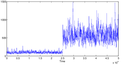
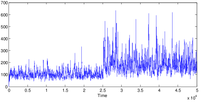
Figure 1: Evolution of $v_{t,T}$ yield by the JS detection method under attack (15) (left) and attack (17) (right).

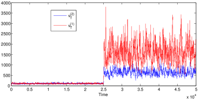
Figure 2: Evolution of $v_{t,T}^{(1)}$ and $v_{t,T}^{(2)}$ yield by the NPI detection method under attack (15) (left) and attack (17) (right).

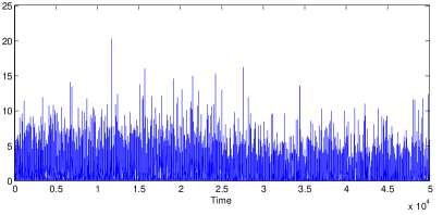
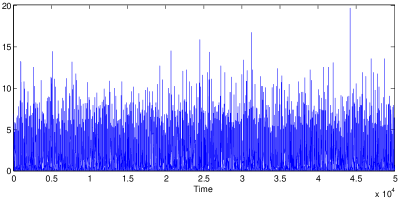
Figure 3: Evolution of $v_{t,T}$ yield by the SO detection method [27] under attack (15) (left) and attack (17) (right).

IX Conclusion

We studied the attack detection problem on stochastic cyber-physical systems. We introduced the definition of asymptotic detectable attacks, as the set of attacks that can be detected by some method based on the knowledge of a single realization, and with probability bigger than zero over the space of realizations. We also characterized this set by providing a necessary and sufficient condition for stochastic detectability. Using this condition, we derived a practically realizable attack detection algorithm. We present simulation results showing how our algorithm can detect attacks that cannot be detected by some simpler methods.

References

- [1] Monish Puthran, Sangeet Puthur, and Radhika Dharulkar. Smart traffic signal. Int. Journal of Comp Sc and Info Tech, 6(2):1360–1363, 2015.
- [2] Alvaro Cardenas, Saurabh Amin, and Shankar Sastry. Research challenges for the security of control systems. In HotSec, 2008.
- [3] Thomas Chen. Stuxnet, the real start of cyber warfare? IEEE Network, 24(6):2–3, 2010.
- [4] C. DeMarco, J. Sariashkar, and F. Alvarado. The potential for malicious control in a competitive power systems environment. In Proc. IEEE Int. Conf. Control Applications, pages 462–467, 1996.
- [5] S. Sridhar, A. Hahn, and M. Govindarasu. Cyberšcphysical system security for the electric power grid. P IEEE, 100(1):210–224, 2012.
- [6] Amir-Hamed Mohsenian-Rad and Alberto Leon-Garcia. Distributed internet-based load altering attacks against smart power grids. IEEE Transactions on Smart Grid, 2(4):667–674, 2011.
- [7] Dan Gyorgy and Henrik Sandberg. Stealth attacks and protection schemes for state estimators in power systems. In IEEE Int. Conf. Smart Grid Communications, pages 214–219, 2010.
- [8] F. Pasqualetti, F. Dorfler, and F. Bullo. Cyber-physical attacks in power networks: Models, fundamental limitations and monitor design. In IEEE Conf. Decision and Control, pages 2195–2201, 2011.
- [9] S Amin, X Litrico, S Sastry, and A Bayen. Stealthy deception attacks on water scada systems. In ACM Conf Hybrid Sys, pages 161–170, 2010.
- [10] D Eliades and M Polycarpou. A fault diagnosis and security framework for water systems. IEEE T Contr Syst T, 18(6):1254–1265, 2010.
- [11] James Farwell and Rafal Rohozinski. Stuxnet and the future of cyber war. Survival, 53(1):23–40, 2011.
- [12] G Richards. Hackers vs slackers. Eng Technol, 3(19):40–43, 2008.
- [13] P Conti. The day the samba stopped. Eng Technol, 5(4):46–47, 2010.
- [14] Jill Slay and Michael Miller. Lessons learned from the maroochy water breach. Critical infrastructure protection, pages 73–82, 2007.
- [15] Svetlana Kuvshinkova. Sql slammer worm lessons learned for consideration by the electricity sector. North American Electric Reliability Council, 1(2):5, 2003.
- [16] Peter Huber. Robust statistics. Springer Berlin Heidelberg, 2011.
- [17] Kemin Zhou, John Doyle, and Keith Glover. Robust and optimal control. New Jersey: Prentice hall, 1996.
- [18] Alan Willsky. A survey of design methods for failure detection in dynamic systems. Automatica, 12(6):601–611, 1976.
- [19] Y Liu, P Ning, and M Reiter. False data injection attacks against state estimation in electric power grids. ACM Transactions on Information and System Security, 14(1):13–14, 2011.
- [20] S Amin, A Cardenas, and S Sastry. Safe and secure networked control systems under denial-of-service attacks. HSCC, 5469:31–45, 2009.
- [21] Y. Mo, E. Garone, A. Casavola, and B Sinopoli. False data injection attacks against state estimation in wireless sensor networks. In 49th IEEE Conference on Decision and Control, pages 5967–5972, 2010.
- [22] A. Teixeira, S. Amin, H. Sandberg, K. Johansson, and S. Sastry. Cyber security analysis of state estimators in electric power systems. In 49th IEEE Conference on Decision and Control, pages 5991–5998, 2010.
- [23] Y Mo and B Sinopoli. Secure control against replay attacks. In Allerton Conf Comm Contr Comp, pages 911–918, 2009.
- [24] Roy Smith. A decoupled feedback structure for covertly appropriating networked control systems. IFAC Proceedings, 44(1):90–95, 2011.
- [25] F Pasqualetti, F Dorfler, and F Bullo. Attack detection and identification in cyber-physical systems. IEEE T Automat Contr, 58(11):2715–2729, 2013.
- [26] F Pasqualetti, F Dorfler, and F Bullo. Attack detection and identification in cyber-physical systems–part ii. arXiv:1202.6049, 2012.
- [27] Y Mo and B Sinopoli. On the performance degradation of cyber-physical systems under stealthy integrity attacks. IEEE T Automat Contr, 61(9):2618–2624, 2016.
- [28] Yilin Mo and Bruno Sinopoli. Secure estimation in the presence of integrity attacks. IEEE T Automat Contr, 60(4):1145–1151, 2015.
- [29] C-Z Bai, V Gupta, and F Pasqualetti. On kalman filtering with compromised sensors: Attack stealthiness and performance bounds. IEEE T Automat Contr, 62(12):6641–6648, 2017.
- [30] Robert M. Gray. Probability, Random Processes, and Ergodic Properties. Springer, 2009.
- [31] Patrick Billingsley. Convergence of Probability Measures. Wiley-Interscience, 1999.
- [32] Achim Klenke. Probability Theory: A Comprehensive Course. Springer, 2013.
- [33] Henry C Thode. Testing for normality, volume 164. CRC press, 2002.
- [34] L Wasserman. All of Statistics: A Concise Course in Statistical Inference. Springer Science, 2004.
- [35] N Bakirov, M Rizzo, and G Székely. A multivariate nonparametric test of independence. J multivariate anal, 97(8):1742–1756, 2006.
- [36] Patrick Billingsley. Probability and measure. John Wiley & Sons, 2008.
- [37] Allen Gersho and Robert M. Gray. Vector Quantization and Signal Compression. Springer, 1991.