Latency Minimization with Optimum Workload Distribution and Power Control for Fog Computing

Abstract

This paper investigates a three-layer IoT-fog-cloud computing system to determine the optimum workload and power allocation at each layer. The objective is to minimize maximum per-layer latency (including both data processing and transmission delays) with individual power constraints. The resulting optimum resource allocation problem is a mixed-integer optimization problem with exponential complexity. Hence, the problem is first relaxed under appropriate modeling assumptions, and then an efficient iterative method is proposed to solve the relaxed but still non-convex problem. The proposed algorithm is based on an alternating optimization approach, which yields close-to-optimum results with significantly reduced complexity. Numerical results are provided to illustrate the performance of the proposed algorithm compared to the exhaustive search method. The latency gain of three-layer distributed IoT-fog-cloud computing is quantified with respect to fog-only and cloud-only computing systems.

I Introduction

The fifth generation ($5$G) of wireless networks and beyond are expected to support billions of connected devices, known as Internet-of-Things (IoT), by using brand-new technologies such as millimeter waves, small cells, multiple antennas, full-duplex and cooperative communications [1, 2, 3, 4]. To achieve this goal, one key challenge is the efficient processing of data generated at the network edge to meet stringent delay and reliability requirements demanded by the wide range of applications. The cloud computing alone is often not enough to meet all the key performance indicators in these emerging use-cases [5, 6, 7]. The fog computing presents a potential solution for this problem by processing data locally at the fog devices.

A typical fog computing architecture can be modeled with three layers of devices: IoT layer, fog layer, and cloud layer [6]. To investigate different aspects of this set-up, various analytic models for control reliability [7], computing delay[8], transmission delay[8], and energy consumption [7, 9, 8] are proposed in the existing literature and references therein. For device-to-device fogging[10], an online task offloading problem is considered to minimize the average energy consumption. In [11], an online joint radio and computational resource management algorithm is developed for multi-user mobile-edge computing systems. In [12], the resource allocation is performed between the end users and their associated small-cell base-stations when they provide cloud-like computing.

For a mobile-edge computing system, the user and data-set size selection is considered to minimize total energy consumption subject to computing latency in [13]. A similar system consisting of single user connected to a computationally capable helper is considered in [14]. In [15], a computing system where the end-users and the cloud are connected via a BS is considered to minimize the energy consumption. A delay-aware and energy efficient computation offloading scheme is proposed in [16] to minimize the consumption of the non-renewable grid energy. In [17], a collaborative computation offloading is studied for cloud and mobile-edge computing to minimize the total energy consumption. The authors in [18] considered a cloud-fog architecture to minimize the maximum computational latency. A trade-off between power consumption and transmission delay in a fog-cloud computing environment is investigated in [8]. Workload allocation strategies within the fog layer subject to a power efficiency constraint are explored in [19].

We note that the fog computing is essentially to complement the cloud computing but not to replace the cloud. In general, even the IoT layer can be equipped with certain computational capabilities. Thus, unlike in existing literature, in this paper, we consider a three-layer IoT-fog-cloud distributed computing architecture, where each layer has its own computational capacity. We investigate the problem of splitting the workload generated by the IoT layer among the IoT, fog, and cloud. The splitting is performed so that the maximum latency at each layer is minimized subject to individual per-layer power constraints. The resulting optimization problem is a mixed-integer program, which is intractable in general. The problem is relaxed with reasonable assumptions. An alternating optimization method is proposed with guaranteed convergence for computing a good feasible point of the relaxed non-convex problem. For all considered empirical scenarios, negligible loss of optimality is recorded. The latency gain due to the IoT-fog-cloud computing is quantified with respect to fog-only and cloud-only systems by using the proposed method.

II System Model

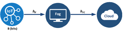
Figure 1: Configuration for three-layer IoT-fog-cloud computing system.

We consider a network consisting of an IoT device (I), a fog node (F), and a cloud server (C), as shown in Fig. 1. While the IoT device has computing resources, it may also offload some of its processing to the fog and cloud layers. We assume that the IoT device has total $B$ [bits] to be processed. It may decide to offload $m$ [bits], $m\leq B$, to the fog node and the fog node in turn may decide to offload $k$ [bits], $k\leq m$, to the cloud node. The workload distribution over the IoT, fog, and cloud layers is then $B-m$, $m-k$ and $k$ [bits], respectively.

Processing time calculations in the proposed fog computing set-up is modelled by introducing computing powers as decision variables. To this end, we start by considering a computing device with processing frequency $f$ [cycles/sec]. Assuming $E_{c}$ [joules/cycle] is required to run each computing cycle, the power consumption for processing data becomes $P_{\rm p}=E_{c}f$ [Watts]. Here $E_{c}$ is considered as an intrinsic device constant depending on the underlying silicon chip technology. Note that $P_{\rm p}$ is the total energy the computing device consumes per second. Extending this naive approach, a more refined model relating $P_{\rm p}$ and $f$ is $P_{\rm p}=af^{\beta}+b$  [Watts], where $\beta$ ranges from $2.5$ to $3$, and $a$ and $b$ are positive constants obtained by curve fitting against empirical measurements [20, 8]. The constant $a$ embodies the effect of $E_{c}$ and other device parameters. Equivalently, $f=\left((P_{\rm p}-b)/a\right)^{\frac{1}{\beta}}$, which is the maximum data processing speed at a given computing power budget $P_{\rm p}$. Now consider executing an algorithm $\mathcal{A}$ with some given complexity $\mathcal{C}(n)$, as a function of the number of input bits $n$ and in units of processor cycles required for algorithm completion. For simplicity, assume that the complexity is linear and given by $\mathcal{C}(n)=cn$ for some positive $c$ [cycles/bit]. Thus, allocating $P_{\rm p}$ to execute $\mathcal{A}$ with $n$ bits requires a time

$$t_{\rm p}=c\ \frac{n}{f}=c\,n\left(\frac{P_{\rm p}-b}{a}\right)^{-\frac{1}{\beta}}\,\,\,\text{[sec]}.$$ (1)

An implicit constraint here is $P_{\rm p}>b$. Let $P_{\rm tI}$, $P_{\rm tF}$ and $P_{\rm tC}$ denote the total power budgets for the IoT, fog, and cloud layers, respectively. Typically, $P_{\rm tI}\ll P_{\rm tF}\ll P_{\rm tC}$. The IoT node needs to allocate $P_{\rm tI}$ for its own data processing and communication with the fog layer. Let the local IoT power allocation for data processing and communication be denoted as $P_{\rm pI}$ and $P_{\rm cI}$, respectively, where $P_{\rm pI}+P_{\rm cI}\leq P_{\rm tI}$. Similarly, power levels $P_{\rm pF}$ and $P_{\rm cF}$ are allocated for data processing and communication at the fog node, respectively, where $P_{\rm pF}+P_{\rm cF}\leq P_{\rm tF}$. Since the cloud only performs data processing at power $P_{\rm pC}$, we require $P_{\rm pC}\leq P_{\rm tC}$. Indexing the $a,b$ and $c$ parameters in (1) with I, F and C, the data processing time at each layer is

$$\text{At I}: ~{}t_{pI}=c_{I}(B-m)\left(\frac{P_{\rm pI}-b_{I}}{a_{I}}\right)^{-\frac{1}{\beta}}\,\,\mbox{ [sec]},$$

$$\text{At F}: ~{}t_{pF}=c_{F}\,(m-k)\left(\frac{P_{\rm pF}-b_{F}}{a_{F}}\right)^{-\frac{1}{\beta}}\,\,\mbox{ [sec]},$$

$$\text{At C}: ~{}t_{pC}=c_{C}\,k\left(\frac{P_{\rm pC}-b_{C}}{a_{C}}\right)^{-\frac{1}{\beta}}\,\,\mbox{ [sec]}.$$

The IoT and fog layers is connected via a wireless link with channel gain $h_{\rm IF}$ and bandwidth $W_{\rm IF}$. The fog communicates with the cloud via a wireless link or an optical link having channel gain $h_{\rm FC}$ and bandwidth $W_{\rm FC}$. The throughputs for the IoT-fog and fog-cloud links are given by

$$\begin{split}\text{I to F}:&~{}R_{\rm IF}=W_{\rm IF}\log_{2}\left(1+\frac{g_{\rm IF}\,P_{\rm cI}}{N_{0}W_{\rm IF}}\right)\ \mbox{[bits/sec]},\\ \text{F to C}:&~{}R_{\rm FC}=W_{\rm FC}\log_{2}\left(1+\frac{g_{\rm FC}\,P_{\rm cF}}{N_{0}W_{\rm FC}}\right)\,\mbox{ [bits/sec]},\end{split}$$

where $g_{\rm IF}{=}|h_{\rm IF}|^{2}$, $g_{\rm FC}{=}|h_{\rm FC}|^{2}$, and $N_{0}$ is the noise spectral density. The communication time over each link is given by

$$t_{\rm c,IF}=\frac{m}{R_{\rm IF}}\,\,\mbox{ [sec]}\,\,\,\text{and}\,\,\,t_{\rm c,FC}=\frac{k}{R_{\rm FC}}\,\,\mbox{ [sec]}.$$ (2)

The total latency at each stage is determined as follows. For local data processing at the IoT layer, we only have latency $T_{\rm I}$ for processing $B-m$ bits. The latency $T_{\rm F}$ for processing $m-k$ bits at the fog layer is the sum of communication latency of $m$ bits from the IoT layer to the fog layer and the processing latency of the $m-k$ bits. For the cloud, the latency $T_{\rm C}$ for processing $k$ bits is the sum of processing time at the cloud and communication latencies from the IoT layer to the fog layer and from the fog layer to the cloud layer. Assuming that data transmission and processing can be carried out simultaneously, the latencies are given by

$$\begin{split}&T_{\rm I}\left(m,P_{\rm pI}\right)=t_{\rm pI};\,\,T_{\rm F}\left(m,k,P_{\rm pF},P_{\rm cI}\right)=t_{\rm c,IF}+t_{\rm pF}\\ &T_{\rm C}\left(m,k,P_{\rm pC},P_{\rm cF}\right)=t_{\rm c,IF}+t_{\rm c,FC}+t_{\rm pC}.\end{split}$$ (3)

Based on (3), the effective system latency to complete the whole task is given by

$$T=\max\left(T_{\rm I},T_{\rm F},T_{\rm C}\right),$$ (4)

where $T$ is a function of workload distribution and power allocations at IoT, fog, and cloud layers.

III Optimum Resource allocation

III-A The Latency Minimization Problem

Our goal is to discover the optimum workload distribution and power allocations at IoT, fog, and cloud layers to minimize $T$. This optimization problem can be formulated as

minimize $$T\left(m,k,P_{\rm pI},P_{\rm cI},P_{\rm pF},P_{\rm cF},P_{\rm pC}\right)$$ (5a)

subject to $$0\leq m\leq B,\ 0\leq k\leq m$$ (6a)

$$P_{\rm pI}+P_{\rm cI}\leq P_{\rm tI},\ P_{\rm pF}+P_{\rm cF}\leq P_{\rm tF}$$ (7a)

$$P_{\rm pI}>b_{I},\ P_{\rm pF}>b_{F},\ b_{C}<P_{\rm pC}\leq P_{\rm tC}$$ (8a)

$$k,m\in\mathbb{Z}\ ,$$ (9a)

where $P_{\rm pI},P_{\rm cI},P_{\rm pF},P_{\rm cF},P_{\rm pC},m$, and $k$ are the decision variables. Note that the optimization problem in (5a) is a mixed-integer nonlinear problem and is intractable in general . However, a plausible strategy, especially when the solution for $m$ and $k$ are expected to be large integers, is to relax the integer constraints [21, p. 307]. More specifically, we consider the related problem by replacing the integer constraint $k,m\in\mathbb{Z}$ of $\eqref{eq:primal-1}$ by $k,m\in\mathbb{R}$, whose epigraph problem is

minimize $$\qquad t$$

subject to $$\qquad T_{\rm I}\left(m,P_{\rm pI}\right)\leq t,\ T_{\rm F}\left(m,k,P_{\rm pF},P_{\rm cI}\right)\leq t,$$ (10)

$$\qquad T_{\rm C}\left(m,k,P_{\rm pC},P_{\rm cF}\right)\leq t$$

$$\qquad\mbox{Constraints \eqref{eq:primal-1-2}-\eqref{eq:primal-1-4}}\ ,$$

with decision variables $t$, $P_{\rm pI}$, $P_{\rm cI}$, $P_{\rm pF}$, $P_{\rm cF}$, $P_{\rm pC}$, $m$, and $k$ [compare with (3) and (4)].

minimize $$\quad t$$

subject to $$\quad c_{I}a_{I}^{(1/\beta)}\displaystyle\frac{B-m}{\displaystyle((1-\alpha)P_{\rm tI}-b_{\rm I})^{\frac{1}{\beta}}}\leq t,\ \frac{m}{\displaystyle W_{\rm IF}\log_{2}\left(1+{\alpha gP_{\rm tI}}\right)}+c_{F}a_{F}^{(1/\beta)}\frac{m-k}{\displaystyle((1-\gamma)P_{\rm tF}-b_{\rm F})^{\frac{1}{\beta}}}\leq t$$ (11)

$$\displaystyle\frac{m}{\displaystyle W_{\rm IF}\log_{2}\left(1+{\alpha gP_{\rm tI}}\right)}+\frac{k}{\displaystyle W_{\rm FC}\log_{2}\left(1+\gamma h{P_{\rm tF}}\right)}+\frac{c_{C}a_{C}^{(1/\beta)}\ k}{\left({P_{\rm tC}-b_{\rm C}}\right)^{\frac{1}{\beta}}}\leq t,\,0\leq m\leq B,\ 0\leq k\leq m,\ \alpha\in[0,\alpha_{\textrm{max}}),\ \gamma\in[0,\gamma_{\textrm{max}}).$$

 

Lemma 1 (Total power usage).

At any optimal point, the power constraints of the problem (10) hold with equality, i.e., $P_{\rm pI}+P_{\rm cI}=P_{\rm tI}$, $P_{\rm pF}+P_{\rm cF}=P_{\rm tF}$ and $P_{\rm pC}=P_{\rm tC}$.

Proof:

The proof is omitted due to space limitations. ∎

Using Lemma 1, the optimization problem in (10) can equivalently be reformulated as in (11), which is at the top of the next page, where the decision variables are $t,\alpha,\gamma,m$, and $k$. The parameters $g=g_{\rm IF}/(N_{0}W_{\rm IF})$ and $h=g_{\rm FC}/(N_{0}W_{\rm FC})$ are introduced for clarity. Although the problem (11) does not exhibit any convexity with respect to the decision variables $t,\alpha,\gamma,m$, and $k$, the problem possesses interesting structural properties that facilitate the application of alternating optimization techniques, as we will discuss next.

III-B Solution Approach: Sequential Latency Minimization

Figure 2: Proposed Sequential Optimization Method: Alternating Stage $1$ and Stage $2$

Figure 3: Proposed Sequential Optimization Method: (Total Processing $+$ Communication) Time Evolution.

For clarity, let $\alpha_{\textrm{max}}=1-{b_{\rm I}}/{P_{\rm tI}}$ and $\gamma_{\textrm{max}}=1-{b_{\rm F}}/{P_{\rm tF}}$. The key step in our method to solve (11) is to decompose the latency minimization (11) into two manageable sub-problems that can be solved sequentially in two stages until a convergence criterion is satisfied. The main idea is illustrated in Fig. 2. Let us consider the first iteration. At stage $1$, the IoT layer solves for the optimum number of bits $m^{(1)}$ (out of $B$) that it can assign to the fog layer, so that the overall time to process $B$ bits at the IoT and fog layers is jointly minimized. In particular, the following problem is solved at stage $1$ of iteration $1$:

minimize $$\quad t$$

subject to $$\quad c_{I}a_{I}^{(1/\beta)}\left[\displaystyle\frac{B-m}{\displaystyle\big{(}[1-\alpha]P_{\rm tI}-b_{\rm I}\big{)}^{\frac{1}{\beta}}}\right]\ \leq t$$

$$\left[\frac{m}{\displaystyle W_{\rm IF}\log_{2}\left(1+{\alpha gP_{\rm tI}}\right)}+\frac{c_{F}a_{F}^{(1/\beta)}\ m}{\displaystyle(P_{\rm tF}-b_{\rm F})^{\frac{1}{\beta}}}\right]\ \leq t$$

$$\quad 0\leq m\leq B,\quad 0\leq\alpha\leq\alpha_{\textrm{max}}\ ,$$ (12)

where the decision variables are $t,m,\alpha$ only and the solution is $(t^{(1)},m^{(1)},\alpha^{(1)})$. The optimization problem (12) is simply (11) with $k=0$, $\gamma=0$, and without the $3$rd constraint. The idea is depicted in Figs. 2 and 3. In this example, the IoT layer requires $7$ [secs] to process $B$ bits alone. After solving stage $1$ optimization problem (12), the IoT and fog layers together require only $5$ [secs] to process $B$ bits, which is around $30$% latency improvement. The latency at stage $1$ includes the processing time of $\left(B{-}m^{(1)}\right)$ bits at the IoT or communication and processing times of $m^{(1)}$ bits at the fog.

In stage $2$ of iteration $1$, the fog solves for the optimum number of bits $k^{(1)}$ that can be assigned to the cloud, so that the overall time to process the already assigned $m^{(1)}$ bits at the fog and cloud are jointly minimized, as illustrated in Fig. 2. In other words, the following is solved at stage $2$ of iteration $1$:

minimize $$\qquad s$$

subject to $$\qquad\frac{m^{(1)}}{\displaystyle W_{\rm IF}\log_{2}\left(1+{gP_{\rm t,I}}\alpha^{(1)}\right)}$$

$$\hskip 75.0001pt+\displaystyle\frac{c_{F}a_{F}^{(1/\beta)}\left(m^{(1)}-k\right)}{\displaystyle((1-\gamma)P_{\rm t,F}-b_{\rm F})^{\frac{1}{\beta}}}\ \leq s$$

$$\qquad\frac{m^{(1)}}{\displaystyle W_{\rm IF}\log_{2}\left(1+{gP_{\rm t,I}}\alpha^{(1)}\right)}+\frac{c_{C}a_{C}^{(1/\beta)}\ k}{\displaystyle(P_{\rm t,C}-b_{\rm C})^{\frac{1}{\beta}}}$$

$$\hskip 65.00009pt+\frac{k}{\displaystyle W_{\rm FC}\log_{2}\left(1+{hP_{\rm t,F}}\gamma\right)}\ \leq s$$

$$\qquad 0\leq k\leq m^{(1)},\ 0\leq\gamma\leq\gamma_{\textrm{max}}\ ,$$ (13)

where the decision variables are $s,k,\gamma$ and the solution is $\left(s^{(1)},k^{(1)},\gamma^{(1)}\right)$. The problem (13) is simply the problem (11), while leaving its first constraint out and considering $m=m^{(1)}$ and $\alpha=\alpha^{(1)}$. Fig. 3 illustrates a situation, where the the aggregate time for communication of $m^{(1)}$ bits from the IoT layer to the fog layer and the processing of ($m^{(1)}-k^{(1)})$ bits at the fog layer is $1$ [sec]. So is the aggregate time to communicate and process $k^{(1)}$ bits at the cloud layer. We observe, however, that the total latency is still $5$ [secs] since the latency at the IoT layer does not improve after solving the second stage optimization problem. This is the status at the end of the first iteration.

To further improve the latency bottleneck at the IoT layer, in the next iteration, we revert to the stage $1$ optimization problem again, which results in $3$ [secs] to process $(B-m^{(1)}-m^{(2)})$ bits at the IoT layer after solving (12) with the updated workload distribution. See Fig. 3. The aggregate communication and processing time of $(m^{(1)}+m^{(2)})$ bits at the fog layer is now equal to $3$ [secs], without any change in the cloud latency. Then, the solution method again proceeds to stage $2$ of the second iteration. The process is thus repeated. Fig. 3 shows the evolution of the aggregate time to process the data at different layers for a case in which the two-stage optimization procedure iterates twice.

Next, we will discuss the properties of the two-stage optimization procedure.

III-C Basis for the Two-Stage Optimization Procedure

Implementation of the proposed solution technique requires solving the stage $1$ and $2$ optimization problems sequentially in an iterative manner. In other words, in any iteration, first the stage $1$ optimization is performed followed by the stage $2$ optimization. The stage $1$ optimization in the $i$th iteration is generally expressed as

minimize $$\quad t$$

subject to $$\quad a_{1i}(\alpha)-b_{1i}(\alpha)m\ \leq t,\ d_{1i}(\alpha)+c_{1i}(\alpha)m\ \leq t$$

$$\textstyle\quad 0\leq m\leq B-\sum_{j=0}^{i-1}m^{(j)}$$ (14)

$$\textstyle\quad 0\leq\alpha\leq\alpha_{\textrm{max}}-\sum_{j=0}^{i-1}\alpha^{(j)}\ ,$$

where the decision variables are $t,m,\alpha$ and the solution is $(t^{(i)},m^{(i)},\alpha^{(i)})$.  The problem parameters $a_{1i},b_{1i},c_{1i}$ and $d_{1i}$ for $i=1,2,\ldots$ are defined in (15) on the next page.

$$a_{1i}(\alpha)=\left[\displaystyle\frac{c_{I}a_{I}^{(1/\beta)}\left(B-\sum_{j=0}^{i-1}m^{(j)}\right)}{\displaystyle\left(\left[1-\textstyle\sum_{j=0}^{i-1}\alpha^{(j)}-\alpha\right]P_{\rm t,I}-b_{\rm I}\right)^{\frac{1}{\beta}}}\right];\,c_{1i}(\alpha)=\frac{1}{\displaystyle W_{\rm IF}\log_{2}\left(1+{gP_{\rm t,I}}\left[\textstyle\sum_{j=0}^{i-1}\alpha^{(j)}+\alpha\right]\right)}+\frac{c_{F}a_{F}^{(1/\beta)}}{\displaystyle\left(\left[1-\textstyle\sum_{j=0}^{i-1}\gamma^{(j)}\right]P_{\rm t,F}-b_{\rm F}\right)^{\frac{1}{\beta}}};$$

$$b_{1i}(\alpha)=\frac{a_{1i}(\alpha)}{B-\sum_{j=0}^{i-1}m^{(j)}};\,d_{1i}(\alpha)=\frac{\sum_{j=0}^{i-1}m^{(j)}}{\displaystyle W_{\rm IF}\log_{2}\left(1+{gP_{\rm t,I}}\left[\textstyle\sum_{j=0}^{i-1}\alpha^{(j)}+\alpha\right]\right)}+\frac{c_{F}a_{F}^{(1/\beta)}\ \sum_{j=0}^{i-1}\left(m^{(j)}-k^{(j)}\right)}{\displaystyle\left(\left[1-\textstyle\sum_{j=0}^{i-1}\gamma^{(j)}\right]P_{\rm t,F}-b_{\rm F}\right)^{\frac{1}{\beta}}}.$$ (15)

 

For a fixed $\alpha$, the solution of (14) can easily be computed by considering the intersection of the lines $a_{1i}(\alpha)-b_{1i}(\alpha)m$ and $d_{1i}(\alpha)+c_{1i}(\alpha)m$. Specifically, $m^{(i)}(\alpha)=\frac{a_{1i}(\alpha)-d_{1i}(\alpha)}{b_{1i}(\alpha)+c_{1i}(\alpha)}$ and $t^{(i)}(\alpha)=\frac{c_{1i}(\alpha)a_{1i}(\alpha)+d_{1i}(\alpha)b_{1i}(\alpha)}{b_{1i}(\alpha)+c_{1i}(\alpha)}$. Based on these, $\alpha^{(i)}$ which solves (14) is given by

$$\alpha^{(i)}=\displaystyle\mathop{\textstyle{\mbox{argmin}}}_{0\leq\alpha\leq\alpha_{\textrm{max}}-\sum_{j=0}^{i-1}\alpha^{(j)}}\ \ t^{(i)}(\alpha),$$ (16)

which can be computed by using a scalar grid search over the range of $\alpha$. Substituting $\alpha^{(i)}$ yields the solutions $m^{(i)}$ and $t^{(i)}$ for (14), respectively.

Similarly, the stage $2$ optimization in the $i$th iteration is

minimize $$\quad s$$

subject to $$\quad L_{2i}+a_{2i}(\gamma)-b_{2i}(\gamma)k\ \leq s$$

$$\quad L_{2i}+d_{2i}(\gamma)+c_{2i}(\gamma)k\ \leq s$$

$$\textstyle\quad 0\leq k\leq\sum_{j=0}^{i}m^{(j)}-\sum_{j=0}^{i-1}k^{(j)}$$ (17)

$$\textstyle\quad 0\leq\gamma\leq\gamma_{\textrm{max}}-\sum_{j=0}^{i-1}\gamma^{(j)}\ ,$$

where the decision variables are $s,k,\gamma$ and the solution is $(s^{(i)},k^{(i)},\gamma^{(i)})$. The problem parameters $a_{2i},b_{2i},c_{2i}$, $d_{2i}$ and $L_{2i}$ for $i=1,2,\ldots$ are given in (18) shown on the next page.

$$a_{2i}(\gamma)=c_{F}a_{F}^{(1/\beta)}\left[\displaystyle\frac{\left(\sum_{j=0}^{i}m^{(j)}{-}\sum_{j=0}^{i-1}k^{(j)}\right)}{\displaystyle\left(\left[1{-}\textstyle\sum_{j=0}^{i-1}\gamma^{(j)}{-}\gamma\right]P_{\rm t,F}-b_{\rm F}\right)^{\frac{1}{\beta}}}\right];\,c_{2i}(\gamma)=\frac{1}{\displaystyle W_{\rm FC}\log_{2}\left(1+{hP_{\rm t,F}}\left[\textstyle\sum_{j=0}^{i-1}\gamma^{(j)}+\gamma\right]\right)}+\frac{c_{C}a_{C}^{(1/\beta)}}{\displaystyle\left(P_{\rm t,C}-b_{\rm C}\right)^{\frac{1}{\beta}}},;$$

$$b_{2i}(\gamma)=\frac{a_{2i}(\gamma)}{\sum_{j=0}^{i}m^{(j)}{-}\sum_{j=0}^{i-1}k^{(j)}};\,d_{2i}(\gamma)=c_{2i}(\gamma)\sum_{j=0}^{i-1}k^{(j)};\,L_{2i}=\frac{\sum_{j=0}^{i}m^{(j)}}{\displaystyle W_{\rm IF}\log_{2}\left(1+{gP_{\rm t,I}}\left[\textstyle\sum_{j=0}^{i}\alpha^{(j)}\right]\right)}.$$ (18)

 

Steps for computing the solution $(s^{(i)},k^{(i)},\gamma^{(i)})$ for (17) are similar to those for computing $(t^{(i)},m^{(i)},\alpha^{(i)})$ in (14). In particular, $k^{(i)}(\gamma)=\frac{a_{2i}(\gamma)-d_{2i}(\gamma)}{b_{2i}(\gamma)+c_{2i}(\gamma)}$ and $s^{(i)}(\gamma)=\frac{c_{2i}(\gamma)a_{2i}(\gamma)+d_{2i}(\gamma)b_{2i}(\gamma)}{b_{2i}(\gamma)+c_{2i}(\gamma)}+L_{2i}$, which are used to determine $(s^{(i)},k^{(i)},\gamma^{(i)})$. The optimal point $\gamma^{(i)}$ of (17) is given by

$$\gamma^{(i)}=\displaystyle\mathop{\textstyle{\mbox{argmin}}}_{0\leq\gamma\leq\gamma_{\textrm{max}}-\sum_{j=0}^{i-1}\gamma^{(j)}}\ \ s^{(i)}(\gamma),$$ (19)

and $k^{(i)}$, $s^{(i)}$ are computed by evaluating their expressions at $\gamma^{(i)}$.

III-D Sequential Latency Minimization (SLM) Algorithm

In this section, based on the results in § III-C, we outline the sequential latency minimization (SLM) algorithm followed by its convergence properties.

Algorithm 1 SLM Algorithm

1:Initialization: Set $i=1$, $(m^{(i-1)},\alpha^{(i-1)})=(0,0)$ and $(k^{(i-1)},\gamma^{(i-1)})=(0,0)$. Let $\epsilon>0$ be an accuracy level.

2:Solve problem (14) to yield $t^{(i)},m^{(i)}$ and $\alpha^{(i)}$.

3:Solve problem (17) to yield $s^{(i)},k^{(i)}$ and $\gamma^{(i)}$.

4:If $|t^{(i)}-s^{(i)}|\leq\epsilon$, go to step $5$. Otherwise, set $i=i+1$ and go to step 2.

5:Output: Let $t^{\star}{=}t^{(i)}$, $m^{\star}=\sum_{j=0}^{i}m^{(j)}$, $k^{\star}=\sum_{j=0}^{i}k^{(j)}$, $\alpha^{\star}=\sum_{j=0}^{i}\alpha^{(j)}$, and $\gamma^{\star}=\sum_{j=0}^{i}\gamma^{(j)}$ and STOP.

The SLM algorithm is summarized in Algorithm 1. Step $1$ initializes the SLM. Steps $2$ and $3$ are the stage $1$ and stage $2$ optimization problems, respectively. The stopping criterion is checked at step $4$. Finally, step $5$ computes the aggregate workload at the fog and cloud layers $m^{\star}$ and $k^{\star}$, together with the power split values at the IoT and fog layers $\alpha^{\star}$ and $\gamma^{\star}$, respectively. The associated latency is given by $t^{\star}$. The SLM algorithm always terminates after finitely many iterations, as shown in Theorem 1, which is a consequence of following lemmas.

Lemma 2.

For any positive integer $i$, $t^{(i)}\geq s^{(i)}$.

Proof:

This follows simply by noting that $s=t^{(i)}$, $k=0$, and $\gamma=0$ is feasible for problem (17). Thus, the optimal value $s^{(i)}$ of problem (17) no greater than $t^{(i)}$. ∎

Lemma 3.

The sequence ${t^{(i)}}$ is strictly monotonically decreasing and bounded below. Moreover, the sequence ${s^{(i)}}$ is strictly monotonically increasing and bounded above.

Proof:

Only an outline of the proof is provided. At the end of the first iteration, $t^{(1)}\geq s^{(1)}$ according to Lemma 2. If $t^{(1)}=s^{(1)}$, the algorithm exits. Otherwise, $t^{(1)}>s^{(1)}$. Assuming this is the case, consider the second iteration. To solve the stage $1$ problem, the left-hand sides of the first two inequalities in (14) must be set equal, which leads to $t^{(1)}>t^{(2)}>s^{(1)}$. Similarly, to solve the stage $2$ problem in (17), the left-hand sides of the first two inequality constraints must be balanced, and thus $s^{(1)}<s^{(2)}<t^{(2)}$. Therefore, at the end of the second iteration, $t^{(2)}<t^{(1)},s^{(2)}>s^{(1)}$. The iterations continue in this manner and the proof is concluded. ∎

Theorem 1.

The SLM algorithm terminates in finite time. In particular, $\lim_{i\rightarrow\infty}\left(t^{(i)}-s^{(i)}\right)=0.$

Proof:

The proof is based on Lemma 3. ∎

IV Numerical results

In this section, numerical examples are provided to compare SLM algorithm and the optimum exhaustive search method. We consider a computing scenario in which the IoT, fog, and cloud layers are implemented with processors Quark X1000 400 MHz, Xeon E7450 Dunnington $2.4$ GHz, and Xeon Platinum 8156-Intel $3.6$ GHz, respectively, with maximum power dissipations of $2.2$ W, $90$ W, and $105$ W, as given in various Intel CPU specifications. According to (1), we select $a_{I}$, $a_{F}$ and $a_{C}$ to satisfy these maximum powers for $\beta=3$ and $b_{I}=b_{F}=b_{C}=10^{-3}$. The signal-to-noise ratios (SNRs) of the links between the IoT and fog layers and the fog and cloud layers are defined as $\text{SNR}_{\rm IF}={P_{\rm tI}}/{(N_{0}W_{\rm IF})}$ and $\text{SNR}_{\rm FC}={P_{\rm tF}}/{(N_{0}W_{\rm FC})}$, respectively. The wireless channel gain between the IoT and fog layers is exponentially distributed with unit mean. We set other parameters as $c_{I}=5$, $c_{F}=2$, $c_{C}=1$, $W_{\rm IF}=W_{\rm FC}=500$ MHz, $\text{SNR}_{\rm FC}=32$ dB, and $N_{0}=10^{-10}$ Watts/Hz. We calculate the average latency over 4000 channel realizations.

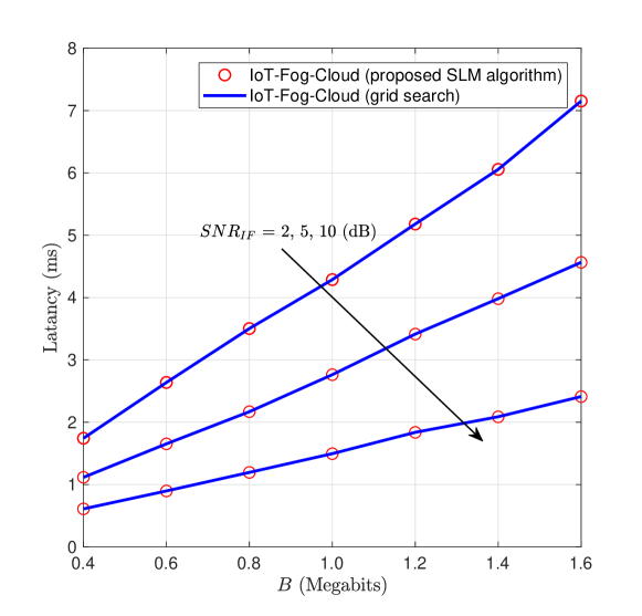
Figure 4: The average latency vs workload $B$ for different $\text{SNR}_{\rm IF}$.

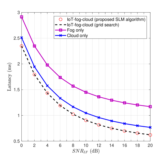
Figure 5: The average latency vs $\text{SNR}_{\rm IF}$ for different computing systems.

Figure 4 shows the average latency (in milli-seconds) vs workload $B$ (in Megabits) for both the proposed SLM algorithm and the optimal grid search when $\text{SNR}_{\rm IF}=2,5,10$ dB. The optimum value is obtained through the exhaustive two-dimensional grid search with a granularity of $10^{-2}$ in each dimension. Clearly, the results of both methods coincide, which suggests that the SLM algorithm performs very close to the optimum method. Figure 4 also indicates that the latency increases almost linearly with workload $B$. For example, for the simulated range at $\text{SNR}_{\rm IF}=5$ dB, latency increases from $1.1$ ms to $4.5$ ms, where we need $2.9$ ms to process one Megabits of data. Further, to achieve 2 ms latency, we can process approximately 0.45, 0.75 and 1.35 Megabits when $\text{SNR}_{\rm IF}=2,5,10$ dB, respectively.

Figure 5 depicts the average latency (in milli-seconds) vs $\text{SNR}_{\rm IF}$ when workload $B=1$ Megabits. It compares three different architectural choices: i) IoT-fog-cloud; ii) fog-only; and iii) cloud-only. The average latency decreases when $\text{SNR}_{\rm IF}$ increases, as expected. Results shows that the IoT-fog-cloud computing architecture always outperforms others. For example, to yield a $1$ ms latency, the IoT-fog-cloud computing system requires $\text{SNR}_{\rm IF}=8$ dB, whereas the cloud-only computing system needs $\text{SNR}_{\rm IF}=11$ dB. The fog-only computing system cannot yield a $1$ ms latency even when $\text{SNR}_{\rm IF}=20$ dB. The IoT-fog-cloud computing architecture always yields a decrease in the latencies, irrespective of $\text{SNR}_{\rm IF}$. For example, at $\text{SNR}_{\rm IF}=16$ dB, the increase in latencies of the fog-only and cloud-only computing systems, compared to the IoT-fog-cloud computing system is $79$% and $21$%, respectively.

V Conclusion

The power and workload allocation problem to minimize data processing latency for a three-layer IoT-fog-cloud computing systems was investigated. The resulting problem is non-convex. To devise an efficient solution method, a constraint relaxation was considered yielding, under reasonable grounds, a very good approximation to the original problem formulation. A sequential latency minimization (SLM) algorithm based on alternating optimization was proposed to handle the relaxed problem. Convergence of the SLM algorithm was established. Numerical results suggested that the performance of SLM algorithm was almost identical to that of the optimum exhaustive search method for the relaxed problem. Finally, we evaluated numerically the gains of the three-layer IoT-fog-cloud computing over fog-only and cloud-only computing, in terms of data processing latencies. Results suggest that the three-layer computing is more potent, for yielding better latencies, than fog-only or cloud-only computing systems.

References

- [1] L. Liu, R. Chen, S. Geirhofer, K. Sayana, Z. Shi, and Y. Zhou, “Downlink MIMO in LTE-advanced: SU-MIMO vs. MU-MIMO,” IEEE Commun. Mag., vol. 50, no. 2, pp. 140–147, Feb. 2012.
- [2] S. Rangan, T. S. Rappaport, and E. Erkip, “Millimeter-wave cellular wireless networks: Potentials and challenges,” Proc. the IEEE, vol. 102, no. 3, pp. 366–385, Mar. 2014.
- [3] S. Atapattu, Y. Jing, H. Jiang, and C. Tellambura, “Relay selection and performance analysis in multiple-user networks,” IEEE J. Select. Areas Commun., vol. 31, no. 8, pp. 1517–1529, Aug. 2013.
- [4] S. Atapattu, P. Dharmawansa, M. Di Renzo, C. Tellambura, and J. S. Evans, “Multi-user relay selection for full-duplex radio,” IEEE Trans. Commun., vol. 67, no. 2, pp. 955–972, Feb. 2019.
- [5] M. Chiang and T. Zhang, “Fog and IoT: An overview of research opportunities,” IEEE Internet Things J., vol. 3, no. 6, pp. 854–864, Dec. 2016.
- [6] M. Gorlatova, H. Inaltekin, and M. Chiang, “Characterizing task completion latencies in fog computing,” Technical Report, Nov. 2018. [Online]. Available: https://arxiv.org/abs/1811.02638.
- [7] H. Inaltekin, M. Gorlatova, and M. Chiang, “Virtualized control over fog: Interplay between reliability and latency,” IEEE Internet of Things J., vol. 5, no. 6, pp. 5030–5045, Dec. 2018.
- [8] R. Deng, R. Lu, C. Lai, T. H. Luan, and H. Liang, “Optimal workload allocation in fog-cloud computing toward balanced delay and power consumption,” IEEE Internet of Things J., vol. 3, no. 6, pp. 1171–1181, Dec. 2016.
- [9] F. Jalali, K. Hinton, R. Ayre, T. Alpcan, and R. S. Tucker, “Fog computing may help to save energy in cloud computing,” IEEE J. Select. Areas Commun., vol. 34, no. 5, pp. 1728–1739, May 2016.
- [10] L. Pu, X. Chen, J. Xu, and X. Fu, “D2D fogging: An energy-efficient and incentive-aware task offloading framework via network-assisted D2D collaboration,” IEEE J. Select. Areas Commun., vol. 34, no. 12, pp. 3887–3901, Dec. 2016.
- [11] Y. Mao, J. Zhang, S. H. Song, and K. B. Letaief, “Stochastic joint radio and computational resource management for multi-user mobile-edge computing systems,” IEEE Trans. Wireless Commun., vol. 16, no. 9, pp. 5994–6009, Sep. 2017.
- [12] L. Chen, S. Zhou, and J. Xu, “Computation peer offloading for energy-constrained mobile edge computing in small-cell networks,” IEEE/ACM Trans. Networking, vol. 26, no. 4, pp. 1619–1632, Aug. 2018.
- [13] C. You, K. Huang, H. Chae, and B. Kim, “Energy-efficient resource allocation for mobile-edge computation offloading,” IEEE Trans. Wireless Commun., vol. 16, no. 3, pp. 1397–1411, Mar. 2017.
- [14] Y. Tao, C. You, P. Zhang, and K. Huang, “Stochastic control of computation offloading to a dynamic helper,” in Proc. IEEE Int. Conf. Commun. Workshops (ICC Workshops), May 2018.
- [15] N. T. Ti and L. B. Le, “Computation offloading leveraging computing resources from edge cloud and mobile peers,” in Proc. IEEE Int. Conf. Commun. (ICC), May 2017.
- [16] X. He, Y. Chen, and K. K. Chai, “Delay-aware energy efficient computation offloading for energy harvesting enabled fog radio access networks,” in Proc. IEEE Vehicular Technology Conf. (VTC), Jun. 2018.
- [17] H. Guo and J. Liu, “Collaborative computation offloading for multiaccess edge computing over fiber–wireless networks,” IEEE Trans. Veh. Technol., vol. 67, no. 5, pp. 4514–4526, May 2018.
- [18] G. Lee, W. Saad, and M. Bennis, “An online secretary framework for fog network formation with minimal latency,” in Proc. IEEE Int. Conf. Commun. (ICC), May 2017.
- [19] Y. Xiao and M. Krunz, “QoE and power efficiency tradeoff for fog computing networks with fog node cooperation,” in Proc. IEEE INFOCOM, May 2017.
- [20] L. Rao, X. Liu, M. D. Ilic, and J. Liu, “Distributed coordination of internet data centers under multiregional electricity markets,” IEEE Proc., vol. 100, no. 1, pp. 269–282, Jan. 2012.
- [21] C. H. Papadimitriou and K. Steiglitz, Combinatorial Optimization: Algorithms and Complexity. Englewood Cliffs New Jersey: Prentice-Hall, 1982.