Visualizing Free Energy Landscapes for Four Hard Disks

Abstract

We present a simple model system with four hard disks moving in a circular region for which free energy landscapes can be directly calculated and visualized in two and three dimensions. We construct several energy landscapes for our system and explore the strengths and limitations of each in terms of understanding system dynamics, in particular the relationship between state transitions and free energy barriers. We also demonstrate the importance of distinguishing between system dynamics in real space and those in landscape coordinates, and show that care must be taken to appropriately combine dynamics with barrier properties to understand the transition rates. This simple model provides an intuitive way to understand free energy landscapes, and illustrates the benefits free energy landscapes can have over potential energy landscapes.

I Introduction

Energy landscapes are of widespread utility for science, relevant for understanding condensed matter systems goldstein69 ; sciortino05 ; desouza08 , protein folding bryngelson95 ; berry97 ; joseph17 , chemical reactions marcelin1914 ; awasthi19 , optimization problems krzakala07 , and even machine learning ballard17 . The first proposal related to energy landscapes dates back to René Marcelin, a French physical chemist who in 1914 proposed understanding chemical kinetics in terms of the Lagrangian coordinates describing atomic motions marcelin1914 ; laidler85 . Marcelin’s idea was “mouvement des points représentatifs dans l’espace à $2N$ dimensions” – “movement of representative points in $2N$-dimensional space,” where $N$ is the number of Lagrangian generalized coordinate pairs. More modern descriptions of energy landscapes date from 1969, when Martin Goldstein re-introduced the concept goldstein69 . Goldstein considered a situation with $N$ particles in a three-dimensional space, with some potential energy $U$ of interaction between the particles. To quote, “When I speak of the potential energy surface I refer to $U$ plotted as a function of $3N$ atomic coordinates in a $3N+1$ dimensional space.” That is, $U$ is a function of the $x,y,$ and $z$ positions of all $N$ particles (a total of $3N$ numbers), so graphing $U$ forms a surface in this very high dimensional space.

Picturing this high dimensional surface is of course challenging. The first picture the authors are aware of was published by Stillinger and Weber in 1984 stillinger84 , and is shown in Fig. 1. Here the surface is represented as the height as a function of two coordinates, giving rise to the terminology of calling this the “energy landscape.” The solid lines are contours of constant $U$. The dashed lines enclose local minima of the surface; the nodes where the dashed lines connect are local maxima. $\times$’s mark saddle points between local minima. For a thermal system, particles can transition from one configuration to another by a thermal fluctuation that carries them over a dashed line, perhaps crossing near a saddle point. The transition in the $3N$-dimensional space encodes the appropriate changes of the coordinates in real space of the $N$ particles. Stillinger and Weber were interested in studying liquids, so accordingly the disordered appearance of Fig. 1 represents the complex dependence of $U$ on the amorphous liquid structure.

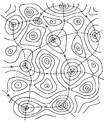
Figure 1: Sketch of a potential energy surface as a function of two coordinates. The solid lines are contours of constant $U$. The dashed lines separate local minimal (solid circles) and connect at local maxima. Saddle points are marked with $\times$. From Stillinger and Weber, Science 225, 983-989 (1984) stillinger84 . Reprinted with permission from AAAS.

A few years later, the challenge of drawing a surface as a function of $3N$ coordinates was further simplified to a curve in 1 dimension; a 1988 example from Stillinger is shown in Fig. 2 stillinger88 . Here the lowest energy state corresponds to a crystal – the ground state. In contrast, there are many disordered glassy states and they have higher potential energy. The states at the right represent regions of phase space that correspond to particular configurations of the $N$ atoms with slightly lower $U$, but nonetheless which are amorphous and thus far from the crystal configuration which minimizes $U$. Later work generalized this type of sketch to be more random in appearance (for example, Ref. stillinger95 ), with the general understanding that this one-dimensional landscape sketch is supposed to convey a complex high-dimensional surface.

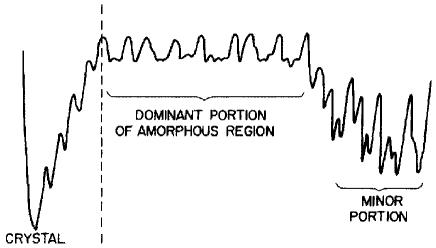
Figure 2: Sketch of a potential energy surface as a function of one coordinate. This particular sketch represents different possible characters of the phase space, including a crystalline state (left) and amorphous states (middle and right). Reprinted from F. H. Stillinger, J. Chem. Phys. 88, 7818 (1988) stillinger88 , with the permission of AIP Publishing.

A conceptual simplification comes from considering the $N$ objects not to be atoms but rather hard spheres. Hard spheres have no attractive interaction, and repel each other if they touch. The potential energy $U$ for hard spheres is zero if they do not overlap, and infinite if they do overlap. This system can be ordered into a crystal or disordered like a liquid or glass, and so has interesting phase behavior alder57 ; wood57 ; bernal64 ; widom67 ; pusey86 . In this situation, there are still $3N$ coordinates. As a function of these coordinates, $U$ is either zero or infinite, with $U=\infty$ representing forbidden configurations where two or more particles overlap. Now transitions between states no longer require crossing saddle points where $U$ is slightly higher; rather, transitions between states require passing through entropic bottlenecks zhou91 ; hunter12pre . One can think of a free energy, $F=U-TS$, where $T$ is the absolute temperature and $S$ is the entropy. States with high $S$ (thus low $F$) correspond to common configurations of the hard spheres, and states with low $S$ correspond to rare configurations. One would have to understand what would be meant by a common or rare configuration of the $3N$ coordinates, and it is not obvious how a sketch of $F$ would differ (if at all) from something like Figs. 1 or 2. While hard spheres are a conceptual simplification, it does not necessarily make understanding the free energy landscape any simpler.

The earliest mention of free energy landscapes that we are aware of was Hill and Eisenberg in 1976, who considered “free energy surfaces” in myosin-actin-ATP systems hill76 . They projected the behavior of the system down to a few important coordinates. For example, at one point they discuss the free energy of a molecule based on one coordinate, “statistically averaged over all possible configurations of all solvent molecules and over the rotational coordinates of the ligand.” Later work was more explicit about the landscape analogy; for example Bryngelson and Wolynes in 1987, also considering a biological system (protein folding), discuss ideas such as moving downhill to a local minimum of the free energy. Other work in the 1980’s and 1990’s talked about free energy landscapes but gloss over the difference between that and a potential energy landscape; these authors mainly consider free energy landscapes as they had methods to calculate the free energy as a function of coordinates soukoulis82 ; paine85 ; fontana91 . A common approach for free energy is to consider just one or two “reaction coordinates” or “order parameters” that describe a behavior of interest, such as protein folding or a chemical reaction wales03 . A recent review explicitly addressing both potential energy and free energy landscapes notes that for the latter, one constructs a free energy landscape by “by averaging over most of the coordinates” wales06 . The main benefit of free energy landscapes is to focus attention on a small number of meaningful coordinates.

Figure 3: (Color online) Illustration of our model system, with four hard disks confined to a two dimensional circular region. The disks have radius equal to 1, and the circular region has a radius $3+\epsilon$; in this sketch $\epsilon=0.3$.

In this paper we present a model system using four hard disks which has nontrivial dynamics and a nontrivial free energy landscape. The potential energy landscape as a function of the $2N=8$ coordinates can be usefully projected down to three or even two dimensions so that a free landscape can be directly visualized, rather than needing a conceptual sketch. We use this model system to illustrate several ideas about free energy landscapes. For example, a key point is that this projection operation is not unique: there are multiple possible ways to visualize the free energy landscape, with varying utility. We verify that similar results are obtained for diffusive dynamics and ballistic dynamics. Our model is in the spirit of other simple models involving very small numbers of particles hunter12pre ; giarritta94 ; speedy94 ; bowles99 ; bowles06 ; ashwin09 ; carlsson12 ; barnettjones13 ; hinow14 ; godfrey14 ; godfrey15 ; robinson16 .

II Dynamics of the model system

Figure 3 shows the model system, comprised of four hard disks confined to a two-dimensional circular region; this is an extension of a previous model with three hard disks hunter12pre . We let the disks move, subject to the constraint that no disk can overlap another disk or overlap the boundary of the system. The disks are distinguishable, so there are six “equilibrium” states, shown in Fig. 4. Changing from one state to another requires one of the disks to move through the middle of the system so as to swap locations with one of its neighbors. Examples of these swaps are shown in Fig. 5(a-e) and Fig. 6(a-e). Swapping locations requires a large enough system for this to occur: three disks must be able to align momentarily as the middle one passes through the other two. We define the disks all to have radius 1, and then the minimum system size is radius $R=3$. A smaller $R$ is possible, but then no rearrangements can occur. A larger system makes rearrangements easier, so accordingly we define the system radius to be $R=3+\epsilon$. Letting $\epsilon\rightarrow 0$ results in behavior a bit like a crystalline or glassy system, in that particles become unable to rearrange, although they can still vibrate locally.

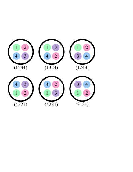
Figure 4: (Color online) The six distinct “equilibrium” states, labeled by the order of the disks in a clockwise direction. The bottom row of states are mirror images of the top row. At any given moment it is unlikely that the four particles are exactly arranged in a square, but rather these states should be understood as the situations where the order of the four particles is well defined. Likewise, rotations of these states are considered equivalent; only the order matters. For example, the state shown in Fig. 3 is (1243).

We use two simulation methods. The first method approximates diffusive motion for the particles, and will be used for most of the results presented in this paper. In this simulation, we consider a small trial move for a disk in a random direction. This move is accepted if the new position does not overlap any other disk or the boundary, and otherwise is rejected. A simulation time step occurs when we have considered one trial move for each of the four disks (picked in random order at each time step). We choose a step size of $L=10^{-2.5}$ so that most steps are accepted, and verify that our results are insensitive to this choice. With this choice, the time it takes for a free particle to diffuse in the $x$ (or $y$) coordinate a distance 1 is given by $\tau_{D}=1/L^{2}=10^{5}$ time steps. Accordingly, we define our time in units of $\tau_{D}$. We run our simulations for $10^{4}-10^{5}\tau_{D}$, long enough for at least 20 rearrangements to occur, and often $100-1000$ rearrangements, depending on $\epsilon$. As will be seen, the smaller $\epsilon$ is the longer it takes for a rearrangement to occur.

The second simulation method computes ballistic trajectories for each disk using an event-driven computation. For this simulation, the four disks are initialized with velocities $v=1$ in random directions, but with the constraint that the total angular momentum is zero. We calculate the next time for each possible collision (disk-disk or disk-wall) and advance the positions of the four particles to the earliest collision. The velocity of the colliding particle(s) are updated conserving energy and momentum. Where these results are presented in this paper, time is in units of $\tau_{v}=1/v=1$, the time it takes a non-colliding particle to move a distance of 1 (the disk radius) based on the initial velocity scale $v$; note that the instantaneous velocity of the disks fluctuate due to the collisions, albeit with the total kinetic energy constant.

There are many possible ways to project from the 8-dimensional phase space in the disk coordinates down to lower dimensions. One needs to map from the four original positions down to a smaller number of coordinates. We choose to use vector operations. Relative positions are describable by vectors pointing from disks $i$ to disks $j$:

$$\vec{v}_{ij}=(x_{j}-x_{i},y_{j}-y_{i}).$$ (1)

With $i\neq j$, this is a set of six vectors (ignoring the counterparts in opposite direction, that is, using $\vec{v}_{12}$ and not $\vec{v}_{21}=-\vec{v}_{12}$). While many operations could be done with these vectors to generate landscape coordinates, it is easiest to consider working with pairs of vectors: there are 15 such pairs. It also is useful to require each pair of vectors to depend on the coordinates of all four particles: this reduces the number of distinct pairs to 3. That is, considering the pair ($\vec{v}_{12},\vec{v}_{13}$) is not desirable as it tell us nothing about particle 4, whereas the pair ($\vec{v}_{12},\vec{v}_{34}$) has some information about all four particles. Finally, we will consider the two straightforward vector operations to act on each pair of vectors: the cross product and the dot product, which will each result in a distinct free energy landscape.

We first consider the cross product, and will use this initially to illustrate the system dynamics. We compute the vector cross products:

$$c_{1} = (\vec{v}_{12}\times\vec{v}_{34})\cdot\hat{z},$$ (2)

$$c_{2} = (\vec{v}_{13}\times\vec{v}_{42})\cdot\hat{z},$$

$$c_{3} = (\vec{v}_{14}\times\vec{v}_{23})\cdot\hat{z},$$

where the final dot product with $\hat{z}$ ensures that the $c$’s are scalars; $\hat{z}$ is the unit vector perpendicular to the two-dimensional system. For the equilibrium configurations shown in Fig. 4, the $c$’s are positive, negative, or roughly zero depending on the arrangement of the four disks. For example, if the disks are arranged in a square of side length $s$, with the disks arranged (1243), then $c_{1}=+2s^{2}$, $c_{2}=c_{3}=0$. If the disks are arranged in the opposite order (3421), then $c_{1}=-2s^{2}$ and $c_{2}=c_{3}=0$. Likewise $c_{2}$ and $c_{3}$ are each nonzero for two opposite pairs of configurations, and zero for the other four.

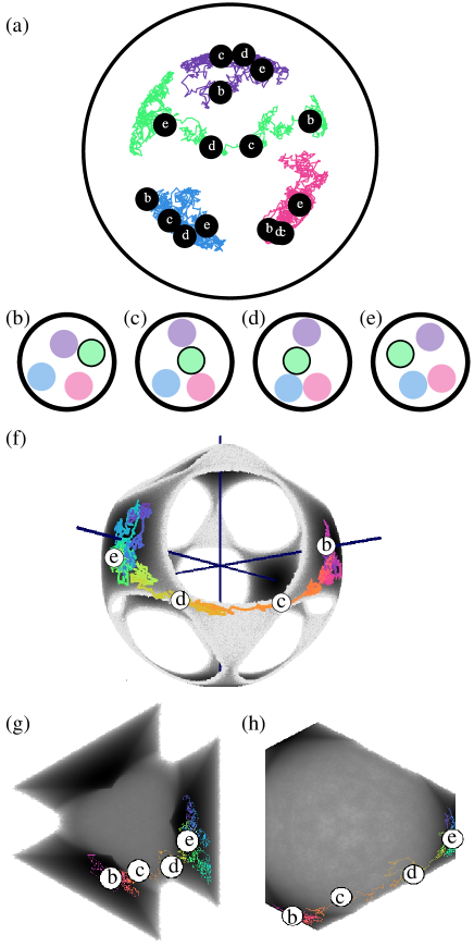
Figure 5: (Color online) (a) Real space trajectories during a transition with system size $\epsilon=0.18$ and using diffusive dynamics. The letters correspond to the snapshots of the system shown in panels (b-e). In this transition $(1243)\rightarrow(1324)$, the outlined disk moves through the middle. The total time pictured is $10\tau_{D}$, and steps are drawn spaced by $\Delta t=0.01\tau_{D}$. (f) Free energy landscape in the variables $(c_{1},c_{2},c_{3})$. (g) Free energy landscape in the variables $(d_{1},d_{2})$. (h) Free energy landscape in the variables $(u_{1},u_{2})$. In panels (f,g,h), the positions corresponding to snapshots (b) through (e) are marked.

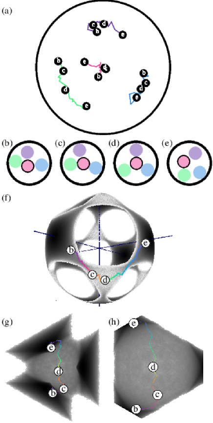
Figure 6: (Color online) (a) Real space trajectories during a transition with system size $\epsilon=0.20$ and using ballistic dynamics. Letters correspond to the snapshots shown in panels (b-e). In this transition $(3421)\rightarrow(1234)$, the outlined disk moves through the middle. The total time pictured is $4\tau_{v}$. (f) Free energy landscape in the variables $(c_{1},c_{2},c_{3})$. (g) Free energy landscape in the variables $(d_{1},d_{2})$. (h) Free energy landscape in the variables $(u_{1},u_{2})$. In panels (f,g,h), the positions corresponding to snapshots (b) through (e) are marked. Note that the phase space trajectory in (f) has been rotated; in particular this is a different perspective than shown in Fig. 5(f).

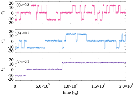
Figure 7: (Color online) Trajectories of the coordinate $c_{1}$ as a function of time, for system sizes $\epsilon$ as indicated, using diffusive dynamics. Transitions indicate one of the disks passing through the middle of the system. Note that $c_{1}$ is zero for four of the six states shown in Fig. 4, so some transitions that keep $c_{1}=0$ are not apparent in the data, but would be apparent in plots of $c_{2}$ and $c_{3}$.

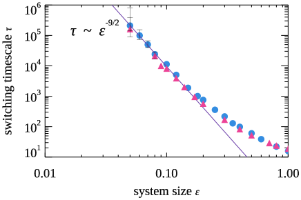
Figure 8: (Color online) The switching timescale $\tau$ as a function of the system size $\epsilon$, for diffusive dynamics (circles, in units of $\tau_{D}$) and ballistic dynamics (triangles, in units of $\tau_{v}$). As $\epsilon\rightarrow 0$ the timescale grows as $\epsilon^{-9/2}$ as indicated by the solid line. The uncertainties are 95% confidence intervals; where not shown, the uncertainties are smaller than the symbol size.

Before constructing a free energy landscape with these coordinates, first consider the behavior of the system viewed through one of these coordinates, shown in Fig. 7. For a relatively large system size [panel (a), $\epsilon=0.3$], transitions happen fairly frequently. As the system size is decreased, panels (b) and (c) show transitions happen less frequently. This is because there is less ability for the disks to find a configuration where one disk passes through the middle of the system to swap places with one of the others.

Figure 8 shows the mean time $\tau$ between switching states as a function of the system size $\epsilon$. As $\epsilon\rightarrow 0$ the switching time grows larger, confirming the qualitative picture of Fig. 7. It is perhaps a bit of a coincidence that as a function of $\epsilon$ the magnitude of $\tau$ is similar for diffusive dynamics (circles, in terms of $\tau_{D}$) and ballistic dynamics (triangles, in terms of $\tau_{v}$). The particular power law dependence $\tau\sim\epsilon^{-9/2}$ will be explained in Sec. IV.

The behavior appears similar to a glass transition, in that the time scale for rearrangement grows dramatically as $\epsilon\rightarrow 0$. As a molten glass is cooled, its viscosity grows dramatically – which is to say, the time scale for internal rearrangements grows dramatically sciortino05 ; ediger12 ; biroli13 . The previous three disk model (which inspired this four disk model) was designed to capture the basic crowding that can lead to a glass transition hunter12pre . The coordinated motion of the four disks during a transition from one basic state to another conceptually resembles what is seen in simulations of materials close to the glass transition desouza08 ; donati98 ; doliwa00 .

III Free Energy Landscapes

We wish to use the simulation data to map the free energy landscape. In the original senses of Marcelin marcelin1914 and Goldstein goldstein69 , the potential energy is an 8-dimensional landscape as we have four disks each of which is described by two coordinates $(x,y)$. Some states are allowed (states such that no disks overlap) and those all have equal probability. To generate a more interesting free energy landscape, we must project the 8-dimensional description down to lower dimensions, where we will see that states do not have equal probability – thus leading to an entropic penalty for some states, and a nontrivial free energy landscape.

Before further choosing a projection, we first consider what transitions between the states are possible. In Fig. 4, consider changing from one of the states to another one. For example, changing between (1234) to (1324) requires swapping disks 2 and 3. This can be done by having disk 2 move to the middle of the system, and then swap places with disk 3; or likewise disk 3 could be the one to move through the middle. Changing from (1234) to (4321) requires two such swaps, as simultaneously swapping two disks across the diagonal requires $R>4$. In fact, starting at any one of the states in Fig. 4, there are four choices of adjacent particle pairs that could be swapped, leading to four different new states. The only state for which a direct transition is disallowed is the mirror image state, which requires two particle pair swaps. The easiest way to picture this is to have each state correspond to a face of a cube. Only transitions between adjacent cube faces are allowed.

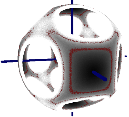
Figure 9: (Color online) Free energy landscape in the variables $c_{1},c_{2},c_{3}$ for system size $\epsilon=0.5$, projected onto a unit sphere. The blue lines indicate the axes ($c_{1}$, etc.) and the red points are contours at $2k_{B}T$ (the square-shaped contour) and $4k_{B}T$ (the stretched contour). The black regions pierced by the axes correspond to the lowest points in the landscape (states with highest entropy).

The phase space of $c_{1},c_{2},c_{3}$ (Eqns. II) has the desired cubical symmetry for our free energy landscape. To generate the landscape, we compile a histogram of the microstates seen in the simulation, $\Omega(c_{1},c_{2},c_{3})$. The entropy is then $S=k_{B}\ln\Omega(c_{1},c_{2},c_{3})$ using Boltzmann’s constant $k_{B}$. The free energy landscape is $F=U-TS=-TS$ (since $U=0$ must be true for non-overlapping hard disks). Equivalently, we can consider $-\ln\Omega$ to be the free energy landscape in units of $k_{B}T$. In this three-dimensional phase space, it turns out that states near the origin are never seen (for $R<4$), so this phase space can be safely projected onto the surface of a unit sphere. This projection is shown in Fig. 9, where the large squarish regions correspond to the equilibrium states, and the tenuous connections through the triangular corner regions show transition paths between the equilibrium states. The empty circular regions correspond to the cube edges, which are configurations that would cause disks to overlap and thus are forbidden.

This is our first free energy landscape. The colors in Fig. 9 indicate the height of the free energy landscape, with darker colors being the minima corresponding to the equilibrium states. To change states, the system must undergo a real-space rearrangement which corresponds to moving from a cube face “up” the energy landscape to one of the corners, and then back “down” to a different cube face; one such trajectory is shown in Fig. 5(f). Given that this is mapped to the surface of a unit sphere, this landscape is a function of only two (angular) coordinates, although given the cubical symmetry it is perhaps more useful to think of this as a function of the three $c$’s which have the proper symmetry. Nonetheless, it is intriguing that the 8 original coordinates can be usefully reduced down to two or three effective coordinates in this free energy landscape.

We now consider a second free energy landscape. Three dot products can be defined as:

$$q_{1} = \vec{v}_{12}\cdot\vec{v}_{34},$$ (3)

$$q_{2} = \vec{v}_{13}\cdot\vec{v}_{42},$$

$$q_{3} = \vec{v}_{14}\cdot\vec{v}_{23}.$$

With these choices, if the four disks are arranged at the corners of a square of side length $s$ such as in Fig. 4, one of the dot products will be zero and the other two will be $\pm s^{2}$. However, states that are reversed are indistinguishable: (1234) is identical to (4321). Thus, rather than six unique states with cubical symmetry, there are three unique states with triangular symmetry. They are $(q_{1},q_{2},q_{3})=(s,-s,0);(-s,0,s);$ and $(0,s,-s)$. In three dimensions, these are the corners of an equilateral triangle. Given that these three points span a plane, we can project the data onto a 2D plane by defining three mutually perpendicular unit vectors:

$$\hat{d_{1}} = (+1,-1,0)/\sqrt{2},$$ (4)

$$\hat{d_{2}} = (+1,+1,-2)/\sqrt{6},$$

$$\hat{d_{3}} = (+1,+1,+1)/\sqrt{3}$$

where $\hat{d_{1}}$ is directed toward the $(s,-s,0)$ location, $\hat{d_{2}}$ is chosen to be in-plane and perpendicular to $\hat{d_{1}}$, and $\hat{d_{3}}=\hat{d_{1}}\times\hat{d_{2}}$. In the plane spanned by $\hat{d_{1}}$ and $\hat{d_{2}}$, we define coordinates by $d_{1}\equiv\hat{d_{1}}\cdot(q_{1},q_{2},q_{3})$, $d_{2}\equiv\hat{d_{2}}\cdot(q_{1},q_{2},q_{3})$. It turns out that $\hat{d_{3}}\cdot(q_{1},q_{2},q_{3})=0$ which can be shown by putting in the definitions of $q_{1},q_{2},q_{3}$ in terms of the original disk positions. This shows that the coordinates $(q_{1},q_{2},q_{3})$ lie on a plane rather than filling a three-dimensional region.

A visualization of the 2D $(d_{1},d_{2})$ free energy landscape is shown in Fig. 10(a). The dark regions are the equilibrium states, and the brighter regions correspond to higher locations on the free energy landscape (lower entropy, and thus the unlikely transition regions). While this representation collapses the six equilibrium states into three minima, nonetheless all transitions are seen in this free energy landscape as landscape trajectories from one local minimum to another one. One such transition is shown in Fig. 5(g).

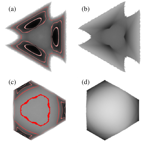
Figure 10: (a) Free energy landscape in $(d_{1},d_{2})$ coordinates for $\epsilon=0.4$. The landscape is bounded by the whitest points. Within the landscape, darker regions are lower (more probable). The red contours are at $1k_{B}T,$ $3k_{B}T$, and $5k_{B}T$. The center of the landscape is a broad local maximum with a height of $4.9k_{B}T$. (b) Map of the effective diffusivity at each point in the landscape. The diffusivity in the center is 1.22 times greater than the diffusivity in the three darker spots. The diffusivity near the long straight outer edges of the landscape is 1.48 times greater than the diffusivity in the darker spots. (c) Free energy landscape in the $(u_{1},u_{2})$ coordinates for $\epsilon=0.4$. The red contours are at $1k_{B}T,$ $3k_{B}T$, $5k_{B}T$, and $7k_{B}T$. The center of the landscape has a height of $7.3k_{B}T$. (d) Map of the effective diffusivity at each point in the landscape. The diffusivity in the center is 2.8 times greater than the diffusivity at the dark edges.

One final free energy landscape that is useful to consider is formed by defining the $q$ variables (Eqns. 3) using unit vectors; that is, changing from $\vec{v}_{12}$ to $\hat{v}_{12}$. The landscape coordinates are then defined using the $\hat{d}$ vectors given in Eqns. 4, leading to coordinates $(u_{1},u_{2})$ in analogy with $(d_{1},d_{2})$. The landscape for these coordinates is shown in Fig. 10(c). Figure 5(h) illustrates a trajectory through this landscape.

Crossings through the exact middle of the phase space [either the $(d_{1},d_{2})$ or ($u_{1},u_{2}$) phase space] correspond to an unusual situation where the transition is equally likely to go to any of three different equilibrium states, as shown in Fig. 6. The disks near the edge of the system become symmetrically placed around the disk in the center, as shown in Fig. 6(d). This arrangement allows the central disk to be equally likely to go to any of the three possible equilibrium states. In the cubical free energy landscape of Fig. 9, this configuration corresponds to the centers of the corners of the cube [Fig. 6(f)], where transitions to any of the adjacent three faces is equally likely.

These three free energy landscape representations (the $c$ variables using the cross products, the $d$ variables using the dot product, and the $u$ variables using the dot product of unit vectors) illustrate our first point about free energy landscapes: Multiple free energy landscapes can be constructed to represent the same system. This point was also made in Ref. hunter12pre , which presented two different one-dimensional landscapes for a system with three hard disks. To an extent this observation is trivial: even the original coordinate system is arbitrary. One could use Cartesian $(x,y)$ coordinates to describe the position of each disk, or polar coordinates $(r,\theta)$. It is reasonable that likewise a free energy landscape could be described by different coordinates.

However, one fact is intriguing: the different representations [Figs. 9 and 10(a,c)] lead to different free energy barrier heights! The barrier heights are plotted in Fig. 11. The free energy barrier heights are similar for the cross products landscape (squares) and the original dot products landscape (triangles), and markedly higher for the unit vector landscape (diamonds). For the first two, it is clear that $\ln(\tau)\sim F_{B}$, that is, the switching time scale grows essentially exponentially with the barrier height. (The deviation from this relationship at large $\epsilon$ is due to the large system size where the disks require more time to diffuse across the system in order to have a transition hunter12pre . That is, as $R$ gets large, the disks spend more time farther apart from one another, and thus the switching time is no longer dominated by the free energy barrier.) The free energy barrier from $(u_{1},u_{2})$ is not only consistently larger than the other two, but also grows faster as $\epsilon\rightarrow 0$ than the other two barriers.

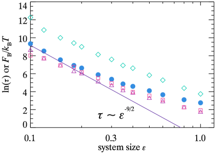
Figure 11: (Color online) The blue circles are $\ln(\tau)$, the log of the switching time scale. The straight line is the same as shown in Fig. 8. The diamonds, squares, and triangles indicate the free energy barrier height for the $u$, $c$, and $d$ free energy landscape variables, respectively. Uncertainties for all points are smaller than the symbol size.

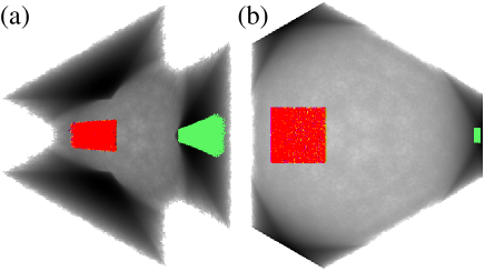
Figure 12: (Color online) Free energy landscapes with $\epsilon=0.2$ for (a) the $(d_{1},d_{2})$ variables and (b) the $(u_{1},u_{2})$ variables. Equivalent points in the two phase spaces are marked by the red regions (left side of both images) and the green regions (right side of both images).

This brings us to our second point about free energy landscapes: The nonlinear mapping used to create free energy landscapes can distort the free energy barrier height. This is especially true when comparing different free energy landscapes. To understand this, consider the mapping from the original 8-dimensional space to a projected free energy landscape. There is some region of the original 8-dimensional space corresponding to the transition states between equilibria with size $\Omega_{t}$, and another region corresponding to the equilibria states of size $\Omega_{e}$. Figure 12 shows that these do not map to equivalent proportions of different landscapes: $\Omega_{t}$ takes up a large portion of the $(u_{1},u_{2})$ landscape and $\Omega_{e}$ takes up a small portion, as seen in Fig. 12(b), large red square and small green rectangle, respectively. However, they map onto nearly equivalent areas in the $(d_{1},d_{2})$ landscape, as seen in Fig. 12(a). For any given small region in the central transition region of Fig. 12(b), there are fewer microstates – the density of microstates per unit area is lower – and thus the entropic barrier $\sim-\ln\Omega$ is higher. Also important is that the density of microstates in the equilibrium region is higher [comparing the green points of Fig. 12(a,b)], thus increasing the entropy associated with those common states for the $(u_{1},u2)$ landscape, which further increases the entropic barrier for the rare transition states.

To be clear, all of these projections are valid and are free energy landscapes for the same system – and the switching time between equilibrium states cannot depend on how we represent the free energy landscape. To understand how the switching time is independent of the free energy landscape, we need to understand how diffusive motion occurs on each landscape. As pointed out by Frenkel frenkel13 , the switching time between two minima is a product of the barrier height and the time it takes to move across the barrier. The latter is based on the barrier width and the diffusion rate across that region. As seen in Fig. 10(a,c) the barrier is much wider for the $(u_{1},u_{2})$ coordinates as well as taller – but also, the system diffuses through this region more quickly. This can be seen by comparing the segment sizes between panels (g) and (h) of Fig. 5. Each segment corresponds to 1000 simulation time steps, and these correspond to larger relative distances in phase space in Fig. 5(h). The combined influence of barrier height, barrier width, and diffusion rate through the transition region are such that the time scale for a transition is the same for all free energy landscapes – as it must be. As it happens, the $(c_{1},c_{2},c_{3})$ and $(d_{1},d_{2})$ landscapes have essentially unchanging crossing attempt rates as $\epsilon\rightarrow 0$ and thus $\ln(\tau)\sim F_{\rm B}$ stays true. This suggests that these two landscape representations are more “useful” to a physicist. To be clear, this discussion has focused on diffusion; similar comments would apply to the ballistic dynamics, where a constant real-space velocity yields different rates of transport in different landscapes.

Effective diffusion rates can vary between landscapes, but the story of diffusion on a free energy landscape is more complicated than that. A third point about free energy landscapes is diffusion rates on the free energy landscape can vary spatially. This is demonstrated in Fig. 10(b,d), which shows the the effective diffusivity at each point in the landscapes corresponding to panels (a,c). The effective diffusivity was determined by simulating the system for a long time ($>100$ transitions). At each time we save the position that the system is at in the landscape, and then measure how much that position changes in the next simulation time step. The effective diffusion is measured as the mean square landscape displacement, as a function of the initial coordinate. Recall that at each time step, disks can move a distance $10^{-2.5}$ in any direction in real space: this is always the same no matter where the disk is, with the exception of configurations where that movement is disallowed so that overlaps are avoided. In the landscape, however, the motion depends on the transformation from the 8 real space coordinates into the landscape coordinates, and this is nonlinear. The real space motions result in a smaller or larger movement within the landscape depending on the position, as Fig. 10(b,d) demonstrates. For example, if all four disks are far from each other, then slight real-space motions change their relative angles $\theta$ by small amounts. Recall that cross products such as Eqns. II are related to $\sin\theta$ and dot products such as Eqns. 4 are related to $\cos\theta$, so thus regions of the landscape corresponding to disks far apart in real space have smaller changes in $\theta$ and therefore have slower landscape motion. Again, while this discussion is considering diffusive dynamics, similar comments hold for ballistic dynamics: a constant real-space velocity leads to a non-constant velocity through a landscape.

IV Quantifying the entropic barrier

Returning to the question of the power-law dependence of the switching time scale $\tau$ on $\epsilon$ seen in Fig. 8, we can understand this by recognizing it is an entropic barrier. Following Ref. hunter12pre , the barrier can be quantified by counting the number of microstates $\Omega_{t}$ available at a transition. A transition involves three collinear disks: the center disk is the one passing between the other two, thus defining a swap, see for example Fig. 5(c,d). If this line is along a diameter of the system, then the relative positions of each of those three disks are described by just three coordinates. The length of the diameter is $6+2\epsilon$, but as each disk has a diameter of length 2, the amount of free space is $2\epsilon$. If one disk was confined to this much free space, then $\Omega_{t}=2\epsilon$. For the three disks, while they must share this free space, they each have $O(\epsilon)$ possible positions and thus $\Omega_{t}\sim\epsilon^{3}$ for the three of them; this can be confirmed by an exact calculation hunter12pre . However, transitions can occur when the disks are along a line other than the diameter, so long as that line is at least of length $6$. The position of that line has $O(\epsilon^{1/2})$ possibilities, giving $\Omega_{t}\sim\epsilon^{7/2}$ for three disks to make a transition hunter12pre . The fourth disk, which is not as involved in the transition, nonetheless needs to be out of the center of the system: the number of microstates corresponding to this extra degree of freedom is also proportional to $\epsilon$, leading to the overall $\Omega_{t}\sim\epsilon^{9/2}$.

Compared to this transition state, the number of microstates $\Omega_{e}$ associated with the equilibrium states is quite large, and essentially independent of $\epsilon$ when $\epsilon\ll 1$. Therefore growth of the entropic barrier as $\epsilon\rightarrow 0$ is determined by the $\epsilon$ dependence of $\Omega_{t}$ (related to the transition state). This argument then suggests an entropic barrier that grows as $F_{\rm B}/k_{B}T=-S_{\rm B}T/k_{B}T\sim-\ln\Omega_{t}\sim\ln\epsilon^{-9/2}$. In other words, the system has to find one of the rare transition microstates counted by $\Omega$ as opposed to being in the many microstates associated with a common configuration. The scarcity of the transition microstates as $\epsilon$ becomes small is what increases the entropic barrier, and thus slows down the transition. There is also a time scale $\tau_{0}$ for attempts to cross the barrier, such that $\tau=\tau_{0}\exp(F_{B}/k_{B}T)\sim\tau_{0}\epsilon^{-9/2}$. Figure 8 shows this relation holds as $\epsilon\rightarrow 0$. Note that this argument of counting the microstates does not depend on defining a free energy landscape. Rather, this is a direct counting of microstates in the original 8 dimensional state space, and thus does not have any of the arbitrariness of defining new coordinates.

V Conclusions

We have presented a simple model system comprised of four disks moving in a small region. This system can be described by several different free energy landscapes, with greater or lesser success. The spherical representation shown in Fig. 9 has the advantage of emphasizing the symmetry of the landscape and the existence of six unique local minima. However, it has the drawback of requiring a 3D representation, and thus is slightly harder to depict on the printed page. The simpler triangular landscape of Fig. 10(a) collapses the six minima into three, with the gained advantage of a purely 2D representation. A different version of this triangular landscape, shown in Fig. 10(c), has the disadvantage that the apparent free energy barrier height is not as useful for determining the transition rate between states. These three landscapes illustrate the main points we have made about free energy landscapes: (a) a system does not have “the” free energy landscape, but rather multiple free energy landscapes can be defined for a given system; (b) different free energy landscapes have different apparent barrier heights; (c) the different apparent barrier heights are compensated for by different effective diffusivity rates on different landscapes, such that the transition rate between states is independent of choice of free energy landscape description. A related point is that the effective diffusivity rate depends on the location in the free energy landscape. For well-chosen free energy landscapes and in the limit of small system size, the transition time scale between states has an Arrhenius scaling depending on the free energy barrier height. For simulations with ballistic dynamics, the conclusions about diffusivity map smoothly to conclusions about speed of trajectories through the different landscapes.

One additional point can be made by comparing this four disk model with an earlier three disk model hunter12pre . The earlier model has free energy landscapes describable by only one coordinate, for example $\vec{v}_{12}\times\vec{v}_{13}$ (compare with our Eqn. II). By adding one disk, we need to add at least one coordinate in a useful free energy landscape description. Clearly as we increase the number of disks (or consider spheres moving in three dimensions) we will need more coordinates for a free energy landscape description. It seems likely that the number of needed coordinates will scale as the number of particles $N$ for large $N$, but exactly how this scaling should behave for large $N$ is unclear. Nonetheless, it suggests that one can imagine that a free energy landscape for $N\gg 1$ can be described by some space with a dimensionality lower than the original coordinate space, and the landscape will be highly symmetric albeit in some number of dimensions hard to visualize. It is plausible that explicitly constructed free energy landscapes for large systems may be of limited use given that they are still high-dimensional, as is the original potential energy landscape. Nonetheless we note that often authors do think about free energy landscapes for hard particle systems (e.g., bowles06 ; ashwin09 ; carlsson12 ; holmescerfon13 ; charbonneau14 ) so it is encouraging to think that such landscapes could, at least hypothetically, be constructed in a manner such as we have done in this work.

A final comment is that if the particles in a system are not hard, but interact with some interaction potential, then the potential energy term $U$ contributes also to the free energy. This situation is considered elsewhere in the context of the earlier three disk model du16 , which found that the entropic and energetic contributions to the free energy landscape are often comparable. That is, transitions can require both a thermal fluctuation that allows particles to interact more strongly and increase $U$, and also that particles find a rare, low entropy state. Nonetheless, the main points listed above for free energy landscapes will still be true for situations with nontrivial potential energy.

We thank G. L. Hunter for helpful discussions. This work was supported by the National Science Foundation (CBET-1336401 and CBET-1804186).

References

- (1) M. Goldstein. “Viscous liquids and the glass transition: A potential energy barrier picture.” J. Chem. Phys., 51, 3728–3739 (1969).
- (2) F. Sciortino & P. Tartaglia. “Glassy colloidal systems.” Adv. Phys., 54, 471–524 (2005).
- (3) V. K. de Souza & D. J. Wales. “Energy landscapes for diffusion: Analysis of cage-breaking processes.” J. Chem. Phys., 129, 164507 (2008).
- (4) J. D. Bryngelson, J. N. Onuchic, N. D. Socci, & P. G. Wolynes. “Funnels, pathways, and the energy landscape of protein folding: A synthesis.” Proteins: Structure, Function, and Bioinformatics, 21, 167–195 (1995).
- (5) R. S. Berry, N. Elmaci, J. P. Rose, & B. Vekhter. “Linking topography of its potential surface with the dynamics of folding of a protein model.” Proc. Nat. Acad. Sci., 94, 9520–9524 (1997).
- (6) J. A. Joseph, K. Röder, D. Chakraborty, R. G. Mantell, & D. J. Wales. “Exploring biomolecular energy landscapes.” Chem. Comm., 53, 6974–6988 (2017).
- (7) R. Marcelin. “Expression des vitesses de transformation des systèmes physico-chimiques en fonction de l’affinité.” Compt. Rend. Hebd. Seances Acad. Sci., 158, 116–118 (1914).
- (8) S. Awasthi & N. N. Nair. “Exploring high-dimensional free energy landscapes of chemical reactions.” WIREs Comput. Mol. Sci., 9, e1398 (2019).
- (9) F. Krzakala & J. Kurchan. “Landscape analysis of constraint satisfaction problems.” Physical Review E, 76, 021122 (2007).
- (10) A. J. Ballard, R. Das, S. Martiniani, D. Mehta, L. Sagun, J. D. Stevenson, & D. J. Wales. “Energy landscapes for machine learning.” Phys. Chem. Chem. Phys., 19, 12585–12603 (2017).
- (11) K. J. Laidler. “Rene Marcelin (1885-1914), a short-lived genius of chemical kinetics.” J. Chem. Educ., 62, 1012 (1985).
- (12) F. H. Stillinger & T. A. Weber. “Packing structures and transitions in liquids and solids.” Science, 225, 983–989 (1984).
- (13) F. H. Stillinger. “Supercooled liquids, glass transitions, and the Kauzmann paradox.” J. Chem. Phys., 88, 7818–7825 (1988).
- (14) F. H. Stillinger. “A topographic view of supercooled liquids and glass formation.” Science, 267, 1935–1939 (1995).
- (15) B. J. Alder & T. E. Wainwright. “Phase transition for a hard sphere system.” J. Chem. Phys., 27, 1208–1209 (1957).
- (16) W. W. Wood & J. D. Jacobson. “Preliminary results from a recalculation of the Monte Carlo equation of state of hard spheres.” J. Chem. Phys., 27, 1207–1208 (1957).
- (17) J. D. Bernal. “The Bakerian lecture, 1962. The structure of liquids.” Proc. Roy. Soc. London. Series A, 280, 299–322 (1964).
- (18) B. Widom. “Intermolecular forces and the nature of the liquid state.” Science, 157, 375–382 (1967).
- (19) P. N. Pusey & W. van Megen. “Phase behaviour of concentrated suspensions of nearly hard colloidal spheres.” Nature, 320, 340–342 (1986).
- (20) H. X. Zhou & R. Zwanzig. “A rate process with an entropy barrier.” J. Chem. Phys., 94, 6147–6152 (1991).
- (21) G. L. Hunter & E. R. Weeks. “Free-energy landscape for cage breaking of three hard disks.” Phys. Rev. E, 85, 031504 (2012).
- (22) T. L. Hill & E. Eisenberg. “Reaction free energy surfaces in myosin-actin-ATP systems.” Biochemistry, 15, 1629–1635 (1976).
- (23) C. M. Soukoulis, K. Levin, & G. S. Grest. “Reversibility and Irreversibility in Spin-Glasses: The Free-Energy Surface.” Phys. Rev. Lett., 48, 1756–1759 (1982).
- (24) G. H. Paine & H. A. Scheraga. “Prediction of the native conformation of a polypeptide by a statistical-mechanical procedure. I. Backbone structure of enkephalin.” Biopolymers, 24, 1391–1436 (1985).
- (25) W. Fontana, T. Griesmacher, W. Schnabl, P. F. Stadler, & P. Schuster. “Statistics of landscapes based on free energies, replication and degradation rate constants of RNA secondary structures.” Monatshefte für Chemie, 122, 795–819 (1991).
- (26) D. Wales. Energy Landscapes: Applications to Clusters, Biomolecule s and Glasses. Cambridge Molecular Science (Cambridge University Press, Cambridge) (2004). ISBN 978-0-521-81415-7.
- (27) D. J. Wales & T. V. Bogdan. “Potential energy and free energy landscapes.” J. Phys. Chem. B, 110, 20765–20776 (2006).
- (28) S. P. Giarritta & P. V. Giaquinta. “Statistical geometry of four calottes on a sphere.” J. Stat. Phys., 75, 1093–1118 (1994).
- (29) R. J. Speedy. “Two disks in a box.” Physica A: Statistical Mechanics and its Applications, 210, 341–351 (1994).
- (30) R. K. Bowles & R. J. Speedy. “Five discs in a box.” Physica A, 262, 76–87 (1999).
- (31) R. K. Bowles & I. Saika-Voivod. “Landscapes, dynamic heterogeneity, and kinetic facilitation in a simple off-lattice model.” Phys. Rev. E, 73, 011503 (2006).
- (32) S. S. Ashwin & R. K. Bowles. “Complete jamming landscape of confined hard discs.” Phys. Rev. Lett., 102, 235701 (2009).
- (33) G. Carlsson, J. Gorham, M. Kahle, & J. Mason. “Computational topology for configuration spaces of hard disks.” Phys. Rev. E, 85, 011303 (2012).
- (34) M. Barnett-Jones, P. A. Dickinson, M. J. Godfrey, T. Grundy, & M. A. Moore. “Transition state theory and the dynamics of hard disks.” Phys. Rev. E, 88, 052132 (2013).
- (35) P. Hinow. “A nonsmooth program for jamming hard spheres.” Optim. Lett., 8, 13–33 (2014).
- (36) M. J. Godfrey & M. A. Moore. “Static and dynamical properties of a hard-disk fluid confined to a narrow channel.” Phys. Rev. E, 89, 032111 (2014).
- (37) M. J. Godfrey & M. A. Moore. “Understanding the ideal glass transition: Lessons from an equilibrium study of hard disks in a channel.” Phys. Rev. E, 91 (2015).
- (38) J. F. Robinson, M. J. Godfrey, & M. A. Moore. “Glasslike behavior of a hard-disk fluid confined to a narrow channel.” Phys. Rev. E, 93 (2016).
- (39) M. D. Ediger & P. Harrowell. “Perspective: Supercooled liquids and glasses.” J. Chem. Phys., 137, 080901 (2012).
- (40) G. Biroli & J. P. Garrahan. “Perspective: The glass transition.” J. Chem. Phys., 138, 12A301 (2013).
- (41) C. Donati, J. F. Douglas, W. Kob, S. J. Plimpton, P. H. Poole, & S. C. Glotzer. “Stringlike cooperative motion in a supercooled liquid.” Phys. Rev. Lett., 80, 2338–2341 (1998).
- (42) B. Doliwa & A. Heuer. “Cooperativity and spatial correlations near the glass transition: Computer simulation results for hard spheres and disks.” Phys. Rev. E, 61, 6898–6908 (2000).
- (43) D. Frenkel. “Simulations: The dark side.” Euro. Phys. J. Plus, 128, 1–21 (2013).
- (44) M. Holmes-Cerfon, S. J. Gortler, & M. P. Brenner. “A geometrical approach to computing free-energy landscapes from short-ranged potentials.” Proc. Nat. Acad. Sci., 110, E5–E14 (2013).
- (45) P. Charbonneau, J. Kurchan, G. Parisi, P. Urbani, & F. Zamponi. “Fractal free energy landscapes in structural glasses.” Nature Comm., 5, 4725 (2014).
- (46) X. Du & E. R. Weeks. “Energy barriers, entropy barriers, and non-Arrhenius behavior in a minimal glassy model.” Phys. Rev. E, 93, 062613 (2016).