Revisit on holographic complexity in two-dimensional gravity

Abstract

We revisit the late-time growth rate of various holographic complexity conjectures for neutral and charged AdS black holes with single or multiple horizons in two dimensional (2D) gravity like Jackiw-Teitelboim (JT) gravity and JT-like gravity. For complexity-action conjecture, we propose an alternative resolution to the vanishing growth rate at late-time for general 2D neutral black hole with multiple horizons as found in the previous studies for JT gravity. For complexity-volume conjectures, we obtain the generic forms of late-time growth rates in the context of extremal volume and Wheeler-DeWitt volume by appropriately accounting for the black hole thermodynamics in 2D gravity.

1 Introduction

Despite the role as the earliest discovered fundamental interaction, gravity still remains as a myth by its quantum nature. General relativity reveals gravity as the manifestation of background geometry, and Ryu-Takayanagi formula Ryu:2006bv motivates the pursuit of bulk geometry as a dual to some quantum information on the boundary, then a natural question to ask is whether gravity in the bulk could be reconstructed from quantum information on the boundary. This triangular relation between gravity, geometry and information is the main focus recently among the high-energy physics communities.

In the context of an eternal anti-de Sitter (AdS) black hole, quantum information on the boundary could be extracted from the dubbed thermo-field double (TFD) state Maldacena:2001kr . However, entanglement entropy alone cannot capture all the quantum information on the boundary Hartman:2013qma ; Susskind:2014moa , nor can bulk geometry be fully reconstructed from the entanglement entropy alone Freivogel:2014lja , hence there comes the need for complexity, which continues to growth even after reaching thermal equilibrium, similar to the growth of black hole interior. This holographic insight was first formulated in the context of complexity-volume (CV) conjecture Susskind:2014rva ; Stanford:2014jda (see also Couch:2016exn ; Couch:2018phr for other CV proposals) and later refined in the context of complexity-action (CA) conjecture Brown:2015bva ; Brown:2015lvg (see also Hayward:1993my ; Brill:1994mb ; Lehner:2016vdi ; Ruan:2017tkr for the clarification of action computation).

Although there have been extensive studies on CV and CA conjectures from the bulk side (see, e.g. charged black holes Cai:2016xho ; Cai:2017sjv , UV divergences Chapman:2016hwi ; Reynolds:2016rvl ; Carmi:2016wjl ; Kim:2017lrw , subregion complexity Carmi:2016wjl ; Ben-Ami:2016qex ; Abt:2017pmf , time-evolution Brown:2017jil ; Carmi:2017jqz , higher derivative gravities Cai:2016xho ; Alishahiha:2017hwg ; Cano:2018aqi , Einstein-Maxwell-dilaton gravities Cai:2017sjv ; Swingle:2017zcd ; An:2018xhv ; Alishahiha:2018tep , Vaidya spacetimes Chapman:2018dem ; Chapman:2018lsv , switchback effect and quenches Susskind:2014jwa ; Moosa:2017yvt , and dS/FLRW boundaries Reynolds:2017lwq ; An:2019opz ), the difficulty to establish a convincing holographic complexity lies in the lack of unique and well-defined notion for the complexity in the field theory from the boundary side Roberts:2016hpo ; Hashimoto:2017fga ; Kim:2017qrq ; Chapman:2017rqy ; Czech:2017ryf ; Jefferson:2017sdb ; Caputa:2017urj ; Caputa:2017yrh ; Bhattacharyya:2018bbv ; Belin:2018bpg ; Ali:2018fcz ; Belin:2018fxe ; Chapman:2018hou ; Balasubramanian:2018hsu ; Caputa:2018kdj ; Guo:2018kzl ; Yang:2018nda ; Takayanagi:2018pml ; Hackl:2018ptj ; Khan:2018rzm ; Yang:2018tpo ; Bhattacharyya:2018wym ; Camargo:2019isp ; Bhattacharyya:2019kvj ; Doroudiani:2019llj ; Yang:2019udi ; Sinamuli:2019utz ; Caceres:2019pgf . Note that the Lloyd bound Lloyd on complexity growth rate was initially founded in quantum mechanical system, it makes the two-dimensional (2D) gravity Muta:1992xw ; Nojiri:2000ja ; Grumiller:2002nm be a special case to understand holographic complexity since the boundary theory could be a (super)conformal quantum mechanics (CQM) Chamon:2011xk .

Despite the fact that the AdS₂/CFT₁ is currently poor understood Castro:2008ms ; Cvetic:2016eiv , the renewed interest on 2D gravity follows up the recent understanding Polchinski:2016xgd ; Maldacena:2016hyu of Sachdev-Ye-Kitaev (SYK) model Sachdev:1992fk ; KitaevTalks , which is conjectured to be dual to quantum gravity in two dimensions Jensen:2016pah ; Engelsoy:2016xyb . As a toy model of the correspondences between bulk 2D gravity Strominger:1998yg and boundary quantum mechanics (QM) Claus:1998ts , the 2D AdS Jackiw-Teitelboim(JT) gravity Jackiw:1982hg ; Teitelboim:1983fg is found in Cadoni:2000gm to be dual to a conformally invariant dynamics on the spacetime boundary that could be described in terms of a de Alfaro-Fubini-Furlan model deAlfaro:1976vlx coupled to an external source with conformal dimension two. Later in Brigante:2002rv , the asymptotic dynamics of 2D (A)dS JT gravity is further found to be dual to a generalized two-particle Calogero-Sutherland quantum mechanical model Sutherland:1971kq ; Gibbons:1998fa . Based on JT model, the Almheiri-Polchinski (AP) model Almheiri:2014cka was recently introduced to study the back-reaction to AdS₂ since there are no finite energy excitations above the AdS₂ vacuum Fiola:1994ir ; Maldacena:1998uz . A distinct feature of AP model is that the boundary time coordinate is lifted as a dynamical variable and could be described by the 1D Schwarzian derivative action Maldacena:2016upp ; Engelsoy:2016xyb , of which the same pattern of action also appeares in the SYK model. This indicates that JT model might arise as a holographic description of infrared limit of SYK model.

The issue of holographic complexity for 2D JT gravity has been investigated in Brown:2018bms ; Akhavan:2018wla ; Alishahiha:2018swh ; Goto:2018iay . Naive computations of action growth rate for 2D JT gravity reduced from a near-extremal and near-horizon limit of Reissner-Nordstr$\ddot{\text{o}}$m (RN) black holes in higher dimensions was found to be perplexingly vanishing at late-time, of which, however, the late-time linear growth of the complexity could be restored by appending with an electromagnetic boundary term Brown:2018bms in order to ensure the correct sign of the dilaton potential during dimensional reduction. Akhavan:2018wla ; Alishahiha:2018swh proposed another restoration of the late-time linear growth of the complexity by appropriately relating the cut-off behind the horizon with the UV cut-off at the boundary (see also Hashemi:2019xeq ). Recently, Goto:2018iay revealed an intriguing fact that the action growth rate for charged black hole is sensitive to the ratio between the electric and magnetic charges, and the previously identified vanishing result is due to the zero electric charged in the grand canonical ensemble, which could be dramatically changed by adding an appropriate surface term. In this paper, we would like to go beyond the 2D JT gravity.

We investigated the late-time growth rate for neutral and charged asymptotically $\text{AdS}_{2}$ dilaton black hole solutions with single or multiple horizons in two dimensional (2D) gravity like Jackiw-Teitelboim (JT) gravity and JT-like gravity, by suing the CA and CV conjectures. The main results are briefly summarized briefly: i) In the case with CA conjecture, for charged black holes with single or multiple horizons and neutral black holes with single horizon, the late-time growth rate of complexity exactly saturates the charged or neutral versions of Lloyd bound, respectively. In particular, for neutral black hole with multiple horizons, the late-time growth rate is found to be vanished if the conventional approach is naively adopted. To resolve this puzzle, we make use of magnetic/electrical duality of 4D RN AdS black hole to restore the late-time linear growth of complexity, which can be regarded as a generalization of the method introduced in Brown:2018bms . ii) In the CV1.0 conjecture, the universal form of late-time growth rate is obtained for generic neutral and charged asymptotically $\text{AdS}_{2}$ dilaton black hole solutions with single or multiple horizons. In the CV 2.0 version, we obtain the generic forms of late-time growth rates in the context of Wheeler-de Witt volume by appropriately accounting for the 2D black hole thermodynamics.

The organization of the remaining parts of this paper is as follows. The holographic complexity in terms of CA, CV 1.0 as well as CV 2.0, in 2D neutral and charged black holes have been investigated in Sec. 2, Sec. 3 and Sec. 4, respectively. Sec. 5 is devoted to conclusions. The appendix A elaborates the form of counter term and topological term for the 2D black holes.

2 CA

In this section, we evaluate the late-time growth rate of holographic complexity for neutral and charged eternal $\text{AdS}_{2}$ black holes using the CA conjecture, which claims that the complexity of a TFD state living on the boundaries is proportional to the gravitational action evaluated on the Wheeler-DeWitt (WDW) patch

$$\mathcal{C_{A}}=\frac{\mathcal{A}_{\mathrm{WDW}}}{\pi\hbar}.$$ (1)

Here the coefficient $1/\pi\hbar$ is chosen in such a way that the late-time limit $t\equiv t_{L}+t_{R}\to\infty$ of $\mathcal{C_{A}}$ growth rate exactly saturates the Lloyd bound Lloyd

$$\left.\frac{\mathrm{d}\mathcal{C_{A}}}{\mathrm{d}t}\right|_{t\to\infty}=\frac{2M}{\pi\hbar}$$ (2)

at least for AdS Schwarzschild black hole in $D\geq 4$ dimensions in Einstein gravity Brown:2015lvg , beyond which various corrections to $2M$ at late-time are expected for other neutral AdS black holes also with a single horizon. However, for charged AdS black holes with both inner and outer horizons, the holographic complexity given by CA conjecture saturates at late-time a different form Cai:2016xho as

$$\left.\frac{\mathrm{d}\mathcal{C_{A}}}{\mathrm{d}t}\right|_{t\to\infty}=\frac{1}{\pi\hbar}(M-\mu Q-\Omega J)\bigg{|}_{r_{-}}^{r_{+}},$$ (3)

where the inner horizon $r_{-}$ emerges besides the outermost horizon $r_{+}$ due to the presence of conserved charges $Q$ and $J$ with corresponding chemical potentials $\mu$ and $\Omega$, respectively. The form (3) (see also Huang:2016fks ; Liu:2019mxz ) is quite generic for charged AdS black holes with double horizons even beyond the Einstein gravity. Nevertheless, there also exists other special cases of neutral black holes with multiple horizons and charged black holes with a single horizon (for example, see Cai:2017sjv ). All these cases mentioned above will be studied below for 2D AdS black holes beyond simple JT gravity.

2.1 Neutral black holes

We start with the neutral AdS black holes in 2D gravity with Einstein-Hilbert-dilaton action of form

$$\mathcal{A}[g,\phi]=\frac{1}{2G}\int_{\mathcal{M}}\mathrm{d}^{2}x\sqrt{-g}\left(\phi R(g)+\frac{V(\phi)}{L^{2}}\right)+\frac{1}{G}\int_{\partial\mathcal{M}}\mathrm{d}x\sqrt{-h}\Big{(}\phi K-\mathcal{L}_{\mathrm{ct}}^{\mathrm{neu}}(\phi)\Big{)},$$ (4)

where $\mathcal{L}_{\mathrm{ct}}^{\mathrm{neu}}$ is a boundary counter term that renders the Euclidean on-shell action finite. With the ansatz of a linear dilaton of mass scale $\alpha$ and Schwarzschild gauge of the metric

$$\phi =\alpha r,$$ (5)

$$\mathrm{d}s^{2} =-f(\phi)\mathrm{d}t^{2}+f(\phi)^{-1}\mathrm{d}r^{2},$$ (6)

the corresponding equations-of-motion (EOMs)

$$R =-\frac{V^{\prime}(\phi)}{L^{2}},$$ (7)

$$0 =-\nabla_{\mu}\nabla_{\nu}\phi+g_{\mu\nu}\left(\nabla^{2}\phi-\frac{V(\phi)}{2L^{2}}\right)$$ (8)

could be solved as

$$f(\phi) =-\frac{2GM}{\alpha}+j(\phi),$$ (9)

$$j(\phi) =\frac{1}{\alpha^{2}L^{2}}\int^{\phi}V(\phi^{\prime})d\phi^{\prime},$$ (10)

where $M$ is the ADM mass as shown in Appendix A in order to preserve the thermodynamic relation with the black hole temperature and Wald entropy Wald:1993nt defined respectively by

$$T =\frac{f^{\prime}(r_{+})}{4\pi}=\frac{V(\phi_{+})}{4\pi\alpha L^{2}},$$ (11)

$$S =\frac{2\pi\phi_{+}}{G},\quad\phi_{+}\equiv\alpha r_{+}.$$ (12)

The boundary term is therefore computed by

$$\sqrt{-h}K =\frac{V(\phi)}{2\alpha L^{2}}.$$ (13)

$$\mathcal{L}_{\mathrm{ct}}^{\mathrm{neu}} =\alpha\sqrt{j(\phi)},$$ (14)

One could refer to (14) in Appendix A for more details.

We next turn to a particular form of potential motivated by Kettner:2004aw

$$V(\phi)=2\phi+B+\sum\limits_{i}B_{i}\phi^{b_{i}},\quad b_{i}\neq 0,1$$ (15)

which becomes JT gravity when $B=B_{i}=0$. The corresponding on-shell Ricci scalar curvature $R$ is

$$R=-\alpha^{2}f^{\prime\prime}(\phi)=-\frac{2}{L^{2}}+\sum_{i}b_{i}B_{i}\phi^{b_{i}-1},$$ (16)

where a curvature singularity would appear at $r=0$ when there is a nonzero $B_{i}$. What’s more, one should restrict $b_{i}<1$ to obtain an asymptotically $\mathrm{AdS}_{2}$ geometry. Based on above arguments, the black hole solutions generated by (15) could be divided into two classes: the one with single horizon and the one with multiple horizons, which will be studied in detail below.

2.1.1 Single horizon

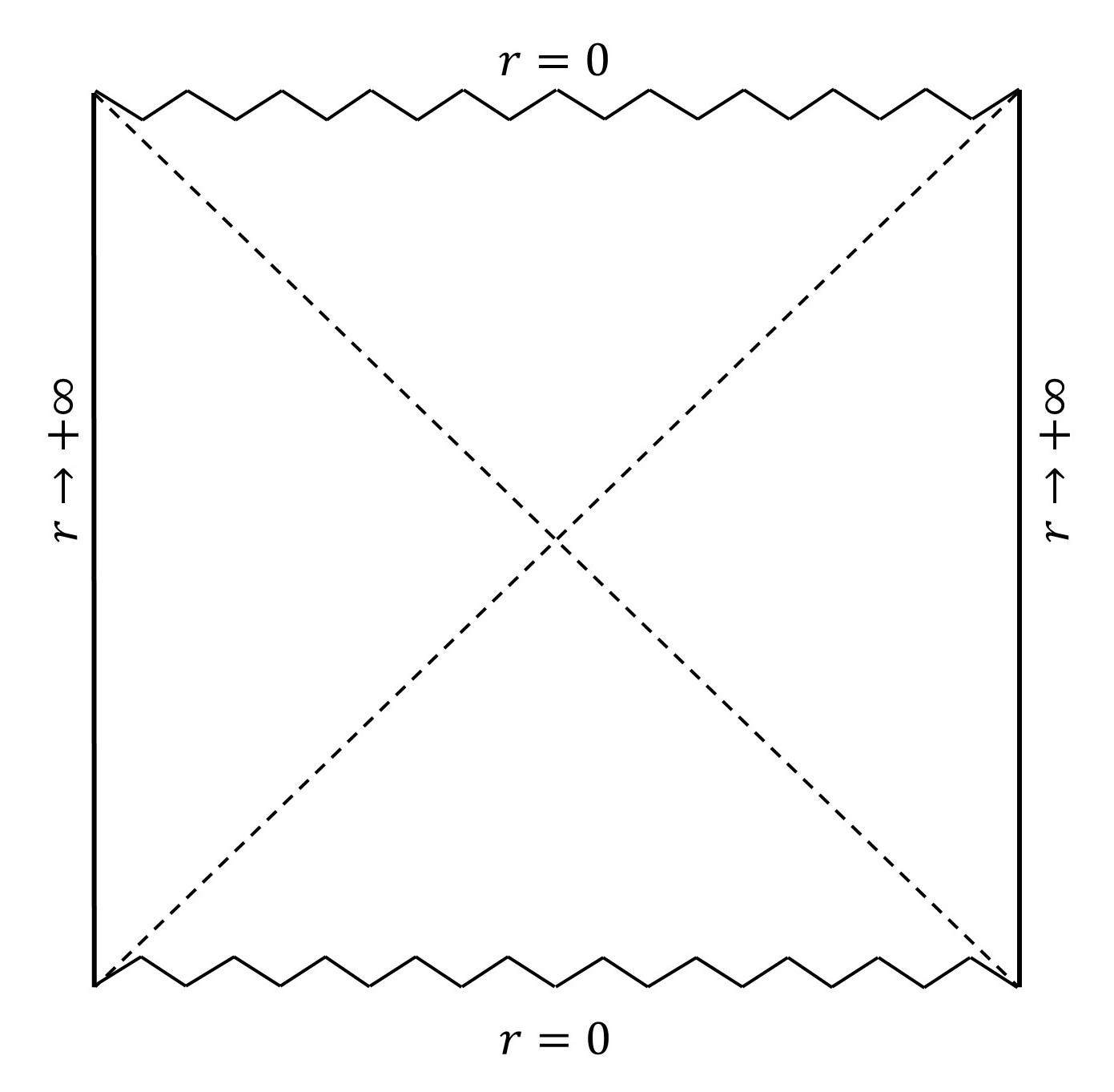
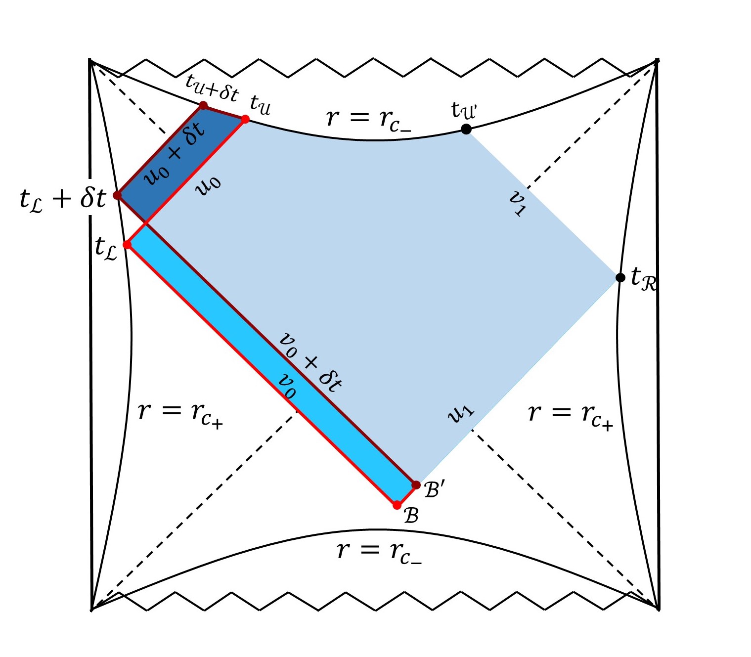
Figure 1: Left panel: Neutral (Charged) AdS black hole in 2D gravity with a single horizon at $r=r_{h}$ (dashed lines), spatial singularities at $r=0$ (wavy lines) and asymptotic boundaries at $r\to\infty$ (vertical lines). Right panel: The change of WDW patches from the one anchored on $t_{L}$ and $t_{R}$ (pale blue and bright blue regions) to the one anchored on $t_{L}+\delta t$ and $t_{R}$ (pale blue and dark blue regions). The UV and IR cutoffs are placed at $r=r_{c_{+}}$ and $r=r_{c_{-}}$, respectively.

If there is a nonzero $B_{i}$, then the non-extreme single horizon solutions are allowed, namely, $f(\phi)=0$ has one positive root, of which the Penrose diagrams share the same feature as shown in Fig.1. Without lost of generality, the left and right boundaries could be related to the Schwarzschild time by $t_{L}=t,t_{R}=-t$, and the Eddington-Finkelstein coordinates $u=t+r^{*}$ and $v=t-r^{*}$ with $r^{*}=\int f(r)^{-1}\mathrm{d}r$ and $\rho(r^{*}(r))=r$ are introduced to rewrite the metric as $\mathrm{d}s^{2}=-f(r)\mathrm{d}u^{2}+2\mathrm{d}u\mathrm{d}r=-f(r)\mathrm{d}v^{2}-2\mathrm{d}v\mathrm{d}r$.

Following the convention of Lehner:2016vdi , the total change of action due to changing the WDW patch reads

$$\delta\mathcal{A}_{\text{WDW}}=\delta\mathcal{A}^{\text{WDW}}_{\text{bulk}}+\delta\mathcal{A}^{\text{WDW}}_{\text{ren.}\text{surf}}+\delta\mathcal{A}^{\text{WDW}}_{\text{joint}},$$ (17)

where $\mathcal{A}^{\text{WDW}}_{\text{ren.}\text{surf}}$ is the surface term we renormalized to make the late-time action growth rate converge,

$$A^{\text{WDW}}_{\text{ren.surf}}=\int_{r=r_{c_{-}}\bigcap\text{WDW}{\text{patch}}}\sqrt{|h|}\mathrm{d}t\Big{(}\phi K-\frac{\alpha j(\phi)}{\sqrt{|f(\phi)|}}\Big{)}.$$ (18)

The bulk term contribution is

$$\delta\mathcal{A}^{\text{WDW}}_{\text{bulk}} =\frac{1}{2G}\int^{u_{0}+\delta t}_{u_{0}}\mathrm{d}u\int_{r_{c_{-}}}^{\rho\big{(}\frac{u-(v_{0}+\delta t)}{2}\big{)}}\frac{V(\phi)-\phi V^{\prime}(\phi)}{L^{2}}\mathrm{d}r$$

$$-\frac{1}{2G}\int_{v_{0}}^{v_{0}+\delta t}\mathrm{d}v\int_{\rho\big{(}\frac{u_{1}-v}{2}\big{)}}^{\rho\big{(}\frac{u_{0}-v}{2}\big{)}}\frac{V(\phi)-\phi V^{\prime}(\phi)}{L^{2}}\mathrm{d}r$$

$$=\delta t\Big{(}\frac{\alpha j(\phi)}{G}-\frac{\phi V(\phi)}{2G\alpha L^{2}}\Big{)}\bigg{|}^{\phi_{\mathcal{B}}}_{\phi_{c_{-}}},$$ (19)

the contribution of the renormalised-surface term is

$$\delta\mathcal{A}^{\text{WDW}}_{\text{ren.}\text{surf}} =-\frac{1}{G}\int_{u_{0}-r^{*}(r_{c_{-}})}^{u_{0}-r^{*}(r_{c_{-}})+\delta t}\sqrt{|h|}\mathrm{d}t\Big{(}\phi K-\frac{\alpha j(\phi)}{\sqrt{|f(\phi)|}}\Big{)}$$

$$=\delta t\Big{(}-\frac{\phi V(\phi)}{2G\alpha L^{2}}+\frac{\alpha j(\phi)}{G}\Big{)}\bigg{|}_{\phi=\phi_{c_{-}}},$$ (20)

and the joint term contribution is

$$\delta\mathcal{A}^{\text{WDW}}_{\text{joint}} =\frac{1}{G}\phi_{\mathcal{B}^{\prime}}a_{\mathcal{B}^{\prime}}-\frac{1}{G}\phi_{\mathcal{B}}a_{\mathcal{B}}$$

$$=\delta t\bigg{(}\frac{\phi V(\phi)}{2G\alpha L^{2}}+\frac{\alpha f(\phi)}{2G}\log\Big{|}\frac{f(\phi)}{c\bar{c}}\Big{|}\bigg{)}\bigg{|}_{\phi=\phi_{\mathcal{B}}},$$ (21)

then the total variation of $\mathcal{A}_{\text{WDW}}$ is

$$\delta\mathcal{A}_{\text{WDW}}=\delta t\Big{(}\frac{\alpha j(\phi)}{G}+\frac{\alpha f(\phi)}{2G}\log\Big{|}\frac{f(\phi)}{c\bar{c}}\Big{|}\Big{)}\bigg{|}_{\phi=\phi_{\mathcal{B}}}.$$ (22)

As the boundary time goes to infinity, $\phi_{\mathcal{B}}\rightarrow\phi_{h}$, then we have

$$\frac{\mathrm{d}\mathcal{A}_{\text{WDW}}}{\mathrm{d}t}\bigg{|}_{t\rightarrow+\infty}=2M,$$ (23)

which is the same as that of Schwartzchild-AdS black hole in higher dimensional gravity Brown:2015lvg . Note that the extra boundary counter term we introduced in (20) not only offsets the possible divergence, but also makes the action growth rate saturate the desired Lloyd bound. It’s also important to point out that the form of the additional counter term is not uniquely fixed.

Finally, the rate (2.23) only depends on the mass. To see how the rate depends on the entropy, one can rewrite $M$ as a function of entropy $S$ and temperature $T$ which are determined by the black hole horizon $r_{+}$, that is

$$M=ST\Big{(}\frac{\int^{\phi_{+}}V(\phi)\mathrm{d}\phi}{\phi_{+}V(\phi_{+})}\Big{)}\Big{|}_{\phi_{+}=\frac{GS}{2\pi}}.$$ (24)

For generic form of the dilaton potential (2.15), the result is

$$M=ST\cdot\frac{1+B\phi_{+}^{-1}+\sum_{i}\frac{B_{i}}{b_{i}+1}\phi_{+}^{b_{i}-1}}{2+B\phi_{+}^{-1}+\sum_{j}B_{j}\phi_{+}^{b_{j}-1}}\Bigg{|}_{\phi_{+}=\frac{GS}{2\pi}},~{}~{}~{}(b_{i}\neq-1).$$ (25)

Note that when $B=B_{i}=0$, i.e., JT gravity, $M=\frac{1}{2}ST$, which is consistent with the result shown in [91]. One may reduce (25) to an unified form in the case of massive black holes

$$M\approx\frac{1}{2}ST.$$ (26)

2.1.2 Multiple horizons

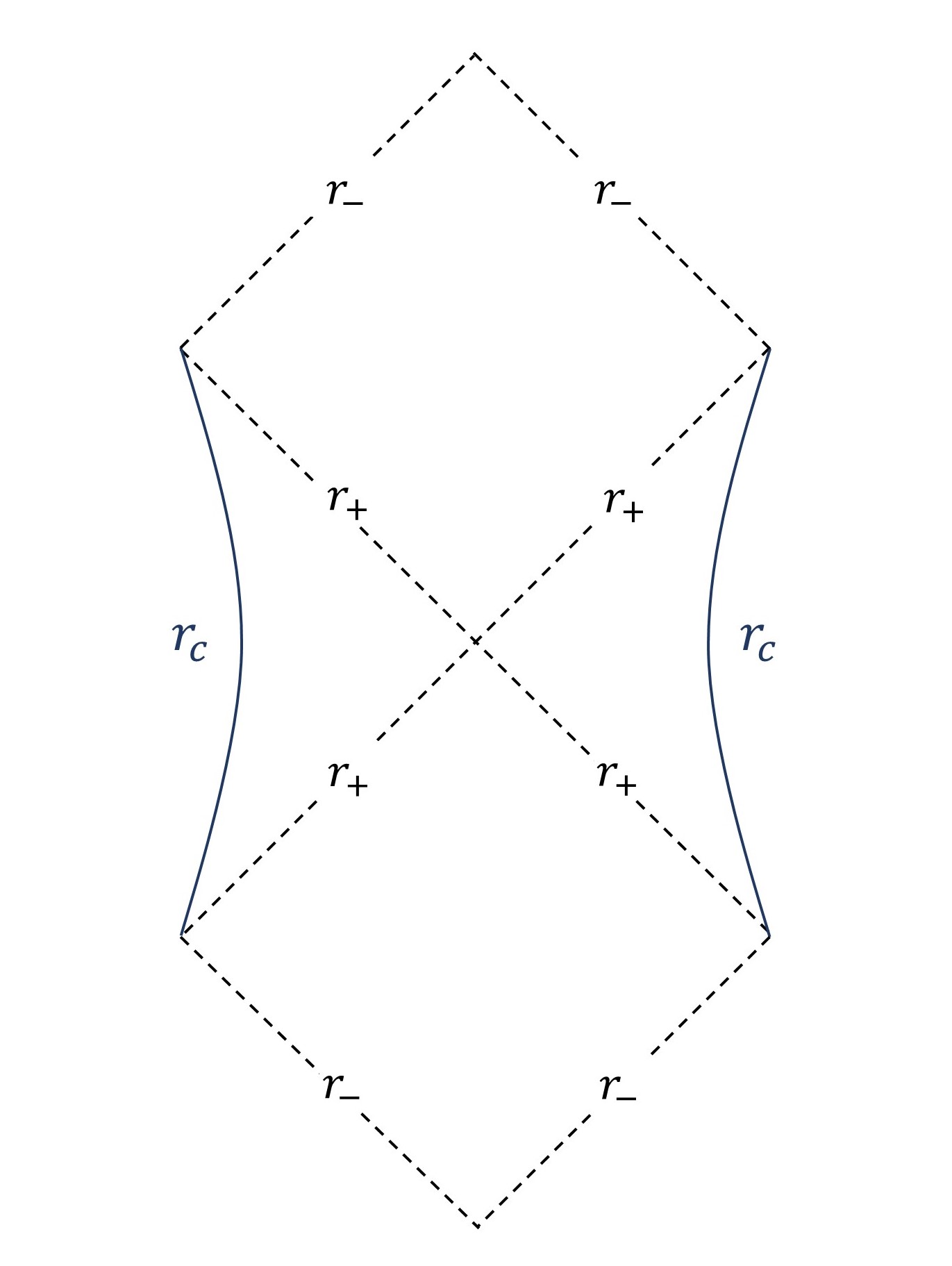
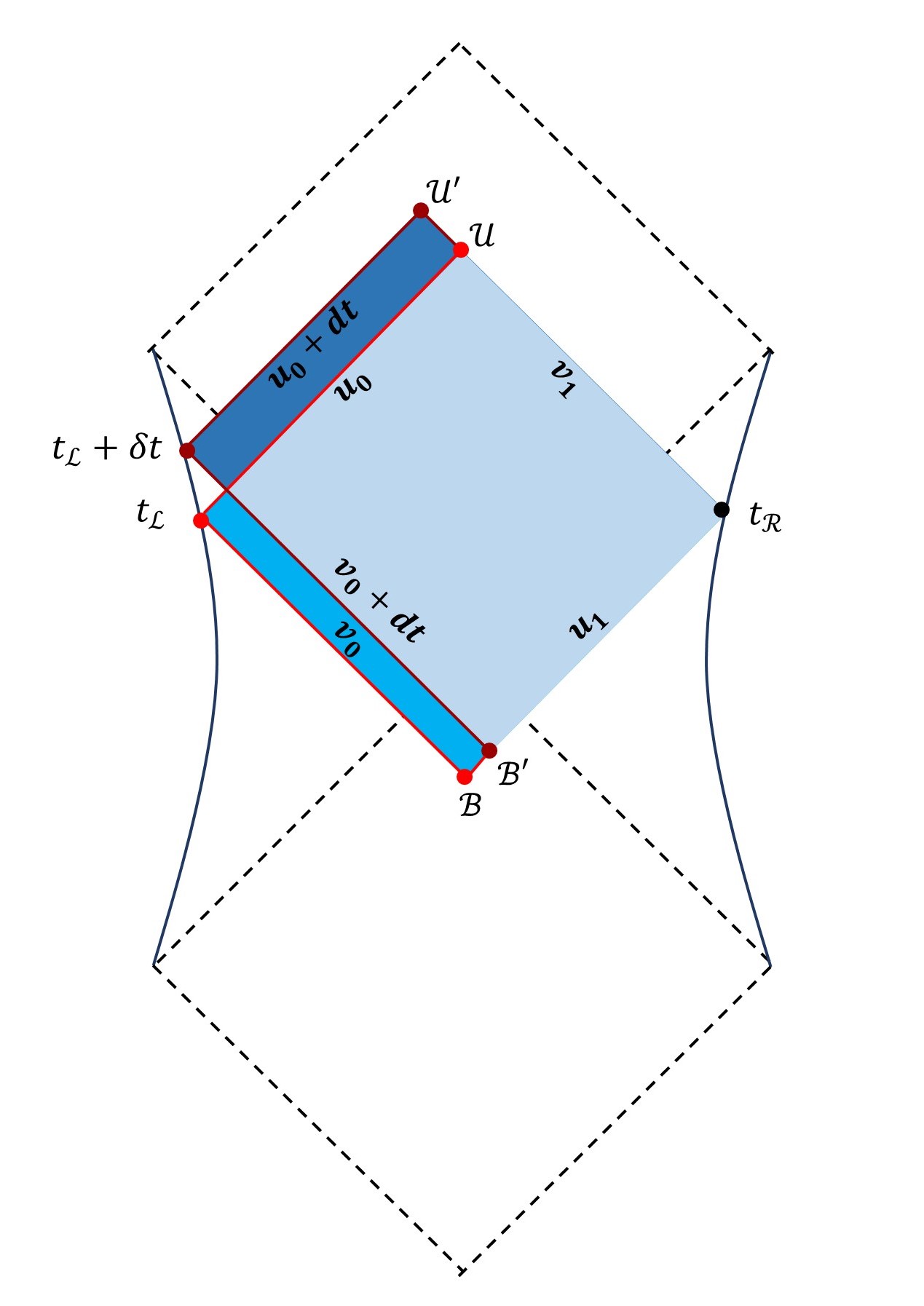
Figure 2: Left panel: The universal feature shared by the Penrose diagrams of $\text{AdS}_{2}$ black holes with multiple horizons (dashed lines), where $r_{\pm}$ are the outermost and next-to-outermost horizons, respectively, and $r_{c}$ corresponds to the UV-cutoff. Right panel: The change of WDW patches from the one anchored on $t_{L}$ and $t_{R}$ (pale blue and bright blue regions) to the one anchored on $t_{L}+\delta t$ and $t_{R}$ (pale blue and dark blue regions).

For neutral AdS black hole in 2D gravity with multiple horizons, the Penrose diagram shares the same feature as shown in Fig. 2. Now the total change of action due to the change of WDW patch reads

$$\delta\mathcal{A}_{\text{WDW}}=\delta\mathcal{A}^{\text{WDW}}_{\text{bulk}}+\delta\mathcal{A}^{\text{WDW}}_{\text{surf}}+\delta\mathcal{A}^{\text{WDW}}_{\text{joint}},$$ (27)

where the null surface terms can be made vanish with the choice of affine parameter for the generator of null surfaces, while the bulk and joint contributions are evaluated as

$$\delta\mathcal{A}^{\text{WDW}}_{\text{bulk}} =\frac{1}{2G}\int^{u_{0}+\delta t}_{u_{0}}\mathrm{d}u\int^{\rho(\frac{u-v_{0}-\delta t}{2})}_{\rho(\frac{u-v_{1}}{2})}\big{(}-\frac{\phi V^{\prime}(\phi)}{L^{2}}+\frac{V(\phi)}{L^{2}}\big{)}\mathrm{d}r$$

$$-\frac{1}{2G}\int_{v_{0}}^{v_{0}+\delta t}\mathrm{d}v\int_{\rho(\frac{u_{1}-v}{2})}^{\rho(\frac{u_{0}-v}{2})}\big{(}-\frac{\phi V^{\prime}(\phi)}{L^{2}}+\frac{V(\phi)}{L^{2}}\big{)}\mathrm{d}r$$

$$=\delta t\frac{\alpha j(\phi)}{G}\bigg{|}_{\phi_{\mathcal{U}}}^{\phi_{\mathcal{B}}}-\delta t\frac{\phi V(\phi)}{2G\alpha L^{2}}\bigg{|}_{\phi_{\mathcal{U}}}^{\phi_{\mathcal{B}}}~{}~{},$$ (28)

and

$$\delta\mathcal{A}^{\text{WDW}}_{\text{joint}} =\frac{1}{G}\big{(}\phi_{\mathcal{B}^{\prime}}a_{\mathcal{B}^{\prime}}-\phi_{\mathcal{B}}a_{\mathcal{B}}\big{)}+\frac{1}{G}\big{(}\phi_{\mathcal{U}^{\prime}}a_{\mathcal{U}^{\prime}}-\phi_{\mathcal{U}}a_{\mathcal{U}}\big{)}$$

$$=\frac{\delta t}{G}\Bigg{[}\frac{\alpha f(r)\log|\frac{f(r)}{c\bar{c}}|}{2}\bigg{|}_{r_{\mathcal{U}}}^{r_{\mathcal{B}}}+\frac{\phi V(\phi)}{2\alpha^{2}L^{2}}\bigg{|}^{\phi_{\mathcal{B}}}_{\phi_{\mathcal{U}}}\Bigg{]}~{},$$ (29)

respectively. Now the growth rate of total action at late-time for neutral $\mathrm{AdS}_{2}$ black holes with multiple horizons vanishes similarly as JT gravity Brown:2018bms ; Akhavan:2018wla ; Alishahiha:2018swh ; Goto:2018iay

$$\frac{\mathrm{d}\mathcal{A}_{\text{WDW}}}{\mathrm{d}t}\bigg{|}_{t\rightarrow+\infty}=\Big{(}\frac{\mathrm{d}\mathcal{A}^{\text{WDW}}_{\text{bulk}}}{\mathrm{d}t}+\frac{\mathrm{d}\mathcal{A}_{\text{joint}}^{\text{WDW}}}{\mathrm{d}t}\Big{)}\bigg{|}_{t\rightarrow+\infty}=\frac{\alpha j(\phi)}{G}\bigg{|}_{\phi_{-}}^{\phi_{+}}=0,$$ (30)

which will be remedied below in Sec.2.3 with similar methods as proposed in Brown:2018bms ; Akhavan:2018wla ; Alishahiha:2018swh as well as our new treatment from a dual charged black hole.

2.2 Charged black holes

We next move to the charged AdS black holes in 2D gravity with Einstein-Maxwell-dilaton action of form

$$\mathcal{A} =\frac{1}{2G}\int_{\mathcal{M}}\bigg{(}\phi R+\frac{V(\phi)}{L^{2}}-\frac{G}{2}W(\phi)F^{2}\bigg{)}\sqrt{-g}\mathrm{d}^{2}x+\frac{1}{G}\int_{\partial\mathcal{M}}\bigg{(}\phi K-\mathcal{L}_{\text{ct}}^{\text{cha}}(\phi)\bigg{)}\sqrt{-h}\mathrm{d}x~{},$$ (31)

where $\mathcal{L}_{\text{ct}}^{\text{cha}}$ is the counter term for charged black holes that renders the Euclidean on-shell action finite. With the ansatz of a linear dilaton and RN gauge

$$\phi(r,t)=\alpha r,~{}~{}\mathrm{d}s^{2}=-f(\phi)\mathrm{d}t^{2}+f(\phi)^{-1}\mathrm{d}r^{2},$$ (32)

the corresponding EOMs

$$R+\frac{1}{L^{2}}V^{\prime}(\phi)-\frac{G}{2}W^{\prime}(\phi)F^{2} =0~{},$$ (33)

$$\nabla_{\mu}\nabla_{\nu}\phi-g_{\mu\nu}\bigg{(}\nabla^{2}\phi-\frac{V(\phi)}{2L^{2}}\bigg{)}-\frac{GW(\phi)}{4}g_{\mu\nu}F^{2}+GW(\phi)F_{\mu\rho}F_{\nu}^{~{}\rho} =0~{},$$ (34)

$$\nabla_{\mu}\big{(}W(\phi)F^{\mu\nu}\big{)} =0~{},$$ (35)

could be solved as

$$A_{t} =\frac{Qk(\phi)}{\alpha},~{}~{}F_{tr}=-\frac{Q}{W(\phi)},~{}~{}F_{\mu\nu}F^{\mu\nu}=-\frac{2Q^{2}}{W(\phi)^{2}},$$ (36)

$$f(\phi) =-\frac{2GM}{\alpha}+j(\phi)-\frac{GQ^{2}}{\alpha^{2}}k(\phi),$$ (37)

$$j(\phi) =\int^{\phi}\frac{V(\phi^{\prime})}{\alpha^{2}L^{2}}\mathrm{d}\phi^{\prime},~{}~{}k(\phi)=\int^{\phi}\frac{1}{W(\phi^{\prime})}\mathrm{d}\phi^{\prime},$$ (38)

where $Q$ is the electric charge of the system. Similar to the neutral case, the potential is taken as $V(\phi)=2\phi+B+\sum\limits_{i}B_{i}\phi^{b_{i}}$ with $b_{i}\neq 0,1$. If one further specifies $W(\phi)=A\phi^{a}$, then the Ricci scalar

$$R=-\frac{2}{L^{2}}-\frac{1}{L^{2}}\sum_{i}b_{i}B_{i}\phi^{b_{i}-1}-\frac{aGQ^{2}}{A}\phi^{-1-a}$$ (39)

exhibits an asymptotically $\text{AdS}_{2}$ boundary provided that $0\neq b_{i}<1$ and $a\geq-1$. A curvature singularity arises at $\phi=0$ when $\exists$ $B_{i}\neq 0$ or $a>-1$.

2.2.1 Single horizon

The Penrose diagram for charged $\mathrm{AdS}_{2}$ black hole with a single horizon (non-extreme) is the same as the neutral case in Fig. 1, of which the change in WDW patch leads to similar change in action as

$$\delta\mathcal{A}_{\text{WDW}}=\delta\mathcal{A}^{\text{WDW}}_{\text{bulk}}+\delta\mathcal{A}_{\text{ren.}\text{surf}}^{\text{WDW}}+\delta\mathcal{A}^{\text{WDW}}_{\text{joint}},$$

like the case of neutral black hole, the surface term would be renormalized to obtain a reasonable result. The contribution from the bulk term is

$$\delta\mathcal{A}^{\text{WDW}}_{\text{bulk}} =\frac{1}{2G}\int^{u_{0}+\delta t}_{u_{0}}\mathrm{d}u\int^{\rho(\frac{u-v_{0}-\delta t}{2})}_{\rho(\frac{u-v_{1}}{2})}\big{(}\phi R+\frac{V(\phi)}{L^{2}}-\frac{G}{2}W(\phi)F^{2}\big{)}\mathrm{d}r$$

$$-\frac{1}{2G}\int_{v_{0}}^{v_{0}+\delta t}\mathrm{d}v\int_{\rho(\frac{u_{1}-v}{2})}^{\rho(\frac{u_{0}-v}{2})}\big{(}\phi R+\frac{V(\phi)}{L^{2}}-\frac{G}{2}W(\phi)F^{2}\big{)}\mathrm{d}r$$

$$=\delta t\bigg{(}\frac{\alpha j(\phi)}{G}-\frac{\phi V(\phi)}{2G\alpha L^{2}}+\frac{Q^{2}\phi}{2\alpha W(\phi)}\bigg{)}\bigg{|}^{\phi_{\mathcal{B}}}_{\phi_{c_{-}}},$$ (40)

the contribution from the renormalized-surface term is

$$\delta\mathcal{A}^{\text{WDW}}_{\text{ren.}\text{surf}} =-\frac{1}{G}\int_{u_{0}-r^{*}(r_{c_{-}})}^{u_{0}-r^{*}(r_{c_{-}})+\delta t}\sqrt{|h|}\mathrm{d}t\Big{(}\phi K-\frac{\alpha j(\phi)}{\sqrt{|f(\phi)|}}\Big{)}$$

$$=\delta t\bigg{(}\frac{-\phi V(\phi)}{2G\alpha L^{2}}+\frac{\phi Q^{2}}{2\alpha W(\phi)}+\frac{\alpha j(\phi)}{G}\bigg{)}\bigg{|}_{\phi=\phi_{c_{-}}},$$ (41)

and the contribution from the joint term is

$$\delta\mathcal{A}^{\text{WDW}}_{\text{joint}} =\frac{1}{G}(\phi_{\mathcal{B}^{\prime}}a_{\mathcal{B}^{\prime}}-\phi_{\mathcal{B}}a_{\mathcal{B}})$$

$$=\delta t\bigg{(}\frac{\phi V(\phi)}{2G\alpha L^{2}}-\frac{Q^{2}\phi}{2\alpha W(\phi)}+\frac{\alpha f(\phi_{\mathcal{B}})}{2G}\log\Big{|}\frac{f(\phi_{\mathcal{B}})}{c\bar{c}}\Big{|}\bigg{)}\bigg{|}_{\phi=\phi_{\mathcal{B}}}.$$ (42)

Hence the total variation of $\mathcal{A}_{\text{WDW}}$ is

$$\delta\mathcal{A}_{\text{WDW}} =\delta t\Big{(}\frac{\alpha j(\phi)}{G}+\frac{\alpha f(\phi)}{2G}\log\Big{|}\frac{f(\phi)}{c\bar{c}}\Big{|}\Big{)}\bigg{|}_{\phi=\phi_{\mathcal{B}}},$$ (43)

whose growth rate at late-time reads

$$\frac{\mathrm{d}\mathcal{A}_{\text{WDW}}}{\mathrm{d}t}\bigg{|}_{t\rightarrow+\infty} =2M-\mu Q,$$ (44)

where $\mu$ is the chemical potential of the charged black hole, see Appendix A.1.2 for more details. One can see that when $Q\rightarrow 0$, the action growth goes back to the neutral case as expected.

2.2.2 Multiple horizons

The Penrose diagram for charged $\mathrm{AdS}_{2}$ black hole with multiple horizons shares the same features as the neutral case in Fig. 2, of which the change in WDW patch leads to similar change in action as

$$\delta\mathcal{A}_{\text{WDW}}=\mathcal{A}^{\text{WDW}}_{\text{dark blue\&red}}-\mathcal{A}^{\text{WDW}}_{\text{bright blue\&red}}=\delta\mathcal{A}_{\text{bulk}}+\delta\mathcal{A}_{\text{joint}},$$

where the bulk contribution from Einstein-dilaton part is

$$\delta\mathcal{A}^{\text{WDW}}_{\text{bulk}_{1}} =\frac{1}{2G}\int_{\delta v}\bigg{(}\phi R+\frac{V}{L^{2}}\bigg{)}\sqrt{-g}\mathrm{d}^{2}x$$

$$=\delta t\bigg{(}\frac{\alpha j(\phi)}{G}-\frac{\phi V(\phi)}{2G\alpha L^{2}}-\frac{Q^{2}k(\phi)}{2\alpha}+\frac{Q^{2}\phi}{2\alpha W(\phi)}\bigg{)}\Bigg{|}^{\phi_{\mathcal{B}}}_{\phi_{\mathcal{U}}},$$ (45)

and the bulk contribution from Einstein-Maxwell part is

$$\delta\mathcal{A}^{\text{WDW}}_{\text{bulk}_{2}} =-\frac{1}{4}\int_{\delta v}W(\phi)F^{2}\sqrt{-g}\mathrm{d}^{2}x$$

$$=\delta t\frac{Q^{2}k(\phi)}{2\alpha}\bigg{|}^{\phi_{\mathcal{B}}}_{\phi_{\mathcal{U}}}.$$ (46)

The contribution from the joint term is

$$\delta\mathcal{A}^{\text{WDW}}_{\text{joint}} =\frac{1}{G}\big{(}\phi_{\mathcal{B}^{\prime}}a_{\mathcal{B}^{\prime}}-\phi_{\mathcal{B}}a_{\mathcal{B}}\big{)}+\frac{1}{G}\big{(}\phi_{\mathcal{U}^{\prime}}a_{\mathcal{U}^{\prime}}-\phi_{\mathcal{U}}a_{\mathcal{U}}\big{)}$$

$$=\delta t\bigg{(}\frac{\phi V(\phi)}{2G\alpha L^{2}}-\frac{Q^{2}\phi}{2\alpha W(\phi)}\bigg{)}\bigg{|}^{\phi_{\mathcal{B}}}_{\phi_{\mathcal{U}}}+\delta t\frac{f(r)\log\frac{-f(r)}{c\bar{c}}}{2G}\bigg{|}_{r_{\mathcal{U}}}^{r_{\mathcal{B}}}.$$ (47)

Hence the total variation is

$$\delta\mathcal{A}_{\text{WDW}} =\delta\mathcal{A}^{\text{WDW}}_{\text{bulk}_{1}}+\delta\mathcal{A}^{\text{WDW}}_{\text{bulk}_{2}}+\delta\mathcal{A}^{\text{WDW}}_{\text{joint}}$$

$$=\delta t\frac{\alpha j(\phi)}{G}\bigg{|}^{\phi_{\mathcal{B}}}_{\phi_{\mathcal{U}}}+\delta t\frac{f(r)\log\frac{-f(r)}{c\bar{c}}}{2G}\bigg{|}_{r_{\mathcal{U}}}^{r_{\mathcal{B}}},$$ (48)

whose growth rate at late-time reads

$$\frac{\mathrm{d}\mathcal{A}_{\text{WDW}}}{\mathrm{d}t}\bigg{|}_{t\rightarrow+\infty}=\frac{\alpha j(\phi)}{G}\bigg{|}_{\phi_{-}}^{\phi_{+}}=\mu_{-}Q-\mu_{+}Q~{}.$$ (49)

2.3 Resolutions for vanishing late-time growth rate

To resolve the vanishing growth rate of action at late-time for neutral $\mathrm{AdS}_{2}$ black holes with multiple horizons, a JT-like gravity of form

$$\mathcal{A}_{\text{JT-like}} =\frac{\phi_{0}}{2G}\int_{\mathcal{M}}\mathrm{d}^{2}x\sqrt{-g}R+\frac{\phi_{0}}{G}\int_{\partial\mathcal{M}}\mathrm{d}x\sqrt{-h}K$$

$$+\frac{1}{2G}\int_{\mathcal{M}}\mathrm{d}^{2}x\sqrt{-g}\Big{(}\phi R+\frac{2\phi-3\frac{\phi^{2}}{\phi_{0}}}{L^{2}}\Big{)}+\frac{1}{G}\int_{\partial\mathcal{M}}\mathrm{d}x\sqrt{-h}\big{(}\phi K-\frac{\sqrt{\phi^{2}-\frac{\phi^{3}}{\phi_{0}}}}{L}\big{)}$$ (50)

is adopted for illustration, where $\phi/\phi_{0}\ll 1$ for a positive $\phi_{0}$. For a specific solution of form

$$\phi =\frac{r}{L},$$ (51)

$$\mathrm{d}s^{2} =-f(\phi)\mathrm{d}t^{2}+f(\phi)^{-1}\mathrm{d}r^{2},$$ (52)

$$f(\phi) =-2GML+\phi^{2}-\frac{\phi^{3}}{\phi_{0}}$$ (53)

$$=-2+\phi^{2}-\frac{\phi^{3}}{100},$$ (54)

with $\phi_{0}=100,~{}GML=1$, $f(\phi)$ exhibits three real roots

$$\phi_{1} \approx 99.9800~{},$$ (55)

$$\phi_{+} \approx 1.4244~{},$$ (56)

$$\phi_{-} \approx-1.4044~{}.$$ (57)

Since $\phi_{1}/\phi_{0}\approx 1$ and here we have assumed $\phi/\phi_{0}\ll 1$ , $\phi_{1}$ could be neglected. The black hole could be regarded as having double horizons, whose Penrose diagram is shown in Fig.3 and contains the feature shown in Fig. 2. Hence the action growth rate at late-time is also vanishing. To restore the linear growth of holographic complexity, we first follow the two approaches proposed in Brown:2018bms ; Alishahiha:2018swh .

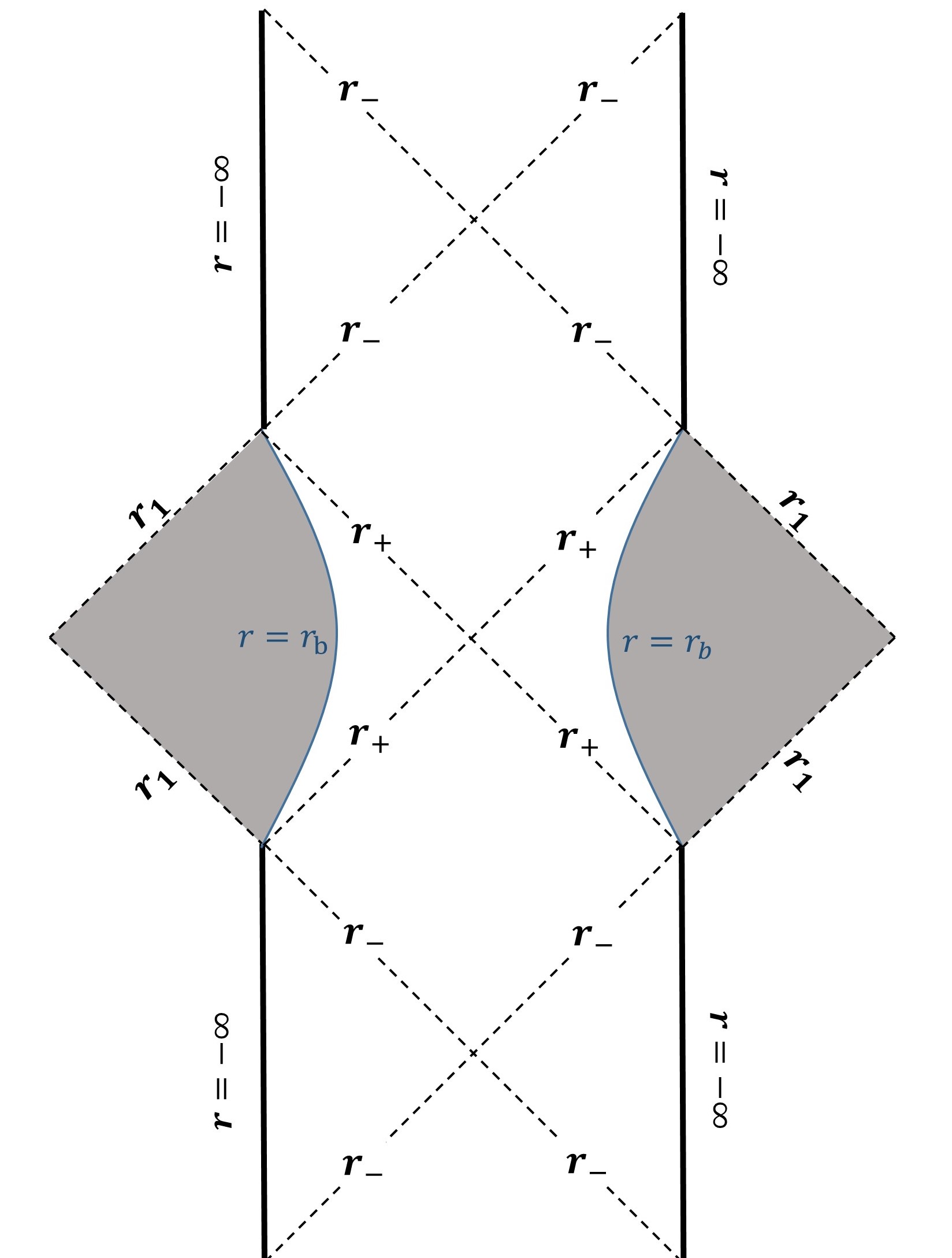
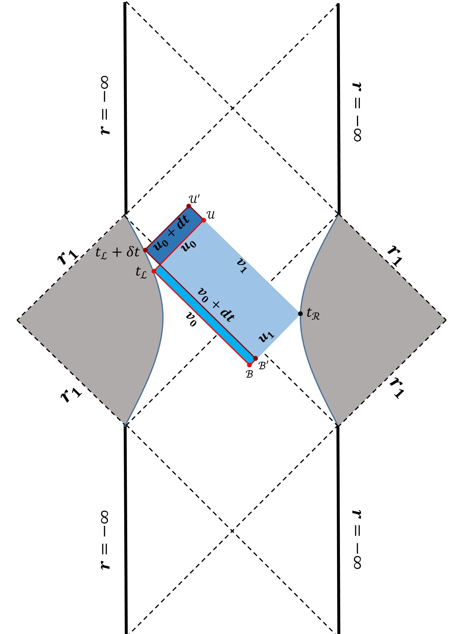
Figure 3: Left panel: Penrose diagram for the JT-like black hole (50) with outer and inner horizons at $r=r_{\pm}$ (dashed lines), UV cutoff boundaries at $r=r_{b}$ (blue lines), and conformal boundaries at $r=\pm\infty$. Right panel: The change of WDW patches from the one anchored on $t_{L}$ and $t_{R}$ (pale blue and bright blue regions) to the one anchored on $t_{L}+\delta t$ and $t_{R}$ (pale blue and dark blue regions).

2.3.1 Electromagnetic boundary term

The JT-like gravity could also be obtained from dimensional reduction of four-dimensional (4D) RN black hole with action of form

$$\widetilde{\mathcal{A}}_{\text{RN}} =\frac{1}{16\pi}\int_{\mathcal{M}}\mathrm{d}^{4}x\sqrt{-g}\bigg{(}\frac{1}{\ell^{2}}R-F_{\mu\nu}F^{\mu\nu}\bigg{)}+\frac{1}{8\pi}\int_{\partial\mathcal{M}}\mathrm{d}^{3}x\sqrt{-h}\frac{1}{\ell^{2}}\bigg{(}K-K_{0}\bigg{)}$$

$$+\frac{1}{4\pi}\int_{\partial\mathcal{M}}\mathrm{d}^{3}x\sqrt{-h}n_{\mu}F^{\mu\nu}A_{\nu},$$ (58)

where $\ell^{2}$ is the 4D Newton constant $G_{N}$. After adopting an ansatz for a spherically symmetric metric

$$\mathrm{d}s^{2}=\frac{1}{\sqrt{2\Phi}}g_{ij}\mathrm{d}x^{i}\mathrm{d}x^{j}+2\ell^{2}\Phi\mathrm{d}\Omega^{2},$$ (59)

the first line in the action (58) becomes

$$\widetilde{\mathcal{A}}_{2d}=\frac{1}{2}\int\mathrm{d}^{2}x\sqrt{-g}\bigg{(}\Phi R+\frac{1}{\ell^{2}}(2\Phi)^{-\frac{1}{2}}+\frac{\ell^{2}}{2}(2\Phi)^{\frac{3}{2}}F_{ij}F^{ij}\bigg{)}+\int\mathrm{d}x\sqrt{-h}\bigg{(}\Phi K-\frac{1}{\ell}\big{(}2\Phi\big{)}^{\frac{1}{4}}\bigg{)}.$$ (60)

After further evaluated at an on-shell electromagnetic field strength, the resulting 2D action reads

$$\widetilde{\mathcal{A}}^{2d}_{\text{on-shell}} =\frac{1}{2}\int_{\mathcal{M}}\mathrm{d}^{2}x\sqrt{-g}\Big{(}\Phi R+\frac{1}{\ell^{2}}(2\Phi)^{-\frac{1}{2}}-\frac{Q^{2}}{\ell^{2}}(2\Phi)^{-\frac{3}{2}}\Big{)}+\int_{\partial\mathcal{M}}\mathrm{d}x\sqrt{-h}\bigg{(}\Phi K-\frac{1}{\ell}\big{(}2\Phi\big{)}^{\frac{1}{4}}\bigg{)},$$ (61)

where the rescaled bulk term $\mathcal{A}\equiv\tilde{\mathcal{A}}/G$ could be rewritten as

$$\mathcal{A}_{\text{bulk}} =\frac{\phi_{0}}{2G}\int\mathrm{d}^{2}x\sqrt{-g}R+\frac{1}{2G}\int\mathrm{d}^{2}x\sqrt{-g}\Big{(}\phi R+\frac{1}{L^{2}}V(\phi)\Big{)}$$ (62)

$$=\frac{\phi_{0}}{2G}\int\mathrm{d}^{2}x\sqrt{-g}R+\frac{\phi_{0}}{2G}\int\mathrm{d}^{2}x\sqrt{-g}\bigg{(}\frac{\phi}{\phi_{0}}R+\frac{1}{L^{2}}\sum_{n=1}^{N}\frac{(-1)^{n+1}\prod_{k=1}^{n}(2k-1)}{2^{n-2}(n-1)!}\frac{\phi^{n}}{\phi_{0}^{n}}\bigg{)}$$ (63)

by expanding $\Phi$ around $\phi_{0}=Q^{2}/2$ upto to $N$-th order and abbreviating $L\equiv Q^{\frac{3}{2}}\ell$. For $N=2$, the resulting bulk action

$$\mathcal{A}_{\text{bulk}} =\frac{\phi_{0}}{2G}\int_{\mathcal{M}}\mathrm{d}^{2}x\sqrt{-g}R+\frac{\phi_{0}}{2G}\int_{\mathcal{M}}\mathrm{d}^{2}x\sqrt{-g}\Big{(}\frac{\phi}{\phi_{0}}R+\frac{2\frac{\phi}{\phi_{0}}-3\frac{\phi^{2}}{\phi_{0}^{2}}}{L^{2}}\Big{)}$$ (64)

coincides with the Eq.(50) as expected from dimensional reduction of 4D RN black hole.

The second line in the action (58) is a 4D electromagnetic boundary term suggested in Brown:2018bms , which induces a 2D boundary electromagnetic boundary term

$$\mathcal{A}^{2d}_{\text{em.bdy}} =\frac{\ell^{2}}{G}\int_{\partial\mathcal{M}}\mathrm{d}x\sqrt{-h}(2\Phi)^{\frac{3}{2}}n_{i}F^{ij}A_{j}$$

$$=-\frac{Q^{2}}{G\ell^{2}}\int_{\mathcal{M}}\mathrm{d}^{2}x\sqrt{-g}(2\Phi)^{-\frac{3}{2}}.$$ (65)

This should also contribute to the would-be restored JT-like action by $\mathcal{A}_{\text{JT-like}}^{\text{restored}}=\mathcal{A}^{\text{WDW}}_{\text{JT-like}}-\mathcal{A}^{\text{WDW}}_{\text{em.bdy}}$ when evaluated on the WDW patch. Since the first term $\mathcal{A}^{\text{WDW}}_{\text{JT-like}}$ has vanishing growth rate according to Eq.(30), then the growth rate of the restored action at late-time simply reads

$$\frac{\mathrm{d}\mathcal{A}_{\text{JT-like}}^{\text{restored}}}{\mathrm{d}t}\bigg{|}_{t\rightarrow+\infty}=-\frac{\mathrm{d}\mathcal{A}^{\text{WDW}}_{\text{em.bdy}}}{\mathrm{d}t}\bigg{|}_{t\rightarrow+\infty}.$$ (66)

After expanded in terms of $\phi\sim\phi_{0}$ up to the second order, the contribution from the electromagnetic boundary term reads

$$\frac{\mathrm{d}\mathcal{A}^{\text{WDW}}_{\text{em.bdy}}}{\mathrm{d}t}\bigg{|}_{t\rightarrow+\infty} =-4\frac{\phi_{0}\phi_{+}}{GL}+2\frac{\phi_{+}^{2}}{GL}-\frac{3}{2}\frac{\phi_{+}^{3}}{\phi_{0}GL}+\mathcal{O}(\frac{\phi_{+}^{2}}{\phi_{0}^{2}}\phi_{+}^{2}).$$ (67)

Therefore, the restored growth rate of $\mathcal{A}_{\text{WDW}}$ at late-time is

$$\frac{\mathrm{d}\mathcal{A}_{\text{JT-like}}^{\text{restored}}}{\mathrm{d}t}\bigg{|}_{t\rightarrow+\infty}=4\frac{\phi_{0}\phi_{+}}{GL}-2\frac{\phi_{+}^{2}}{GL}+\frac{3}{2}\frac{\phi_{+}^{3}}{\phi_{0}GL}+\mathcal{O}(\frac{\phi_{+}^{2}}{\phi_{0}^{2}}\phi_{+}^{2}),$$ (68)

which could be expressed in terms of the thermodynamic quantities

$$T =\frac{\phi_{+}}{2\pi L}-\frac{3\phi_{+}^{2}}{4\pi L\phi_{0}},~{}~{}S=\frac{2\pi(\phi_{0}+\phi_{+})}{G},~{}~{}M=\frac{\phi_{+}^{2}}{2GL}-\frac{\phi_{+}^{3}}{2GL\phi_{0}}$$ (69)

as

$$\frac{\mathrm{d}\mathcal{A}_{\text{JT-like}}^{\text{restored}}}{\mathrm{d}t}\bigg{|}_{t\rightarrow+\infty}=4ST+G(10M+5S_{0}T-5ST)=4ST+\mathcal{O}\big{(}\frac{\phi_{+}}{\phi_{0}}\phi_{+}^{2}\big{)}$$ (70)

with $S_{0}\equiv\frac{2\pi\phi_{0}}{G}$. The growth rate (70) of the JT-like gravity is identical to the growth rate of the JT gravity given in Brown:2018bms on the leading-order. Since the JT-like gravity we demonstrated can be reduced to JT gravity by discarding the sub-leading potential with respect to $\phi\over\phi_{0}$,i.e., $\frac{\phi^{2}}{\phi_{0}^{2}}$, see (64), the consistency of late-time growth rate indicate that the higher-order correction of dilaton potential in (50) does not affect the leading order of late-time growth rate but only the sub-leading order.

2.3.2 UV/IR relation for cutoff surfaces

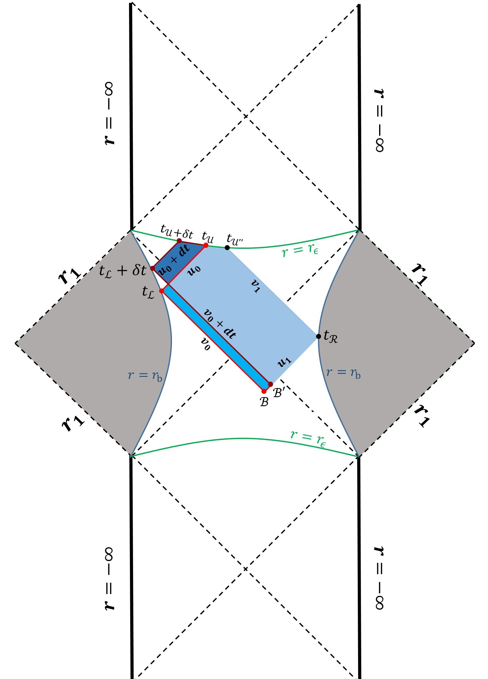
Figure 4: Penrose diagram for JT-like gravity with both UV cutoff surface $r=r_{b}$ (blue line) at asymptotic boundary and IR cutoff surface $r=r_{\epsilon}$(green line) behind the outer horizon.

To recover the linear action growth rate at late-time in JT gravity, Akhavan:2018wla proposed an alternative prescription by relating the IR cutoff surface $r=r_{\epsilon}$ behind the horizon with the UV cutoff surface $r=r_{b}$ at asymptotic boundary upto the leading-order

$$r_{\epsilon}=\frac{r_{+}^{3}}{r_{b}^{2}},$$ (71)

and an appropriate counter term Alishahiha:2018swh should also be appreciated on the cutoff surface behind the horizon as shown with green line in Fig. 4. However, there is generally no universal determination for the extra counter term on the $r=r_{\epsilon}$. Here we introduce an counter term of form $\mathcal{L}^{\mathrm{ct}}_{\text{JT-like}}[\phi_{0}]=\frac{\sqrt{2}\phi_{0}}{L}$ for the JT-like gravity (50), so that the total action

$$\mathcal{A}_{\text{JT-like}}^{\text{cut-off}} =\mathcal{A}_{\text{JT-like}}-\frac{\phi_{0}}{G}\int_{\text{bdy},r=r_{\epsilon}}\mathrm{d}x\sqrt{-h}\frac{\sqrt{2}}{L}$$ (72)

exhibits a growth rate

$$\frac{\mathrm{d}\mathcal{A}^{\text{cut-off}}_{\text{JT-like}}}{\mathrm{d}t}\bigg{|}_{t\rightarrow+\infty} =\frac{\sqrt{2}\phi_{0}\phi_{+}}{GL}+\frac{\sqrt{2}\phi_{+}^{2}}{2GL}+\frac{4-3\sqrt{2}}{4}\frac{\phi_{+}^{3}}{\phi_{0}GL}+\mathcal{O}\big{(}\frac{\phi_{+}^{2}}{\phi_{0}^{2}}\phi_{+}^{2}\big{)}$$ (73)

that could be rewritten in terms of thermodynamic quantities as

$$\frac{\mathrm{d}\mathcal{A}_{\text{restored}}}{\mathrm{d}t}\bigg{|}_{t\rightarrow+\infty}=\sqrt{2}ST+\mathcal{O}\big{(}\phi_{+}^{2}\big{)}.$$ (74)

Compared with the growth rate of JT gravity in Alishahiha:2018swh

$$\frac{\mathrm{d}\mathcal{A}^{\text{WDW}}_{\text{JT}}}{\mathrm{d}t}\bigg{|}_{t\rightarrow+\infty}=ST+\mathcal{O}(\phi_{+}^{2}),$$ (75)

the different coefficients in front of $ST$ come from the different counter term $\mathcal{L}_{\mathrm{ct}}(\phi_{0})$ used.

2.3.3 Charged dual of neutral black hole

Apart from the previous two resolutions, we propose here a third solution by relating the neutral and charged $\mathrm{AdS}_{2}$ black holes. Recall that the charged black hole has an action of form

$$\mathcal{A}_{\text{cha}}=\frac{1}{2G}\int\mathrm{d}^{2}x\sqrt{|g|}\Big{(}\phi R+\frac{V(\phi)}{L^{2}}\Big{)}-\frac{1}{4}\int\mathrm{d}^{2}x\sqrt{|g|}W(\phi)F_{\mu\nu}F^{\mu\nu}+\text{GHY term},$$ (76)

of which the EOMs and corresponding solution are showed in Eq.(33—35) and Eq.(36—38) respectively. As pointed out in Grumiller:2007ju , the metric (37) could also be obtained from an uncharged black hole by replacing $V(\phi)$ in (9) with an effective potential of the form

$$V^{\text{eff}}(\phi)\equiv V(\phi)-\frac{GQ^{2}L^{2}}{W(\phi)},$$ (77)

and the charged and uncharged black hole have the same temperature and Wald entropy. In this sense, there is a dual relation between charged black holes and neutral black holes. Given a charged black hole with dilaton potential $V(\phi)$, coupling function $W(\phi)$ and electric charge $Q$, the bulk on-shell action is

$$\mathcal{A}^{\text{cha}}_{\text{bulk}} =\frac{1}{2G}\int\mathrm{d}^{2}x\sqrt{|g|}\Big{(}\phi R+\frac{V(\phi)}{L^{2}}\Big{)}-\frac{1}{4}\int\mathrm{d}^{2}x\sqrt{|g|}W(\phi)F^{2}$$

$$=\frac{1}{2G}\int\mathrm{d}^{2}x\sqrt{|g|}\bigg{(}-\frac{\phi V^{\prime}(\phi)}{L^{2}}+\frac{V(\phi)}{L^{2}}-\frac{GQ^{2}\phi W^{\prime}(\phi)}{W(\phi)^{2}}+\frac{GQ^{2}}{W(\phi)}\bigg{)},$$ (78)

while the on-shell bulk action of dual neutral black hole with effective potential (77) is

$$\mathcal{A}^{\text{neu}}_{\text{bulk}} =\frac{1}{2G}\int\mathrm{d}^{2}x\sqrt{|g|}\bigg{(}\phi R+\frac{V^{\text{eff}}(\phi)}{L^{2}}\bigg{)}$$

$$=\frac{1}{2G}\int\mathrm{d}^{2}x\sqrt{|g|}\bigg{(}-\frac{\phi V^{\prime}(\phi)}{L^{2}}+\frac{V(\phi)}{L^{2}}-\frac{GQ^{2}\phi W^{\prime}(\phi)}{W(\phi)^{2}}-\frac{GQ^{2}}{W(\phi)}\bigg{)},$$ (79)

with flipped sign for $\frac{GQ^{2}}{W(\phi)}$. The difference between (79) and (78) can be rewritten as an additional electric boundary term by using the on-shell electromagnetic field strength (36)

$$-\int\frac{Q^{2}}{W(\phi)}d\phi=\frac{1}{2}\int dx\sqrt{-h}n_{\mu}W(\phi)F^{\mu\nu}A_{\nu}.$$ (80)

For the neutral black hole with the effective potential (77), the action of the corresponding charged black hole is Eq.(76) plus Eq.(80). In this sense, the neutral black hole with multiple horizons corresponds to the charged one with varying chemical potential in an ensemble with charged fixed.

To see how the linear growth rate at late-time is restored for neutral $\mathrm{AdS}_{2}$ black hole with multiple horizons, we start with following action

$$\mathcal{A}=\frac{1}{2G}\int\mathrm{d}^{2}x\sqrt{|g|}\bigg{(}\Phi R+\frac{(2\Phi)^{-\frac{1}{2}}-G^{2}\lambda^{2}(2\Phi)^{-\frac{3}{2}}}{\ell^{2}}\bigg{)}+\text{GHY term},$$ (81)

where the JT gravity could be induced from keeping the first order expansion of the dilaton around $\Phi=\phi_{0}=\frac{(G\lambda)^{2}}{2}$, namely,

$$\mathcal{A}\approx\frac{\phi_{0}}{2G}\int\mathrm{d}^{2}x\sqrt{-g}R+\frac{1}{2G}\int\mathrm{d}^{2}x\sqrt{-g}\phi\Big{(}R+\frac{2}{L^{2}}\Big{)}+\text{High order terms}~{},$$ (82)

with $L^{2}=(G\lambda)^{3}\ell^{2}$. The dual charged black hole of (81) could be identified by defining

$$V(\Phi)=(2\Phi)^{-\frac{1}{2}},~{}~{}W(\Phi)=\frac{\ell^{2}}{G}(2\Phi)^{\frac{3}{2}},~{}~{}Q=\lambda~{},$$ (83)

and the corresponding action reads

$$\mathcal{A}_{\text{dual}} =\frac{1}{2G}\int\mathrm{d}^{2}x\sqrt{|g|}\Big{(}\Phi R+\frac{1}{\ell^{2}}(2\Phi)^{-\frac{1}{2}}\Big{)}-\frac{1}{4}\int\mathrm{d}^{2}x\sqrt{|g|}\frac{\ell^{2}}{G}(2\Phi)^{\frac{3}{2}}F^{\mu\nu}F_{\mu\nu}+\text{GHY term}$$

$$+\frac{1}{2}\int dx\sqrt{-h}\frac{\ell^{2}}{G}(2\Phi)^{\frac{3}{2}}n_{\mu}F^{\mu\nu}A_{\nu}.$$ (84)

According to Eq.(49), the late-time action growth rate of the dual charged black hole (84) without the electric boundary term (80) is

$$\frac{\mathrm{d}\mathcal{A}_{\text{dual}}}{\mathrm{d}t}\bigg{|}_{t\rightarrow+\infty} =\mu_{-}\lambda-\mu_{+}\lambda,~{}~{}~{}~{}\mu_{\pm}=-\frac{\lambda k(\Phi_{\pm})}{\alpha}.$$ (85)

After expanding $\Phi_{\pm}$ in (85) around $\phi_{0}$, $\Phi_{\pm}=\phi_{0}\pm\phi_{+}$, one can obtain the restored growth rate for JT gravity

$$\frac{\mathrm{d}\mathcal{A}^{\text{restored}}_{\text{JT}}}{\mathrm{d}t}\bigg{|}_{t\rightarrow+\infty}=\frac{2G\lambda^{2}}{\alpha L^{2}}\phi_{+}~{}+\mathcal{O}\big{(}\phi_{+}^{2}\big{)}=4ST+\mathcal{O}(T^{2}).$$ (86)

This is the same as found in Brown:2018bms .

3 CV 1.0

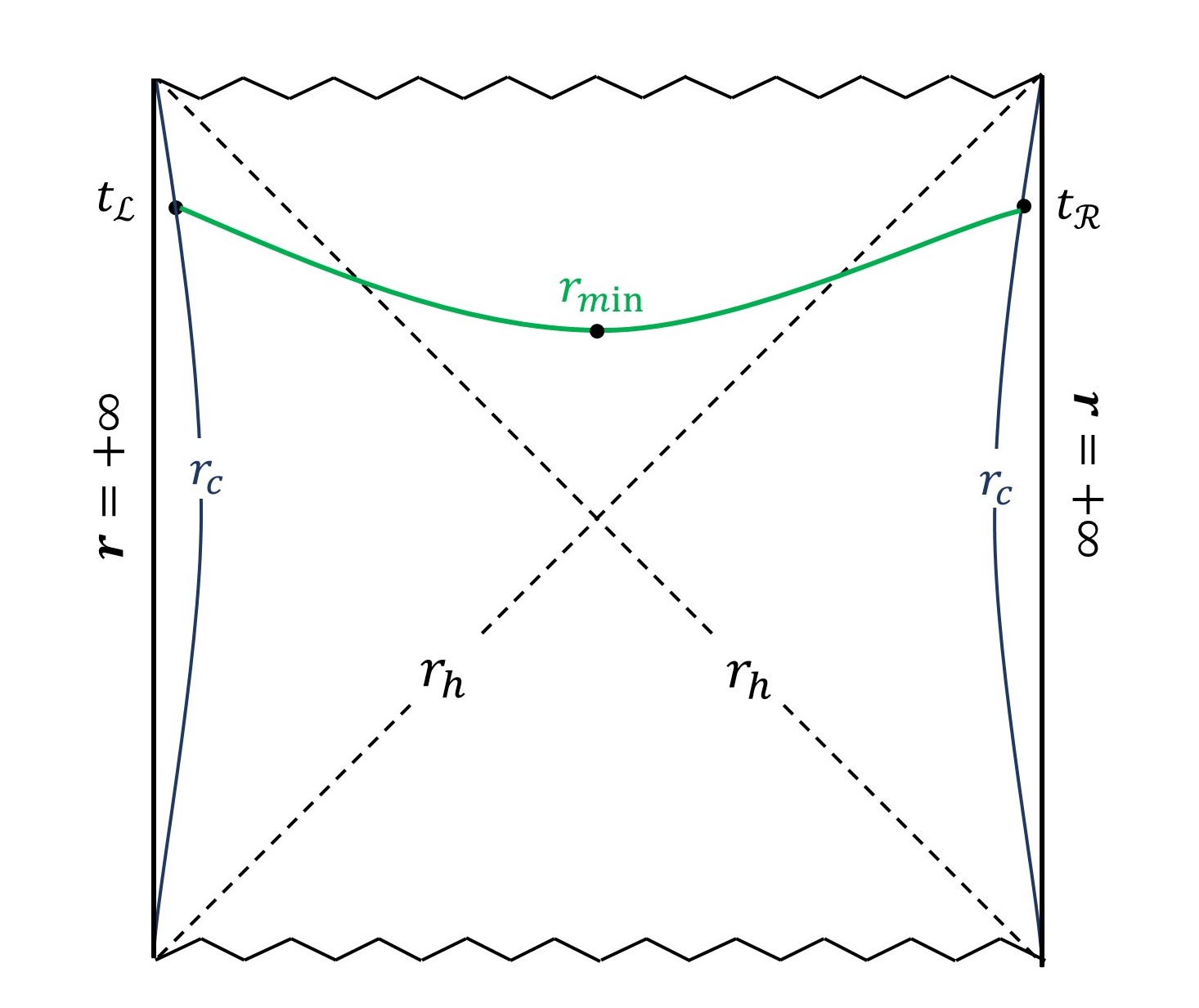
Figure 5: The extremal surface (green line) anchored at $t_{\mathrm{L}}$ and $t_{\mathrm{R}}$ on the boundaries regulated by the UV cutoff surfaces at $r_{c}$.

In this section, we investigate in the context of 2D gravity the CV 1.0 conjecture Susskind:2014rva ; Stanford:2014jda , which claims a proportionality between the complexity of the TFD state living on the boundaries and the volume of extremal/maximal time slice anchored at the boundary times $t_{L}$ and $t_{R}$ as shown in Fig. 5, namely,

$$\mathcal{C}_{\mathcal{V}}=\max\left[\frac{\mathcal{V}}{G\ell}\right],$$ (87)

where the characteristic scale $\ell$ is set by the $\mathrm{AdS}_{2}$ radius $L$ for simplicity. Due to the symmetry of TFD state under boundary time shift $t_{L}\to t_{L}+\Delta t$, $t_{R}\to t_{R}-\Delta t$, the volume should only depend on the total boundary time $t=t_{L}+t_{R}$, where a symmetric setup $t_{L}=t_{R}$ could be adopted for convenience. Note that the extremal volume behind the horizon exhibits an upper bound Yang:2019alh . Following the technique from Carmi:2017jqz , we can similarly compute the growth rate of extremal volume for 2D gravity as shown below.

3.1 Growth rate of extremal volume

Armed with the in-falling Eddington-Finkelstein coordinate $v=t+r^{*}(r)$, the metric becomes $\mathrm{d}s^{2}=-f(r)\mathrm{d}v^{2}+2\mathrm{d}v\mathrm{d}r$, and hence the volume of the extremal surface parameterized by $r(\lambda)$ and $v(\lambda)$ could be computed by

$$\mathcal{V}=\int\mathrm{d}\lambda\mathcal{L}(r,\dot{r},\dot{v}),\quad\mathcal{L}(r,\dot{r},\dot{v})\equiv\sqrt{-f(r)\dot{v}^{2}+2\dot{v}\dot{r}},$$ (88)

where the independence of $\mathcal{L}$ on $v$ gives rise to a conserved quantity $E$ defined by

$$E=-\frac{\partial\mathcal{L}}{\partial\dot{v}}=\frac{f\dot{v}-\dot{r}}{\sqrt{-f\dot{v}^{2}+2\dot{v}\dot{r}}}.$$ (89)

On the other hand, the reparametrization invariance of volume with respect to the choice of $\lambda$ implies that $-f\dot{v}^{2}+2\dot{v}\dot{r}=1$, therefore, the extremal surface could be determined by

$$E =f(r)\dot{v}-\dot{r},$$ (90)

$$\dot{r}^{2} =f(r)+E^{2},$$ (91)

and the maximal volume becomes

$$\mathcal{V}=2\int_{r_{\mathrm{min}}}^{r_{\mathrm{max}}}\frac{\mathrm{d}r}{\dot{r}}=2\int_{r_{\mathrm{min}}}^{r_{\mathrm{max}}}\frac{\mathrm{d}r}{\sqrt{f(r)+E^{2}}},$$ (92)

where $r_{\mathrm{min}}$ is determined by the condition $\dot{r}=0$, namely, $f(r_{\mathrm{min}})+E^{2}=0$. To further evaluate the maximal volume, there is a trick by first noting that

$$t_{R}+r^{*}(\infty)-r^{*}(r_{\mathrm{min}}) =\int_{v_{\mathrm{min}}}^{v_{\infty}}\mathrm{d}v=\int_{r_{\mathrm{min}}}^{\infty}\mathrm{d}r\frac{\dot{v}}{\dot{r}}=\int_{r_{\mathrm{min}}}^{\infty}\mathrm{d}r\left[\frac{f(r)\dot{v}-\dot{r}}{f(r)\dot{r}}+\frac{1}{f(r)}\right]$$ (93)

$$=\int_{r_{\mathrm{min}}}^{\infty}\mathrm{d}r\left[\frac{E}{f(r)\sqrt{f(r)+E^{2}}}+\frac{1}{f(r)}\right],$$ (94)

then it is easy to see that

$$\frac{\mathcal{V}}{2}+E(t_{R}+r^{*}_{\infty}-r^{*}_{\mathrm{min}}) =\int_{r_{\mathrm{min}}}^{\infty}\mathrm{d}r\left[\frac{1}{\sqrt{f(r)+E^{2}}}+\frac{E}{f(r)\sqrt{f(r)+E^{2}}}+\frac{1}{f(r)}\right]$$ (95)

$$=\int_{r_{\mathrm{min}}}^{\infty}\mathrm{d}r\left[\frac{\sqrt{f(r)+E^{2}}}{f(r)}+\frac{E}{f(r)}\right],$$ (96)

which, after taken time derivative with respect to $t_{R}$, gives rise to

$$\frac{1}{2}\frac{\mathrm{d}\mathcal{V}}{\mathrm{d}t_{R}}+\frac{\mathrm{d}E}{\mathrm{d}t_{R}}(t_{R}+r^{*}_{\infty}-r^{*}_{\mathrm{min}})+E =\int_{r_{\mathrm{min}}}^{\infty}\mathrm{d}r\frac{\mathrm{d}E}{\mathrm{d}t_{R}}\left[\frac{E}{f(r)\sqrt{f(r)+E^{2}}}+\frac{1}{f(r)}\right]$$ (97)

$$=\frac{\mathrm{d}E}{\mathrm{d}t_{R}}(t_{R}+r^{*}_{\infty}-r^{*}_{\mathrm{min}}),$$ (98)

namely,

$$\frac{1}{2}\frac{\mathrm{d}\mathcal{V}}{\mathrm{d}t_{R}}=-E.$$ (99)

When written with $t=t_{L}+t_{R}=2t_{L}=2t_{R}$, one finally arrives at

$$\frac{\mathrm{d}\mathcal{V}}{\mathrm{d}t}=-E=\sqrt{-f(r_{\mathrm{min}})}$$ (100)

3.2 Growth rate at late-time

To evaluate the late-time behavior of growth rate of the extremal volume, one has to specify $r_{\mathrm{min}}$, which is defined by the larger root of $f(r_{\mathrm{min}})+E^{2}=0$ with two positive roots meeting at the extremum of $f(r)$ at late-time.

Neutral cases

For neutral black hole, $f(r)=-2GM/\alpha+j(\phi)$, hence $f^{\prime}(r_{\mathrm{min}})=0$ leads to $j^{\prime}(\phi_{\mathrm{min}})=0$, namely, $V(\phi_{\mathrm{min}})=0$. For one of the particular choice of potential (15), $V(\phi)=2\phi+B$, this gives rise to $\phi_{\mathrm{min}}=-B/2$. After inserting the definition of

$$j(\phi)=\int\mathrm{d}\phi\frac{V(\phi)}{\alpha^{2}L^{2}}=\frac{\phi^{2}+B\phi}{\alpha^{2}L^{2}},$$ (101)

the growth rate at late-time becomes

$$\frac{\mathrm{d}\mathcal{V}}{\mathrm{d}t}\bigg{|}_{t\to\infty} =\sqrt{\frac{2GM}{\alpha}-j(\phi_{\mathrm{min}})}=\sqrt{\frac{2GM}{\alpha}+\frac{B^{2}}{4\alpha^{2}L^{2}}}$$

$$=\sqrt{\frac{\phi_{+}^{2}+B\phi_{+}}{\alpha^{2}L^{2}}+\frac{B^{2}}{4\alpha^{2}L^{2}}}=\frac{2\phi_{+}+B}{2\alpha L}\equiv 2\pi LT,$$ (102)

where in the second line we have used $f(\phi_{+})=0$ and $T=\frac{2\phi_{+}+B}{4\pi\alpha L^{2}}$. This coincides with the result Brown:2018bms from JT gravity when setting $B=0$.

Charged cases

For charged black hole, $f^{\prime}(r_{\mathrm{min}})=0$ leads to $j^{\prime}(\phi_{\mathrm{min}})=GQ^{2}k^{\prime}(\phi_{\mathrm{min}})/\alpha^{2}$ by noting that

$$f(r)=-\frac{2GM}{\alpha}+j(\phi)-\frac{GQ^{2}}{\alpha^{2}}k(\phi),\quad j^{\prime}(\phi)=\frac{V(\phi)}{\alpha^{2}L^{2}},\quad k^{\prime}(\phi)=\frac{1}{W(\phi)},$$ (103)

namely, $V(\phi_{\mathrm{min}})=GQ^{2}L^{2}/W(\phi_{\mathrm{min}})$. For our particular choice, $V(\phi)=2\phi$, $W(\phi)=A$, this gives rise to $\phi_{\mathrm{min}}=GQ^{2}L^{2}/(2A)$. Since $j(\phi)=\phi^{2}/(\alpha^{2}L^{2})$ and $k(\phi)=\phi/A$, the growth rate at late-time becomes

$$\frac{\mathrm{d}\mathcal{V}}{\mathrm{d}t}\bigg{|}_{t\to\infty} =\sqrt{\frac{2GM}{\alpha}-j(\phi_{\mathrm{min}})+\frac{GQ^{2}}{\alpha^{2}}k(\phi_{\mathrm{min}})}=\sqrt{\frac{2GM}{\alpha}+\frac{G^{2}Q^{4}L^{2}}{4\alpha^{2}A^{2}}}$$

$$=\sqrt{\frac{\phi_{+}^{2}}{\alpha^{2}L^{2}}-\frac{GQ^{2}}{\alpha^{2}}\frac{\phi_{+}}{A}+\frac{G^{2}Q^{4}L^{2}}{4\alpha^{2}A^{2}}}=\frac{\phi_{+}}{\alpha L}-\frac{GQ^{2}L}{2\alpha A}\equiv 2\pi LT,$$ (104)

where in the second line we have used $f(\phi_{+})=0$ and $T=\frac{1}{4\pi\alpha L^{2}}\left(2\phi_{+}-\frac{GQ^{2}L^{2}}{A}\right)$.

4 CV 2.0

We next turn to CV 2.0 conjecture proposed in Couch:2016exn that the holographic complexity of eternal black hole should be proportional to the spacetime volume of the whole WDW patch

$$C=\frac{PV_{\text{WDW}}}{\hbar},$$ (105)

of which the late-time limit certainly approaches the product of thermodynamics pressure $P$ and thermodynamic volume $V_{\mathrm{th}}$

$$\lim\limits_{t\rightarrow+\infty}\frac{\mathrm{d}\mathcal{C}}{\mathrm{d}t}=\frac{PV_{\text{th}}}{\hbar}$$ (106)

for AdS black hole with a single horizon, or

$$\lim\limits_{t\rightarrow+\infty}\frac{\mathrm{d}\mathcal{C}}{\mathrm{d}t}=\frac{P\big{(}V_{\text{th}}^{+}-V_{\text{th}}^{-}\big{)}}{\hbar}$$ (107)

for AdS black hole with multiple horizons. Here $V_{\text{th}}^{+}$ and $V_{\text{th}}^{-}$ is the thermodynamic volume defined by the outer horizon $r_{+}$ and inner horizon $r_{-}$, respectively. Eq.(106) and Eq.(107) obey the Lloyd bound in many cases as shown in Couch:2016exn An:2018dbz Sun:2019yps . In this section, we would like to investigate CV 2.0 for eternal $\mathrm{AdS}_{2}$ black holes.

4.1 Growth rate at late-time

The WDW patch in the 2D AdS black holes with single horizon and multiple horizons as shown in Fig. 1 and the Fig. 2, respectively.

Single-horizon

For 2D AdS black hole with a single horizon, the change in spacetime volume of WDW patch could be directly computed by

$$\delta V_{\text{WDW}} =\delta V_{\text{dark blue}}-\delta V_{\text{bright blue}}$$

$$=\int_{u_{0}}^{u_{0}+\delta t}\mathrm{d}u\int^{\rho(\frac{u-(v_{0}+\delta t)}{2})}_{\epsilon}\mathrm{d}r-\int^{v_{0}+\delta t}_{v_{0}}\mathrm{d}v\int^{\rho(\frac{u_{0}-v}{2})}_{\rho(\frac{u_{1}-v}{2})}\mathrm{d}r$$

$$=\delta t(r_{\mathcal{B}}-r_{c_{-}})+\mathcal{O}(\delta t),$$ (108)

of which the late-time limit under $t\rightarrow+\infty$ , $r_{\mathcal{B}}\rightarrow r_{h}$ and $r_{c_{-}}\rightarrow 0$ gives rise to a growth rate as

$$\frac{\mathrm{d}V_{\text{WDW}}}{\mathrm{d}t}\bigg{|}_{t\rightarrow+\infty}=r_{h}.$$ (109)

Multiple horizons

For 2D AdS black hole with multiple horizons, the change in spacetime volume of WDW patch could be directly computed by

$$\delta V_{\text{WDW}} =V_{\text{dark blue}}-V_{\text{bright blue}}$$

$$=\int_{u_{0}}^{u_{0}+\delta t}\mathrm{d}u\int^{\rho(\frac{u-v_{0}-\delta t}{2})}_{\rho(\frac{u-v_{1}}{2})}\mathrm{d}r-\int_{v_{0}}^{v_{0}+\delta t}\mathrm{d}v\int_{\rho(\frac{u_{1}-v}{2})}^{\rho(\frac{u_{0}-v}{2})}\mathrm{d}r$$

$$=\delta t(r_{\mathcal{B}}-r_{\mathcal{U}})+\mathcal{O}(\delta t),$$ (110)

of which the late-time limit under $t\rightarrow+\infty$ , $r_{\mathcal{B}}\rightarrow r_{+}$ and $r_{\mathcal{U}}\rightarrow r_{-}$ gives rise to a growth rate as

$$\frac{\mathrm{d}V_{\text{WDW}}}{\mathrm{d}t}\bigg{|}_{t\rightarrow+\infty}=r_{+}-r_{-}~{}.$$ (111)

In summary, one has

$$\frac{\mathrm{d}V_{\text{WDW}}}{\mathrm{d}t}\bigg{|}_{t\to+\infty}=\begin{cases}r_{h},&\text{single-horizon black holes},\\ r_{+}-r_{-},&\text{multiple-horizon black holes}.\end{cases}$$ (112)

4.2 Thermodynamic volume

To see whether Eq.(112) is compatible to Eq.(106) and Eq.(107), one first turns to the thermodynamic volume of black hole chemistry Kastor:2009wy ; Dolan:2010ha ; Kubiznak:2014zwa ; Cvetic:2010jb ; Kubiznak:2016qmn ; Johnson:2014yja ; Zeng:2016aly , which treats the cosmological constant $\Lambda$ as the thermodynamic pressure Kastor:2009wy ; Dolan:2010ha ; Kubiznak:2014zwa ; Cvetic:2010jb so that the thermodynamic volume $V_{\text{th}}$ plays a role in the extended first law of black hole thermodynamics

$$\mathrm{d}M=T\mathrm{d}S+\mu\mathrm{d}Q+V_{\text{th}}\mathrm{d}P+...~{}.$$ (113)

Following the works Kastor:2009wy ; Frassino:2015oca , we will identify the late-time growth rate of WDW volume with the thermodynamic volume for JT and JT-like (JT+constant potential) black holes.

Before that, there is a subtlety in the definition of entropy in 2D gravity. As argued in Frassino:2015oca that the Smarr relation for 2D neutral spinless black holes should be modified as

$$G_{2}M=2TS_{2}-2V_{\text{th}}P_{2},$$ (114)

where the entropy defined by Frassino:2015oca

$$S_{2}=\lim\limits_{D\rightarrow 2}S_{D}=\lim\limits_{D\rightarrow 2}\frac{w_{D-2}}{4}\Big{(}\frac{r_{+}}{\ell_{P}}\Big{)}^{D-2}=\lim\limits_{D\rightarrow 2}\Big{(}\frac{1}{2}+\frac{D-2}{2}\widetilde{S}_{BH}\Big{)}$$ (115)

seems to have $S_{2}=\frac{1}{2}$ for the black holes having two horizon points as its “profile boundary” with area $A_{\text{bdy}}=1$ for each point. However, as argued in Grumiller:2007ju , it is reasonable to redefine

$$S_{2}=\lim\limits_{D\rightarrow 2}\Big{(}\frac{1}{4}+\frac{D-2}{4}\widetilde{S}_{BH}\Big{)}$$ (116)

for black hole with only one horizon as its “profile boundary”.

4.2.1 JT black hole

For locally $\text{AdS}_{2}$ spacetime, like JT gravity, Eq.(114) can be derived from Komar integral relation Bazanski:1990qd ; Kastor:2008xb

$$\int_{\partial\Sigma}\mathrm{d}S_{ab}\Big{(}\nabla^{a}\xi^{b}-\Lambda_{2}w^{ab}\Big{)}=0,$$ (117)

where $\Lambda_{2}=1/L^{2}$ is the cosmological constant for 2D spacetime, $\partial\Sigma$ is the boundary of the spacelike hyper-surface $\Sigma$, $\mathrm{d}S_{ab}=\mathrm{d}S\cdot 2[\hat{n}_{a}n_{b}]$, $n_{b}$ and $\hat{n}_{a}$ is the unit normal to $\Sigma$ and $\partial\Sigma$, respectively, and $w^{ab}$ is the so called killing potential

$$\xi^{b}=\nabla_{a}w^{ab}.$$ (118)

According to Frassino:2015oca Kastor:2009wy , Eq.(117) is equal to

$$\frac{\hat{n}_{a}n_{b}}{4\pi}\Big{(}\nabla^{a}\xi^{b}-\Lambda_{2}w^{ab}_{\text{AdS}}\Big{)}\bigg{|}_{r\rightarrow+\infty}=\frac{\hat{n}_{a}n_{b}}{4\pi}\nabla^{a}\xi^{b}\bigg{|}_{r=r_{+}}+\frac{\Lambda_{2}}{4\pi}\big{(}\hat{n}_{a}n_{b}w^{ab}\bigg{|}^{+\infty}_{r_{+}}-\hat{n}_{a}n_{b}w^{ab}_{\text{AdS}}\bigg{|}_{r\rightarrow+\infty}\big{)},$$ (119)

where $w^{ab}_{\text{AdS}}$ is the Killing potential for pure $\text{AdS}_{2}$, and Eq.(119) could be regarded as Eq.(114) after appreciating Eq.(116) and the following definitions

$$P_{2} =\frac{\Lambda_{2}}{8\pi},$$ (120)

$$M =\frac{1}{4\pi}\hat{n}_{a}n_{b}\Big{(}\nabla^{a}\xi^{b}-\Lambda_{2}w^{ab}_{\text{AdS}}\Big{)}\bigg{|}_{r\rightarrow+\infty},$$ (121)

$$V_{\text{th}} =-\Big{(}\hat{n}_{a}n_{b}w^{ab}\bigg{|}^{+\infty}_{r_{+}}-\hat{n}_{a}n_{b}w^{ab}_{\text{AdS}}\bigg{|}_{r\rightarrow+\infty}\Big{)}.$$ (122)

Therefore, the volume of JT gravity is given by evaluating Eq.(122)

$$V_{\text{th}}^{\text{JT}+}=r_{+},$$ (123)

then according to Couch:2016exn , the volume defined by $r_{-}$ is

$$V_{\text{th}}^{\text{JT}-}=r_{-}.$$ (124)

which leads to $\lim\limits_{t\rightarrow+\infty}\frac{\mathrm{d}\mathcal{C}}{\mathrm{d}t}=\frac{P\big{(}V_{\text{th}}^{+}-V_{\text{th}}^{-}\big{)}}{\hbar}$. The late-time growth rate in JT gravity satisfies Eq. (107).

4.2.2 JT-like black holes

Neutral case

For asymptotically $\text{AdS}_{2}$ neutral black holes with dilaton potential (15), the behavior of $R$ is

$$\lim\limits_{\phi\rightarrow+\infty}R(\phi)=\lim\limits_{\phi\rightarrow+\infty}-\frac{V^{\prime}(\phi)}{L^{2}}=-\frac{2}{L^{2}}.$$ (125)

According to Eq.(125), the Komar integral relation Eq.(117) should be modified as follows

$$\int_{\partial\Sigma}\mathrm{d}Sr_{a}n_{b}\nabla^{a}\xi^{b} =\int_{\Sigma}\mathrm{d}Vn_{b}\frac{-R}{2}\xi^{b}$$

$$=\frac{\Lambda}{2}\int_{\partial\Sigma}\mathrm{d}S\hat{n}_{a}n_{b}V^{\prime}(\phi)w^{ab}-\frac{\Lambda}{2}\int_{\Sigma}\mathrm{d}Vn_{b}(\nabla_{a}V^{\prime}(\phi))w^{ab}.$$ (126)

then Eq.(126) could be rewritten as

$$\frac{\hat{n}_{a}n_{b}}{4\pi}\Big{(}\nabla^{a}\xi^{b}-\Lambda_{2}w^{ab}_{\text{AdS}}\Big{)}\bigg{|}_{r\rightarrow+\infty} =\frac{\hat{n}_{a}n_{b}}{4\pi}\nabla^{a}\xi^{b}\bigg{|}_{r=r_{+}}+\frac{\Lambda_{2}}{4\pi}\bigg{(}\frac{1}{2}\hat{n}_{a}n_{b}V^{\prime}(\phi)w^{ab}\bigg{|}^{+\infty}_{r_{+}}$$

$$-\hat{n}_{a}n_{b}w^{ab}_{\text{AdS}}\bigg{|}_{r\rightarrow+\infty}-\frac{1}{2}\int^{+\infty}_{r_{+}}\mathrm{d}rn_{b}\partial_{a}V^{\prime}(\phi)w^{ab}\bigg{)}~{}.$$ (127)

With Eq.(127), the thermal volume (122) here is

$$V_{\text{th}}=-\Big{(}\frac{1}{2}\hat{n}_{a}n_{b}V^{\prime}(\phi)w^{ab}\bigg{|}^{+\infty}_{r_{+}}-\hat{n}_{a}n_{b}w^{ab}_{\text{AdS}}\bigg{|}_{r\rightarrow+\infty}-\frac{1}{2}\int^{\infty}_{r_{+}}\mathrm{d}rn_{b}\partial_{a}V^{\prime}(\phi)w^{ab}\Big{)}~{}.$$ (128)

Setting $\xi^{a}=\big{(}\frac{\partial}{\partial t}\big{)}^{a}$ and $w^{ab}_{\text{AdS}}=r$, Eq.(128) becomes

$$V_{\text{th}}^{+}=\frac{V(\phi_{+})-B}{2\alpha}~{}.$$ (129)

As a consistent check, the thermal volume (129) of JT-like could reduce to Eq.(123) by setting $V(\phi)=2\phi$. One can see that the late-time growth rate in JT+constant potential gravity satisfies Eq. (107).

Charged case

For the charged case, we define the effective dilaton potential (77) introduced in Sect.2.3.3 as an “effective volume”. The potential (129) then becomes the effective volume

$$V^{\text{eff}}_{\text{th}}=\frac{V^{\text{eff}}(\phi_{+})-B}{2\alpha},$$ (130)

which contains the contribution of $\mu Q$ as seen from

$$P_{2}\cdot V^{\text{eff}}_{\text{th}} =\frac{\Lambda_{2}}{8\pi}\cdot\frac{V^{\text{eff}}(\phi_{+})-B}{2\alpha}$$

$$=\frac{\Lambda_{2}}{8\pi}\cdot\Big{(}\frac{V(\phi_{+})-B-\frac{GQ^{2}L^{2}}{W(\phi_{+})}}{2\alpha}\Big{)}$$

$$=P_{2}\cdot{V_{\text{th}}^{+}}-\frac{GQ^{2}}{16\pi\alpha W(\phi_{+})}.$$ (131)

Here the second term of Eq.(131) is proportional to $\mu Q$ term with $\mu$ defined by the coefficient of the last term in (131), which is an extended version of Frassino:2015oca .

5 Conclusions

In this paper, the complexity growth has been investigated in terms of various holographic complexity conjectures in generic 2D eternal AdS black holes, which are proposed to be dual to the thermal field double states. For CA conjecture in the context of 2D neutral black holes with double event horizons in JT-like gravity when obtained by dimensional reduction from 4D AdS-RN black hole, it should contain an extra contribution from an electromagnetic boundary term that reproduces the linear late-time growth rate instead of the vanishing result without it. This salvation is similar to the CA case in JT gravity as first found in Brown:2018bms . A second proposal involving with a relation for the UV/IR cutoff surfaces is also checked to reproduce the non-vanishing growth rate at late-time. In addition, we propose a third resolution by explicitly working out the charged dual of a neutral black hole and recurring the vanishing growth, which is consistent with the approach proposed in Brown:2018bms for JT gravity.

In the second part of this paper, the late-time growth rates of holographic complexity in terms of CV 1.0 and CV 2.0 are also studied. For CV 1.0, the obtained form of late-time growth rate is universal regardless of neutral or charged black holes with single horizon or multiple horizons. However, it is generally difficult to rewrite it with consistent thermodynamic quantities. For CV2.0 proposed in Couch:2016exn that the late-time growth rate of complexity in CV2.0 is equal to the form of $PV_{\text{th}}$ with pressure $P$ associated with the cosmology constant and $V_{\text{th}}$ regarded as the thermal volume, the late-time growth rate for JT-like gravity with constant scalar potential satisfies the form of $\frac{P\big{(}V_{\text{th}}^{+}-V_{\text{th}}^{-}\big{)}}{\hbar}$ after properly accounting for the thermordynamic first law and Smarr relation.

To close this section, we summarize the main results in the present paper as follows.

Table 1: Summary of the late-time growth rate of holographic complexity in 2D gravity

			Late-time growth rate:$\lim\limits_{t\rightarrow+\infty}\frac{\mathrm{d}C}{\mathrm{d}t}$
Conjecture			CA	CV1.0	CV2.0
		Neutral	$2M/\pi\hbar$	$\sqrt{-f(\phi_{\min})}/GL$	$\frac{r_{h}}{8\pi\hbar L^{2}}^{*}$
	Single
	horizon	U(1)Charged	$(2M-\mu Q)/\pi\hbar$
Black
hole		Neutral	$\text{Dual to charged case}^{\dagger}$		$\frac{r_{+}-r_{-}}{8\pi\hbar L^{2}}^{*}$
	Multiple
	horizons	U(1)Charged	$(\mu_{-}Q-\mu_{+}Q)/\pi\hbar$

where

• : See Subsect.2.3.3 for more detail,

• : See Subsect.4.2 for more details. In particular, the late-time growth rate in JT gravity, JT-like gravity with constant scalar potential and their charged versions respectively satisfy the form of $\frac{P\big{(}V_{\text{th}}^{+}-V_{\text{th}}^{-}\big{)}}{\hbar}$.

Appendix A Black hole thermodynamics

In this appendix, we derive the thermodynamic quantities for generic 2D-dilaton gravity with or without topological term.

A.1 Without topological terms

A.1.1 Neutral black holes

We start with the Euclidean action of neutral black holes

$$\mathcal{A}_{\text{E}} =-\frac{1}{2G}\int_{\mathcal{M}}\mathrm{d}^{2}x\sqrt{g}\bigg{(}\phi R+\frac{V(\phi)}{L^{2}}\bigg{)}-\frac{1}{G}\int_{\partial\mathcal{M}}\mathrm{d}x\sqrt{h}\phi K+\frac{1}{G}\int_{\partial\mathcal{M}}\mathrm{d}x\sqrt{h}\mathcal{L}_{\text{ct}}^{\text{neu}}(\phi),$$ (132)

where $\mathcal{M}$ is a 2D spacetime region outside of the black hole with boundary $\partial\mathcal{M}$.

The EOMs and corresponding solution are showed in Eq.(7) and Eq.(9-10) respectively. Consider that

$${\lim_{\phi\to+\infty}}j(\phi)=+\infty,$$

the boundary counter term $\mathcal{L}_{\text{ct}}^{\text{neu}}(\phi)$ should be of form

$$\mathcal{L}_{\text{ct}}^{\text{neu}}(\phi)=\frac{1}{L}\sqrt{\int V(\phi)\mathrm{d}\phi}=\alpha\sqrt{j(\phi)},$$ (133)

as we will see below with correct form of free energy corresponding to the on-shell action consisting of following terms. The bulk part of the on-shell action reads

$$\mathcal{A}^{\text{on-shell}}_{\text{bulk}} =-\frac{1}{2G}\int_{\mathcal{M}}\mathrm{d}^{2}x\sqrt{g}\bigg{(}\phi R+\frac{V(\phi)}{L^{2}}\bigg{)}$$

$$=-\frac{\beta\alpha j(\phi)}{G}\bigg{|}^{\phi_{max}}_{\phi_{+}}+\beta\frac{\phi V(\phi)}{2\alpha GL^{2}}\bigg{|}^{\phi_{max}}_{\phi_{+}}.$$ (134)

The contribution from GHY term reads

$$\mathcal{A}^{\text{on-shell}}_{\text{GHY}} =-\frac{1}{G}\int_{\partial\mathcal{M}}\mathrm{d}x\sqrt{h}\phi K$$

$$=-\beta\frac{\phi V(\phi)}{2\alpha GL^{2}}\bigg{|}_{\phi=\phi_{max}}.$$ (135)

where the extrinsic curvature $K$ on $\partial\mathcal{M}$ is

$$K =\frac{V(\phi)}{2\alpha L^{2}\sqrt{f(r)}},$$ (136)

with setting the boundary $\partial\mathcal{M}$ to $r=r_{\text{max}}$. The contribution from boundary counter term reads

$$\mathcal{A}^{\text{on-shell}}_{\text{ct}} =\frac{1}{G}\int_{\partial\mathcal{M}}\mathrm{d}x\sqrt{h}\mathcal{L}_{\text{ct}}^{\text{neu}}(\phi)$$

$$=\frac{\beta\alpha}{G}j(\phi)\sqrt{1-\frac{2GM}{\alpha j(\phi)}}\Bigg{|}_{\phi_{max}}$$

$$=-\beta M+\frac{\beta\alpha}{G}j(\phi)\bigg{|}_{\phi_{max}}+\mathcal{O}(j(\phi_{max})^{-1})$$ (137)

After summing over above contributions and letting $\phi_{max}\rightarrow+\infty$, the total on-shell action is

$$\mathcal{A}^{\text{E}}_{\text{on-shell}} =-\frac{\beta\phi_{+}V(\phi_{+})}{2\alpha GL^{2}}+\frac{\alpha\beta j(\phi_{+})}{2G},$$ (138)

and the corresponding free energy reads

$$\mathcal{F} =\frac{\mathcal{A}^{\text{E}}_{\text{on-shell}}}{\beta}=-\frac{\phi_{+}V(\phi_{+})}{2\alpha GL^{2}}+\frac{\alpha j(\phi_{+})}{2G}.$$ (139)

In terms of the black hole temperature and entropy (11), Eq.(139) could be rewritten as

$$\mathcal{F} =-TS+M,$$ (140)

where $M$ is the ADM energy in terms of the Hamiltonian analysis of the generic 2D theory as referred in Gegenberg:1995jy . A more rigorous argument has been given in Ref.Grumiller:2007ju for the counter term taking the form of (133).

A.1.2 Charged black holes

We next turn to the Euclidean action of charged black holes

$$\mathcal{A}_{\text{E}} =-\frac{1}{2G}\int_{\mathcal{M}}\mathrm{d}^{2}x\sqrt{g}\bigg{(}\phi R+\frac{V(\phi)}{L^{2}}-\frac{G}{2}W(\phi)F^{2}\bigg{)}-\frac{1}{G}\int_{\partial\mathcal{M}}\mathrm{d}x\sqrt{h}\phi K$$

$$+\frac{1}{G}\int_{\partial\mathcal{M}}\mathrm{d}x\sqrt{h}\mathcal{L}_{\text{ct}}^{\text{cha}}(\phi),$$ (141)

the EOMs and corresponding solution are showed in Eq.(33—35) and Eq.(36—38) respectively. Consider that

$$\lim\limits_{\phi\rightarrow+\infty}\Big{(}j(\phi)-\frac{GQ^{2}}{\alpha^{2}}k(\phi)\Big{)} =+\infty,$$

then the boundary counter term $\mathcal{L}_{\text{ct}}^{\text{cha}}(\phi)$ should be of form

$$\mathcal{L}_{\text{ct}}^{\text{cha}}(\phi)=\alpha\sqrt{j(\phi)-\frac{GQ^{2}}{\alpha^{2}}k(\phi)}+\frac{GQ^{2}}{\alpha}\frac{k(\phi)}{\sqrt{|f(\phi)|}}$$ (142)

to get the correct form of free energy corresponding to the on-shell action. The bulk on-shell action reads

$$\mathcal{A}^{\text{E}}_{\text{bulk}} =-\frac{1}{2G}\int_{\mathcal{M}}\mathrm{d}^{2}x\sqrt{g}\bigg{(}R+\frac{V(\phi)}{L^{2}}-\frac{G}{2}W(\phi)F^{2}\bigg{)}$$

$$=\frac{\beta\phi V(\phi)}{2G\alpha L^{2}}\bigg{|}^{\phi_{\text{max}}}_{\phi_{+}}-\frac{\beta\alpha j(\phi)}{G}\bigg{|}_{\phi_{+}}^{\phi_{\text{max}}}-\frac{\beta Q^{2}\phi}{2\alpha W(\phi)}\bigg{|}_{\phi_{+}}^{\phi_{\text{max}}}.$$ (143)

The contribution from GHY term is

$$\mathcal{A}^{\text{E}}_{\text{GHY}} =-\frac{1}{G}\int_{\partial\mathcal{M}}\mathrm{d}x\sqrt{h}\phi K$$

$$=-\frac{\beta\phi V(\phi)}{2G\alpha L^{2}}\bigg{|}_{\phi=\phi_{max}}+\frac{\beta Q^{2}\phi}{2\alpha W(\phi)}\bigg{|}_{\phi=\phi_{max}}.$$ (144)

The contribution from counter term is

$$\mathcal{A}^{\text{E}}_{\text{ct}} =\frac{1}{G}\int_{\partial\mathcal{M}}\mathrm{d}x\sqrt{h}\mathcal{L}_{\text{ct}}^{\text{cha}}(\phi)$$

$$=-\beta M+\frac{\beta\alpha j(\phi)}{G}\bigg{|}_{\phi_{max}}.$$ (145)

After summing over above contributions and letting $\phi_{max}\rightarrow+\infty$, the total on-shell action is

$$\mathcal{A}^{\text{E}}_{\text{on-shell}} =\mathcal{A}^{\text{E}}_{\text{bulk}}+\mathcal{A}^{\text{E}}_{\text{GHY}}+\mathcal{A}^{\text{E}}_{\text{ct}}$$

$$=-\frac{\beta}{2G\alpha L^{2}}\phi V\bigg{|}_{\phi_{+}}+\frac{\beta Q^{2}\phi}{2\alpha W}\bigg{|}_{\phi_{+}}+\frac{\beta\alpha j(\phi)}{G}\bigg{|}_{\phi_{+}}-\beta M,$$ (146)

and the corresponding free energy $\mathcal{F}$ reads

$$\mathcal{F} =\frac{\mathcal{A}_{\text{on-shell}}}{\beta}=-\frac{1}{2G\alpha L^{2}}\phi_{+}V(\phi_{+})+\frac{Q^{2}\phi_{+}}{2\alpha W(\phi_{+})}+\frac{Q^{2}}{\alpha}k(\phi_{+})+M.$$ (147)

Since the temperature and the entropy of the black hole are defined by

$$T =\frac{f^{\prime}(r_{+})}{4\pi}=\frac{1}{4\pi\alpha L^{2}}\bigg{(}V(\phi_{+})-\frac{GL^{2}Q^{2}}{W(\phi_{+})}\bigg{)},$$ (148)

$$S =-\partial_{T}\mathcal{F}=\frac{2\pi\phi_{+}}{G},$$ (149)

the $\mathcal{F}$ could be rewritten as

$$\mathcal{F}=-TS+M-\mu Q,$$ (150)

where

$$\mu=-\frac{Qk(\phi_{+})}{\alpha}$$ (151)

is the chemical potential.

A.2 With topological terms

When deriving the JT(-like) gravity action from the 4D RN black hole action, there is an extra topological term

$$\mathcal{A}_{\text{top}} =\frac{\phi_{0}}{2G}\int_{\mathcal{M}}\mathrm{d}^{2}x\sqrt{-g}R+\frac{\phi_{0}}{G}\int_{\partial\mathcal{M}}\mathrm{d}x\sqrt{-h}K,$$ (152)

$$\phi_{0} =\frac{q^{2}}{2}.$$ (153)

where $q$ is the charge of the corresponding RN black hole. For neutral black holes, the on-shell action contribution from the topological term is

$$\mathcal{A}^{\text{neu}}_{\text{top}} =-\frac{\phi_{0}}{2G}\int_{\mathcal{M}}\mathrm{d}^{2}x\sqrt{g}R-\frac{\phi_{0}}{G}\int_{\partial\mathcal{M}}\mathrm{d}x\sqrt{h}K$$

$$=-\frac{\beta\phi_{0}V(\phi_{h})}{2G\alpha L^{2}},$$ (154)

while for charged cases, the topological term is

$$\mathcal{A}^{\text{cha}}_{\text{top}} =-\frac{\phi_{0}}{2G}\int_{\mathcal{M}}\mathrm{d}^{2}x\sqrt{g}R-\frac{\phi_{0}}{G}\int_{\partial\mathcal{M}}\mathrm{d}x\sqrt{h}K$$

$$=-\frac{\beta\phi_{0}V(\phi_{h})}{2G\alpha L^{2}}+\frac{\beta\phi_{0}Q^{2}}{2\alpha W(\phi_{h})}.$$ (155)

We will see below the above definitions reproducing the correct form of free energy.

A.2.1 Neutral black holes

For neutral black holes with the on-shell Euclidean action of form

$$\mathcal{A}_{\text{total}}= -\frac{\phi_{0}}{2G}\int_{\mathcal{M}}\mathrm{d}^{2}x\sqrt{g}R-\frac{\phi_{0}}{G}\int_{\partial\mathcal{M}}\mathrm{d}x\sqrt{h}K$$

$$-\frac{1}{2G}\int_{\mathcal{M}}\mathrm{d}^{2}x\sqrt{g}\bigg{(}\phi R+\frac{V(\phi)}{L^{2}}\bigg{)}-\frac{1}{G}\int_{\partial\mathcal{M}}\mathrm{d}x\sqrt{h}\big{(}\phi K-\mathcal{L}_{\text{ct}}^{\text{neu}}(\phi)\big{)},$$ (156)

the on-shell action $\mathcal{A}_{\text{total}}$ from Eq.(154) and Eq.(138) reads

$$\mathcal{A}^{\text{on-shell}}_{\text{total}}=-\frac{\beta\phi_{0}V(\phi_{h})}{2GaL^{2}}+\frac{a\beta j(\phi_{h})}{2G}-\beta\frac{\phi_{h}V(\phi_{h})}{2GaL^{2}},$$ (157)

then the total free energy $\mathcal{F}_{\text{total}}$ is

$$\mathcal{F}_{\text{total}} =\frac{\mathcal{A}^{\text{on-shell}}_{\text{total}}}{\beta}=-\frac{\phi_{0}V(\phi_{h})}{2G\alpha L^{2}}+\frac{aj(\phi_{h})}{2G}-\frac{\phi_{h}V(\phi_{h})}{2G\alpha L^{2}}=-ST+M.$$ (158)

where the entropy $S$ is

$$S=\frac{2\pi(\phi_{h}+\phi_{0})}{G}.$$ (159)

A.2.2 Charged black holes

For charged black holes with the on-shell Euclidean action of form

$$\mathcal{A}_{\text{total}}= -\frac{\phi_{0}}{2G}\int_{\mathcal{M}}\mathrm{d}^{2}x\sqrt{g}R-\frac{\phi_{0}}{G}\int_{\partial\mathcal{M}}\mathrm{d}x\sqrt{h}K-\frac{1}{2G}\int_{\mathcal{M}}\mathrm{d}^{2}x\sqrt{g}\bigg{(}\phi R+\frac{V(\phi)}{L^{2}}\bigg{)}$$

$$+\frac{1}{4}\int_{\mathcal{M}}\mathrm{d}^{2}x\sqrt{g}W(\phi)F^{2}-\frac{1}{G}\int_{\partial\mathcal{M}}\mathrm{d}x\sqrt{h}\big{(}\phi K-\mathcal{L}_{\text{ct}}^{\text{cha}}(\phi)\big{)},$$ (160)

the on-shell action from Eq.(146) and Eq.(155) reads

$$\mathcal{A}^{\text{on-shell}}_{\text{total}} =-\frac{\beta}{2G\alpha L^{2}}\big{(}\phi+\phi_{0}\big{)}V\bigg{|}_{\phi_{h}}+\frac{\beta Q^{2}\big{(}\phi+\phi_{0}\big{)}}{2\alpha W}\bigg{|}_{\phi_{h}}+\frac{\beta\alpha}{G}j(\phi_{h})-\beta M,$$ (161)

then the free energy$\mathcal{F}_{\text{total}}$ is

$$\mathcal{F}_{\text{total}} =\frac{\mathcal{A}^{\text{on-shell}}_{\text{total}}}{\beta}=-ST+M-\mu Q,$$ (162)

where the entropy $S$ is

$$S=\frac{2\pi(\phi_{h}+\phi_{0})}{G}.$$ (163)

References

- (1) S. Ryu and T. Takayanagi, Holographic derivation of entanglement entropy from AdS/CFT, Phys. Rev. Lett. 96 (2006) 181602, [hep-th/0603001].
- (2) J. M. Maldacena, Eternal black holes in anti-de Sitter, JHEP 04 (2003) 021, [hep-th/0106112].
- (3) T. Hartman and J. Maldacena, Time Evolution of Entanglement Entropy from Black Hole Interiors, JHEP 05 (2013) 014, [1303.1080].
- (4) L. Susskind, Entanglement is not enough, Fortsch. Phys. 64 (2016) 49–71, [1411.0690].
- (5) B. Freivogel, R. Jefferson, L. Kabir, B. Mosk and I.-S. Yang, Casting Shadows on Holographic Reconstruction, Phys. Rev. D91 (2015) 086013, [1412.5175].
- (6) L. Susskind, Computational Complexity and Black Hole Horizons, Fortsch. Phys. 64 (2016) 44–48, [1403.5695].
- (7) D. Stanford and L. Susskind, Complexity and Shock Wave Geometries, Phys. Rev. D90 (2014) 126007, [1406.2678].
- (8) J. Couch, W. Fischler and P. H. Nguyen, Noether charge, black hole volume, and complexity, JHEP 03 (2017) 119, [1610.02038].
- (9) J. Couch, S. Eccles, T. Jacobson and P. Nguyen, Holographic Complexity and Volume, JHEP 11 (2018) 044, [1807.02186].
- (10) A. R. Brown, D. A. Roberts, L. Susskind, B. Swingle and Y. Zhao, Holographic Complexity Equals Bulk Action?, Phys. Rev. Lett. 116 (2016) 191301, [1509.07876].
- (11) A. R. Brown, D. A. Roberts, L. Susskind, B. Swingle and Y. Zhao, Complexity, action, and black holes, Phys. Rev. D93 (2016) 086006, [1512.04993].
- (12) G. Hayward, Gravitational action for space-times with nonsmooth boundaries, Phys. Rev. D47 (1993) 3275–3280.
- (13) D. Brill and G. Hayward, Is the gravitational action additive?, Phys. Rev. D50 (1994) 4914–4919, [gr-qc/9403018].
- (14) L. Lehner, R. C. Myers, E. Poisson and R. D. Sorkin, Gravitational action with null boundaries, Phys. Rev. D94 (2016) 084046, [1609.00207].
- (15) R.-Q. Yang and S.-M. Ruan, Comments on Joint Terms in Gravitational Action, Class. Quant. Grav. 34 (2017) 175017, [1704.03232].
- (16) R.-G. Cai, S.-M. Ruan, S.-J. Wang, R.-Q. Yang and R.-H. Peng, Action growth for AdS black holes, JHEP 09 (2016) 161, [1606.08307].
- (17) R.-G. Cai, M. Sasaki and S.-J. Wang, Action growth of charged black holes with a single horizon, Phys. Rev. D95 (2017) 124002, [1702.06766].
- (18) S. Chapman, H. Marrochio and R. C. Myers, Complexity of Formation in Holography, JHEP 01 (2017) 062, [1610.08063].
- (19) A. Reynolds and S. F. Ross, Divergences in Holographic Complexity, Class. Quant. Grav. 34 (2017) 105004, [1612.05439].
- (20) D. Carmi, R. C. Myers and P. Rath, Comments on Holographic Complexity, JHEP 03 (2017) 118, [1612.00433].
- (21) R.-Q. Yang, C. Niu and K.-Y. Kim, Surface Counterterms and Regularized Holographic Complexity, JHEP 09 (2017) 042, [1701.03706].
- (22) O. Ben-Ami and D. Carmi, On Volumes of Subregions in Holography and Complexity, JHEP 11 (2016) 129, [1609.02514].
- (23) R. Abt, J. Erdmenger, H. Hinrichsen, C. M. Melby-Thompson, R. Meyer, C. Northe et al., Topological Complexity in AdS3/CFT2, Fortsch. Phys. 66 (2018) 1800034, [1710.01327].
- (24) A. R. Brown and L. Susskind, Second law of quantum complexity, Phys. Rev. D97 (2018) 086015, [1701.01107].
- (25) D. Carmi, S. Chapman, H. Marrochio, R. C. Myers and S. Sugishita, On the Time Dependence of Holographic Complexity, JHEP 11 (2017) 188, [1709.10184].
- (26) M. Alishahiha, A. Faraji Astaneh, A. Naseh and M. H. Vahidinia, On complexity for F(R) and critical gravity, JHEP 05 (2017) 009, [1702.06796].
- (27) P. A. Cano, R. A. Hennigar and H. Marrochio, Complexity Growth Rate in Lovelock Gravity, Phys. Rev. Lett. 121 (2018) 121602, [1803.02795].
- (28) B. Swingle and Y. Wang, Holographic Complexity of Einstein-Maxwell-Dilaton Gravity, JHEP 09 (2018) 106, [1712.09826].
- (29) Y.-S. An and R.-H. Peng, Effect of the dilaton on holographic complexity growth, Phys. Rev. D97 (2018) 066022, [1801.03638].
- (30) M. Alishahiha, A. Faraji Astaneh, M. R. Mohammadi Mozaffar and A. Mollabashi, Complexity Growth with Lifshitz Scaling and Hyperscaling Violation, JHEP 07 (2018) 042, [1802.06740].
- (31) S. Chapman, H. Marrochio and R. C. Myers, Holographic complexity in Vaidya spacetimes. Part I, JHEP 06 (2018) 046, [1804.07410].
- (32) S. Chapman, H. Marrochio and R. C. Myers, Holographic complexity in Vaidya spacetimes. Part II, JHEP 06 (2018) 114, [1805.07262].
- (33) L. Susskind and Y. Zhao, Switchbacks and the Bridge to Nowhere, 1408.2823.
- (34) M. Moosa, Evolution of Complexity Following a Global Quench, JHEP 03 (2018) 031, [1711.02668].
- (35) A. Reynolds and S. F. Ross, Complexity in de Sitter Space, Class. Quant. Grav. 34 (2017) 175013, [1706.03788].
- (36) Y.-S. An, R.-G. Cai, L. Li and Y. Peng, Holographic complexity growth in a FLRW universe, 1909.12172.
- (37) D. A. Roberts and B. Yoshida, Chaos and complexity by design, JHEP 04 (2017) 121, [1610.04903].
- (38) K. Hashimoto, N. Iizuka and S. Sugishita, Time evolution of complexity in Abelian gauge theories, Phys. Rev. D96 (2017) 126001, [1707.03840].
- (39) R.-Q. Yang, C. Niu, C.-Y. Zhang and K.-Y. Kim, Comparison of holographic and field theoretic complexities for time dependent thermofield double states, JHEP 02 (2018) 082, [1710.00600].
- (40) S. Chapman, M. P. Heller, H. Marrochio and F. Pastawski, Toward a Definition of Complexity for Quantum Field Theory States, Phys. Rev. Lett. 120 (2018) 121602, [1707.08582].
- (41) B. Czech, Einstein Equations from Varying Complexity, Phys. Rev. Lett. 120 (2018) 031601, [1706.00965].
- (42) R. Jefferson and R. C. Myers, Circuit complexity in quantum field theory, JHEP 10 (2017) 107, [1707.08570].
- (43) P. Caputa, N. Kundu, M. Miyaji, T. Takayanagi and K. Watanabe, Anti-de Sitter Space from Optimization of Path Integrals in Conformal Field Theories, Phys. Rev. Lett. 119 (2017) 071602, [1703.00456].
- (44) P. Caputa, N. Kundu, M. Miyaji, T. Takayanagi and K. Watanabe, Liouville Action as Path-Integral Complexity: From Continuous Tensor Networks to AdS/CFT, JHEP 11 (2017) 097, [1706.07056].
- (45) A. Bhattacharyya, A. Shekar and A. Sinha, Circuit complexity in interacting QFTs and RG flows, JHEP 10 (2018) 140, [1808.03105].
- (46) A. Belin, A. Lewkowycz and G. Sárosi, Complexity and the bulk volume, a new York time story, JHEP 03 (2019) 044, [1811.03097].
- (47) T. Ali, A. Bhattacharyya, S. Shajidul Haque, E. H. Kim and N. Moynihan, Time Evolution of Complexity: A Critique of Three Methods, JHEP 04 (2019) 087, [1810.02734].
- (48) A. Belin, A. Lewkowycz and G. Sárosi, The boundary dual of the bulk symplectic form, Phys. Lett. B 789 (2019) 71–75, [1806.10144].
- (49) S. Chapman, J. Eisert, L. Hackl, M. P. Heller, R. Jefferson, H. Marrochio et al., Complexity and entanglement for thermofield double states, SciPost Phys. 6 (2019) 034, [1810.05151].
- (50) V. Balasubramanian, M. DeCross, A. Kar and O. Parrikar, Binding Complexity and Multiparty Entanglement, JHEP 02 (2019) 069, [1811.04085].
- (51) P. Caputa and J. M. Magan, Quantum Computation as Gravity, Phys. Rev. Lett. 122 (2019) 231302, [1807.04422].
- (52) M. Guo, J. Hernandez, R. C. Myers and S.-M. Ruan, Circuit Complexity for Coherent States, JHEP 10 (2018) 011, [1807.07677].
- (53) R.-Q. Yang, Y.-S. An, C. Niu, C.-Y. Zhang and K.-Y. Kim, Principles and symmetries of complexity in quantum field theory, Eur. Phys. J. C79 (2019) 109, [1803.01797].
- (54) T. Takayanagi, Holographic Spacetimes as Quantum Circuits of Path-Integrations, JHEP 12 (2018) 048, [1808.09072].
- (55) L. Hackl and R. C. Myers, Circuit complexity for free fermions, JHEP 07 (2018) 139, [1803.10638].
- (56) R. Khan, C. Krishnan and S. Sharma, Circuit Complexity in Fermionic Field Theory, Phys. Rev. D98 (2018) 126001, [1801.07620].
- (57) R.-Q. Yang, Y.-S. An, C. Niu, C.-Y. Zhang and K.-Y. Kim, More on complexity of operators in quantum field theory, JHEP 03 (2019) 161, [1809.06678].
- (58) A. Bhattacharyya, P. Caputa, S. R. Das, N. Kundu, M. Miyaji and T. Takayanagi, Path-Integral Complexity for Perturbed CFTs, JHEP 07 (2018) 086, [1804.01999].
- (59) H. A. Camargo, M. P. Heller, R. Jefferson and J. Knaute, Path integral optimization as circuit complexity, Phys. Rev. Lett. 123 (2019) 011601, [1904.02713].
- (60) A. Bhattacharyya, P. Nandy and A. Sinha, Renormalized Circuit Complexity, 1907.08223.
- (61) M. Doroudiani, A. Naseh and R. Pirmoradian, Complexity for Charged Thermofield Double States, JHEP 01 (2020) 120, [1910.08806].
- (62) R.-Q. Yang, Y.-S. An, C. Niu, C.-Y. Zhang and K.-Y. Kim, To be unitary-invariant or not?: a simple but non-trivial proposal for the complexity between states in quantum mechanics/field theory, 1906.02063.
- (63) M. Sinamuli and R. B. Mann, Holographic Complexity and Charged Scalar Fields, Phys. Rev. D99 (2019) 106013, [1902.01912].
- (64) E. Caceres, S. Chapman, J. D. Couch, J. P. Hernandez, R. C. Myers and S.-M. Ruan, Complexity of Mixed States in QFT and Holography, 1909.10557.
- (65) S. Lloyd, Ultimate physical limits to computation, Nature (London) 406 (2000) 1047.
- (66) T. Muta and S. D. Odintsov, Two-dimensional higher derivative quantum gravity with constant curvature constraint, Prog. Theor. Phys. 90 (1993) 247–255.
- (67) S. Nojiri and S. D. Odintsov, Quantum dilatonic gravity in (D = 2)-dimensions, (D = 4)-dimensions and (D = 5)-dimensions, Int. J. Mod. Phys. A16 (2001) 1015–1108, [hep-th/0009202].
- (68) D. Grumiller, W. Kummer and D. V. Vassilevich, Dilaton gravity in two-dimensions, Phys. Rept. 369 (2002) 327–430, [hep-th/0204253].
- (69) C. Chamon, R. Jackiw, S.-Y. Pi and L. Santos, Conformal quantum mechanics as the CFT1 dual to AdS2, Phys. Lett. B701 (2011) 503–507, [1106.0726].
- (70) A. Castro, D. Grumiller, F. Larsen and R. McNees, Holographic Description of AdS(2) Black Holes, JHEP 11 (2008) 052, [0809.4264].
- (71) M. Cvetič and I. Papadimitriou, AdS2 holographic dictionary, JHEP 12 (2016) 008, [1608.07018].
- (72) J. Polchinski and V. Rosenhaus, The Spectrum in the Sachdev-Ye-Kitaev Model, JHEP 04 (2016) 001, [1601.06768].
- (73) J. Maldacena and D. Stanford, Remarks on the Sachdev-Ye-Kitaev model, Phys. Rev. D94 (2016) 106002, [1604.07818].
- (74) S. Sachdev and J. Ye, Gapless spin fluid ground state in a random, quantum Heisenberg magnet, Phys. Rev. Lett. 70 (1993) 3339, [cond-mat/9212030].
- (75) A. Kitaev, A simple model of quantum holography, Talks at KITP, April 7, 2015 and May 27, 2015, http://online.kitp.ucsb.edu/online/entangled15/kitaev/ (http://online.kitp.ucsb.edu/online/entangled15/kitaev2/) .
- (76) K. Jensen, Chaos in AdS2 Holography, Phys. Rev. Lett. 117 (2016) 111601, [1605.06098].
- (77) J. Engelsoy, T. G. Mertens and H. Verlinde, An investigation of AdS2 backreaction and holography, JHEP 07 (2016) 139, [1606.03438].
- (78) A. Strominger, AdS(2) quantum gravity and string theory, JHEP 01 (1999) 007, [hep-th/9809027].
- (79) P. Claus, M. Derix, R. Kallosh, J. Kumar, P. K. Townsend and A. Van Proeyen, Black holes and superconformal mechanics, Phys. Rev. Lett. 81 (1998) 4553–4556, [hep-th/9804177].
- (80) R. Jackiw, LIOUVILLE FIELD THEORY: A TWO-DIMENSIONAL MODEL FOR GRAVITY?, .
- (81) C. Teitelboim, THE HAMILTONIAN STRUCTURE OF TWO-DIMENSIONAL SPACE-TIME AND ITS RELATION WITH THE CONFORMAL ANOMALY, .
- (82) M. Cadoni, P. Carta, D. Klemm and S. Mignemi, AdS(2) gravity as conformally invariant mechanical system, Phys. Rev. D63 (2001) 125021, [hep-th/0009185].
- (83) V. de Alfaro, S. Fubini and G. Furlan, Conformal Invariance in Quantum Mechanics, Nuovo Cim. A34 (1976) 569.
- (84) M. Brigante, S. Cacciatori, D. Klemm and D. Zanon, The Asymptotic dynamics of two-dimensional (anti-)de Sitter gravity, JHEP 03 (2002) 005, [hep-th/0202073].
- (85) B. Sutherland, Exact results for a quantum many body problem in one-dimension, Phys. Rev. A4 (1971) 2019–2021.
- (86) G. W. Gibbons and P. K. Townsend, Black holes and Calogero models, Phys. Lett. B454 (1999) 187–192, [hep-th/9812034].
- (87) A. Almheiri and J. Polchinski, Models of AdS2 backreaction and holography, JHEP 11 (2015) 014, [1402.6334].
- (88) T. M. Fiola, J. Preskill, A. Strominger and S. P. Trivedi, Black hole thermodynamics and information loss in two-dimensions, Phys. Rev. D50 (1994) 3987–4014, [hep-th/9403137].
- (89) J. M. Maldacena, J. Michelson and A. Strominger, Anti-de Sitter fragmentation, JHEP 02 (1999) 011, [hep-th/9812073].
- (90) J. Maldacena, D. Stanford and Z. Yang, Conformal symmetry and its breaking in two dimensional Nearly Anti-de-Sitter space, PTEP 2016 (2016) 12C104, [1606.01857].
- (91) A. R. Brown, H. Gharibyan, H. W. Lin, L. Susskind, L. Thorlacius and Y. Zhao, Complexity of Jackiw-Teitelboim gravity, Phys. Rev. D 99 (2019) 046016, [1810.08741].
- (92) A. Akhavan, M. Alishahiha, A. Naseh and H. Zolfi, Complexity and Behind the Horizon Cut Off, JHEP 12 (2018) 090, [1810.12015].
- (93) M. Alishahiha, On complexity of Jackiw–Teitelboim gravity, Eur. Phys. J. C 79 (2019) 365, [1811.09028].
- (94) K. Goto, H. Marrochio, R. C. Myers, L. Queimada and B. Yoshida, Holographic Complexity Equals Which Action?, JHEP 02 (2019) 160, [1901.00014].
- (95) S. S. Hashemi, G. Jafari, A. Naseh and H. Zolfi, More on Complexity in Finite Cut Off Geometry, Phys. Lett. B797 (2019) 134898, [1902.03554].
- (96) H. Huang, X.-H. Feng and H. Lu, Holographic Complexity and Two Identities of Action Growth, 1611.02321.
- (97) H.-S. Liu, H. Lu, L. Ma and W.-D. Tan, Holographic Complexity Bounds, 1910.10723.
- (98) R. M. Wald, Black hole entropy is the Noether charge, Phys. Rev. D48 (1993) R3427–R3431, [gr-qc/9307038].
- (99) J. Kettner, G. Kunstatter and A. J. M. Medved, Quasinormal modes for single horizon black holes in generic 2-d dilaton gravity, Class. Quant. Grav. 21 (2004) 5317–5332, [gr-qc/0408042].
- (100) Y.-Z. Li, S.-L. Li and H. Lu, Exact Embeddings of JT Gravity in Strings and M-theory, Eur. Phys. J. C78 (2018) 791, [1804.09742].
- (101) D. Grumiller and R. McNees, Thermodynamics of black holes in two (and higher) dimensions, JHEP 04 (2007) 074, [hep-th/0703230].
- (102) R.-Q. Yang, Upper bound about cross-sections inside black holes and complexity growth rate, 1911.12561.
- (103) Y.-S. An, R.-G. Cai and Y. Peng, Time Dependence of Holographic Complexity in Gauss-Bonnet Gravity, Phys. Rev. D98 (2018) 106013, [1805.07775].
- (104) W. Sun and X.-H. Ge, Complexity growth rate, grand potential and partition function, 1912.00153.
- (105) D. Kastor, S. Ray and J. Traschen, Enthalpy and the Mechanics of AdS Black Holes, Class. Quant. Grav. 26 (2009) 195011, [0904.2765].
- (106) B. P. Dolan, The cosmological constant and the black hole equation of state, Class. Quant. Grav. 28 (2011) 125020, [1008.5023].
- (107) D. Kubiznak and R. B. Mann, Black hole chemistry, Can. J. Phys. 93 (2015) 999–1002, [1404.2126].
- (108) M. Cvetic, G. W. Gibbons, D. Kubiznak and C. N. Pope, Black Hole Enthalpy and an Entropy Inequality for the Thermodynamic Volume, Phys. Rev. D84 (2011) 024037, [1012.2888].
- (109) D. Kubiznak, R. B. Mann and M. Teo, Black hole chemistry: thermodynamics with Lambda, Class. Quant. Grav. 34 (2017) 063001, [1608.06147].
- (110) C. V. Johnson, Holographic Heat Engines, Class. Quant. Grav. 31 (2014) 205002, [1404.5982].
- (111) S. He, L.-F. Li and X.-X. Zeng, Holographic Van der Waals-like phase transition in the Gauss?Bonnet gravity, Nucl. Phys. B915 (2017) 243–261, [1608.04208].
- (112) A. M. Frassino, R. B. Mann and J. R. Mureika, Lower-Dimensional Black Hole Chemistry, Phys. Rev. D92 (2015) 124069, [1509.05481].
- (113) S. L. Bazanski and P. Zyla, A Gauss type law for gravity with a cosmological constant, Gen. Rel. Grav. 22 (1990) 379–387.
- (114) D. Kastor, Komar Integrals in Higher (and Lower) Derivative Gravity, Class. Quant. Grav. 25 (2008) 175007, [0804.1832].
- (115) J. Gegenberg, G. Kunstatter and D. Louis-Martinez, Classical and quantum mechanics of black holes in generic 2-d dilaton gravity, in Heat Kernels and Quantum Gravity Winnipeg, Canada, August 2-6, 1994, 1995. gr-qc/9501017.