Guiding Cascading Failure Search with Interpretable Graph Convolutional Network

Abstract

Power system cascading failures become more time variant and complex because of the increasing network interconnection and higher renewable energy penetration. High computational cost is the main obstacle for a more frequent online cascading failure search, which is essential to improve system security. In this work, we show that the complex mechanism of cascading failures can be well captured by training a graph convolutional network (GCN) offline. Subsequently, the search of cascading failures can be significantly accelerated with the aid of the trained GCN model. We link the power network topology with the structure of the GCN, yielding a smaller parameter space to learn the complex mechanism. We further enable the interpretability of the GCN model by a layer-wise relevance propagation (LRP) algorithm. The proposed method is tested on both the IEEE RTS-79 test system and China’s Henan Province power system. The results show that the GCN guided method can not only accelerate the search of cascading failures, but also reveal the reasons for predicting the potential cascading failures.

I Introduction

In interconnected power systems, some local failures can yield subsequent failures which may eventually lead to a severe damage to the system. This sequence of failures is referred to as the “cascading failure”. Searching the critical cascading failure paths is of great importance for securing the operation conditions. Once some critical cascading failure paths are detected, various preventive strategies can be applied, such as re-dispatching the generators to decrease the power flow of high risk branches, strengthening the transmission lines inspection, increasing the generation reserves, etc [1, 2]. With the increasing interconnection of power networks and the penetration of stochastic renewable generation, cascading failure paths become more time variant and complex [3, 4]. Therefore, the cascading failure search calls for a more frequent online calculation to safeguard a reliable operation of the power system. However, the high computational cost, from the “curse of combinatorial dimensionality” of the contingencies, is the major obstacle towards online cascading failure search. For a power system with $N$ components, the number of $N-k$ contingencies is $N!/(N-k)!$, if the sequence matters [1].

Efforts have been made to the efficient analysis of cascading failures. One approach is to modify the random sampling strategies of components’ failures, so that more severe paths could be detected within less samples. Such techniques include the importance sampling method [5, 6], the splitting method [7, 8], the random chemistry method [9], etc. Although these methods can significantly improve the sampling efficiency compared to random sampling, they still suffer from duplicated simulations of the same cascading paths. To avoid duplicated simulations, some methods model the cascading failures simulation as a Markov chain search problem. Yao et al. proposed the risk estimation index to quantify the priority of each search attempt [10]. Liu et al. accelerated the cascading failure simulation by simplifying multiple related DC optimal power flow problems into affine calculation problems [11]. Nonetheless, the Markov chain search still suffers from high computational complexity from the large search space of network cascading failures. Soltan et al. analytically computed the disturbance value (or the redistribution of power flow) caused by a failure to replace the power flow calculation [12, 13]. Such methods provide an efficient way for contingency analysis, but they cannot well capture the islanding or re-dispatch events in the whole cascading failure procedure. Because of the complex mechanism of cascading failures, it still remains a challenging problem to effectively search for the cascading failure paths that result in load shedding.

Recently, some machine learning models are proposed to capture the complex mechanism of cascading failures. The models learn the mapping from simulated power system operational data to the vulnerability of the components, thereby accelerating the online cascading failure search. Several different machine learning models are investigated recently, such as the deep neural network (DNN) [14], the convolutional neural network (CNN) [15, 16], the auto encoder [17], the Q-learning model [18, 19], and the influence graph model [20]. Some of the aforementioned methods train the machine learning model to directly predict whether the systems are stable or not under certain contingencies [14, 15, 17, 20]; while others only use the machine learning model to guide the search with the physical models (e.g. the power flow based model) [18, 19]. Two vital problems remain to be addressed to build better machine learning models. One challenge is that the number of model parameters increases significantly with the size of the power system, making the training process time-consuming and prone to over fitting. Another challenge is the lack of interpretability of machine learning models that hinders the practical applications in power systems [21]. It is necessary for the power system operators to check the logic of the models and to understand the underlying factors that cause cascading failures.

To address the aforementioned problems, we propose a graph convolutional network (GCN) [22, 23] based approach for an efficient online search of cascading failures. The GCN model takes advantage of the fact that the mechanism of cascading failures is highly related to the topology of the power system, e.g., the failure of a branch will more likely result in the load shedding of the nearby buses, or the increase of a bus load will more likely trigger the protection relays of the nearby branches, etc. The proposed GCN approach uses graphical model to learn this mechanism and theoretically requires far less parameters than other machine learning models (DNN or CNN) [14, 16]. To increase the interpretability of the model, we tailor the model inputs into four types of factors: the topology of the network, the impact of the protection relays, the branch flow, and the amount of load consumption. Furthermore, we explain the GCN model by a layer-wise relevance propagation (LRP) algorithm [24] and quantify the contribution factors of model predictions. To the best of the authors’ knowledge, the paper is the first to implement the interpretability of GCN models in power grid analysis. The proposed algorithms can identify the contributing factors that cause the cascading failures, such results could help manage the power system to mitigate the damage. The contributions of this work are as follows:

1. We propose a GCN based approach to guide the search of cascading failure for a more efficient detection of load shedding events, which enables an online deployment of cascading failure search to better protect the power system.

2. The proposed GCN model links the power network topology with the structure of neural networks and can learn the complex power system cascading failure mechanism within a smaller model parameter space.

3. We implement the LRP algorithm to enable the interpretability of the GCN model so as to narrow down the contributing factors to the cascading failures.

The remainder of this paper is organized as follows. Section II introduces the power system cascading failure simulation and search strategy used in this work. In Section III, we propose the GCN model and its interpretation method for cascading failure search. Thereafter, the case study is presented in Section IV. Finally, Section V draws the conclusions.

II Power System Cascading Failure Search

II-A The Framework of Cascading Failure Search

The framework of power system cascading failure search is shown in Figure 1. The purpose of this work is to figure out more cascading paths that result in load shedding in a certain number of online search attempts. Firstly, we generate the power system cascading failure path offline as training samples. We then train a GCN model that maps from the current operational state to the vulnerabilities of each component. We combine the trained GCN model and selected physical rules as the guidance in the online cascading failure search, where the components with high vulnerabilities are searched with priorities. The interpretable results of why certain components are predicted with high vulnerabilities are also provided by the method.

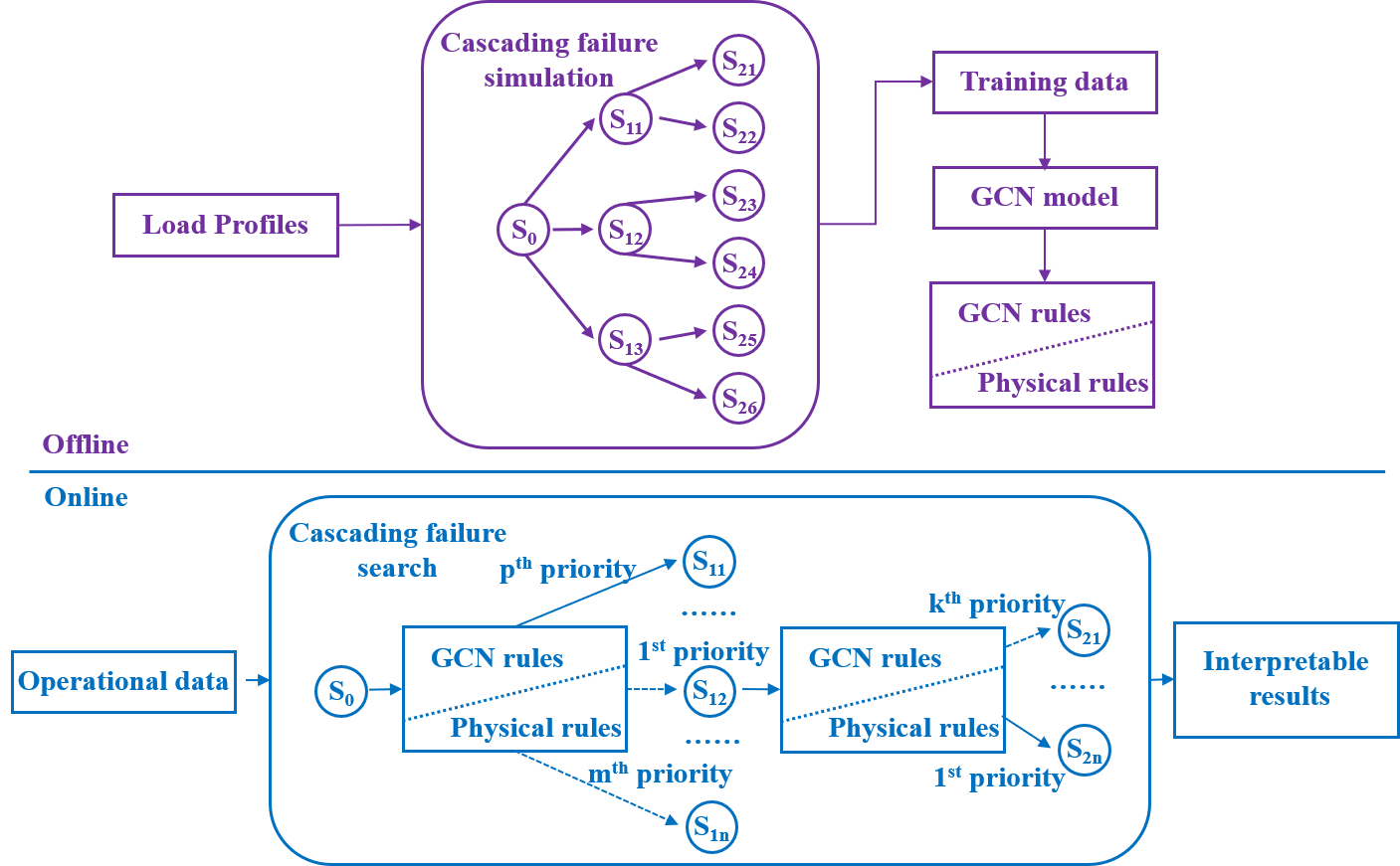
Figure 1: The framework of power system cascading failure search over different states, $\mathbf{S}$.

II-B Power System Cascading Failures Simulation

In this work, we simulate the power system cascading failures based on the ORNL-PSerc-Alaska (OPA) [25, 26] model, which is widely adopted and developed in [27, 7, 10, 19, 11]. The OPA model simulates the cascading failures triggered by branch failures in the power system. Two types of failures are considered. One type is caused by random events such as sagging and tree contact. The other type is triggered by the action of protection relays once the branch flow exceeds the preset threshold. In this work, we simulate a limited number of random failures (the first type), while we simulate all the protection relay actions once they happen. The OPA model applied in this work can be summarized as follows.

1. Step 1: Set a positive integer value $R$, so that we only consider the cases of no more than $R$ random failures. Run the DC optimal power flow (DCOPF) given the initial load profile.

2. Step 2: If the number of random branch failures is less than the preset value $R$, disconnect a branch. Else, end the simulation.

3. Step 3: Run the DC power flow (DCPF). Disconnect the branch that triggers the protection relays and run Step 3 again. If the network separates into islands, conduct load shedding for the islands which have a lack of generation.

4. Step 4: Re-dispatch the system with the objective to minimize the total load shedding and with the constraints of the system security rules (e.g. the branch flow constraints). Run Step 2.

Note that the OPA model is implemented as an indicative test bed, which is not the main focus of this work. We refer to [25, 26] for more details of the OPA model.

II-C Branch Vulnerabilities to Guide the Search

When simulating the cascading failures, the major computational burden comes from the combinatorial explosion in Step 2, i.e., we have to disconnect every branch that may fail and simulate every possible case. To ease the computational burden, we train a model that guide the search in Step 2. That is, we provide a priority on the search order at Step 2, given the current operational state. To this end, we organize the data into input $\bm{X}^{GCN}$ and output $\bm{y}^{GCN}$ to train the GCN model.

$$\bm{y}^{GCN}=f(\bm{X}^{GCN})$$ (1)

The input is the current operational state and the output is a boolean vector that quantifies the vulnerability of the branches. The $k$th variable of the vector $y^{GCN}_{k}$ is a binary value representing whether the load shedding occurs after disconnecting branch $k$ (0-without load shedding, 1-load shedding).

Afterwards, we adopt some physical rules to assist the GCN model. We calculate the value of line outage distribution factors (LODF) [28, 29]. For a system with $N$ buses, we have:

$$D_{m}^{k}=\frac{X_{m}^{k}/x_{m}}{1-X_{k}^{k}/x_{k}},\text{ }X_{m}^{k}=\mathbf{M_{m}^{T}}\mathbf{X}\mathbf{M_{k}},$$ (2)

where $D_{m}^{k}$ denotes the additional branch flow in branch $m$ (as a fraction of the initial branch flow in branch $k$) after the outage of branch $k$, $x_{k}$ is the branch reactance of branch $k$, $\mathbf{X}$ is the $N\times N$ nodal reactance matrix, and $\mathbf{M_{k}}$ is a $N\times 1$ vector for branch $k$ from bus $i$ to bus $j$:

$$\mathbf{M_{k}}={{\left[\underset{1}{\mathop{0}}\,\text{ }...\text{ }\underset{i}{\mathop{\text{1}}}\,\text{ }...\text{ }\underset{j}{\mathop{\text{-1}}}\,\text{ }...\text{ }\underset{N}{\mathop{\text{0}}}\,\right]}^{T}}.$$ (3)

After the outage of branch $k$, the vulnerability of branch $k$ can be quantified by the total branch flow in branch $m$ as a fraction of its long term maximum branch flow $L_{m}^{max}$:

$${\alpha}_{m}^{k}=|L_{m}+D_{m}^{k}L_{k}|/L_{m}^{max}$$ (4)

When ${\alpha}_{m}^{k}$ exceeds the protection relay threshold $\beta$, the protection relay will disconnect the branch $m$. When the system separates into islands, the denominator of (2) ($1-X_{k}^{k}/x_{k}$) is 0. In this case, we set $\alpha_{m}^{k}$ to another value to avoid numerical problem. We set $\alpha_{m}^{k}=\beta$ because $\beta$ already reaches the threshold to trigger the protection relays after the power flow redistribution, which is large enough to represent the vulnerability of branch $k$.

$$\begin{aligned} \hat{\alpha}_{m}^{k}=\left\{\begin{matrix}{\alpha}_{m}^{k}&1-X_{k}^{k}/x_{k}\neq 0\\ \beta&1-X_{k}^{k}/x_{k}=0\\ \end{matrix}\right.\end{aligned}.$$ (5)

Then, we define the vulnerability vector based on physical rules as $\bm{y}^{P}$, with the $k$th variable as:

$$y_{k}^{P}=\underset{m}{\mathop{\max}}\hat{\alpha}_{m}^{k}.$$ (6)

(5)-(6) denotes that the protection relay (of branch $m$ with the largest $\hat{\alpha}_{m}^{k}$) will take action or the system will separate once $y_{k}^{P}$ exceeds $\beta$. Larger $y_{k}^{P}$ intuitively implies the failure of branch $k$ maybe more likely to incur load shedding. Hence, $y_{k}^{P}$ serves as a fast yet not accurate factor to quantify the branch vulnerabilities. Finally, we guide the online search of cascading failures by both the vulnerabilities learned by the GCN $\bm{y}^{GCN}$ and the vulnerabilities from physical rules $\bm{y}^{P}$.

II-D The Online Search Algorithm

Algorithm 1 The Online Search Algorithm

1:  Step 1*: Run the DCOPF given the initial load profile;

2:  Step 2*: Use the GCN and physical rules to guide the search;

3:  while the number of random branch failures is less than a preset value $R$, do

4:     calculate $\bm{y}^{GCN}$ with (1);

5:     for all $y_{k}^{GCN}=1$, do

6:        disconnect the branch $k$ and run the Step 3 and Step 4 of the OPA model in Section II-B; run Step 2* to simulate the next failure;

7:     end for

8:     calculate $\bm{y}^{P}$ with (2)-(6);

9:     for all $y_{k}^{P}$ from the largest to the smallest, do

10:        disconnect the branch $k$ and run the Step 3 and Step 4 of the OPA model in Section II-B; run Step 2* to simulate the next failure;

11:     end for

12:  end while

13:  Step 3*: Output all the cascading paths that cause load shedding.

The online search model only differs from the OPA model in the term of the order to disconnect the branches in Step 2, so that we can detect the cascading failures that result in load shedding more efficiently. That is, we calculate the $\bm{y}^{GCN}$ and $\bm{y}^{P}$ before running Step 2. Every time we run Step 2, we first disconnect the branch that $y_{k}^{GCN}=1$, then we disconnect the branch from the largest $y_{k}^{P}$ to the smallest $y_{k}^{P}$. The aforementioned process is formulated in Algorithm 1.

III Graph Convolutional Network

III-A Learning on Graphs

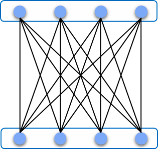
(a)

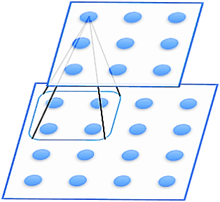
(b)

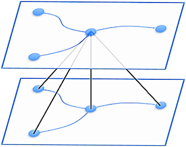
(c)

Figure 2: A demonstration of three types of layers. (a) The fully connected layer in DNN model. (b) The convolutional layer in CNN model. (c) The graph convolutional layer in GCN model.

We focus on how to build the model that maps from the current operational state to the vulnerability of the branches, as formulated in (1). The operational data of the power system is physically represented and correlated in the form of graphs. The mechanism of cascading failures is also closely related to the graphical structure of the system. Therefore we choose the GCN model over the DNN model [14] and the CNN model [16] because it is designed to capture such graph structured mechanisms. The basic layers of the DNN model, the CNN model, and the GCN model are shown in Figure 2. The above layers consist of a group of nodes. The nodes in the next layer take the weighted summation of the nodes in the previous layer. The layers mainly differ in the way that they take the weighted summation among different range of nodes in the previous layer. The layers in DNN, CNN, and GCN take the weighted summation of all the nodes, the neighboring nodes in Euclidean domain, and the neighboring nodes in graph domain, respectively. Benefiting from the structure of the graph convolutional layer, the GCN model can better capture the dependence and relationships represented by graphs.

III-B Design of GCN Structure

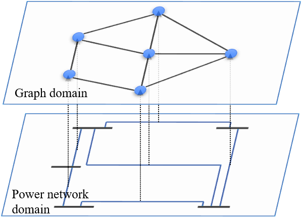
Figure 3: An illustration of the network-graph mapping, where branches in the power network are transformed to nodes in the graph.

For clarity, we use “bus” and “branch” to represent the power network, while we use “node” and “edge” to represent the graph in GCN. The traditional GCN models make classification or regression on nodes, but we search for the vulnerable branches in our framework. Hence, we conduct a network-graph mapping as demonstrated in Figure 3, where the data organized in branches is transformed to the data organized in nodes. The two nodes in the graph domain are connected when the two branches in the power network domain have common buses. For a power network with $L$ branches, the graph domain has $L$ nodes. The input of the GCN model can be formulated as:

$$\bm{X}^{GCN}=\left[\bm{x}_{1}\text{ }...\text{ }\bm{x}_{c}\text{ }...\text{ }\bm{x}_{C}\right],$$ (7)

where $C$ is the number of input features, $x_{c}$ is a $L\times 1$ vector.

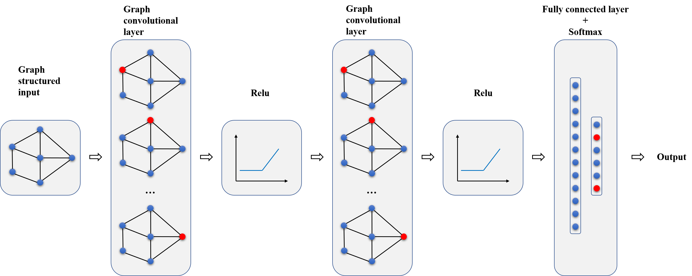
Figure 4: The structure of the proposed graph convolutional network model.

The the GCN model to guide the cascading failure search is depicted in Figure 4, which maps from $\bm{X}^{GCN}$ to $\bm{y}^{GCN}$. It consists of two graph convolutional layers and a fully connected layer with softmax output. The graph convolutional layer [23] takes the weighted average of the neighboring nodes in the graph domain and output a certain number of $L\times 1$ vectors (e.g. $F$ vectors). The $f$th output vector is given by:

$$\bm{y}_{f}^{graph}=\sum_{c=1}^{C}\mathbf{G}_{cf}\bm{x}_{c}+b_{f}\mathbf{1},$$ (8a)

$$\mathbf{G}_{cf}=\sum_{k=0}^{K}w_{cfk}\mathbf{\overline{A}}^{k},$$ (8b)

where $w_{cfk}$ is the learnable weight parameter, $b_{f}$ is the learnable constant parameter, $\mathbf{1}$ is the all-ones $L\times 1$ vector, $\mathbf{G}_{cf}$ is the $L\times L$ graph filter, $\mathbf{\overline{A}}=\mathbf{D}^{-1/2}\mathbf{A}\mathbf{D}^{-1/2}$ is the normalization of the graph adjacency matrix $\mathbf{A}$, and $\mathbf{D}$ is the diagonal degree matrix of the graph with $D_{ii}=\sum_{j}\mathbf{A}_{ij}$. Equation (8a) indicates that the output of the graph convolutional layer is the summation of inputs over graph filters. Equation (8b) indicates that the graph filter $\mathbf{G}_{cf}$ can extract the relationship within $K$ hops (or $K$ neighborhood) in a graph.

The rectified linear unit (Relu) layer serves as the activation function that add nonlinearity to the neural network. It will output the positive part of the inputs:

$$\bm{y}^{Relu}=\max(0,\bm{x}).$$ (9)

The output dimension through the graph convolutional layer and the Relu layer is $L\times F$. In one single node, the output can be transformed as a $F\times 1$ vector. We add a fully connected layer:

$$\bm{y}^{fully}=\mathbf{W}\bm{x}+b,$$ (10)

where $\mathbf{W}$ is the learnable weights parameters, and $b$ is the learnable constant parameter. In (10), $\bm{y}^{fully}$ is a $L\times 2$ vector that consists of the variables representing the conditions for each node $k$: $y_{k1}^{fully}$ for normal condition and $y_{k2}^{fully}$ for load shedding. The classification result is either normal condition or load shedding that with larger value of $y_{ki}^{fully}$.

We then introduce the softmax function to provide the probability of the final classification result:

$$y_{ki}^{soft}=\frac{e^{y_{ki}^{fully}}}{e^{y_{k1}^{fully}}+e^{y_{k2}^{fully}}}\text{, }i=1,2.$$ (11)

The classification error is set as the negative log-likelihood (NLL):

$$L^{nll}_{k}\!=-\!w_{1}y^{GCN}_{k}\!\log y_{k1}^{soft}\!-\!w_{2}(1\!-\!y^{GCN}_{k})\log y_{k2}^{soft},$$ (12)

where $L^{nll}_{k}$ is the NLL of the $k$th output, $y^{GCN}_{k}$ is the ground truth output as introduced in (1), and $w_{1}$ and $w_{2}$ are the weights to different classes. As the output has less value-1 (load shedding) than value-0 (without load shedding), we assign $w_{1}>w_{2}$ to learn from biased sample.

III-C The Parameter Space of GCN

We analyze the parameter space required to learn the cascading failure mechanism, by comparing the basic layers of the DNN model, the CNN model, and the GCN model again. The comparison of the parameter space of the fully connected layer in the DNN model, the convolutional layer in the CNN model, and the graph convolutional layer in the GCN model are shown in Table I. We assume the number of neurons of the fully connected layer is $N_{DNN}$, the kernel size of the convolutional layer is $K_{CNN}\times K_{CNN}$, and the number of hops of the graph convolutional layer is $K_{GCN}$. See [14, 16] for modeling details of the DNN and the CNN, respectively.

TABLE I: The Parameter Space of Three Types of Layers.

	Fully connected	Convolutional	Graph convolutional
Parameter space	$O(N_{DNN}^{2})$	$O(K_{CNN}^{2})$	$O(K_{GCN})$

In Table I, $N_{DNN}$ is proportional to the number of buses in a power system. $K_{CNN}$ and $K_{GCN}$ denotes how many neighboring nodes to extract the feature from, which is far less than the number of $N_{DNN}$. The neighboring nodes in convolutional layers may not be the neighboring buses in the power network, thus $N_{CNN}$ should be larger than $N_{GCN}$ to extract the feature of neighboring buses. To sum up, regarding the cascading failure learning problem, the graph convolutional layer has the smallest feature space that is efficient to train.

III-D Interpretability of the Model

To increase the interpretability of the proposed GCN model, we firstly tailor the input of our model into four parts with physical interpretations, and then we calculate the contribution factors of the inputs by an LRP algorithm.

In detail, the input of the model is a $L\times 4$ matrix:

$$\bm{X}^{GCN}=\left[\bm{x}^{t}\text{ }\bm{x}^{p}\text{ }\bm{x}^{b}\text{ }\bm{x}^{l}\right].$$ (13)

In (13), $\bm{x}^{t}$ is a boolean vector that represents the effects of current system topology (or the initial failures) on the cascading failures, with 0 for operational state and 1 for outage of a branch; $\bm{x}^{p}$ is a vector that represents the effects of protection relays, the value is the ratio of absolute branch flow to the protection relay threshold branch flow (the $k$th value is $L_{k}/\beta L_{k}^{max}$); $\bm{x}^{b}$ is the absolute branch flow vector; and $\bm{x}^{l}$ represents the larger load value between the two buses that the branch connected to. So far, we have organized our inputs into four aspects: topology, protection relay, branch flow, and the bus load.

To quantify the contribution factors of these four inputs, we implement the LRP algorithm that was proposed to explain the CNN model [30]. The LRP decomposes the output value into a combination of the model inputs. The decomposed values, a.k.a. the relevance scores, quantify the contribution of the inputs to the output. The process transforms the relevance scores of the next layer $R_{i}^{d+1}$ to the relevance scores of the previous layer $R_{i}^{d}$, such that the sum of each relevance scores of each layer equals to the output value:

$$y=\cdots=\!\!\!\!\sum_{i\in layer_{d+1}}\!\!\!\!R_{i}^{d+1}=\!\!\!\!\sum_{i\in layer_{d}}\!\!\!\!R_{i}^{d}=\cdots=\!\!\!\!\sum_{i\in layer_{1}}\!\!\!\!R_{i}^{1}.$$ (14)

We decompose the relevance scores of the next layer by the weights of the positive inputs $z_{ij}^{+}$ from all the connected neurons of the previous layer:

$$R_{i}^{d}=\sum_{j\in i}\frac{z_{ij}^{+}}{\sum_{i^{\prime}\in j}z_{i^{\prime}j}^{+}}R_{j}^{d+1},$$ (15)

where $\sum_{j\in i}$ sums over the neurons in layer $d+1$ that connected with neuron $i$, $\sum_{i^{\prime}\in j}$ sums over the neurons in layer $d$ that connected with neuron $j$, and $z_{ij}^{+}=\max(x_{i}w_{ij},0)$ is the positive part of the input from neuron $i$ to neuron $j$. We decompose the relevance scores by the weight of positive parts to compute the excitatory effects on the output of each layer. Recall that the Relu activation function only output the positive parts of the input, so that only positive input can contribute to larger output (or have excitatory effects) of the Relu activation function. We only compute the excitatory effects to focus on the factors that incurs the load shedding. In this work, we calculate the relevance scores corresponding to the output that determines the prediction of load shedding. For example, we calculate the factors that incurs the load shedding after the failure of branch $k$. In this case, according to the proposed GCN model, we decompose the output corresponding to the load shedding prediction, which is $y_{k1}^{fully}$. That is, the $y$ in (14) is $y_{k1}^{fully}$ in (10).

IV Case Studies

IV-A IEEE RTS-79 Test System

The IEEE RTS-79 test system contains 24 buses and 38 branches with a peak load of 2850 MW and a total generation capacity of 3405 MW [31]. 8000 scenarios (the $\bm{X}^{GCN}\sim\bm{y}^{GCN}$ pair described in (1)) are generated as the training dataset, to consider the cases of different load profiles and different initial contingencies. To model the load uncertainty, we multiply a random factor drawn uniformly over the interval [0.9, 1.1] to the load of every bus. To simulate a more severe result, the actual load of each scenarios from [31] is enlarged by a factor of 1.1. In this work, we consider N-2 contingencies as the random initial failures. The simulation of cascading failures is carried out based on MATLAB 2018b, Cplex 12.9 [32], and Matpower 6.0 [33]. The proposed GCN model is implemented by Pytorch 1.3 [34]. The hyper-parameters of the GCN model are tuned by 20% of the training data. We set the number of hops $K=3$, the ratio of training weight $w_{1}/w_{2}=20$, and the number of the output vectors of the first and the second graph convolutional layer as $F_{1}=16$ and $F_{2}=4$, respectively. The model is trained with 20 epochs and a batch size of 32, using the Adam optimizer [35] with the learning rate of 0.005.

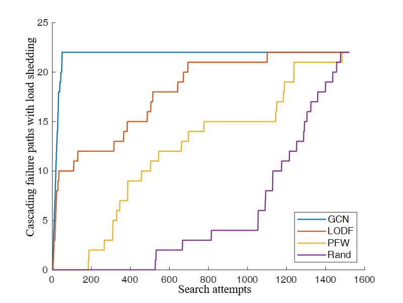
Figure 5: The number of detected cascading failure paths that incurs load shedding as a function of search attempts: the case of IEEE RTS-79 test system.

We implement a set of newly generated load profiles to test different cascading failure online search methods. Each compared method only differs from the Algorithm 1 in the orders to disconnect the branches in Step 2*.

1. Rand: The branches are disconnected randomly;

2. PFW: The branches are disconnected from the largest power flow value to the smallest power flow value. It is the deterministic form of the power flow weighted method proposed in [19];

3. LODF: The branches are disconnected by the value of $\bm{y}^{P}$ described in (2)-(6), from the largest value to the smallest value. The LODF-based method and its derivatives are widely used to search the cascading failures [10, 13]

4. GCN: Algorithm 1 proposed in this work.

We present the number of detected cascading failure paths that incurs load shedding in Figure 5. After exhaustive search, there are 22 cascading failure paths that incur load shedding. The proposed GCN method can detect all the paths after only 50 search attempts, while method LODF, PFW, and Rand detect all the paths after 1101, 1485, and 1477 search attempts, respectively. Hence, the proposed GCN method has clearly higher search efficiency than all other compared methods.

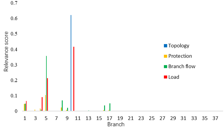
(a)

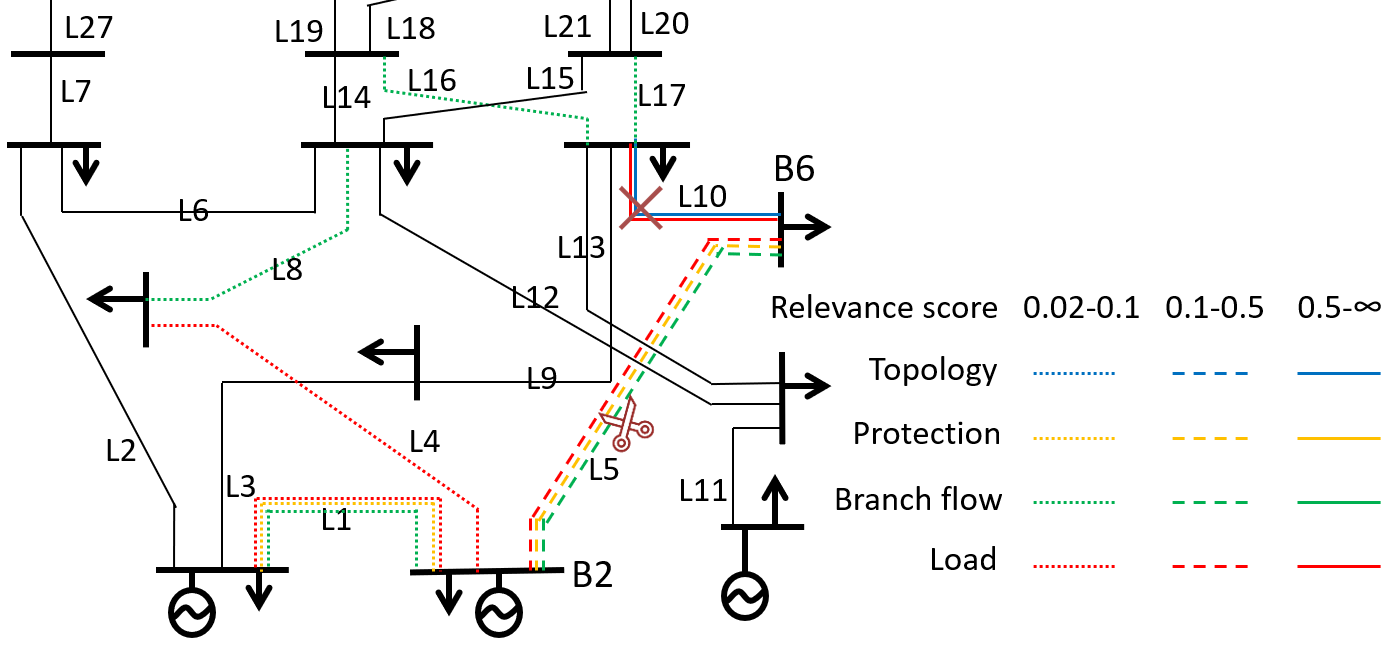
(b)

Figure 6: The relevance scores for each inputs of the GCN model that triggers the load shedding for the initial failures L10$\rightarrow$L5. (a) The bar graph. (b) The topological graph that represents a part of the IEEE RTS-79 system.

We then show the interpretability of the model by the proposed LRP method, which present the relevance scores of the inputs to a certain output. The relevance scores are the contribution factors of the inputs to the load shedding events. We use ‘L’ for branch and ‘B’ for bus. From the above 22 cascading failure paths, we analyze the case with initial failures L10$\rightarrow$L5. That is, we show the relevance scores to the 5th output of vector $\bm{y}^{GCN}$, under the power system states where L10 is already disconnected, as is depicted in Figure 6. A direct physical explanation of the load shedding is that the disconnection of L10 and L5 will result in the islanding and load shedding of B6. The relevance scores in Figure 6 can well explain the above inference. The load shedding in this case mainly results from the initial failure of L10 (the topology of L10), the increasing load of B6 (the load corresponding to L5 and L10), and the increasing branch flow from B2 to B6 (the branch flow of L5). Note that some factors are not directly related to the load shedding, but they are related to the factors that directly cause the load shedding. For example, the protection of L5 is not directly related to the load shedding of B6, but the increase of the branch flow / protection threshold ratio is closely related with the branch flow of L5. We cannot simply remove the protection vector $\bm{x}^{p}$ from the inputs, because it will serve as an independent determinant as will be shown in the next case.

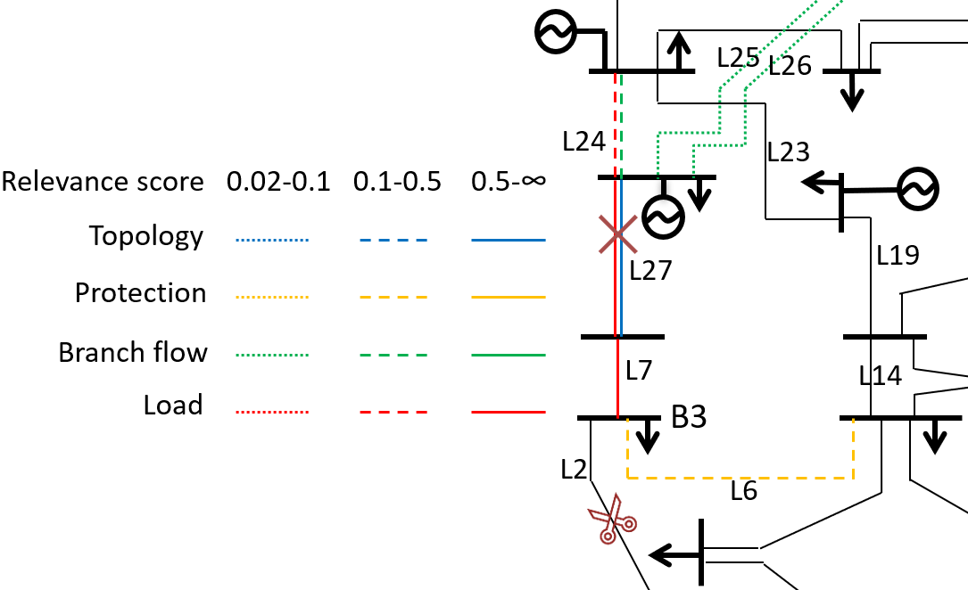
Figure 7: The relevance scores for each inputs of the GCN model that triggers the load shedding for the initial failures L27$\rightarrow$L2. The topology is only a part of the IEEE RTS-79 system.

The above interpretation results can be directly inferred from the topology of the system. To further demonstrate the interpretability of the LRP algorithm, we analyze a cascading failures case that is less apparent. The relevance scores to the 2nd output of vector $\bm{y}^{GCN}$, under the power system states that L27 is already disconnected (L27$\rightarrow$L2), is depicted in Figure 7. The disconnection of L27 and L2 will not trigger any islanding conditions, but the load in B3 relies only on the transmission line of L6. The branch flow of L6 will exceed the maximum value. Subsequently, the re-dispatching process will decrease the branch flow of L6 and causes the load shedding of B3. The relevance scores in Figure 7 can also well explain this process. The load shedding in this case mainly results from the initial failure of L27 (the topology of L27), the increasing load of B3 (the load corresponding to L7), and the branch flow limits of L6 (the protection of L6). The above cases show that the major contribution factors of the prediction results correspond to the physical inference of the cascading failures. The interpretation method can explore some less obvious factors (e.g. the protection of L6 in Figure 7) that incurs the load shedding. Still, the contribution factors also includes some indirect factors (e.g. the protection of L5 in Figure 6), which suggests that operators should be more careful or should update the model when the operation pattern changes.

IV-B The Power System of Henan Province

The power system of Henan province considered in this work is a 500kV-220kV power system. After external network equivalence, the power system contains 730 buses and 1571 branches. To consider a more severe circumstance, we enlarge the actual load profiles of Henan province by a factor of 1.1, and we reduce all the maximum branch flow thresholds by a factor of 0.8. Since the load shedding events are more rare in the Henan province case, we increase the ratio of training weight to $w_{1}/w_{2}=800$. 50000 scenarios are generated as the training dataset to model different load profiles and different initial contingencies. The model is trained with 40 epochs and a batch size of 256. All other experiment settings, including the cascading failures data generation and the model training processes, are the same with the IEEE RTS-79 test system.

We first use the power system of Henan province to test the prediction accuracy of the proposed GCN model, compared to the DNN and CNN model mentioned above. We generate 10000 new scenarios as the testing dataset. The DNN, CNN, and the GCN models are trained and tested under the same training and testing datasets, respectively. The DNN model has three fully connected layers with $4L$, $L$, and $L$ output neurons, respectively. The CNN model has two convolutional layers with one fully connected layer. The kernel size of the two convolutional layers are $3\times 3\times 16$ and $3\times 3\times 4$, respectively. All of the models implement the Relu activation function. Since the number of samples from different classes is unbalanced, a high total prediction accuracy may not be conducive to an efficient search of cascading failures. We therefore implement different indexes to evaluate the prediction result. We first introduce the confusion matrix in Table II.

TABLE II: The confusion matrix.

		Predicted results
		without load shedding	load shedding
Actual results	without load shedding	a	b
	load shedding	c	d

Several indexes are introduced [36]:

1. Total accuracy: $(a+d)/(a+b+c+d)$;

2. Hit rate: $d/(b+d)$;

3. Cover rate: $d/(c+d)$;

TABLE III: The comparison of DNN, CNN, and GCN models.

	DNN	CNN	GCN
Total accuracy	0.9416	0.9844	0.9988
Hit rate	0.0080	0.0279	0.3013
Cover rate	0.9460	0.8963	0.9961

The calculated values of the above indexes of DNN, CNN, and GCN model are listed in Table III. Note that the prediction of the load shedding events is not the final result, but acts as a guidance for the search for cascading failures that will be implemented by physical models, as shown in Algorithm 1. The total accuracy reflects the prediction results of both the cases with and without load shedding. In practice, however, the prediction of load shedding events is more related to the search efficiency of cascading failures. The hit rate measures how well the predicted load shedding events hit the actual load shedding. The cover rate is the ratio of predicted load shedding events to all the load shedding events. A small hit rate will result in useless search attempts, while a small cover rate will miss some cascading failure events so that many additional search attempts are required to compensate for the missing events. From Table III, the proposed GCN model has the best performance not only in the total accuracy, but also in terms of the hit rate and the cover rate.

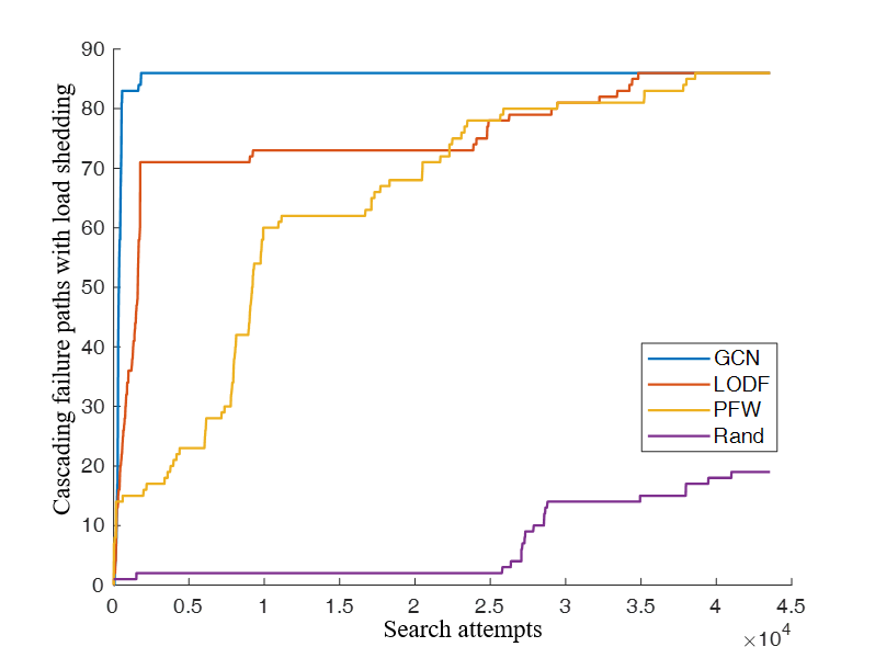
Figure 8: The number of detected cascading failure paths that incurs load shedding as a function of search attempts: the case of Henan provence power system.

Next, we present the search efficiency on a set of new load profiles of the power system of Henan province. The search performance of method Rand, PFW, LODF, and GCN are shown in Figure 8. An exhaustive search identifies 86 cascading failure paths that incur load shedding. The proposed GCN method can detect all the paths after 2160 search attempts, while methods LODF and PFW detect all the paths after $34822$ and $38608$ search attempts, respectively. Method Rand can only find a small proportion of all the paths in the given search attempts. The LODF and the PFW method have a high search efficiency at the first few search attempts, but require a high number of search attempts to detect the remaining cascading failure paths that incur load shedding. This is because some of the load shedding events can be easily detected by the physical rules (e.g. the islanding conditions), while the rest of the events are complex and cannot be detected by explicit physical rules. The above results indicate that the proposed GCN based method has a high efficiency in searching for the load shedding events caused by cascading failures.

V Conclusions

Our work provides a GCN based approach to conduct online search for the power system cascading failures with high efficiency. The proposed method links the power network topology with the structure of neural networks and therefore yeilds a smaller parameter space to predict the load shedding events caused by cascading failures. We also provide an LRP algorithm to uncover the reasons for predicting the cascading failure events. Case studies on the IEEE RTS-79 test system and on China’s Henan province power system validate the superiority of the method: 1) the GCN model has a better prediction accuracy than benchmark neural network models; 2) the GCN based cascading search method has a higher efficiency in detecting the load shedding events caused by cascading failures; 3) the prediction results of the GCN model are interpretable, enabling the user to check the logic of the model and uncover the factors that cause the cascading failures. Overall, the proposed method enables an efficient and interpretable online cascading failure search that can contribute to a reliable operation of power systems.

References

- [1] M. Vaiman, K. Bell, Y. Chen, B. Chowdhury, I. Dobson, P. Hines, M. Papic, S. Miller, and P. Zhang, “Risk assessment of cascading outages: Methodologies and challenges,” IEEE Transactions on Power Systems, vol. 27, no. 2, p. 631, 2012.
- [2] D. Bienstock, Electrical transmission system cascades and vulnerability: an operations research viewpoint. SIAM, 2015, vol. 22.
- [3] H. Haes Alhelou, M. E. Hamedani-Golshan, T. C. Njenda, and P. Siano, “A survey on power system blackout and cascading events: Research motivations and challenges,” Energies, vol. 12, no. 4, p. 682, 2019.
- [4] M. H. Athari and Z. Wang, “Impacts of wind power uncertainty on grid vulnerability to cascading overload failures,” IEEE Transactions on Sustainable Energy, vol. 9, no. 1, pp. 128–137, 2017.
- [5] Q. Chen and L. Mili, “Composite power system vulnerability evaluation to cascading failures using importance sampling and antithetic variates,” IEEE transactions on power systems, vol. 28, no. 3, pp. 2321–2330, 2013.
- [6] P. Henneaux and P.-E. Labeau, “Improving monte carlo simulation efficiency of level-i blackout probabilistic risk assessment,” in 2014 International Conference on Probabilistic Methods Applied to Power Systems (PMAPS). IEEE, 2014, pp. 1–6.
- [7] J. Kim, J. A. Bucklew, and I. Dobson, “Splitting method for speedy simulation of cascading blackouts,” IEEE Transactions on Power Systems, vol. 28, no. 3, pp. 3010–3017, 2012.
- [8] S.-P. Wang, A. Chen, C.-W. Liu, C.-H. Chen, J. Shortle, and J.-Y. Wu, “Efficient splitting simulation for blackout analysis,” IEEE Transactions on Power Systems, vol. 30, no. 4, pp. 1775–1783, 2014.
- [9] M. J. Eppstein and P. D. Hines, “A “random chemistry” algorithm for identifying collections of multiple contingencies that initiate cascading failure,” IEEE Transactions on Power Systems, vol. 27, no. 3, pp. 1698–1705, 2012.
- [10] R. Yao, S. Huang, K. Sun, F. Liu, X. Zhang, S. Mei, W. Wei, and L. Ding, “Risk assessment of multi-timescale cascading outages based on markovian tree search,” IEEE Transactions on Power Systems, vol. 32, no. 4, pp. 2887–2900, 2016.
- [11] Y. Liu, Y. Wang, P. Yong, N. Zhang, C. Kang, and D. Lu, “Fast power system cascading failure path searching with high wind power penetration,” IEEE Transactions on Sustainable Energy, 2019.
- [12] S. Soltan, D. Mazauric, and G. Zussman, “Analysis of failures in power grids,” IEEE Transactions on Control of Network Systems, vol. 4, no. 2, pp. 288–300, 2015.
- [13] S. Soltan, A. Loh, and G. Zussman, “Analyzing and quantifying the effect of -line failures in power grids,” IEEE Transactions on Control of Network Systems, vol. 5, no. 3, pp. 1424–1433, 2017.
- [14] F. Li and Y. Du, “From alphago to power system ai: What engineers can learn from solving the most complex board game,” IEEE Power and Energy Magazine, vol. 16, no. 2, pp. 76–84, 2018.
- [15] Y. Du, F. F. Li, J. Li, and T. Zheng, “Achieving 100x acceleration for n-1 contingency screening with uncertain scenarios using deep convolutional neural network,” IEEE Transactions on Power Systems, 2019.
- [16] J.-M. H. Arteaga, F. Hancharou, F. Thams, and S. Chatzivasileiadis, “Deep learning for power system security assessment,” in 13th IEEE PowerTech 2019. IEEE, 2019.
- [17] M. Sun, I. Konstantelos, and G. Strbac, “A deep learning-based feature extraction framework for system security assessment,” IEEE Transactions on Smart Grid, 2018.
- [18] J. Yan, H. He, X. Zhong, and Y. Tang, “Q-learning-based vulnerability analysis of smart grid against sequential topology attacks,” IEEE Transactions on Information Forensics and Security, vol. 12, no. 1, pp. 200–210, 2016.
- [19] Z. Zhang, S. Huang, Y. Chen, S. Mei, R. Yao, and K. Sun, “An online search method for representative risky fault chains based on reinforcement learning and knowledge transfer,” IEEE Transactions on Power Systems, 2019.
- [20] P. D. Hines, I. Dobson, and P. Rezaei, “Cascading power outages propagate locally in an influence graph that is not the actual grid topology,” IEEE Transactions on Power Systems, vol. 32, no. 2, pp. 958–967, 2016.
- [21] J. Cremer, I. Konstantelos, and G. Strbac, “From optimization-based machine learning to interpretable security rules for operation,” IEEE Transactions on Power Systems, 2019.
- [22] Z. Wu, S. Pan, F. Chen, G. Long, C. Zhang, and P. S. Yu, “A comprehensive survey on graph neural networks,” arXiv preprint arXiv:1901.00596, 2019.
- [23] J. Du, S. Zhang, G. Wu, J. M. Moura, and S. Kar, “Topology adaptive graph convolutional networks,” arXiv preprint arXiv:1710.10370, 2017.
- [24] F. Baldassarre and H. Azizpour, “Explainability techniques for graph convolutional networks,” arXiv preprint arXiv:1905.13686, 2019.
- [25] B. A. Carreras, V. E. Lynch, I. Dobson, and D. E. Newman, “Complex dynamics of blackouts in power transmission systems,” Chaos: An Interdisciplinary Journal of Nonlinear Science, vol. 14, no. 3, pp. 643–652, 2004.
- [26] H. Ren, I. Dobson, and B. A. Carreras, “Long-term effect of the n-1 criterion on cascading line outages in an evolving power transmission grid,” IEEE transactions on power systems, vol. 23, no. 3, pp. 1217–1225, 2008.
- [27] S. Mei, F. He, X. Zhang, S. Wu, and G. Wang, “An improved opa model and blackout risk assessment,” IEEE Transactions on Power Systems, vol. 24, no. 2, pp. 814–823, 2009.
- [28] T. Guler, G. Gross, and M. Liu, “Generalized line outage distribution factors,” IEEE Transactions on Power Systems, vol. 22, no. 2, pp. 879–881, 2007.
- [29] D. A. Tejada-Arango, P. Sánchez-Martın, and A. Ramos, “Security constrained unit commitment using line outage distribution factors,” IEEE Transactions on Power Systems, vol. 33, no. 1, pp. 329–337, 2017.
- [30] S. Bach, A. Binder, G. Montavon, F. Klauschen, K.-R. Müller, and W. Samek, “On pixel-wise explanations for non-linear classifier decisions by layer-wise relevance propagation,” PloS one, vol. 10, no. 7, p. e0130140, 2015.
- [31] Probability Methods Subcommittee, “IEEE reliability test system,” IEEE Trans. power apparatus and systems, no. 6, pp. 2047–2054, 1979.
- [32] T. S. Manuals, “Cplex document,” https://www.ibm.com/products/ilog-cplex-optimization-studio, 2019.
- [33] R. D. Zimmerman, C. E. Murillo-Sánchez, and R. J. Thomas, “Matpower: Steady-state operations, planning, and analysis tools for power systems research and education,” IEEE Transactions on power systems, vol. 26, no. 1, pp. 12–19, 2010.
- [34] A. Paszke, S. Gross, F. Massa, A. Lerer, J. Bradbury, G. Chanan, T. Killeen, Z. Lin, N. Gimelshein, L. Antiga et al., “Pytorch: An imperative style, high-performance deep learning library,” in Advances in Neural Information Processing Systems, 2019, pp. 8024–8035.
- [35] D. P. Kingma and J. Ba, “Adam: A method for stochastic optimization,” arXiv preprint arXiv:1412.6980, 2014.
- [36] D. M. Powers, “Evaluation: from precision, recall and f-measure to roc, informedness, markedness and correlation,” 2011.