Global $\mathbb{T}$ Operator Bounds on Electromagnetic Scattering:
Upper Bounds on Far-Field Cross Sections

Abstract

We present a method based on the scattering $\mathbb{T}$ operator, and conservation of net real and reactive power, to provide physical bounds on any electromagnetic design objective that can be framed as a net radiative emission, scattering or absorption process. Application of this approach to planewave scattering from an arbitrarily shaped, compact body of homogeneous electric susceptibility $\chi$ is found to predictively quantify and differentiate the relative performance of dielectric and metallic materials across all optical length scales. When the size of a device is restricted to be much smaller than the wavelength (a subwavelength cavity, antenna, nanoparticle, etc.), the maximum cross section enhancement that may be achieved via material structuring is found to be much weaker than prior predictions: the response of strong metals ($\operatorname{Re}\left[\chi\right]\ll 0$) exhibits a diluted (homogenized) effective medium scaling $\propto\left|\chi\right|/\operatorname{Im}\left[\chi\right]$; below a threshold size inversely proportional to the index of refraction (consistent with the half-wavelength resonance condition), the maximum cross section enhancement possible with dielectrics ($\operatorname{Re}\left[\chi\right]>0$) shows the same material dependence as Rayleigh scattering. In the limit of a bounding volume much larger than the wavelength in all dimensions, achievable scattering interactions asymptote to the geometric area, as predicted by ray optics. For representative metal and dielectric materials, geometries capable of scattering power from an incident plane wave within an order of magnitude (typically a factor of two) of the bound are discovered by inverse design. The basis of the method rests entirely on scattering theory, and can thus likely be applied to acoustics, quantum mechanics, and other wave physics.

Much of the continuing appeal and challenge of linear electromagnetics stems from the same root: given some desired objective (enhancing radiation from a quantum emitter Eggleston et al. [2015], Aharonovich et al. [2016], Liu et al. [2017], Koenderink [2017], Cox et al. [2018], the field intensity in a photovoltaic Mokkapati and Catchpole [2012], Sheng et al. [2012], Ganapati et al. [2013], the radiative cross section of an antenna Shahpari and Thiel [2018], Capek et al. [2019], Wientjes et al. [2014], etc.) subject to some practical constraints (material compatibility Selvaraja et al. [2009], Briggs et al. [2016], Roberts et al. [2018], fabrication tolerances Lazarov et al. [2016], Boutami and Fan [2019], Vercruysse et al. [2019], or device size Ourir et al. [2006], Law et al. [2004], Caldwell et al. [2014]), there is currently no method for finding uniquely best solutions. The associated difficulties are well known Ahn et al. [1998], Polimeridis et al. [2014], Pestourie et al. [2018]. From plasmonic resonators Friedler et al. [2009], Santhosh et al. [2016], Chou et al. [2018] to periodic lattices Boroditsky et al. [1999], Lu et al. [2016], Yu et al. [2017], myriad combinations of materials and geometries can be used to manipulate electromagnetic characteristics (enhancing interactions with matter Gröblacher et al. [2009], Tang and Cohen [2010], Koenderink et al. [2015], Bliokh et al. [2015], High et al. [2015], Flick et al. [2018]) in extraordinary ways, but net effects are often similar Rinnerbauer et al. [2013], Dyachenko et al. [2016]. The wave nature of Maxwell’s equations and non-convexity of electromagnetic optimizations with respect to material susceptibility makes discerning optimal solutions challenging Boyd and Vandenberghe [2004], Angeris et al. [2019], Jiang and Fan [2019], often leading to the consideration of designs that are sensitive to minute structural alterations Im et al. [2014], Gandhi et al. [2019]. In most situations of practical interest, quantitative relations between basic design characteristics (like available volume and material response) and achievable performance are not known.

Figure 1: Schematic of investigation. To what extent does the specification of an electric susceptibility ($\chi$) and a confining spatial domain for the design of a structured body (optical device), determine the maximum absorbed $P_{\text{abs}}$, scattered $P_{\text{sct}}$, and extinguished (total) $P_{\text{ext}}=P_{\text{sct}}+P_{\text{abs}}$ power that can be extracted from a known incident field?

Nevertheless, despite these apparent challenges, computational (inverse) design techniques based on local gradients have proven to be impressively successful Jensen and Sigmund [2011], Molesky et al. [2018], Lebbe et al. [2019], offering substantial improvements for applications such as on-chip optical routing Frellsen et al. [2016], Su et al. [2017], Lebbe et al. [2019], meta-optics  Bayati et al. [2020], Callewaert et al. [2018], Zhan et al. [2019], nonlinear frequency conversion Lin et al. [2016a], Sitawarin et al. [2018], and engineered bandgaps Men et al. [2014], Meng et al. [2018]. The widespread success of these techniques, and their increasing prevalence, begs a number of questions. Namely, how far can this progress continue, and, if salient limits do exist, can this information be leveraged to either facilitate future inverse approaches or define better computational objectives. Absent benchmarks of what is possible, precise evaluation of the merits of any design methodology or algorithm is difficult: failure to meet desired application metrics may be caused by issues in the selected objectives, the range and type of parameters investigated, or the formulation itself.

Building from similar pragmatic motivations, and basic curiosity, prior efforts to elucidate bounds on optical interactions, surveyed briefly in Sec. II, have provided insights into a diverse collection of topics, including antennas Vercruysse et al. [2014], Shahpari and Thiel [2018], Capek et al. [2019], light trapping Yablonovitch [1982], Siegel and Spuckler [1993], Yu et al. [2012], Callahan et al. [2012], Mokkapati and Catchpole [2012], Miroshnichenko and Tribelsky [2018], and optoelectronic Niv et al. [2012], Miller and Yablonovitch [2013], Xu et al. [2015], Liu et al. [2016] devices, and have resulted in improved design tools for a range of applications Munsch et al. [2013], Feichtner et al. [2017], Yang et al. [2017], Angeris et al. [2019]. Yet, their domain of meaningful applicability remains fragmented. Barring recent computational bounds established by Angeris, Vučković and Boyd Angeris et al. [2019], which are limits of a different sort, applicability is highly context dependent. Relevant arguments largely shift with circumstance Molesky et al. [2019, 2020], and even within any single setting, attributes widely recognized to affect performance (e.g., differences between metallic and dielectric materials, the necessity of conserved quantities, required boundaries, minimum feature sizes) are frequently unaccounted for, leading to unphysical asymptotics and/or bounds many orders of magnitude larger than those achieved by state-of-the-art photonic structures, Fig. 1.

In this article, we exploit the requirement of global (net) power conservation as constructed from the defining relation of the scattering $\mathbb{T}$ operator, in conjunction with Lagrange duality, to derive bounds on any electromagnetic objective equivalent to a net extinction, scattering, or absorption process. With minor modifications for cases where one is interested in only a portion of the output field Gustafsson et al. [2016], such phenomena encompass nearly every application mentioned above. The scheme, capturing the potential of any and all possible structures under the fundamental wave limitations contained in Maxwell’s equations, requires only three specified attributes: the material the device will be made of, the volume it can occupy, and the source (current or electromagnetic field) that it will interact with. Directly, the conservation of real power is seen to set an upper bound on the magnitude of a system’s net polarization response, while the analog of the optical theorem for reactive power, introducing the polarization phase, is shown to severely restrict the conditions under which resonant response is attainable, particularly in weak dielectrics (glasses), leading to significantly tighter limits compared to related works Miller et al. [2016], Kuang et al. [2020].

The utility of a more robust, methodic, approach for treating electromagnetic performance limits has been recognized by several other researchers (especially in the field of radio frequency antennas Gustafsson et al. [2016], Jelinek and Capek [2016], Gustafsson and Capek [2019]), and in particular, concurrent works by Kuang et al. Kuang et al. [2020] and Gustafsson et al. Gustafsson et al. [2020] have converged on the same basic optimization approach given in Sec. I. Although Ref. Kuang et al. [2020] considers only the conservation of real power, and thus overestimates achievable performance for certain parameter combinations (Figs. 2 and 3), the findings presented in these articles are excellent complements to our results, further highlighting the adaptability and utility of Lagrange duality and scattering theory for predicting possible performance in photonics. Moreover, during review of this article, another program for calculating bounds via the self-consistency of the total scattering field has also been put forward by Trivedi et al. Trivedi et al. [2020]. A brief description of this work, as well as those cited above, is given in Sec. II.

Application of the technique to compute limits on far-field scattering cross sections for any object of electric susceptibility $\chi$ that can be bounded by (contained in) either a ball of radius $R$ or a periodic film of thickness $t$ interacting with a plane wave of wavelength $\lambda$, codifies a substantial amount of intuition pertaining to optical devices. As $R/\lambda\rightarrow 0$, the requirement of reactive power conservation means that the energy transferred between a generated polarization current and its exciting (incident) field, averaged over the confining volume, can never scale as the material enhancement factor of $\zeta_{\text{mat}}=|\chi|^{2}/\operatorname{Im}\left[\chi\right]$ introduced and broadly discussed in prior works Miller et al. [2016], Yang et al. [2017, 2018], Michon et al. [2019], Molesky et al. [2019], Venkataram et al. [2020a], Molesky et al. [2020]. Instead, for metals ($\operatorname{Re}\left[\chi\right]\leq-3$), with $\operatorname{Re}\left[\chi\right]=-3$ corresponding to the localized plasmon-polariton resonance Novotny and Hecht [2012] of a spherical nanoparticle, the relative strength of such interactions cannot surpass, as compared to $\zeta_{\text{mat}}$, the reduced form factor $3\left|\chi\right|/\operatorname{Im}\left[\chi\right]$, consistent with a “dilution” of metallic response implied by homogenized or effective medium perspectives Liu et al. [2007], Cai and Shalaev [2010], Jahani and Jacob [2016]. When $\operatorname{Re}\left[\chi\right]>-3$, even this level of enhancement is not possible. For dielectrics ($\operatorname{Re}\left[\chi\right]>0$), enhancement is limited by the same material dependence that appears in Rayleigh scattering Hulst and van de Hulst [1981], approximately $3\left|\chi\right|/\left|\chi+3\right|$. (In either case, comparison with cross section limits based on shape dependent coupled mode or effective medium models Hamam et al. [2007], Merrill et al. [1999] reveals notable inexactness.) After surpassing a wavelength condition inversely proportional to the index of refraction, the importance of reactive power is superseded by the conservation of real power, causing $\operatorname{Re}\left[\chi\right]$ to have less drastic consequences on the magnitude of achievable cross sections; for $R\approx\lambda/2$, limits for dielectrics meet or surpass those of metals for realistic material loss values, $\operatorname{Im}\left[\chi\right]$. In the macroscopic limit of $R\gg\lambda$ or $t\gtrsim\lambda/2$, the selected material plays almost no role in setting achievable scattering cross sections, other than determining the level of structuring that would be required, and the predictions of ray optics (geometric cross sections) emerge. Additionally, beyond these asymptotic features, for representative metallic and dielectric material selections, geometries discovered through topology optimization Jensen and Sigmund [2011], Molesky et al. [2018] are shown to come within an order of magnitude of the bounds for domain sizes varying between $R/\lambda=10^{-3}$ and $R/\lambda=1$, with connate agreement for periodic films, providing supporting evidence that the bounds are nearly tight and predictive.

Figure 2: Scattering cross section bounds for a planewave incident on a compact object. The four panels show different aspects of scattering cross section bounds for any structure of electric susceptibility $\chi$ that can be contained within a spherical boundary of $R/\lambda$ (e.g., cavities, nanoparticle, etc.). Dashed lines result from imposing the conservation of real power, as in Ref. Kuang et al. [2020]. Full lines result from additionally requiring the conservation of reactive power, as in Ref. Gustafsson et al. [2020]. As $R\rightarrow 0$, limit values agree with (38) in all cases, and with (40) so long as $\operatorname{Im}\left[\chi\right]/\left|\operatorname{Re}\left[\chi\right]\right|\gtrsim 10^{-4}$. Dots in panels (a) and (b) mark scattering cross sections achieved in actual geometries discovered by inverse design, for $\chi=-10+i~{}10^{-1}$ and $\chi=16+i~{}10^{-6}$, respectively. For the metal structure in (a), vertically aligned cross-hatched dots result from enforcing binarized permittivity profiles. (Binarization does not alter the dielectric results.) Two sample structures are shown as insets, with the planewave incident from the more solid side of both designs, left side in (a), right side in (b), and aligned along the left-right symmetry axis. Unbounded cross sections are encountered only for fictitious metals with vanishing material loss, with the bounds exhibiting a weak, sub-logarithmic, divergence as $\operatorname{Im}\left[\chi\right]\rightarrow 0$. More practically, cross section enhancements surpassing $\approx 200$ should not be expected. Descriptions of other major features are given in the accompanying text.

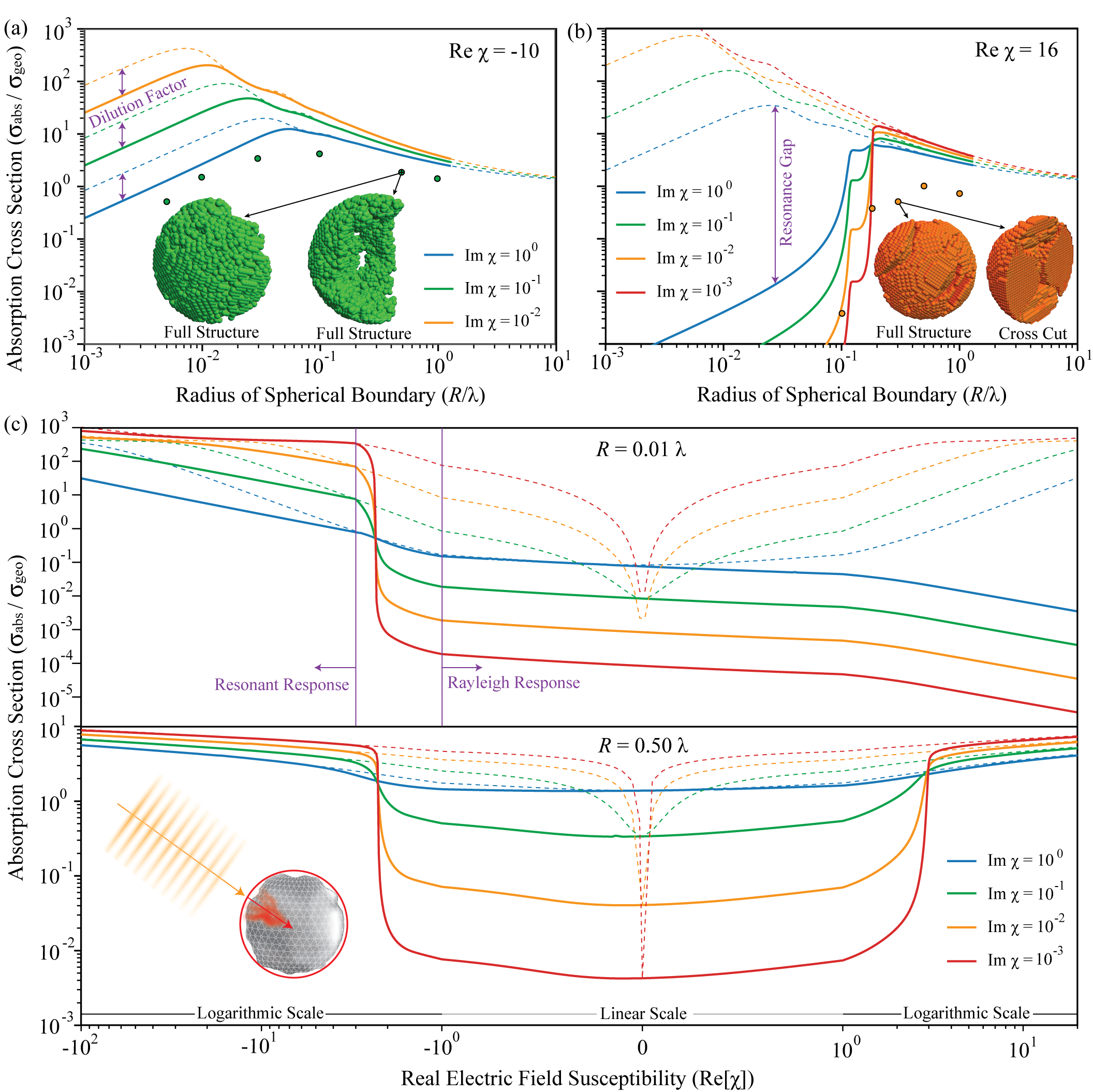
Figure 3: Absorption cross section bounds for a planewave incident on a compact object. The four panels provide analogous information as Fig. 2, but for absorbed rather than scattered power. Again, the dashed lines represent bounds determined by insisting only that real power is conserved, the solid lines result from additionally requiring the conservation of reactive power, and dots correspond to actual structures discovered by inverse design. For the example metal structure shown in (a), the planewave is incident from the solid side of the half shell (from the left in the first view and from the back left in the second). For the example dielectric structure, the planewave is incident from the left along the axis of symmetry of the mushroom cap in the full view, and from the back left in the cross cut. Small radii features are found to be in good agreement with the asymptotic predictions of (38) and (40) for $\operatorname{Im}\left[\chi\right]/\left|\operatorname{Re}\left[\chi\right]\right|\gtrsim 10^{-4}$. When the confining volume is small, $R/\lambda\lesssim 1/20$, the ability of a structured object to absorb radiation is found to be substantially weaker than past predictions Miller et al. [2016], Yang et al. [2018], Molesky et al. [2019]. As $R\rightarrow\infty$, the geometric cross section limit predicted by ray optics is recovered regardless of the material considered. Like scattering, these results indicate that absorption cross section enhancements larger than $\approx 200$ should not be expected.

These same findings also shed light on a range of fundamental questions, such as limitations for light extraction and trapping efficiency, and the relative merits of different materials for particular applications Liu et al. [2016], Jahani and Jacob [2016], Staude et al. [2019], and provide a much more quantitative perspective on which aspects of a design are most critical to device performance than prior analyses. Shortly, we foresee extensions of the framework to embedded sources and user defined design (containing) volumes as providing a means of formalizing, comparing, and contrasting existing paradigms within photonics, revealing limitations and trade offs in a number of technologically prescient areas (e.g., the radiative efficiency of quantum emitters Lu et al. [2017], Davoyan and Atwater [2018], Crook et al. [2020], high quality factor cavities Lin et al. [2016b], Liu and Houck [2017], Wang et al. [2018], optical forces  Venkataram et al. [2020b], luminescence Zalogina et al. [2018], Valenta et al. [2019] and fluorescence Li et al. [2017a], Simovski [2019]).

The article is divided into four main sections. Section I begins with an overview of the $\mathbb{T}$ operator relations governing absorption, scattering and radiative processes, followed by a statement of the wave constraints and relaxations that are explored in the rest of the manuscript. From these preliminaries, the calculations of limits is then cast in the language of optimization theory, and a solution in terms of the Lagrangian dual is given. In Sec. II, a brief examination of the similarities and differences of this approach with current art is supplied. Next, in Sec. III, basic computational mechanics are examined, and the quasistatic $R/\lambda\rightarrow 0$ scaling factors quoted elsewhere are derived based on analytically tractable single-channel asymptotics. Finally, Sec. IV provides sample applications of the method as described above. This is likely the section of the text of most relevance to the majority of readers. Although only single frequency examples are given, broad bandwidth objectives should present no major hurdles Liang and Johnson [2013], Shim et al. [2019]. Further technical details, necessary only for reproducing our results, appear in Sec. VII. Because the approach relies exclusively on the validity of scattering theory, it is likely that counterparts of the presented findings exist in acoustics, quantum mechanics, and any other wave physics.

I Formalism

The key to the approach of this article rests on the use of partial relaxations Pardalos and Romeijn [2013]. Past electromagnetic limits, including our own work, have been predominately formulated by placing bounds on the individual physical quantities entering an objective and then deducing a total bound by composing the component limits Miller [2007], Miller et al. [2015]. We begin, alternatively, with the fundamental scattering relation that any physical system must satisfy, derive algebraic consequences of this relations (e.g. energy conservation) and then suppose a subset of theses conclusions as constraints on an otherwise abstract optimization. This general procedure is detailed below. The formulas given in the Power Objectives and Scattering Constraints subsections are exact. Relaxations (omissions of certain physical requirements) begin only after the Relaxation and Optimization heading.

I.1 Power Objectives

Considerations of power transfer in electromagnetics typically belong to one of two categories: initial flux problems, wherein power is drawn from an incident electromagnetic field, and initial source problems, wherein power is drawn from a predefined current excitation. Initial flux problems are typical in scattering theory, and as such, our nomenclature follows essentially from this area Tsang et al. [2004]. That is, we will denote the initial (incident, given, or bare) field with an $i$ superscript (either $\left|\textbf{E}^{i}\right>$ or $\left|\textbf{J}^{i}\right>$) and the total (or dressed) field with a $t$ superscript. For a pair of initial and total quantities referring to the same underlying field, the scattered field, $s$ superscript, is defined as the difference $\left|\textbf{F}^{s}\right>=\left|\textbf{F}^{t}\right>-\left|\textbf{F}^{i}\right>.$ There is a certain appeal to transforming one of these two classes of problem into the other via equivalent fields. However, due to the additional back action that can occur in initial source problems, in our experience a unified framework promotes logical slips. For this reason, the total polarization field of an initial flux problem (or total electromagnetic field of an initial source problem) will be referred to as a generated field, $g$ superscript. With this notation, scattering theory for initial flux and source problems consists of the following relations:

$$\left|\textbf{J}^{g}\right> =-\frac{ik}{Z}\mathbb{V}\left|\textbf{E}^{t}\right>, \left|\textbf{E}^{t}\right> =\mathbb{V}^{-1}\mathbb{T}\left|\textbf{E}^{i}\right>,$$

$$\left|\textbf{E}^{t}\right> =\left|\textbf{E}^{i}\right>+\frac{iZ}{k}\mathbb{G}^{\text{0}}\left|\textbf{J}^{g}\right>, \left|\textbf{E}^{s}\right> =\frac{iZ}{k}\mathbb{G}^{\text{0}}\left|\textbf{J}^{g}\right>,$$ (1)

$$\left|\textbf{E}^{g}\right> =\frac{iZ}{k}\mathbb{G}^{\text{0}}\left|\textbf{J}^{t}\right>, \left|\textbf{J}^{t}\right> =\mathbb{T}\mathbb{V}^{-1}\left|\textbf{J}^{i}\right>,$$

$$\left|\textbf{J}^{t}\right> =\left|\textbf{J}^{i}\right>-\frac{ik}{Z}\mathbb{V}\left|\textbf{E}^{g}\right>, \left|\textbf{J}^{s}\right> =-\frac{ik}{Z}\mathbb{V}\left|\textbf{E}^{g}\right>.$$ (2)

Here and throughout, $\mathbb{G}^{\text{0}}$ marks the background or environmental Green function, which may or may not be vacuum Novotny and Hecht [2012]. The $\mathbb{V}$ operator refers to the scattering potential (susceptibility) relative to this background (whatever material was not included when $\mathbb{G}^{\text{0}}$ was computed), and $\left|\textbf{E}^{i}\right>$ and $\left|\textbf{J}^{i}\right>$ are similarly defined as initial fields (solutions) in the background. The remaining quantities in (1) and (2) are the impedance of free space $Z$, the wavenumber $k=2\pi/\lambda$ (with $\lambda$ the wavelength), and the $\mathbb{T}$ operator, defined by the formal equality $\mathbb{I}=(\mathbb{V}^{-1}-\mathbb{G}^{\text{0}})\mathbb{T}$ Molesky et al. [2020].

The three primary operator forms for energy transfer in an initial flux problem are the extracted power,

$$P_{\text{flx}}^{\text{ext}}=\frac{1}{2}\operatorname{Re}\left[\left<\textbf{E}^{i}|\textbf{J}^{g}\right>\right]=\frac{k}{2Z}\operatorname{Tr}\left[\mathbb{S}_{E}\operatorname{Asym}\left[\mathbb{T}\right]\right],$$ (3)

the absorbed power,

$$P_{\text{flx}}^{\text{abs}} =\frac{1}{2}\operatorname{Re}\left[\left<\textbf{E}^{t}|\textbf{J}^{g}\right>\right]=\frac{k}{2Z}\operatorname{Tr}\left[\mathbb{S}_{E}\left(\mathbb{T}^{\dagger}\operatorname{Asym}\left[\mathbb{V}^{-1\dagger}\right]\mathbb{T}\right)\right],$$

$$=\frac{k}{2Z}\operatorname{Tr}\left[\mathbb{S}_{E}\left(\operatorname{Asym}\left[\mathbb{T}\right]-\mathbb{T}^{\dagger}\operatorname{Asym}\left[\mathbb{G}^{\text{0}}\right]\mathbb{T}\right)\right],$$ (4)

and the scattered power,

$$P_{\text{flx}}^{\text{sct}} =-\frac{1}{2}\operatorname{Re}\left[\left<\textbf{E}^{s}|\textbf{J}^{g}\right>\right]=\frac{k}{2Z}\operatorname{Tr}\left[\mathbb{S}_{E}\mathbb{T}^{\dagger}\operatorname{Asym}\left[\mathbb{G}^{\text{0}}\right]\mathbb{T}\right]$$

$$=\frac{k}{2Z}\operatorname{Tr}\left[\mathbb{S}_{E}\left(\operatorname{Asym}\left[\mathbb{T}\right]-\mathbb{T}^{\dagger}\operatorname{Asym}\left[\mathbb{V}^{-1\dagger}\right]\mathbb{T}\right)\right];$$ (5)

with $\mathbb{S}_{E}=\left|\textbf{E}^{i}\right>\left<\textbf{E}^{i}\right|$ denoting projection of the corresponding operators onto the incident fields. Reciprocally, the three principal forms characterizing power flow from an initial current excitation are the extracted power,

$$P_{\text{src}}^{\text{ext}} =-\frac{1}{2}\operatorname{Re}\left[\left<\textbf{J}^{i}|\textbf{E}^{g}\right>\right]$$

$$=\frac{Z}{2k}\operatorname{Tr}\left[\mathbb{S}_{J}\left(\operatorname{Asym}\left[\mathbb{V}^{-1\dagger}\right]+\operatorname{Asym}\left[\mathbb{V}^{-1}\mathbb{T}\mathbb{V}^{-1}\right]\right)\right],$$

$$=\frac{Z}{2k}\operatorname{Tr}\left[\mathbb{S}_{J}\left(\operatorname{Asym}\left[\mathbb{G}^{\text{0}}\right]+\operatorname{Asym}\left[\mathbb{G}^{\text{0}}\mathbb{T}\mathbb{G}^{\text{0}}\right]\right)\right]$$ (6)

the radiated power,

$$P_{\text{src}}^{\text{rad}} =-\frac{1}{2}\operatorname{Re}\left[\left<\textbf{J}^{t}|\textbf{E}^{g}\right>\right]$$

$$=\frac{Z}{2k}\operatorname{Tr}\left[\mathbb{S}_{J}\left(\mathbb{V}^{-1\dagger}\mathbb{T}^{\dagger}\operatorname{Asym}\left[\mathbb{G}^{\text{0}}\right]\mathbb{T}\mathbb{V}^{-1}\right)\right]$$

$$=\frac{Z}{2k}\operatorname{Tr}\big{[}\mathbb{S}_{J}\mathbb{V}^{-1\dagger}\left(\operatorname{Asym}\left[\mathbb{T}\right]\right.-$$

$$\hskip 39.74872pt\left.\mathbb{T}^{\dagger}\operatorname{Asym}\left[\mathbb{V}^{-1\dagger}\right]\mathbb{T}\right)\mathbb{V}^{-1}\big{]}$$

$$=\frac{Z}{2k}\operatorname{Tr}\big{[}\mathbb{S}_{J}\big{(}\operatorname{Asym}\left[\mathbb{G}^{\text{0}}\right]+\operatorname{Asym}\left[\mathbb{G}^{\text{0}}\mathbb{T}\mathbb{G}^{\text{0}}\right]-$$

$$\hskip 43.36243pt\mathbb{G}^{\text{0}\dagger}\mathbb{T}^{\dagger}\operatorname{Asym}\left[\mathbb{V}^{-1\dagger}\right]\mathbb{T}\mathbb{G}^{\text{0}}\big{)}\big{]},$$ (7)

and the material (loss) power,

$$P_{\text{src}}^{\text{mat}} =\frac{1}{2}\operatorname{Re}\left[\left<\textbf{J}^{s}|\textbf{E}^{g}\right>\right]$$

$$=\frac{Z}{2k}\operatorname{Tr}\left[\mathbb{S}_{J}\left(\mathbb{G}^{\text{0}\dagger}\mathbb{T}^{\dagger}\operatorname{Asym}\left[\mathbb{V}^{-1\dagger}\right]\mathbb{T}\mathbb{G}^{\text{0}}\right)\right]$$

$$=\frac{Z}{2k}\operatorname{Tr}\big{[}\mathbb{S}_{J}\left(\mathbb{G}^{\text{0}\dagger}\operatorname{Asym}\left[\mathbb{T}\right]\mathbb{G}^{\text{0}}-\right.$$

$$\hskip 39.74872pt\left.\mathbb{G}^{\text{0}\dagger}\mathbb{T}^{\dagger}\operatorname{Asym}\left[\mathbb{G}^{\text{0}}\right]\mathbb{T}\mathbb{G}^{\text{0}}\right)\big{]},$$ (8)

with $\mathbb{S}_{J}=\left|\textbf{J}^{i}\right>\left<\textbf{J}^{i}\right|$ denoting projection of the corresponding operators onto the initial current sources. The naming of the final two forms, which appear less frequently than the other four, follows from the observation that once the total source $\left|\textbf{J}^{t}\right>$ is determined the corresponding electromagnetic field is generated exclusively via the background Green’s function. Hence, the energy transfer dynamics of a total source are exactly those of a special “free” current distribution. Because the only pathway for power to flow from a current source in free space (or lossless background) is radiative emission, $P^{\text{rad}}_{\text{src}}$ must be interpreted in this way—energy transfer into the source free solutions of the background—and similarly, $P^{\text{mat}}_{\text{src}}$ must be equated with loss into the scatterer. This reversal of forms and physics (compared absorption and scattering) is sensible from the perspective of field conversion. Absorption is the conversion of an electromagnetic field into a current, and radiative emission the conversion of a current into an electromagnetic field. Scattering in an initial flux setting is the creation of a new field of the same type, as is material loss in an initial source setting.

Note, however, that there is a caveat to these interpretations. $\mathbb{G}^{\text{0}}$, as we have defined it, accounts for the entire electromagnetic background. As such, in non vacuum cases, any polarization current associated with a background solution will not appear in any $\left|\textbf{J}\right>$ field, generally comingling the corresponding physical interpretation of the various power quantities. For instance, as $\operatorname{Asym}\left[\mathbb{G}^{\text{0}}\right]$ describes power flow into the full homogeneous solutions of Maxwell’s equations, if the environment for which $\mathbb{G}^{\text{0}}$ is determined contains absorptive material then $\operatorname{Asym}\left[\mathbb{G}^{\text{0}}\right]$ does not represent radiation. Implied meaning can be restored by appropriate alterations; but, as this point will be treated in an upcoming work, for the moment we will simply accept it as a limitation for our study.

Setting such possibilities aside, the equivalence of (7) with radiative emission is also supported both by the analogy between its operator form and that of the scattered power, and by a direct calculation for thermal (randomly fluctuating) currents Polimeridis et al. [2015]. By the fluctuation–dissipation theorem $\langle\left|\textbf{J}^{i}\right>\left<\textbf{J}^{i}\right|\rangle_{\text{th}}=4k\Pi\left(\omega,T\right)\operatorname{Asym}\left[\mathbb{V}\right]/\left(\pi Z\right)$, and so

$$P_{\text{th}} =\frac{Z}{2k}\langle\operatorname{Im}\left[\left<\textbf{J}^{i}\right|\mathbb{V}^{-1\dagger}\mathbb{T}^{\dagger}\mathbb{G}^{\text{0}}\mathbb{T}\mathbb{V}^{-1}\left|\textbf{J}^{i}\right>\right]\rangle_{\text{ther}}$$

$$=\frac{Z}{2k}\operatorname{Im}\left[\operatorname{Tr}\left[\langle\left|\textbf{J}^{i}\right>\left<\textbf{J}^{i}\right|\rangle_{\text{ther}}\mathbb{V}^{-1\dagger}\mathbb{T}^{\dagger}\mathbb{G}^{\text{0}}\mathbb{T}\mathbb{V}^{-1}\right]\right]$$

$$=\frac{2~{}\Pi\left(\omega,T\right)}{\pi}\operatorname{Tr}\left[\operatorname{Asym}\left[\operatorname{Asym}\left[\mathbb{V}^{-1\dagger}\right]\mathbb{T}^{\dagger}\mathbb{G}^{\text{0}}\mathbb{T}\right]\right]$$

$$=\frac{2~{}\Pi\left(\omega,T\right)}{\pi}\operatorname{Tr}\big{[}\left(\operatorname{Asym}\left[\mathbb{T}\right]-\mathbb{T}\operatorname{Asym}\left[\mathbb{G}^{\text{0}}\right]\mathbb{T}^{\dagger}\right)\times$$

$$\hskip 72.26999pt\operatorname{Asym}\left[\mathbb{G}^{\text{0}}\right]\big{]}.$$ (9)

The final line above is precisely what we have derived in Ref. Molesky et al. [2019] from the perspective of integrate absorption.

I.2 Scattering Constraints

As supported by the previous subsection, any quantity in electromagnetics can be described by combinations of $\mathbb{G}^{\text{0}}$, $\mathbb{V}$, $\mathbb{T}$, and projection operators. The basis of this reality rest on the fact that a defining relation for $\mathbb{T}$, supposing $\mathbb{G}^{\text{0}}$ and $\mathbb{V}$ are known, is abstractly equivalent to complete knowledge of the electromagnetic system Tsang et al. [2004]. Thus, like Maxwell’s equations, any facet of classical electromagnetics, beyond the definitions of $\mathbb{G}^{\text{0}}$ and $\mathbb{V}$, must be derivable from the definition of the $\mathbb{T}$ operator Tsang et al. [2004], Molesky et al. [2019]

$$\mathbb{I}_{ss}=\left(\mathbb{V}^{-1}_{ss}-\mathbb{G}^{\text{0}}_{ss}\right)\mathbb{T}_{ss}.$$ (10)

(The $s$ subscript explicitly marks the domain and codomain of each operator as begin restricted to the scattering object, as opposed to the background.) To derive constraints, we will focus on the equivalent relation

$$\mathbb{T}_{ss}=\mathbb{T}_{ss}^{\dagger}\left(\mathbb{V}^{\dagger-1}_{ss}-\mathbb{G}^{\text{0}\dagger}_{ss}\right)\mathbb{T}_{ss}.$$ (11)

As both $\mathbb{T}_{ss}$ and its Hermitian conjugate $\mathbb{T}_{ss}^{\dagger}$ have support only within the volume of the scatterer, in this form, the domain and codomains of $\mathbb{V}^{\dagger-1}$ and $\mathbb{G}^{\text{0}\dagger}$ are unimportant. For any projection operator $\left(\forall n\in\mathbb{N}\right)~{}\mathbb{P}=\mathbb{P}^{n}$, and so the geometric description of the scatterer contained in $\mathbb{V}^{\dagger-1}_{ss}$ and $\mathbb{G}^{\text{0}\dagger}_{ss}$ are unnecessary since $\mathbb{T}_{ss}^{\dagger}\mathbb{V}^{\dagger-1}_{ss}\mathbb{T}_{ss}=\mathbb{T}_{ss}^{\dagger}\mathbb{V}^{\dagger-1}\mathbb{T}_{ss}$ and $\mathbb{T}_{ss}^{\dagger}\mathbb{G}^{0\dagger}_{ss}\mathbb{T}_{ss}=\mathbb{T}_{ss}^{\dagger}\mathbb{G}^{\text{0}\dagger}\mathbb{T}_{ss}$. This makes

$$\mathbb{T}_{ss}=\mathbb{T}_{ss}^{\dagger}\left(\mathbb{V}^{\dagger-1}-\mathbb{G}^{\text{0}\dagger}\right)\mathbb{T}_{ss},$$ (12)

equivalent to (11), with the scattering potential $\mathbb{V}^{\dagger-1}$ and Green’s function $\mathbb{G}^{\text{0}\dagger}$ filling whatever volume we would like to consider. Taking

$$\mathbb{U}=\mathbb{V}^{\dagger-1}-\mathbb{G}^{\text{0}\dagger},$$ (13)

so that $\operatorname{Asym}\left[\mathbb{U}\right]$ is positive definite, treating the symmetric (Hermitian) and anti-symmetric (skew Hermitian) parts of (12) separately then gives

$$\operatorname{Sym}\left[\mathbb{T}_{ss}\right]=\mathbb{T}_{ss}^{\dagger}\operatorname{Sym}\left[\mathbb{U}\right]\mathbb{T}_{ss},$$ (14)

$$\operatorname{Asym}\left[\mathbb{T}_{ss}\right]=\mathbb{T}_{ss}^{\dagger}\operatorname{Asym}\left[\mathbb{U}\right]\mathbb{T}_{ss}.$$ (15)

The constraints used to generate the cross section bounds shown in Sec. IV follow directly from (14) and (15) under the relaxation described in the next section.

As recently noted in Refs. Molesky et al. [2019, 2020], Venkataram et al. [2020a], Gustafsson et al. [2020] , (14) and (15) contain a surprising amount of physics. Taken together, these relations give a full algebraic characterization of power conservation Jackson [1999], Gustafsson et al. [2020], with (14) representing the conservation of reactive power and (15) the conservation of real power. (The $\mathbb{T}^{\dagger}_{ss}\operatorname{Sym}\left[\mathbb{U}\right]\mathbb{T}_{ss}$ piece of (14) produces the difference of the magnetic and electric energies for any incident electric field  Harrington and Mautz [1971].) Because both real and imaginary response are captured, when these two constraints are employed there are requirements that must be satisfied on both the magnitude and phase of any potential resonance.

I.3 Relaxations and Optimization

For the single source problems of concern to this article, it is simplest to work from the perspective of the image field resulting from the action of $\mathbb{T}_{ss}$ on a given source $\left|\textbf{S}^{\left(1\right)}\right>$, $\mathbb{T}_{ss}\left|\textbf{S}^{\left(1\right)}\right>\mapsto\left|\textbf{T}\right>$. A bound in this setting amounts to a global maximization of one of the six power transfer objectives, (3)–(8), taking $\left|\textbf{T}\right>$ and a known linear functional $\left<\textbf{S}^{\left(2\right)}\right|$ as arguments, subject to satisfaction of (14) and (15) as applied to the source and its image. So long as the known fields are not altered at previously included locations by expanding the domain, this procedure leads to domain monotonic growth: if $\left|\textbf{S}^{\left(1\right)}\right>$ and $\left|\textbf{T}\right>$ satisfy all constraints on some sub-domain, then these same vectors will also satisfy the constraints if they are embedded (included without alteration) into a larger domain. Because the value of any power objective is similarly unaffected by inclusion, the global maximum of a larger domain will thus always be larger than the global maximum of a smaller domain.

The above view also underlies the central relaxation, persisting throughout the remainder of the article, that makes global optimization over all structuring alternatives possible. For any true $\mathbb{T}$ operator, nonzero polarization currents can exist only at spatial points lying within the scattering object. This fact will never be truly enforced on the image of the source resulting from the action of $\mathbb{T}$ ($\left|\textbf{T}\right>$), alleviating the need for an explicit geometric description of the scatterer. Rather, $\left|\textbf{T}\right>$ will be considered simply as an unknown vector field confined to some predefined design domain. (For instance, in the examples of Sec. III and Sec.  IV the encompassing design domain is taken to be ball of radius $R$.) Therefore, when a bound is found, it must necessarily apply to any possible structure that can be contained in the given region, as the freedom of choosing different device geometries is already explored by optimizing over the $\left|\textbf{T}\right>$ field. As illustration, through this relaxation of structural information and the monotonicity property, a bound for a cuboid is both a bound for any device that could fit inside the cuboid, no matter how exotic, and for any sub-design region that could be included inside the cuboid, be it a needle, bounded fractal, or a disconnected collection of Mie scatterers.

With this easing of true physical requirements in mind, scattering operator bounds for any of (3)–(8) are equated with an optimization problem on $\left|\textbf{T}\right>$:

$$\text{max}~{}\mathcal{O}=\sum_{\ell}\operatorname{Im}\left[\left<\textbf{S}^{\left(2\right)}_{\ell}\Big{|}\textbf{T}_{\ell}\right>\right]-\left<\textbf{T}_{\ell}\Big{|}\mathbb{O}_{\ell}\Big{|}\textbf{T}_{\ell}\right>$$

such that (16)

$$\mathcal{C}_{\zeta}=\sum_{\ell}\operatorname{Im}\left[\left<\textbf{S}^{\left(1\right)}_{\ell}\Big{|}\textbf{T}_{\ell}\right>\right]-\left<\textbf{T}_{\ell}\Big{|}\operatorname{Asym}\left[\mathbb{U}_{\ell}\right]\Big{|}\textbf{T}_{\ell}\right>=0,$$

$$\mathcal{C}_{\gamma}=\sum_{\ell}\operatorname{Re}\left[\left<\textbf{S}^{\left(1\right)}_{\ell}\Big{|}\textbf{T}_{\ell}\right>\right]-\left<\textbf{T}_{\ell}\Big{|}\operatorname{Sym}\left[\mathbb{U}_{\ell}\right]\Big{|}\textbf{T}_{\ell}\right>=0.$$

The corresponding Lagrangian is given by

$$\mathcal{L}= \sum_{\ell}\operatorname{Im}\left[\left<\textbf{S}^{\left(2\right)}_{\ell}\Big{|}\textbf{T}_{\ell}\right>\right]-\left<\textbf{T}_{\ell}\Big{|}\mathbb{O}_{\ell}\Big{|}\textbf{T}_{\ell}\right>+$$

$$\zeta\left(\operatorname{Im}\left[\left<\textbf{S}^{\left(1\right)}_{\ell}\Big{|}\textbf{T}_{\ell}\right>\right]-\left<\textbf{T}_{\ell}\Big{|}\operatorname{Asym}\left[\mathbb{U}_{\ell}\right]\Big{|}\textbf{T}_{\ell}\right>\right)+$$

$$\gamma\left(\operatorname{Re}\left[\left<\textbf{S}^{\left(1\right)}_{\ell}\Big{|}\textbf{T}_{\ell}\right>\right]-\left<\textbf{T}_{\ell}\Big{|}\operatorname{Sym}\left[\mathbb{U}_{\ell}\right]\Big{|}\textbf{T}_{\ell}\right>\right).$$ (18)

To help decompose later analysis, in (LABEL:optProb) and (18) the subscript $\ell$ has been introduced to stand for a family of $j$ indices coupled together by $\mathbb{U}$ ($\mathbb{U}_{\ell}=\mathbb{V}^{\dagger-1}_{\ell}-\mathbb{G}^{\text{0}\dagger}_{\ell}$) in some complete basis $\left\{\left|\textbf{G}_{\ell,j}\right>\right\}$ for vector fields in domain, as would likely occur in any numerical solution approach. For the spherically bounded examples examined in Sec. III and Sec. IV $\ell$ is the familiar angular the momentum number, for a periodic films $\ell$ is an in-plane wave vector. (Generally, $\ell$ can be thought of as the $\ell$th block, invariant subspace, in the representation $\left<\textbf{G}_{\ell,i}\right|\mathbb{U}\left|\textbf{G}_{\ell,j}\right>$, and $j$ is used as a subindex.) Due to the further equivalence of the angular index and the radiation modes of a spherical domain, as well as relations with existing literature  Molesky et al. [2019], Miller [2000, 2007], Pendry [1983], we will also occasionally refer to $\ell$ families as channels (as a shorthand for radiation channels). The constraints $\mathcal{C}_{\zeta}$ and $\mathcal{C}_{\gamma}$ are determined by applying (14) and (15) to $\left\{\left<\textbf{S}^{\left(1\right)}\right|,~{}\left|\textbf{S}^{\left(1\right)}\right>\right\}$, and forgetting any information related to the geometry of the scatterer. $\mathbb{O}$ is either $\operatorname{Asym}\left[\mathbb{G}^{\text{0}}\right]$, $\operatorname{Asym}\left[\mathbb{V}^{\dagger-1}\right]$, or 0, depending on whether the problem is absorption/material loss, scattering/radiation or extracted power from a field. As exemplified in Sec. III and illustrated in Sec. IV, the necessity of conserving reactive power imparted by the symmetric $\gamma$ constraint is crucial for accurately anticipating how a particular choice of material and domain influences whether or not a family can achieve resonant response.

For all cases except extracted and radiated power from an external unpolarizable source, $\left<\textbf{S}^{\left(2\right)}\right|=\left<\textbf{S}^{\left(1\right)}\right|$. In these instances, although (6) and (7) show that the power quantities of interest can be cast in a form similar to the corresponding initial flux problems, the inclusion of the second source image is necessary. If an unpolarizable source is taken to lie outside the domain being optimized, $\mathbb{V}^{-1}$ is defined only as a limit (tending to infinity). Once this limit is taken, the $\mathbb{G}^{\text{0}}$ based expressions (final forms) for the extracted and radiated power result, which include the introduction of the field $\left|\textbf{S}^{\left(2\right)}\right>=\mathbb{G}^{0*}_{de}\left|\textbf{J}^{i}\right>$ to the objective due to the $\operatorname{Asym}\left[\mathbb{G}^{\text{0}}\mathbb{T}\mathbb{G}^{\text{0}}\right]$ term. (With $e$ denoting the external space of the emitter and $d$ the optimization domain.) These differences amount to the introduction of cross terms describing the interference of the fields generated by the bare and induced currents that are no longer inherently accounted for by the scattered currents at the location of the source (multiple scattering and back action). Still, the form of these problems remains like (18) up to the addition of an unalterable background contribution of $\operatorname{Tr}\left[\mathbb{S}_{J}\operatorname{Asym}\left[\mathbb{G}^{\text{0}}\right]\right]$.

I.4 Solution via Duality

To solve (LABEL:optProb), we make use of the following lemma, commonly referred to as Lagrange duality Boyd and Vandenberghe [2004]. (Lagrange duality is closely associated with the alternating direction method of multipliers Lu and Vučković [2010], Boyd et al. [2011], Lu and Vučković [2013] often used for solving multiply constrained optimization problems.)

Lagrange Duality. Take $\mathcal{O}$, $\left(\forall j\in J\right)~{}\mathcal{E}_{j}$ and $\left(\forall k\in K\right)~{}\mathcal{I}_{k}$ to be differentiable real valued functions on subsets of $\mathbb{R}^{n}$ defining a well-posed optimization problem

$$\text{max}~{}\mathcal{O}\left(\textbf{x}\right)~{}~{}\left(\textbf{x}\in\mathbb{R}^{n}\right)$$

$$\text{such that }\left(\forall k\in K\right)~{}\mathcal{I}_{k}\left(\textbf{x}\right)\geq 0~{}\&~{}\left(\forall j\in J\right)~{}\mathcal{E}_{j}\left(\textbf{x}\right)=0.$$

Let $m_{*}$ be the corresponding maximum value and let $\mathcal{D}$ be the domain on which all functions are simultaneously defined, which includes the subset $\mathcal{D}_{*}$ on which all constraints are satisfied. Take $\mathcal{L}=\mathcal{O}\left(\textbf{x}\right)+\sum_{j\in J}\lambda_{j}\mathcal{E}_{j}\left(\textbf{x}\right)+\sum_{k\in K}\nu_{k}\mathcal{I}_{k}\left(\textbf{x}\right)$ to be the Lagrangian of the optimization. For any collection of values of $\left\{\lambda_{j}\right\}_{J}$ and $\left\{\nu_{k}\geq 0\right\}_{K}$

$$m_{*}\leq\text{max}_{\mathcal{D}}~{}\mathcal{L}\left(\textbf{x},\left\{\lambda_{j}\right\}_{J},\left\{\nu_{k}\right\}_{K}\right).$$

Additionally, the function $\text{max}_{\mathcal{D}}~{}\mathcal{L}$ is convex, and, if a set $\left\{\left\{\lambda_{j}\right\}_{J},\left\{\nu_{k}\right\}_{K}\right\}$ (with $\left(\forall k\in K\right)\nu_{k}\geq 0$) minimizing $\text{max}_{\mathcal{D}}~{}\mathcal{L}$ is found such that $\left(\forall j\in J\right)~{}\mathcal{E}_{j}\left(\tilde{\textbf{x}}\right)=0$, $\left(\forall k\in K\right)~{}\mathcal{I}_{k}\left(\tilde{x}\right)\geq 0$ and $\sum_{k\in K}\nu_{k}\mathcal{I}_{k}\left(\tilde{\textbf{x}}\right)=0$, where $\tilde{\textbf{x}}$ is the maximum of $\mathcal{L}$ in $\mathcal{D}$ for $\left\{\left\{\lambda_{j}\right\}_{J},\left\{\nu_{k}\right\}_{K}\right\}$, then $\tilde{\textbf{x}}$ is a solution of the original optimization problem.

Proof. $\forall\textbf{x}_{*}\in\mathcal{D}_{*}$, points satisfying the constraints of the original (primal) optimization, $\left(\forall k\in K\right)\mathcal{I}_{k}\left(\textbf{x}_{*}\right)\geq 0$, and $\left(\forall j\in J\right)\mathcal{E}_{j}\left(\textbf{x}_{*}\right)=0$. Therefore,

$$m_{*}=\text{max}_{\mathcal{D}_{*}}~{}\mathcal{O}\leq\text{max}_{\mathcal{D}_{*}}~{}\mathcal{L}\leq\text{max}_{\mathcal{D}}~{}\mathcal{L}.$$

$\text{max}_{\mathcal{D}}~{}\mathcal{L}$ is convex as it is a sum of compositions of convex functions, max and affine functions of $\left\{\lambda_{j}\right\}_{J}$ and $\left\{\nu_{k}\right\}_{K}$. If a collection $\left\{\left\{\lambda_{j}\right\}_{J},\left\{\nu_{k}\right\}_{K}\right\}$ is found such that $\left(\forall j\in J\right)~{}\mathcal{E}_{j}\left(\tilde{\textbf{x}}\right)=0$, $\left(\forall k\in K\right)~{}\mathcal{I}_{k}\left(\tilde{x}\right)\geq 0$ and $\sum_{k\in K}\nu_{k}\mathcal{I}_{k}\left(\tilde{\textbf{x}}\right)=0$ then $\tilde{x}\in\mathcal{D}_{*}$ and

$$\mathcal{O}\left(\tilde{\textbf{x}}\right)=\mathcal{L}\left(\tilde{\textbf{x}}\right)=\text{max}_{\mathcal{D}}~{}\mathcal{L}.~{}\square$$

Whenever the operator appearing between a field and its associated linear functional in a sesquilinear relation is positive definite, the constraint describes a compact manifold. This is always true of (15), and so, as both constraints are closed sets, the domain of (LABEL:optProb) is compact. Moreover, by the validity of the $\left|\textbf{T}\right>=\textbf{0}$ solution, the domain is non-empty. As such, (LABEL:optProb) is assured to have a unique (non trivial) maximum value occurring at some stationary point (or points), and it is meaningful to consider the Lagrangian dual

$$\mathcal{G}\left(\zeta,~{}\gamma\right)=\text{max}_{\mathcal{F}}~{}\mathcal{L},$$ (19)

where the domain $\mathcal{F}$ is set by the criterion that $\text{max}~{}\mathcal{L}$ is finite. Under this assumption, taking partial derivatives over $\left|\textbf{T}_{\ell}\right>$, a stationary point of $\mathcal{L}$ requires $\left(\forall\ell\right)$,

$$\Bigg{(}\zeta\operatorname{Asym}\left[\mathbb{U}_{\ell}\right]+\gamma\operatorname{Sym}\left[\mathbb{U}_{\ell}\right]+\mathbb{O}_{\ell}\Bigg{)}\left|\textbf{T}_{\ell}\right>=$$

$$\frac{i}{2}\left|\textbf{S}^{\left(2\right)}_{\ell}\right>+\frac{\gamma+i\zeta}{2}\left|\textbf{S}^{\left(1\right)}_{\ell}\right>.$$ (20)

A collection $\left\{\zeta,~{}\gamma\right\}\in\mathcal{F}$ if and only if $\big{(}\mathbb{O}_{\ell}+\zeta\operatorname{Asym}\left[\mathbb{U}_{\ell}\right]+\gamma\operatorname{Sym}\left[\mathbb{U}_{\ell}\right]\big{)}$ is positive definite for all $\ell$, and so

$$\left(\forall\ell\right)~{}\mathbb{A}_{\ell}= \mathbb{A}_{\ell}^{\dagger}=\Bigg{(}\mathbb{O}_{\ell}+\zeta\operatorname{Asym}\left[\mathbb{U}_{\ell}\right]+\gamma\operatorname{Sym}\left[\mathbb{U}_{\ell}\right]\Bigg{)}^{-1}$$ (21)

is inherently both defined and positive definite. (If any $\mathbb{A}^{-1}_{\ell}$ is not positive definite, there is then a field $\left|\textbf{T}_{\ell}\right>$ such that $\mathcal{G}\rightarrow\infty$.) Letting $\left|\textbf{S}^{\left(3\right)}_{\ell}\right>=\left(\zeta-i\gamma\right)\left|\textbf{S}^{\left(1\right)}_{\ell}\right>+\left|\textbf{S}^{\left(2\right)}_{\ell}\right>$, and $\left|\textbf{S}^{\left(4\right)}_{\ell}\right>=\mathbb{A}_{\ell}\left|\textbf{S}^{\left(3\right)}_{\ell}\right>$, it follows that the unique stationary point of the dual occurs when $\left|\textbf{T}_{\ell}\right>=\frac{i}{2}\left|\textbf{S}^{\left(4\right)}_{\ell}\right>$. Hence, within $\mathcal{F}$ (using the above replacement),

$$\mathcal{G}=\frac{1}{4}\sum_{\ell}\left<\textbf{S}^{\left(3\right)}_{\ell}\right|\mathbb{A}_{\ell}\left|\textbf{S}^{\left(3\right)}_{\ell}\right>.$$ (22)

The gradients of (22) exactly reproduce the constraint equations $\frac{\partial\mathcal{G}}{\partial\zeta}=\mathcal{C}_{\zeta}$ and $\frac{\partial\mathcal{G}}{\partial\gamma}=\mathcal{C}_{\gamma}$, with

$$\mathcal{C}_{\zeta}=\sum_{\ell}\frac{1}{2}\operatorname{Re}\left[\left<\textbf{S}^{\left(1\right)}_{\ell}\Big{|}\textbf{S}^{\left(4\right)}_{\ell}\right>\right]-\frac{1}{4}\left<\textbf{S}^{\left(4\right)}_{\ell}\right|\operatorname{Asym}\left[\mathbb{U}_{\ell}\right]\left|\textbf{S}^{\left(4\right)}_{\ell}\right>,$$

$$\mathcal{C}_{\gamma}=\sum_{\ell}\frac{1}{2}\operatorname{Im}\left[\left<\textbf{S}^{\left(4\right)}_{\ell}\Big{|}\textbf{S}^{\left(1\right)}_{\ell}\right>\right]-\frac{1}{4}\left<\textbf{S}^{\left(4\right)}_{\ell}\right|\operatorname{Sym}\left[\mathbb{U}_{\ell}\right]\left|\textbf{S}^{\left(4\right)}_{\ell}\right>.$$ (23)

Therefore, if a stationary point within the feasibility region is found, strong duality holds. The function is convex, and thus has a single stationary point, either on the boundary or within the domain of feasibility. If the point is within the domain of feasibility, then by (23) the corresponding field satisfies the constraints, and by the lemma, the corresponding point is strongly dual. In this case, the solution of (LABEL:optProb) is

$$\mathcal{O}=\sum_{\ell}\frac{1}{2}\operatorname{Re}\left[\left<\textbf{S}^{\left(2\right)}_{\ell}\Big{|}\textbf{S}^{\left(4\right)}_{\ell}\right>\right]-\frac{1}{4}\left<\textbf{S}^{\left(4\right)}_{\ell}\right|\mathbb{O}_{\ell}\left|\textbf{S}^{\left(4\right)}_{\ell}\right>,$$ (24)

with $\left\{\zeta,~{}\gamma\right\}$ set by the simultaneous zero point of (23). If no such point exists in $\mathcal{F}$, then the unique minimum value of $\mathcal{G}$ in the domain of feasibility, attained on the boundary of some $\mathbb{A}_{\ell}$ becoming semi-definite, remains a bound on $\mathcal{O}$ in (LABEL:optProb). That is, $\mathcal{O}\leq\sum_{\ell}\left<\textbf{S}^{\left(3\right)}_{\ell}\right|\mathbb{A}_{\ell}\left|\textbf{S}^{\left(3\right)}_{\ell}\right>/4$ in all cases. Comments on solving (23) are given in Sec. III.

II Relations to Prior Art

Previous work in the area of electromagnetic performance limits can be loosely classified into three overarching strategies: modal limits, shape-independent conservations limits, and scattering operator limits. Each approach presents its own relative strengths and weaknesses. Below, we provide a rough sketch of these contributions as they relate to this work, particularly the use and interpretation of constraints (14) and (15).

Arguments for response bounds based on modal decompositions, exploiting quasi-normal, spectral, characteristic, Fourier and/or multipole expansions Chu [1948], Yamamoto and Haus [1986], McLean [1996], Geyi [2003], Hamam et al. [2007], Kwon and Pozar [2009], Verslegers et al. [2010], Ruan and Fan [2010, 2012], Munday et al. [2012], Fleury et al. [2014], Liberal et al. [2014a], Jia et al. [2015], Monticone and Alù [2016], Nordebo et al. [2017], have been widely considered for many decades. And like the classical diffraction and blackbody limits of ray optics, they have proven to be of great practical value for describing possible interactions between large objects and propagating waves Yu et al. [2010a], Hugonin et al. [2015], Miroshnichenko and Tribelsky [2018]. Yet, in complement, the need to enumerate and characterize what modes may possibly participate has also long proved problematic. Small sources, separations, and domains typically require many elements to be properly represented in any basis well suited to analysis of Maxwell’s equations, and so, especially in the near-field and without knowledge of the geometric characteristics of the scattering object, or inclusion of material considerations, there is no systematically effective approach to bound modal sums (without introducing additional aspects as is done in scattering operator approaches). While a variety of considerations (transparency, size, etc.) have been heuristically employed in an attempt to introduce reasonable cut-offs Miller [2000], Sohl et al. [2007], Yu et al. [2010b], Yu and Fan [2011], Yu et al. [2012], Yang et al. [2017], the values obtained by modal methods in such settings are consistently orders of magnitude too large Miller et al. [2016], Pendry [1999], Venkataram et al. [2020a]. Nevertheless, the idea that modes often separate otherwise muddled aspects of photonics remains a key insight.

Shape-independent conservation limits, utilizing energy Callahan et al. [2012], Miller et al. [2016], Michon et al. [2019] and/or spectral sum rules Gordon [1963], Fuchs and Liu [1976], McKellar et al. [1982], Miller [2007], Gustafsson et al. [2012a], Miller et al. [2014], Cassier and Milton [2017], Shim et al. [2019] to set local limits based on physical laws, generally display the opposite behavior, and are known to give highly accurate estimates of maximal far-field scattering interactions in the limit of vanishingly small sizes (quasi-statics) for certain (near resonant) metallic materials Miller et al. [2014, 2016], Yang et al. [2018], Shahpari and Thiel [2018], Capek et al. [2019]. Notwithstanding, as we have found in our work on bounds for radiative heat transfer Venkataram et al. [2020a], Molesky et al. [2020] and angle-integrated radiative emission Molesky et al. [2019], they are not sufficient in and of themselves to properly capture various relevant, performance limiting, wave effects. Intuitively, without any geometric information, a conservation argument must apply on a per volume basis, which is at odds with the area scaling of ray optics.

As a relevant example, consider the fact that the global power quantities given in Sec. I must be non-negative. Two of these turn out to be unique and thus set physically motivated algebraic constraints on the $\mathbb{T}$ operator. For any vector field $\left|\textbf{E}\right>$, the non-negativity of scattering (known as passivity Liu et al. [2013]) imposes that

$$\left<\textbf{E}\right|\operatorname{Asym}\left[\mathbb{T}\right]-\mathbb{T}^{\dagger}\operatorname{Asym}\left[\mathbb{V}^{-1\dagger}\right]\mathbb{T}\left|\textbf{E}\right>\geq 0,$$

while the non-negativity of absorption imposes that

$$\left<\textbf{E}\right|\operatorname{Asym}\left[\mathbb{T}\right]-\mathbb{T}^{\dagger}\operatorname{Asym}\left[\mathbb{G}^{\text{0}}\right]\mathbb{T}\left|\textbf{E}\right>\geq 0.$$

Both conditions are concurrently captured in (15), which is equivalent to the optical theorem Jackson [1999]: physically, the sum of the absorbed power and scattered power, (4) and (5) $\mathbb{T}^{\dagger}_{ss}\left(\operatorname{Asym}\left[\mathbb{G}^{\text{0}\dagger}+\mathbb{V}^{-1\dagger}\right]\right)\mathbb{T}_{ss}$, must equal the extracted power, (3) $\operatorname{Asym}\left[\mathbb{T}_{ss}\right]$. If no additional information pertaining to possible geometries or the characteristics of $\left|\textbf{E}\right>$ is given, then the most that can be said from (15) is that no singular value of $\mathbb{T}$ can be larger than the inverse of the smallest singular value of $\operatorname{Asym}\left[\mathbb{V}^{-1\dagger}\right]$. For a single material with response characterized by a local electric susceptibility $\chi$, this logic yields the material loss figure of merit

$$\lVert\mathbb{T}\rVert\leq\zeta_{\text{mat}}=\frac{\left|\chi\right|^{2}}{\operatorname{Im}\left[\chi\right]},$$ (25)

originally derived in Ref. Miller et al. [2016] directly using the implications of passivity for polarization fields. The universal applicability of this largest possible response has profound consequences for the design of many photonic devices relying on weakly metallic response ($-1\gtrsim\operatorname{Re}\left[\chi\right]\gtrsim-10$) and small interaction volumes Yang et al. [2017, 2018]. In these cases, it is often fair to assume that a resonance can be created and that $\operatorname{Asym}\left[\mathbb{G}^{\text{0}}\right]\approx\textbf{0}$. Little structuring is required to achieve a plasmonic resonance, and the maximum achievable polarization current is indeed dominated by material losses. But, for single material devices where light-matter interactions occur on length scales comparable to (or greater than) the wavelength ($\gtrsim\lambda/10$), or the real part of $\chi$ is outside the range stated above (e.g., strong metals or dielectrics), such estimates are overly optimistic for single material devices, Sec. IV. Over a large enough domain, the generation of polarization currents capable of interacting with propagating fields leads to radiative losses which have been neglected by supposing $\operatorname{Asym}\left[\mathbb{G}^{\text{0}}\right]\approx\textbf{0}$. To create a bright (active) far-field resonance, it must be possible to couple to radiation modes and then confine the resulting generated field within the domain. This is not always possible for any prescribed choice of material and device size.

Scattering operator approaches aim to eliminate the weaknesses of modal and shape-independent conservation arguments by combining their strengths Baum [1986], Miller [2000], Gustafsson et al. [2007], Tsang et al. [2011], Liberal et al. [2014b], Miller et al. [2015], Ang et al. [2017], Miller et al. [2017], Zhang et al. [2019], Molesky et al. [2019, 2020]. Innately, the Green function of an encompassing domain (through its link to Maxwell’s equations) provides both a modal basis for, and constraints on, modal sums. In concert, restrictions on the possible characteristics of the $\mathbb{T}$ operator can be used to ensure that physical laws and scaling behavior are properly observed. A number of encouraging conclusions have been derived in this manner. Drawing from our own work, in Ref. Molesky et al. [2020] it was shown that imposing (25) on the operator expression for angle-integrated absorption and thermal emission, (9), is sufficient to generate bounds smoothly transitioning from the absorption cross section limit of a resonant metallic nanoparticles (the product of the volume and $\zeta_{\text{mat}}$) to the macroscopic blackbody limits of ray optics. Similar methods were used in Ref. Venkataram et al. [2020a] to prove that, for equal values of $\zeta_{\text{mat}}$, nanostructuring cannot appreciably improve near-field thermal radiative heat transfer compared to a resonant planar system.

Nevertheless, careful investigation of the previous situations where scattering operator amalgamations have been successfully applied reveals a consistent use of niceness properties that are not generally valid. In the examples given above, we were aided by the fact that thermal sources are completely uncorrelated and, for thermal emission and integrated absorption, that only propagating fields needed to be treated. Without these helpful aspects, there are situations where past scattering operator approaches, which focused exclusively on conservation of real power (15), would add complexity without tightening the asymptotics provided by shape-independent conservation arguments (dashed lines in the figures of Sec. IV). Furthermore, using the currently practiced technique of translating established physical principles back to implied operator properties and then using inequality compositions to produce limits, it is difficult to see how the interaction of more than one or two additional constraints could ever possibly be accounted for. The switch to exploiting algebraic deductions beginning from (10) in combination with standard optimization theory may seem a subtle distinction; however, the flexibility offered by Lagrange duality suggests that this view may be of substantial benefit going forward.

A related shift towards systemization has been realized in the recent report of computational bounds by Angeris, Vučković, and Boyd Angeris et al. [2019], treating linear electromagnetics as an optimization problem with respect to a target field (or a collection of target fields). The result, also making of use Lagrange duality, has immediate consequences for qualitatively understanding and improving inverse design. Yet, it does not allow one to make conclusive statements about feasibility and relative merits, as is true of traditional limits. More precisely, what is found is a “computational certificate”: given a target field and an evaluation metric, the algorithm returns a number; any vector satisfying Maxwell’s equation will have a metric disagreement with the target at least as large as the number. That is, the algorithm does not find physical limits, but instead a minimum bound on distance, in a certain user determined measure, between a particular field and the set of physically possible fields. There may be situations where this difference is of little consequence, or provably zero, but a priori there are no guarantees. There need not be any relation between the value taken by a function at a point and how near that point is to some set.

Finally, while concluding the writeup and peer review of this article, we have become aware of contemporary works by Gustafsson et al. Gustafsson et al. [2020], extending developed methods for bounding the performance of radio frequency antennas  Gustafsson et al. [2012b, 2016], Shahpari and Thiel [2018], Capek et al. [2019], Kuang et al.  Kuang et al. [2020], and Trivedi et al.  Trivedi et al. [2020]. Independently and simultaneously developed, the first two formulations are in many respects quite like the method presented here. Working from the perspective of polarization currents, both articles bound the optimization of objectives equivalent to (4)–(8) subject to power constraints via Lagrangian duality. Ref. Gustafsson et al. [2020] incorporates both (14) and (15) while Ref. Kuang et al. [2020] uses only (15), leading to the discrepancies between the dashed and solid lines depicted in Sec. IV. Taken together the two articles present a rich collection of findings reinforcing some of the observation of Sec. IV. Nonetheless, tangible differences do exist. Although largely unexploited in this initial investigation, there are many advantages offered by working with operator as opposed to vector relations for further generalizations. In contrast, the more recent work of Trivedi et al. Trivedi et al. [2020] focuses on how the physically required self-consistency of scattering theory sets constraint on the possible properties of the scattered electric field. Branching off from this alternative starting point, the optimization problem and subsequent application of Lagrange duality acquires characteristics quite different from those encountered here. The closest comparison would appear to be something akin to imposing only the conservation of reactive power, as the approach described in Ref. Trivedi et al. [2020] appears to produce non-trivial bounds only when resonant response is not possible.

III Computational Mechanics and Single Channel Asymptotics

To elucidate the mechanics of (LABEL:optProb), we now describe the basics of our computational procedure for the specific example of a spherical confining boundary. The discussion is broken into two subsections. The first sketches an outline of the approach by which the results of Sec. IV for compact bodies were obtained. The second considers a simplified single-channel (family) version of (LABEL:optProb) that becomes exact as $R\rightarrow 0$, predicting many of the trends seen in Fig. 2 and Fig. 3 of Sec.  IV. Namely, the largest possible interaction enhancements are found to obey either an effective medium “dilution” response, or the material dependence encountered in Rayleigh scattering Hulst and van de Hulst [1981]. For low-loss dielectrics ($\operatorname{Re}\left[\chi\right]>0$) and strong metals ($\operatorname{Re}\left[\chi\right]\ll-1$), this can lead to large discrepancies with respect to previously established per volume bounds based on the material loss figure of merit $\zeta_{\text{mat}}$ Miller et al. [2016], Yang et al. [2017, 2018], Michon et al. [2019], Molesky et al. [2019, 2020].

III.1 Computational Mechanics

Recall that, once an origin has been specified, the Green function can always be expanded in terms of the regular (finite), RN and RM, and outgoing, N and M, spherical wave solutions to Maxwell’s equations as Tsang et al. [2004], Krüger et al. [2012]

$$\mathbb{G}^{\text{0}}\left(\textbf{x},\textbf{y}\right)=-\int\limits_{\text{Y}}\delta\left(\textbf{x}-\textbf{y}\right)\hat{x}\otimes\hat{y}+i\sum_{\ell=1}^{\infty}\sum_{m=-\ell}^{\ell}\left(-1\right)^{m}\int\limits_{\text{Y}}$$

$$\begin{cases}\textbf{M}_{1,m}\left(\textbf{x}\right)\textbf{RM}_{\ell,-m}\left(\textbf{y}\right)+\textbf{N}_{\ell,m}\left(\textbf{x}\right)\textbf{RN}_{\ell,-m}\left(\textbf{y}\right),~{}x>y\\ \textbf{RM}_{\ell,m}\left(\textbf{x}\right)\textbf{M}_{\ell,-m}\left(\textbf{y}\right)+\textbf{RN}_{\ell,m}\left(\textbf{x}\right)\textbf{N}_{\ell,-m}\left(\textbf{y}\right),~{}x<y.\end{cases}$$ (26)

In (26), x and y are used to denote the wave vector normalized radial vectors of the domain and codomain, i.e., $\textbf{x}=\left<2\pi r/\lambda,\theta,\phi\right>$, with $x$ and $y$ used for the corresponding radial parts. The integral over Y is taken to mean integration over the y coordinate. Note that there is no complex conjugation in these integrals, and that our notation for the Green function is unconventional in that an additional factor of $k^{2}=\left(2\pi/\lambda\right)^{2}$ is included as part of the definition, as opposed to a separate conversion factor, allowing all spatial distances to be normalized in terms of the wavelength. So long as the current source is not located within the domain in question, any incident field can be expanded in term of the regular waves Wittmann [1988], Tsang et al. [2004], Krüger et al. [2012]. As such, the spectral basis of the asymmetric part of (26)

$$\operatorname{Asym}\left[\mathbb{G}^{\text{0}}\right]=\sum_{\ell,m}\left(-1\right)^{m} \int\limits_{\text{Y}}\textbf{RM}_{\ell,m}\left(\textbf{x}\right)\textbf{RM}_{\ell,-m}\left(\textbf{y}\right)+$$

$$\textbf{RN}_{\ell,m}\left(\textbf{x}\right)\textbf{RN}_{\ell,-m}\left(\textbf{y}\right),$$ (27)

the unit normalized $\hat{\textbf{RM}}_{\ell,m}$ and $\hat{\textbf{RN}}_{\ell,m}$ waves, serves as convenient choice for starting point for generating the basis vector families required to properly represent $\mathbb{U}_{\ell}$. That is, given the form of the regular solutions

$$\textbf{RN}_{\ell,m}\left(\textbf{y}\right)=\frac{\sqrt{\ell+1}}{y}\text{j}_{\ell}\left(y\right)\text{A}^{\left(3\right)}_{\ell,m}+\frac{1}{y}\frac{\partial\left(y~{}\text{j}_{\ell}\left(y\right)\right)}{\partial y}\text{A}^{\left(2\right)}_{\ell,m},$$

$$\textbf{RM}_{\ell,m}\left(\textbf{y}\right)=~{}\text{j}_{\ell}\left(y\right)\text{A}^{\left(1\right)}_{\ell,m},$$ (28)

the orthonormality of the vector spherical harmonics ($\text{A}^{\left(1\right)}_{\ell,m}$, $\text{A}^{\left(2\right)}_{\ell,m}$, and $\text{A}^{\left(3\right)}_{\ell,m}$, see Ref. Kristensson [2014] for details) means that the Green function (26) does not couple the $\ell,m$ or RN and RM labels. Hence, the individual radiation channels act as an effective partitioning, and by taking these vectors as the “seeds” or “family heads,” a complete (simplifying) basis for (LABEL:optProb) can be generated through the Arnoldi (Krylov subspace) procedure Stoer and Bulirsch [2013]. Briefly, starting with a given unit normalized regular wave, $\hat{\textbf{RN}}_{\ell,m}$, one generates $\mathbb{U}\left|\hat{\textbf{RN}}_{\ell,m}\right>=\left(\mathbb{V}^{\dagger-1}-\mathbb{G}^{\text{0}\dagger}\right)\left|\hat{\textbf{RN}}_{\ell,m}\right>$. Projecting out the $\hat{\textbf{RN}}_{\ell,m}$ component of this image and normalizing, one obtains a new vector $\left|\hat{\textbf{PN}}_{\ell,m}^{\left(2\right)}\right>$. $\left|\hat{\textbf{PN}}_{\ell,m}^{\left(2\right)}\right>$ then serves as the input for the next iteration, and in this way the $\ell$ family (block), more properly the $\hat{\textbf{RN}}_{\ell,m}$ family, of the matrix representation of the $\mathbb{U}$ operator ($\mathbb{U}_{\ell}$) is computed, i.e., $\mathbb{U}_{\ell}$ is represented in the basis $\left\{\left|\hat{\textbf{RN}}_{\ell,m}\right>,~{}\left|\hat{\textbf{PN}}_{\ell,m}^{\left(2\right)}\right>,~{}\left|\hat{\textbf{PN}}_{\ell,m}^{\left(3\right)}\right>,~{}\ldots\right\}$.

Technically the above process does not terminate, but regardless, two practical consideration lead to workable numerical characteristics. First, due to the fact that each vector is orthogonal to all others, the off-diagonal coupling components of $\mathbb{U}_{\ell}$ in every family originate entirely due to the volume integrals in (26). Therefore, in the limit of vanishing volume, or high $\ell$, each $\mathbb{U}_{\ell}$ is effectively $2\times 2$. Second, by the Arnoldi construction, all upper diagonals beyond $\text{diag}_{1}$, with $\text{diag}_{0}$ standing for the main, are zero. Thus, because at each step the generation of new basis components is driven entirely by $\operatorname{Sym}\left[\mathbb{G}^{\text{0}}\right]$, and $\operatorname{Sym}\left[\mathbb{G}^{\text{0}}\right]=\operatorname{Sym}\left[\mathbb{G}^{\text{0}}\right]^{\dagger}$, the matrix representation of every $\mathbb{U}_{\ell}$ is tridiagonal. Due to this banded nature, each $\mathbb{A}_{\ell}^{-1}$ gives a simple, conclusive, estimate of the error for images generated by $\mathbb{A}_{\ell}$. All that is required is to pad the current solution with zeros and calculate its image under $\mathbb{A}_{\ell}^{-1}$ in a basis augmented by three additional elements. The magnitude of the error of the image compared to the source is exactly the same as would be found in any larger (even infinite) basis, see Sec. VII for additional details.

Coupled with (22), the determination of bounds for any electromagnetic process in a compact body (an object of bounded extent) that can be described as a total absorption, scattering or extinction process, is thus mapped to the numerical determination of the minima of a constrained convex function. Many efficient algorithms exist to solve such problems Moreau et al. [2003], Özban [2004], johnson2014nlopt, along with a variety of nice introductions Boyd and Vandenberghe [2004], Stoer and Bulirsch [2013], Nesterov [2018].

III.2 Single Channel Asymptotics

Consider the simplified optimization problem

$$\text{max}~{}\left<\textbf{T}_{\ell}^{\left(1\right)}\right|\mathbb{P}_{1}\left|\textbf{T}_{\ell}^{\left(1\right)}\right>~{}\text{such that}$$

$$\mathcal{C}_{\zeta}=\operatorname{Im}\left[\left<\textbf{S}^{\left(1\right)}_{\ell}\Big{|}\textbf{T}_{\ell}\right>\right]-\left<\textbf{T}_{\ell}\Big{|}\operatorname{Asym}\left[\mathbb{U}_{\ell}\right]\Big{|}\textbf{T}_{\ell}\right>=0,$$

$$\mathcal{C}_{\gamma}=\operatorname{Re}\left[\left<\textbf{S}^{\left(1\right)}_{\ell}\Big{|}\textbf{T}_{\ell}\right>\right]-\left<\textbf{T}_{\ell}\Big{|}\operatorname{Sym}\left[\mathbb{U}_{\ell}\right]\Big{|}\textbf{T}_{\ell}\right>=0,$$ (29)

where it has been assumed that that $\left(\forall f_{i}\neq\ell\right)~{}\left<\textbf{S}_{f_{i}}\right|=\textbf{0}$, and $\mathbb{P}_{1}$ represents the projection of $\left|\textbf{T}\right>$ onto the $\ell=1$ “family head.” So stated, (29) represents the maximum possible interaction that can occur between a generated polarization current and an exciting field for a single radiation channel, respecting the conservation of total power. Based on the Taylor series representation of the spherical Bessel functions,

$$\text{j}_{\ell}\left(kR\right)=\sum_{q=0}^{\infty}\frac{\left(-1\right)^{q}}{q!\left(2\ell+2q+1\right)!!}\left(\frac{kR}{2}\right)^{q},$$

there are two situations in which this problem is fairly simple to treat analytically. If either the radius $kR\ll 1$, with $k=2\pi/\lambda$, or $\ell$ is large compared to $kR$, then both the regular and outgoing waves appearing in the Green’s function, (26), are well approximated by two-term expansions. This feature causes the above Arnoldi procedure for basis generation to effectively terminate after constructing a single image vector. As high $\ell$ contributions (for propagating waves) occur only when large low $\ell$ contributions are also present, no meaningful asymptotic behavior can be extracted from a single channel analysis of the second possibility. Accordingly, we will focus on the assumption that $kR\ll 1$. Symbolically carrying out the required image generation and orthogonalization steps, the representation of $\mathbb{U}_{f_{1}}$ in this quasi-static ($R\rightarrow 0$) regime is

$$\mathbb{U}_{f_{1}} =\mathbb{V}^{\dagger-1}-\mathbb{G}^{\text{0}\dagger}_{f_{1}}=\operatorname{Sym}\left[\mathbb{U}_{f_{1}}\right]+i\operatorname{Asym}\left[\mathbb{U}_{f_{1}}\right]$$

$$=\begin{bmatrix}\frac{1}{3}+\frac{\operatorname{Re}\left[\chi\right]}{\left|\chi\right|^{2}}-\frac{4\left(kR\right)^{2}}{15}&-\frac{\left(kR\right)^{2}}{5\sqrt{14}}\\ -\frac{\left(kR\right)^{2}}{5\sqrt{14}}&\frac{\operatorname{Re}\left[\chi\right]}{\left|\chi\right|^{2}}-\frac{2\left(kR\right)^{2}}{45}\end{bmatrix}$$

$$\hskip 72.26999pt+i\begin{bmatrix}\frac{\operatorname{Im}\left[\chi\right]}{\left|\chi\right|^{2}}+\frac{2\left(kR\right)^{3}}{9}&0\\ 0&\frac{\operatorname{Im}\left[\chi\right]}{\left|\chi\right|^{2}}\end{bmatrix}.$$ (30)

Within its regime of validity, (30) has two key features. First, due to the identity portion of the Green’s function, the $\left(1,1\right)$ element has a constant positive piece in addition to the $\operatorname{Re}\left[\chi\right]/\left|\chi\right|^{2}$ contribution made by $\mathbb{V}^{\dagger-1}$. Second, all off-diagonal elements are small. The first feature sets a critical material response value for which it is possible that the $\left(1,1\right)$ element of $\operatorname{Sym}\left[\mathbb{U}_{1}\right]$ may be negative: $\operatorname{Re}\left[\chi\right]\leq-3$. The second feature allows off-diagonal terms to be neglected in comparison to diagonal terms for most ($\left|\operatorname{Re}\left[\chi\right]\right|$ sufficiently large) susceptibility values.

Denoting the symmetric and anti symmetric components of the representation of $\mathbb{U}_{1}$ as $u^{\left(\cdot,\cdot\right)}_{s}$ and $u^{\left(\cdot,\cdot\right)}_{a}$, solving (LABEL:optProb) amounts to determining the $\left\{t_{1},t_{2}\right\}$ component pair producing the largest magnitude $t_{1}$ such that

$$\text{sin}\left(\theta\right)s_{1}t_{1}-t_{1}^{2}u_{a}^{\left(1,1\right)}-t_{2}^{2}u_{a}^{\left(2,2\right)}=0,$$

$$\text{cos}\left(\theta\right)s_{1}t_{1}-t_{1}^{2}u_{s}^{\left(1,1\right)}-t_{2}^{2}u_{s}^{\left(2,2\right)}+2\text{cos}\left(\phi\right)t_{1}t_{2}u^{\left(1,2\right)}_{s}=0.$$ (31)

Here, the $t_{1}$ and $t_{2}$ variables are the (positive) magnitude coefficients of $\left|\textbf{T}_{1}\right>$ in the first and second Arnoldi vectors of the $\ell=1$ family, $s_{1}$ is the coefficient of the source, $\theta$ is the relative phase difference between the source and first coefficient of $\left|\textbf{T}_{1}\right>$, and $\phi$ is the relative phase difference within the two coefficients of $\left|\textbf{T}_{1}\right>$. As a response operator, $\operatorname{Asym}\left[\mathbb{T}\right]$ must be positive semi-definite and so $\theta\in\left[0,\pi\right]$ Landau and Lifshitz [2013]. Using the symmetric constraint to solve for $t_{2}$ in terms of $t_{1}$, forgetting off-diagonal terms when they appear as sums against diagonal terms in the resulting quadratic equation, the asymmetric constraint determines that the maximum polarization current that can couple to the source is

$$\zeta_{\text{eff}}=\frac{t_{1}}{s_{1}}=\frac{\text{cos}\left(\theta\right)u_{a}^{\left(2,2\right)}-\text{sin}\left(\theta\right)u_{s}^{\left(2,2\right)}}{u_{a}^{\left(2,2\right)}u_{s}^{\left(1,1\right)}-u_{a}^{\left(1,1\right)}u_{s}^{\left(2,2\right)}},$$ (32)

subject to the condition, resulting from the requirement that $t_{1}$ and $t_{2}$ are real, that

$$\left(\text{sin}\left(\theta\right)u_{s}^{\left(1,1\right)}-\text{cos}\left(\theta\right)u_{a}^{\left(1,1\right)}\right)\times$$

$$\left(\text{cos}\left(\theta\right)u_{a}^{\left(2,2\right)}-\text{sin}\left(\theta\right)u_{s}^{\left(2,2\right)}\right)\geq 0.$$

Neglecting all higher order corrections but the radiative efficacy $\rho^{{}_{\mathbb{G}\textbf{N}}}_{1}=\operatorname{Asym}\left[\mathbb{G}^{\text{0}}\right]^{\left(1,1\right)}$, the relative magnitude $t_{1}/s_{1}=\zeta_{\text{eff}}$ is therefore limited by

$$\zeta_{\text{eff}}\leq\begin{cases}\frac{\left|\chi\right|}{\left|\operatorname{Re}\left[\chi\right]\right|}\frac{1}{\rho^{{}_{\mathbb{G}\textbf{N}}}_{1}+\delta^{{}_{\mathbb{G}\textbf{N}}}_{1}\operatorname{Im}\left[\chi\right]/\left|\operatorname{Re}\left[\chi\right]\right|}&\frac{\left|\operatorname{Re}\left[\chi\right]\right|}{\left|\chi\right|^{2}}\leq\delta^{{}_{\mathbb{G}\textbf{N}}}_{1},\vspace{0.1in}\\ \frac{1}{\sqrt{\left(\delta^{{}_{\mathbb{G}\textbf{N}}}_{1}+\operatorname{Re}\left[\chi\right]/\left|\chi\right|^{2}\right)^{2}+\left(\rho_{\mathbb{G}}+\operatorname{Im}\left[\chi\right]/\left|\chi\right|^{2}\right)^{2}}}&\operatorname{Re}\left[\chi\right]\geq 0\end{cases},$$ (33)

where $\delta^{{}_{\mathbb{G}\textbf{N}}}_{1}$ is the domain dependent, material independent, portion of $u_{s}^{\left(1,1\right)}-u_{s}^{\left(2,2\right)}$ Chen [1977], Yaghjian [1980]. In (33), the selected symbols are motivated by three factors: (1) analogs to the analysis given above likely exist whenever all dimension of the design domain are small compared to the wavelength, (2) $\delta^{{}_{\mathbb{G}\textbf{N}}}_{1}$ is the delta function portion of (26) for the regular $\textbf{RN}_{1,m}$ wave of a spherically bounded domain, $\delta^{{}_{\mathbb{G}\textbf{N}}}=1/3$, and (3) we have previously used $\rho^{{}_{\mathbb{G}\textbf{N}}}_{1}=\frac{2}{9}\left(\frac{2\pi R}{\lambda}\right)^{3}$ to denote “radiative efficacy” in studying the existence of bounds on radiative thermal power transfer Molesky et al. [2020], Venkataram et al. [2020a]. Utilizing $\left|\textbf{T}\right>=\zeta_{\text{eff}}\left|\textbf{S}_{1}\right>$ in the power forms provided in Sec. I produces the single channel cross section limits seen in Sec. IV, (38) and (40).

Full solutions of (LABEL:optProb) for an incident planewave are found to be accurately predicted by (33) as $R\rightarrow 0$, Fig. 2 and Fig. 3, outside the $-3\leq\operatorname{Re}\left[\chi\right]\leq-1$ region where the assumption that the $u_{s}^{\left(1,2\right)}$ terms can be neglected does not hold. While the monotonicity property of these bounds means that (properly scaled) they are accurate for any compact domain geometry, and one may reasonably guess that the characteristics of the Arnoldi process on which the above arguments rest are similar in any small volume limit, it should be kept in mind that other domain geometries (e.g. ellipsoids Miller et al. [2014, 2016]) may well display stronger per volume response, if the resonance condition shifts to more negative values of $\operatorname{Re}\left[\chi\right]$ ($\delta^{{}_{\mathbb{G}\textbf{N}}}_{1}>\nicefrac{{1}}{{3}}$). Still, while the generated polarization current and exciting planewave may exhibit a larger average interaction within the volume of a structured body, the net enhancement will be weaker than $\zeta_{\text{eff}}$ once the ratio of its volume to an encompassing ball is accounted for.

Given the revealing nature of this simple symbolic analysis for spherically bounded domains, it is reasonable to ask why we have not included corresponding results for periodic films. Briefly, the reason for this omission has to do with the altered proprieties of $\mathbb{G}^{\text{0}}$ that occur in the presence of two periodic boundary conditions. Unlike the case of the compact domain, in the limit of vanishing film thickness $t\rightarrow 0$, important $\delta$ function contributions of $\mathbb{G}^{\text{0}}$ are simultaneously spread across many in-plane wave vectors, with no one channel containing all key characteristics. The only case where single channel asymptotics reproduce observed behavior is for extremely thin (non resonant) dielectric films.

IV Applications

In this section, the program developed above is exemplified for two canonical scattering processes: limits on absorbed and scattered power for a planewave incident on any structure that could be confined within a ball of radius $R$, characterizing the maximum cross section enhancement a body may exhibit Tsang et al. [2004] subject to the constraints that net real and reactive power are conserved; and limits on the absorptivity of a periodic film for a normally incident plane wave as function of the film thickness, $t$. Because of the complete exploration of structural possibilities conducted in calculating these bounds, and the domain monotonicity property explained in Sec. I, all results are equally applicable to any subdomain, or disconnected collection of subdomains, that fit inside any given ball or periodic film; therefore, in addition to any possible connected structures, the bounds pertain to geometries like arrays of Mie scatterers Kruk and Kivshar [2017], Zhang et al. [2019] or plasmonic building blocks Zhou et al. [2013], Tseng et al. [2017]. Throughout the section, $R$ and $t$ are unnormalized unless otherwise stated, and $\ell$ stands for the angular momentum number (spherical harmonics $\text{A}^{\left(-\right)}_{\ell}$), originating from representing (LABEL:optProb) using the Arnoldi construction described in Sec. III.

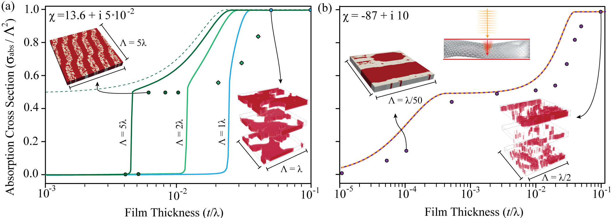
Figure 4: Absorption cross section bounds for a planewave incident on a periodic film. Absorption cross section bounds for any periodic structure (e.g. grating, metasurface) of period $\Lambda$ and electric susceptibility (a) $\chi=13.6+i~{}5\cdot 10^{-2}$ (silicon at $0.8\mu m$) and (b) $\chi=-87+i~{}10$ (gold at $1.5\mu m$) that can be contained within a planar boundary of thickness $t/\lambda$. Dots correspond to actual absorption cross section values discovered using inverse design following the algorithm described in Ref. Jin et al. [2020]. A number of visualizations of the associated structures, along with a schematic of the absorption process investigated, are included as insets. All discovered designs with $t/\lambda<10^{-2}$ consist of a single layer, uniform in the normal direction. For larger thickness, optimization of three equally thick uniform layers is needed to achieve the reported absorption cross sections (eventually reaching absorption saturation). Like prior figures, solid lines are found by solving (LABEL:optProb) under the constraint that total power is conserved, while dashed lines, coinciding with the solid line in (b), are found by only imposing the constraint of real power conservation. As shown in (a), total power conservation bounds for dielectric media depend on the square period supposed. Moving from left to right, the periods used in the inverse design optimizations are $\Lambda=\left\{5\lambda,~{}5\lambda,~{}5\lambda,~{}5\lambda,~{}4\lambda,~{}2\lambda,~{}3\lambda/2,~{}3\lambda/2,~{}\lambda,~{}\lambda\right\}$. Results for metals ($\operatorname{Re}\left[\chi\right]<0$) do not depend on the periodicity of the system. Discussion of additional bound features relating solely to imposing the conservation of real can be found in Ref. Molesky et al. [2019] and Ref. Kuang et al. [2020].

For both spherically bounded examples, the distribution of the power density within the domain between different angular momentum numbers is strongly tethered to the radius of the boundary. Specifically, the coefficients of the electric field, for a unit normalized electric field amplitude, in terms of the regular (finite at the origin) $\textbf{RM}_{\ell,m}$ and $\textbf{RN}_{\ell,m}$ solutions of Maxwell’s equations in spherical coordinates, (28), are

$$\hat{\textbf{E}}_{i}=\sum_{\ell=1}^{\infty}\sum_{\pm} i^{\ell+1}\sqrt{(2\ell+1)\pi}~{}\textbf{RM}_{\ell,\pm 1}\left(r,\theta,\phi\right)\pm$$

$$i^{\ell+1}\sqrt{\left(2\ell+1\right)\pi}~{}\textbf{RN}_{\ell,\pm 1}\left(r,\theta,\phi\right),$$ (34)

with $r$ standing for the wave vector normalized radius (the product of the true radius and $k=2\pi/\lambda$). Through $\operatorname{Asym}\left[\mathbb{U}\right]$ (34) establishes a link between the magnitude of the radiative efficacy of each channel Molesky et al. [2020], or $\ell$ number, and its potential for enhancing scattering cross sections: if the planewave expansion coefficient of a given channel is large, then so is $\operatorname{Asym}\left[\mathbb{G}^{\text{0}}_{\ell}\right]$, tightening the constraint that real power must be conserved. This leads to a complementary action of the power constraints. For any given combination of material and radius, save $\operatorname{Re}\left[\chi\right]=-3$ in the $R\rightarrow 0$ limit, either real or reactive power conservation limits induced polarization currents in the medium more severely than what would be expected based solely on the material loss figure of merit

$$\zeta_{\text{mat}}=\frac{\left|\chi\right|^{2}}{\operatorname{Im}\left[\chi\right]},$$ (35)

widely considered in past work on electromagnetic bounds for arbitrary materials and structures Miller et al. [2016], Yang et al. [2017, 2018], Molesky et al. [2020]. (An explanation of the origin and usefulness of this quantity is given in Sec. II.) In Fig. 2 and Fig. 3, dashed curves depict cross section limits attained when only the conservation of real power, (15), is imposed, as in Ref. Kuang et al. [2020], and solid curves result when reactive power conservation is additionally included. All results are found using the Lagrange duality approach described in Sec. I and are strongly dual Boyd and Vandenberghe [2004].

Conversely, the example bounds for periodic films shown in Fig. 4 are strongly dual only when absorption is near zero. Outside this regime, and the associated sharp transition to resonant response, all major features, including the half absorption plateaus, are seen to be accounted for by the conservation of real power, and are thus described by the growth of the radiative efficacies (singular values of $\operatorname{Asym}\left[\mathbb{G}^{\text{0}}\right]$) of the two channels with zero in-plane wave vector Molesky et al. [2019], Kuang et al. [2020].

Quasi-Static Regime ($R/\lambda\rightarrow 0,~{}t/\lambda\rightarrow 0$) Recalling the conclusions of Sec. III B., the simultaneous conservation of real and reactive power has far-reaching implications for electromagnetic power transfer when all dimensions of the confining domain are small. The analog of the optical theorem for reactive power, (14), adds phase information on top of the maximum polarization magnitude set by the conservation of real power, (15); and so, when both constraints are taken into account, (LABEL:optProb) captures the fact it is not always possible to produce a resonant structure given any single material, of electric susceptibility $\chi$, and a maximal characteristic size, $R$. In fact, there are rather strict requirements that must be met for resonant response to be achievable. Crucially, it must be possible to effectively confine the scattered electromagnetic field, resulting from the polarization currents created in the structure by the incident (source) wave, within the spherical volume. As validated by the cross section bounds of Fig. 2 and Fig. 3, the only mechanism by which such confinement can be achieved while also allowing interactions with propagating waves as $R/\lambda\rightarrow 0$, is the excitation of localized plasmon-polaritons, occurring for $\operatorname{Re}\left[\chi\right]=-3$ if the domain is completely filled with material Novotny and Hecht [2012].

If $\operatorname{Re}\left[\chi\right]$ is larger than this value, excluding small deviations that appear for weak metals between $-2\gtrsim\operatorname{Re}\left[\chi\right]\geq-3$, then, as confirmed by the tiny achievable cross section values, resonant response with a propagating wave is not possible. Therefore, the largest allowed power transfer happens when the material simply fills the entire domain, and as such, maximal scattering cross sections exhibit the same susceptibility dependence encountered in Rayleigh scattering Tsang et al. [2004]. Applying (33), the maximal magnitude of the interaction that can occur in a dielectric structure between the (normalized) incident field and the polarization current it excites is

$$\zeta_{\text{Ray}}=\frac{1}{\sqrt{\left(\frac{1}{3}+\frac{\operatorname{Re}\left[\chi\right]}{\left|\chi\right|^{2}}\right)^{2}+\left(\rho^{{}_{\mathbb{G}\textbf{N}}}_{1}+\frac{\operatorname{Im}\left[\chi\right]}{\left|\chi\right|^{2}}\right)^{2}}} \left(\operatorname{Re}\left[\chi\right]\geq 0\right).$$ (36)

with

$$\rho^{{}_{\mathbb{G}\textbf{N}}}_{1}=\frac{2}{9}\left(\frac{2\pi R}{\lambda}\right)^{3}$$ (37)

denoting the radiative efficacy of the $\ell=1,~{}m=\pm 1,~{}0$ N polarized channel. Employing the power forms given in Sec. I, the scattering cross section of any structure, under the above assumptions, must obey the relations

$$\frac{\sigma_{\text{sca}}}{\sigma_{\text{geo}}}\leq\frac{3}{2}\frac{(\rho^{{}_{\mathbb{G}\textbf{N}}}_{1})^{2}}{\left(\frac{1}{3}+\frac{\operatorname{Re}\left[\chi\right]}{\left|\chi\right|^{2}}\right)^{2}+\left(\rho^{{}_{\mathbb{G}\textbf{N}}}_{1}+\frac{\operatorname{Im}\left[\chi\right]}{\left|\chi\right|^{2}}\right)^{2}}\left(\frac{\lambda}{2\pi R}\right)^{2}$$

$$\frac{\sigma_{\text{abs}}}{\sigma_{\text{geo}}}\leq\frac{3}{2}\frac{\rho^{{}_{\mathbb{G}\textbf{N}}}_{1}\left(\operatorname{Im}\left[\chi\right]/\left|\chi\right|^{2}\right)}{\left(\frac{1}{3}+\frac{\operatorname{Re}\left[\chi\right]}{\left|\chi\right|^{2}}\right)^{2}+\left(\rho^{{}_{\mathbb{G}\textbf{N}}}_{1}+\frac{\operatorname{Im}\left[\chi\right]}{\left|\chi\right|^{2}}\right)^{2}}\left(\frac{\lambda}{2\pi R}\right)^{2}.$$ (38)

In stark contrast to $\zeta_{\text{mat}}$, $\zeta_{\text{Ray}}$ decreases for increasing $\operatorname{Re}\left[\chi\right]$ and has a negligible dependence on material absorption, $\operatorname{Im}\left[\chi\right]$. Comparing the dashed and full lines of Fig. 2 and Fig. 3, particularly Fig. 2 (b) and Fig. 3 (b), the resonance gap between these two forms can be quite extreme for realistic dielectrics. For example, $\zeta_{\text{mat}}\approx 10^{7}$ for silicon at $\lambda=1.5\mu\mathrm{m}$, with $\chi\approx 11+i~{}10^{-5}$  Palik [1998].

As $\operatorname{Re}\left[\chi\right]$ shifts to increasingly negative values, geometries supporting localized plasmon–polariton resonances become possible, and past $\operatorname{Re}\left[\chi\right]=-3$ cross section limits display resonant response characteristics. The power exchange between the incident field and the generated polarization currents is then, asymptotically, restricted to be smaller than the “diluted” material figure of merit

$$\zeta_{\text{dil}}=\frac{\left|\chi\right|}{\operatorname{Re}\left[\chi\right]}\frac{1}{\rho^{{}_{\mathbb{G}\textbf{N}}}_{1}+\frac{\operatorname{Im}\left[\chi\right]}{\left|3\operatorname{Re}\left[\chi\right]\right|}} \left(\operatorname{Re}\left[\chi\right]\leq-3\right),$$ (39)

leading to cross section limits of

$$\frac{\sigma_{\text{sca}}}{\sigma_{\text{geo}}}\leq\frac{3}{2} \left(\frac{\left|\chi\right|}{\left|\operatorname{Re}\left[\chi\right]\right|}\right)^{2}\frac{(\rho^{{}_{\mathbb{G}\textbf{N}}}_{1})^{2}}{\left(\rho^{{}_{\mathbb{G}\textbf{N}}}_{1}+\operatorname{Im}\left[\chi\right]/\left|3\operatorname{Re}\left[\chi\right]\right|\right)^{2}}\left(\frac{\lambda}{2\pi R}\right)^{2}$$

$$\frac{\sigma_{\text{abs}}}{\sigma_{\text{geo}}}\leq\frac{3}{2} \frac{\left|\chi\right|}{\left|\operatorname{Re}\left[\chi\right]\right|}\Bigg{(}\frac{\rho^{{}_{\mathbb{G}\textbf{N}}}_{1}\left(\operatorname{Im}\left[\chi\right]/\left|3\operatorname{Re}\left[\chi\right]\right|\right)}{\left(\rho^{{}_{\mathbb{G}\textbf{N}}}_{1}+\operatorname{Im}\left[\chi\right]/\left|3\operatorname{Re}\left[\chi\right]\right|\right)^{2}}$$

$$-\frac{(\rho^{{}_{\mathbb{G}\textbf{N}}}_{1})^{2}\left(\left|\chi\right|/\left|\operatorname{Re}\left[\chi\right]\right|-1\right)}{\left(\rho^{{}_{\mathbb{G}\textbf{N}}}_{1}+\operatorname{Im}\left[\chi\right]/\left|3\operatorname{Re}\left[\chi\right]\right|\right)^{2}}\Bigg{)}\left(\frac{\lambda}{2\pi R}\right)^{2}.$$ (40)

The “dilution” modifier is chosen as the form of (39), disregarding the radiative efficacy $\rho^{{}_{\mathbb{G}\textbf{N}}}_{1}$, is equivalent to the material loss figure of merit $\zeta_{\text{mat}}$ if a “dilution factor” is introduced to shift $\operatorname{Re}\left[\chi\right]$ to $-3$. That is, considering the low-loss limit $\operatorname{Im}\left[\chi\right]\ll\left|\chi\right|$, if it is supposed that the magnitude of $\operatorname{Re}\left[\chi\right]$ is rescaled to match the localized resonance condition of a spherical nanoparticle, then $\zeta_{\text{mat}}\rightarrow 3\left|\chi\right|/\operatorname{Im}\left[\chi\right]$, which is equal to the expression for $\zeta_{\text{dil}}$ in the limit $\rho^{{}_{\mathbb{G}\textbf{N}}}_{1}\rightarrow 0$. (Due to its connection with the localized plasmon resonance of a spherical nanoparticle, the ratio $\left|\chi\right|/\operatorname{Im}\left[\chi\right]$ is commonly encountered in discussing the potential of different material options for plasmonic applications Maier [2007], West et al. [2010].)

The validity of (39) internally rests on the assumption that the wavelength is much larger than any structural feature. Since this is also the central criterion for most homogenization descriptions of electromagnetic response to be applicable Markel [2016], it is sensible that material structuring limited to tiny domains can, at best, alter effective medium parameters Liu et al. [2007], Cai and Shalaev [2010], Jahani and Jacob [2016]. Equation (39) proves that the implications of this picture are universally valid for both scattering and absorption in strong metals. However, many commonly stated effective medium models also predict that there are structures capable of creating effective susceptibility responses more negative than either of the constituent materials Simovski [2010], Choy [2015], Mackay and Lakhtakia [2015], Petersen et al. [2016], Lei et al. [2017]. For example, the Maxwell–Garnett formula for mono-dispersed spherical vacuum inclusions in a background host is

$$\chi_{\text{eff}}=\left(1+\chi_{\text{h}}\right)\frac{1-2f\chi_{h}/\left(3+2\chi_{h}\right)}{1+f\chi_{h}/\left(3+2\chi_{h}\right)}-1,$$ (41)

where $f$ is the volume filling fraction of the inclusions and $\chi_{\text{h}}$ is electric susceptibility of the host Merrill et al. [1999]. Based on (41), using the iterative argument given in Ref. Merrill et al. [1999], it should be anticipated that low-loss resonant response would be achievable shortly after $\operatorname{Re}\left[\chi\right]$ drops below $-1$. While cross sections do begin to grow before $\operatorname{Re}\left[\chi\right]=-3$, it is clear that this Maxwell-Garnett condition is not sufficient. Dilution via (41) also yields a different dependence on material loss-values than that predicted by (39), with (41) consistently giving slightly larger effective losses.

It is also interesting to compare (38) and (40) with coupled mode descriptions of scattering phenomena in the single channel limit Hamam et al. [2007],

$$\frac{\sigma_{\text{sca}}}{\sigma_{\text{geo}}} =~{}6~{}\frac{\gamma_{\text{rad}}^{2}}{\left(\omega-\omega_{\text{res}}\right)^{2}+\left(\gamma_{\text{rad}}+\gamma_{\text{abs}}\right)^{2}}\left(\frac{\lambda}{2\pi R}\right)^{2}$$

$$\frac{\sigma_{\text{abs}}}{\sigma_{\text{geo}}} =~{}6~{}\frac{\gamma_{\text{rad}}\gamma_{\text{abs}}}{\left(\omega-\omega_{\text{res}}\right)^{2}+\left(\gamma_{\text{rad}}+\gamma_{\text{abs}}\right)^{2}}\left(\frac{\lambda}{2\pi R}\right)^{2},$$ (42)

where $\gamma_{\text{rad}}$ and $\gamma_{\text{abs}}$ are the geometry-specific radiative and absorptive decay rates associated with a given resonant mode of frequency $\omega_{\text{res}}$. Up to a missing factor of $4$, which is accounted for by the facts that (38) and (40) represent maximum quantities Kwon and Pozar [2009], Liberal et al. [2014b] and that scattering cannot occur without absorption Miller et al. [2016], there is a clear symmetry of form between (38) and (40) and (42), provided $\operatorname{Im}\left[\chi\right]\ll\left|\operatorname{Re}\left[\chi\right]\right|$ (as coupled mode theory requires the assumption of low loss). The two sets of expressions agree under the substitutions

$$\gamma_{\text{abs}}\rightarrow\operatorname{Im}\left[\chi\right]/\left|\chi\right|^{2}$$

$$\left(\omega-\omega_{\text{res}}\right)^{2}\rightarrow\left(1/3+\operatorname{Re}\left[\chi\right]/\left|\chi\right|^{2}\right)^{2},$$

when the system is off resonance, and

$$\gamma_{\text{abs}}\rightarrow\operatorname{Im}\left[\chi\right]/\left|3\operatorname{Re}\left[\chi\right]\right|,$$

when the system is on resonance; in both situations, $\gamma_{\text{rad}}\rightarrow\rho^{{}_{\mathbb{G}\textbf{N}}}_{1}$. Since (38) and (40) are bounds, and not descriptions of any particular mode, these associations may be understood as “best case” parameters for what could be achieved in any geometry supporting a single mode, and are thus closely linked to prior limits based on coupled mode theory Hamam et al. [2007], Verslegers et al. [2010], Yu et al. [2010b, a], Yu and Fan [2011], Ruan and Fan [2012]. Notably, the comparison precludes any resonant geometry from achieving the rate-matching condition of $\gamma_{\text{rad}}=\gamma_{\text{abs}}$ if it is confined to a small ball. Precisely, the only candidate materials are fictitious metals with $-3\gtrsim\operatorname{Re}\left[\chi\right]$ and $\operatorname{Im}\left[\chi\right]\rightarrow 0$, since the radiative efficacy $\rho^{{}_{\mathbb{G}\textbf{N}}}_{1}\rightarrow 0$ with vanishing object size.

This situation, a fictitiously low loss metallic nanoparticle, is also the most relevant condition under which the bounds asymptotically reach arbitrarily large values. However, as we have discussed in Ref. Molesky et al. [2019] in the context of angle-integrated planewave absorption, unbounded growth requires saturation of an unbounded number of angular momentum $\ell$ indices (radiation channels). For any particular $\ell$, saturation is approximately achieved as $R\rightarrow 0$ when $\rho_{\ell}^{{}_{\mathbb{G}\textbf{N}}},~{}\rho_{\ell}^{{}_{\mathbb{G}\textbf{M}}}\gtrsim\operatorname{Im}\left[\chi\right]/\left|3\operatorname{Re}\left[\chi\right]\right|$. Therefore, the relation between the radiative efficacies and the angular momentum number $\ell$, with

$$\rho^{{}_{\mathbb{G}\textbf{N}}}_{\ell}\left(R\right)= \frac{\pi\left(kR\right)^{2}}{4}$$

$$\Bigg{[}\frac{\ell+1}{2\ell+1}\left(J_{\ell-\frac{1}{2}}^{2}\left(kR\right)-J_{\ell+\frac{1}{2}}\left(kR\right)J_{\ell-\frac{3}{2}}\left(kR\right)\right)$$

$$+\frac{\ell}{2\ell+1}\left(J_{\ell+\frac{3}{2}}^{2}\left(kR\right)-J_{\ell+\frac{1}{2}}\left(kR\right)J_{\ell+\frac{5}{2}}\left(kR\right)\right)\Bigg{]},$$

$$\rho^{{}_{\mathbb{G}\textbf{M}}}_{\ell}\left(R\right)= \frac{\pi\left(kR\right)^{2}}{4}\left(J_{\ell+\frac{1}{2}}^{2}\left(kR\right)-J_{\ell-\frac{1}{2}}\left(kR\right)J_{\ell+\frac{3}{2}}\left(kR\right)\right),$$ (43)

imparted through the cylindrical Bessel functions, with

$$J_{\ell+p}\left(kR\right)<\frac{1}{\Gamma\left(\ell+p+1\right)}\left(\frac{kR}{2}\right)^{\ell+p}$$ (44)

for $kR<\sqrt{8\Gamma\left(\ell+p+3\right)}$, implies that so long as real power is conserved, bounds on cross section enhancement exhibit sublogarithmic growth with vanishing material loss, $\operatorname{Im}\left[\chi\right]\rightarrow 0$. (Proof of this statement, in all important regards, follows from the derivation given in Ref. Molesky et al. [2019]. The stated inequality follows from the power series of the cylindrical Bessel functions DLMF .) As seen in the supporting figures, Fig. 2 and Fig. 3, in practice this scaling behavior is of little consequence.

For periodic films (e.g., gratings, photonic crystals, and metasurfaces), the central feature of (LABEL:optProb) absent from the models of Ref. Molesky et al. [2019] and Ref. Kuang et al. [2020] is the initial suppression and sharp onset of resonant absorption for thin dielectrics. The above findings for compact domains, and practical experience, both suggest that the existence of such a critical thickness (depending of the magnitude of $\operatorname{Re}\left[\chi\right]$) for dielectric materials is reasonable. However, the dependence of this thickness threshold on the period of the system, physically associated with the presence of leaky-mode resonances Joannopoulos et al. [2008], is perhaps less expected. The origin of the relation traces to the properties of $\mathbb{G}^{\text{0}}$ for an extended (infinite) system. Crossing over the light line boundary between propagating and evanescent waves, there are vectors within the basis described in Sec. VII, $\left|\textbf{X}\right>=\left|\hat{\textbf{RX}}^{\left(-\right)}\left(\text{k}_{p}\right)\right>$, that allow $\left<\textbf{X}\right|\operatorname{Sym}\left[\mathbb{G}^{\text{0}}\right]\left|\textbf{X}\right>$ to be arbitrarily negative and $\left<\textbf{X}\right|\operatorname{Asym}\left[\mathbb{G}^{\text{0}}\right]\left|\textbf{X}\right>=0$. These characteristics allow reactive power conservation, (14), to be trivially satisfied for any possible polarization current. However, when a finite period is imposed on the system, modes arbitrarily near the light line are not allowed, and in turn, the necessity of conserving reactive power may imply that resonant response is not possible for particular values of $t$ and $\chi$. As exemplified in Fig. 4, knowledge of the critical thickness at which such leaky modes can be supported for a given period and material may be of substantial benefit to the design of large scale metasurfaces Wu et al. [2019], Lin et al. [2019], Jin et al. [2020].

Wavelength Scale Regime ($R/\lambda\gtrsim 0.1,~{}t/\lambda\gtrsim 0.01$) For boundary radii approaching wavelength size, the applicability of the quasi-static results for spherical confining region quoted under the previous subheading becomes increasingly tenuous. The growth of planewave amplitude coefficients into angular momentum numbers (channels) beyond $\ell=1$ opens the possibility of utilizing a wider range of wave physics (e.g., leaky and guided resonances Li et al. [2019], Lee and Magnusson [2019]), and correspondingly, reactive power conservation (resonance creation) becomes a weaker requirement.

These factors lead to a more intricate interplay between the two power constraints, causing the sharp jumps observed for dielectrics in Fig. 2 and Fig. 3, which manifest, mechanically, in rapid changes to the properties of the scattering $\mathbb{T}$ operator constraint relations, especially (14) applied to dielectric materials. The behavior is first observed in the $\ell=1$ channel, with the initial peaks in Fig. 2(b) and Fig. 3(b) following closely after the half wavelength condition

$$\left(\text{min}~{}r\right)~{}\ni~{}\partial j_{1}\left(\sqrt{\operatorname{Re}\left[\chi\right]}~{}\frac{2\pi r}{\lambda}\right)/\partial r=0,$$

and the second peaks occurring near the full wavelength condition,

$$\left(\text{min}~{}r\right)~{}\ni~{}j_{1}\left(\sqrt{\operatorname{Re}\left[\chi\right]}~{}\frac{2\pi r}{\lambda}\right)=0.$$

This second criterion is also the approximate resonance location for a homogeneous dielectric sphere of index $\sqrt{\chi}$  Newton [2013], the spherical analogs of the Fabry–Perot condition Yariv and Yeh [2006], making its appearance consistent with the Rayleigh response predictions of (36). At the same time, as previously remarked, the inflation of the boundary also increases the radiative efficacy of each channel as described by (43) (further discussed in Ref.  Molesky et al. [2019] and Sec. II). Via the connection of $\operatorname{Asym}\left[\mathbb{U}_{\ell}\right]$ to $\operatorname{Asym}\left[\mathbb{G}^{\text{0}}_{\ell}\right]$, (13), this causes the conservation of real power to become a more restrictive constraint for generating strong polarization currents throughout the volume available to structuring. (That is, maintaining the ratio of $\operatorname{Im}\left[\left<\textbf{S}^{(1)}|\textbf{T}\right>\right]$ and $\left<\textbf{T}\right|\operatorname{Asym}\left[\mathbb{U}\right]\left|\textbf{T}\right>$ becomes increasingly restrictive, while maintaining the ratio of $\operatorname{Re}\left[\left<\textbf{S}^{(1)}|\textbf{T}\right>\right]$ and $\left<\textbf{T}\right|\operatorname{Sym}\left[\mathbb{U}\right]\left|\textbf{T}\right>$ becomes increasingly simple.) Subsequently, rather than completely releasing to an enhancement value approaching $\zeta_{\text{mat}}$, the bound slips and catches.

For periodic films, all features seen at both wavelength and ray optic thickness scales are fully accounted for by the conservation of real power and the associated radiative efficacies of $\operatorname{Asym}\left[\mathbb{G}^{\text{0}}\right]$ at normal incidence. Detailed discussions of these quantities are given in Ref. Molesky et al. [2019] and Ref. Kuang et al. [2020]. The most interesting result, that the bounds plateau for film thickness between roughly $t/\lambda=10^{-4}$ and $t/\lambda=10^{-2}$, is caused by the fact that at these thicknesses only a single symmetric mode is bright. Accordingly, the power radiated to the far-field by the excited polarization current can not be canceled, and only half of the total power of the incident wave can be extracted through absorption Molesky et al. [2019].

Ray Optics Regime ($R/\lambda\gg 1,~{}t/\lambda\gg 10^{-1}$) In the large boundary limit, achievable scattering interactions in any given channel are increasingly dominated by the conservation of real power through the growth of radiative losses. Correspondingly, the dash bounds, calculated by asserting only that the sum of the scattered and absorbed power must not exceed the power drawn from the incident beam, coincide with those arising from total power conservation to increasingly good accuracy. Making this reduction, limits for either cross section enhancement quantity become largely congruous to the angle-integrated absorption bounds given in Ref. Molesky et al. [2019]. The planewave expansion coefficients of (34) exhibit exactly the same per-channel characteristics considered in that article, and so, the same asymptotic behavior is encountered. Regardless of the selected susceptibility $\chi$, for a sufficiently large radius, each of the power objectives described in Sec. I begins to scale as the geometric cross section of the bounding sphere. For absorption, this leads to a value equal to the geometric cross section of the confining ball, $\pi R^{2}$. For extinction and scattering, a value of $4\pi R^{2}$ is found, two times larger than what would be expected based on the extinction paradox Żakowicz [2002], Berg et al. [2011]. The genesis of this additional factor is presently unknown, and investigation of the properties of the optimal polarization current of these curious results merits further study.

V Summary Remarks

The ability of metals and polaritonic materials to confine light in subwavelength volumes without the need for any other surrounding structure (plasmon–polaritons Williams et al. [2008], Neutens et al. [2009]), coupled with the variety of geometric wave effects achievable in dielectric media (band gaps Foresi et al. [1997], Chen et al. [2016], index guiding Li et al. [2017b], le20163d, topological states Ozawa et al. [2019], Khanikaev and Shvets [2017]), rest as the bedrock of contemporary photonic design. Yet, the relative abilities of these two overarching approaches for controlling light–matter interactions remains a widely studied topic Noginov and Khurgin [2018], Khurgin [2018], Ballarini and De Liberato [2019]. The broad strokes are well established. The possibility of subwavelength confinement and large field enhancements offered by metals is offset by the fact these effects are fundamentally linked to substantial material loss Khurgin [2018]. Through interference, dielectric architectures may also confine and intensify electromagnetic fields, and can do so without large accompanying material absorption Lin et al. [2016a]; but, accessing this potential invariably requires larger domains and more complex structures. While comparisons within rigidly defined subclasses have been made Liu et al. [2016], the merit of a particular method for a particular design challenge is almost always an open question. As with the rising need for limits in computational approaches highlighted in the introduction, a central driver of debate is the lack of concrete (pertinent) knowledge of what is possible, beyond qualitative arguments.

We believe that the simple instructive cross section examples shown in Sec. IV are compelling evidence that the generation of bounds based on constraints derived from the $\mathbb{T}$ operator and Lagrange duality offers a path towards progress; and that by translating this method beyond the spectral basis employed here, onto a completely geometry agnostic numerical algorithm, it will be possible to analyze the relative trade offs associated with various kinds of optical devices. Through bound calculations varying material and domain parameters, the significance of different design elements from the perspective of device performance should be ascertainable in a number of technologically relevant areas. The basic scattering interaction quantities given in Sec. I lie at the core of engineering the radiative efficacy of quantum emitters Lu et al. [2017], Davoyan and Atwater [2018], Crook et al. [2020], resonant response of cavities Lin et al. [2016b], Liu and Houck [2017], Wang et al. [2018], design characteristics of metasurfaces Kruk and Kivshar [2017], Groever et al. [2017], Lewi et al. [2019], and the efficacy of light trapping Yu et al. [2010a], Sheng et al. [2012] devices and luminescent Zalogina et al. [2018], Valenta et al. [2019] and fluorescent Li et al. [2017a], Simovski [2019] sources. They are also central building blocks of quantum and nonlinear phenomena like Förster energy transfer Cortes and Jacob [2018], Raman scattering Michon et al. [2019], and frequency conversion Lin et al. [2016a].

As seen in Sec. IV, relations (14) and (15) are amenable to numerical evaluation under realistic photonic settings (for practical domain sizes and materials) and sufficiently broad to provide both quantitative guidance and physical insights: as the size of an object interacting with a planewave grows, there is a transition from the volumetric (or super volumetric) scaling characteristic of subwavelength objects to the geometric cross section dependence characteristic of ray optics; critical sizes exist below which it is impossible to create dielectric resonances; material loss dictates achievable interactions strengths only once it becomes feasible to achieve resonant response and significant coupling to the incident field.

Several generalizations of the formalism should be possible. First, there is an apparent synergy with the work of Angeris, Vučković and Boyd Angeris et al. [2019] for inverse design applications. The optimal vectors found using (LABEL:optProb) provide intuitive target fields. Second, following the arguments given in the work of Shim el al. Shim et al. [2019] it would seem that (LABEL:optProb) can be further enlarged to include finite bandwidth dispersion information, accounting for the full analytic features of the electric susceptibility $\chi\left(\omega\right)$. Finally, by combining the respective strengths of both classes of materials, hybrid metal-dielectric structures offer the potential of realizing more performant devices. The generalization of (LABEL:optProb) to incorporate multiple material regions (multi-region scattering Molesky et al. [2020]) as an aid to these efforts stands as an important direction of ongoing study. As we have stated earlier, as the method relies only on scattering theory, almost all lines of reasoning we have presented apply equally to acoustics, quantum mechanics, and other wave physics.

VI Acknowledgments

This work was supported by the National Science Foundation under Grants No. DMR-1454836, DMR 1420541, DGE 1148900, the Cornell Center for Materials Research MRSEC (award no. DMR1719875), and the Defense Advanced Research Projects Agency (DARPA) under Agreement No. HR00112090011. The views, opinions and/or findings expressed herein are those of the authors and should not be interpreted as representing the official views or policies of any institution. We thank Prashanth S. Venkataram, Jason Necaise, and Prof. Shanhui Fan for useful comments.

VII Appendix

VII.1 Numerical Stability of the Arnoldi Processes

With perfect numerical accuracy, the convergence of $\mathbb{A}_{\ell}$ is guaranteed in a finite number of iterations. The strictly diagonal elements of each $\mathbb{U}_{\ell}$ matrix, $\mathbb{V}^{\dagger-1}_{\ell}$ , remain constant while the off diagonal coupling coefficients introduced by $\operatorname{Sym}\left[\mathbb{G}^{\text{0}\dagger}_{\ell}\right]$ gradually decay with every iterations. Thus, at a certain point, the diagonal $\mathbb{V}^{\dagger-1}_{\ell}$ entries eventually overwhelm all other contributions, terminating the $\mathbb{U}_{\ell}$ matrix. (As the magnitude of the susceptibility considered increases, $\mathbb{V}^{\dagger-1}$ shrinks and more Arnoldi iterations are required.)

Still, there are pitfalls that must be avoided when numerically implementing an Arnoldi iteration, caused by the singularity of the outgoing N waves at the origin. The issue is illustrated by considering the image of RN under $\mathbb{G}^{\text{0}}$ (26), with

$$\textbf{N}_{\ell,m}\left(\textbf{x}\right)=\frac{\sqrt{\ell\left(\ell+1\right)}}{r}\text{h}_{\ell}^{\left(1\right)}\left(r\right)\text{A}_{\ell,m}^{\left(3\right)}+\frac{\partial\left(x~{}\text{h}_{\ell}^{\left(1\right)}\left(\text{r}\right)\right)}{r}\text{A}_{\ell,m}^{\left(2\right)},$$ (45)

using the normalized vector spherical harmonics as described in Ref Kristensson [2016]. Near the origin, $r\rightarrow 0$, the leading order radial dependencies of (28) and (45) are

$$\textbf{RN}_{\ell,m}= \left(\frac{\ell+1}{(2\ell+1)!!}\left(r\right)^{\ell-1}+\mathcal{O}\left(r^{\ell+1}\right)\right)\text{A}_{\ell,m}^{\left(2\right)}+$$

$$\left(\frac{\sqrt{\ell(\ell+1)}}{(2\ell+1)!!}r^{\ell-1}+\mathcal{O}\left(r^{\ell+1}\right)\right)\text{A}_{\ell,m}^{\left(3\right)},$$ (46)

$$\textbf{N}_{\ell,m}= \left(\frac{i\ell(2\ell-1)!!}{r^{\ell+2}}+\mathcal{O}\left(r^{-\ell}\right)\right)\text{A}^{\left(2\right)}_{\ell,m}+$$

$$\left(\frac{-i(2\ell-1)!!\sqrt{\ell(\ell+1)}}{r^{\ell+2}}+\mathcal{O}\left(r^{-\ell}\right)\right)\text{A}_{\ell,m}^{\left(3\right)}.$$ (47)

From (26), the image of $\textbf{RN}_{\ell,m}$ under the Green function restricted to a spherical domain with radius $R$ is

$$\mathbb{G}^{\text{0}}\textbf{RN}=\textbf{RN}(\textbf{r})\textbf{RN}_{co}(\textbf{r})+\textbf{N}(\textbf{r})\textbf{N}_{co}(\textbf{r})-\textbf{RN}(\textbf{r})~{}\textbf{A}^{\left(3\right)}_{\ell,m}$$ (48)

where the final term is the $\delta$-function contribution, and the $\textbf{RN}_{co}(\textbf{r})$ and $\textbf{N}_{co}(\textbf{r})$ terms are given by

$$\textbf{N}_{co}(\textbf{r}) =i\iint_{\Omega^{\prime}}\int_{0}^{r}r^{\prime 2}\textbf{RN}(\textbf{r'})\textbf{RN}(\textbf{r'})\text{d}r^{\prime}\text{d}\Omega^{\prime},$$

$$\textbf{RN}_{co}(\textbf{r}) =i\iint_{\Omega^{\prime}}\int_{r}^{R}r^{\prime 2}\textbf{N}(\textbf{r'})\textbf{RN}(\textbf{r'})\text{d}r^{\prime}\text{d}\Omega^{\prime}.$$ (49)

Exploiting the orthogonality of the vector spherical harmonics, the leading radial order for $\textbf{N}_{co}(\textbf{r})$ is $r^{2\ell+1}$. Therefore, the $\textbf{N}(\textbf{r})\textbf{N}_{co}(\textbf{r})$ term has a leading radial order of $r^{\ell-1}$, the same as the starting vector $\textbf{RN}(\textbf{r})$. At first sight, $\textbf{RN}_{co}(\textbf{r})$ is more troubling. The dominate radial orders are $r^{\prime-\ell}$ for $r^{\prime 2}\textbf{N}(\textbf{r'})$ and $r^{\prime\ell-1}$ for $\textbf{RN}(\textbf{r'})$. Thus, it would seem that the integrand has an $r^{\prime-1}$ dependence, which would result in a logarithmic divergence at the origin. A more careful consideration, however, shows that the leading order terms from $\textbf{A}^{\left(2\right)}_{\ell,m}$ and $\textbf{A}^{\left(3\right)}_{\ell,m}$ cancel as

$$\textbf{RN}_{co}(\textbf{r})= ~{}i\iint_{\Omega^{\prime}}\bigg{(}\frac{i\ell(\ell+1)}{2\ell+1}r^{\prime-1}\text{A}^{\left(2\right)}_{\ell,m}\cdot\text{A}^{\left(2\right)}_{\ell,m}-$$

$$\frac{i\ell(\ell+1)}{2\ell+1}r^{\prime-1}\text{A}^{\left(3\right)}_{\ell,m}\cdot\text{A}^{\left(3\right)}_{\ell,m}+\mathcal{O}\left(r^{\prime}\right)\text{d}r^{\prime}\bigg{)}\text{d}\Omega$$

$$= ~{}\mathcal{O}\left(r^{2}\right).$$ (50)

The key to this cancellation is the ratio of the $\text{A}_{\ell,m}^{\left(2\right)}$ and $\text{A}^{\left(3\right)}_{\ell,m}$ terms, $\sqrt{(\ell+1)/\ell}$. So long as this ratio is maintained, the $\textbf{RN}_{co}$ factor does not generate logarithmic contributions, and in turn this causes the leading order ratio to remain intact under the further action of $\mathbb{G}^{\text{0}}$. By insuring that this does in fact occur, the Arnoldi process may continue to stably iterate until convergence is achieved. Consider any vector

$$\textbf{P}=p\left(r^{\ell-1}\text{A}_{\ell,m}^{\left(2\right)}+\sqrt{\frac{\ell}{\ell+1}}r^{\ell-1}\text{A}_{\ell,m}^{\left(3\right)}\right),$$ (51)

where $p$ is a constant. ($\textbf{RN}_{\ell,m}$ are vectors of this form.) The image under of this vector under $\mathbb{G}^{\text{0}}$ is

$$\mathbb{G}^{\text{0}}\textbf{P}= ~{}\textbf{RN}_{\ell,m}\left(\textbf{r}\right)\textbf{RN}^{{}_{\textbf{P}}}_{co}\left(\textbf{r}\right)+\textbf{N}_{\ell,m}\left(\textbf{r}\right)\textbf{N}^{{}_{\textbf{P}}}_{co}(\textbf{r})-$$

$$p~{}\sqrt{\frac{\ell}{\ell+1}}r^{\ell-1}\text{A}^{\left(3\right)}_{\ell,m},$$ (52)

with

$$\textbf{RN}^{{}_{\textbf{P}}}_{co}(\textbf{r})= ~{}p\int_{r}^{R}\Big{(}\frac{i\ell\left(2\ell-1\right)!!}{r^{\prime\ell}}r^{\prime\ell-1}-$$

$$\frac{i\ell\left(2\ell-1\right)!!}{r^{\prime\ell}}r^{\prime\ell-1}+\mathcal{O}\left(r^{\prime}\right)\Big{)}\text{d}r^{\prime}$$

$$= ~{}C\left(R\right)+\mathcal{O}\left(r^{2}\right),$$ (53)

$C\left(R\right)$ a constant of $r$ coming from the fixed upper integration limit $R$, and

$$\textbf{N}^{{}_{\textbf{P}}}_{co}(\textbf{r}) =ip\int_{0}^{r}\left(\frac{2\ell+1}{(2\ell+1)!!}r^{\prime 2\ell}+\mathcal{O}\left(r^{\prime 2\ell+3}\right)\right)\text{d}r$$

$$=\frac{ip}{(2\ell+1)!!}r^{2\ell+1}+\mathcal{O}\left(r^{\ell+3}\right).$$ (54)

Substituting back into (52) then gives

$$\mathbb{G}^{\text{0}}\textbf{P}= \left(-\frac{\ell p}{2\ell+1}r^{\ell-1}+\mathcal{O}\left(r^{\ell+1}\right)\right)\text{A}_{\ell,m}^{\left(2\right)}+$$

$$\left(-\frac{\ell p}{2\ell+1}\sqrt{\frac{\ell}{\ell+1}}r^{\ell-1}+\mathcal{O}\left(r^{\ell+1}\right)\right)\text{A}_{\ell,m}^{\left(3\right)}+$$

$$C\left(R\right)\textbf{RN}(\textbf{r}).$$ (55)

Hence, as anticipated, all components retain a $\sqrt{\ell/(\ell+1)}$ ratio. By induction, this argument extends to every step of the Arnoldi process, generating vectors well behaved at the origin.

In implementation, care must be taken not to let numerical error push this component ratio away from $\sqrt{\ell/(\ell+1)}$ at any step. (Otherwise, the logarithmic divergence will quickly destabilize new image vectors.) This precludes the use of spatial discretization based representations, since for finite grids discretization error is inevitable and leads to a rapidly growing instability. We have circumvented this issue by representing the radial dependence of the Green function and Arnoldi vectors by polynomials (Taylor series). For larger domain sizes, this approach demands a high level of numeric precision, and so, the Python arbitrary precision floating-point arithmetic package mpmath was used in all calculations Johansson et al. [2018]. When determining the image of a vector under the Green function, the tiny coefficient of $r^{\prime-1}$ due to numerical errors from the finite Taylor series and set floating-point precision were explicitly truncated (ignored). With sufficiently high precision and representation order the Arnoldi process can be performed stably and accurately up to convergence of each $\mathbb{U}_{\ell}$ matrix. Much of the difficulty, and inefficiency, associated with this method stems from working in spherical coordinate, which are inherently ill defined at the origin.

VII.2 Radiative (Fourier) Basis for Films

Working in Cartesian coordinates, consider a planar slab of thickness $t$ with normal direction $\hat{\textbf{z}}$. Let $\textbf{k}_{p}$ denote the in-plane wave vector with corresponding spatial vector $\textbf{x}_{p}$. Following our notation of including an extra factor of $k^{2}$ as mentioned above, the Fourier representation of the Green function given in Ref. Tsang et al. [2004] below the light line ($k_{p}/k<1$) is given by

$$\mathbb{G}^{\text{0}}\left(\textbf{x},\textbf{y}\right)=-\int\limits_{\text{Y}}\delta\left(\textbf{x}-\textbf{y}\right)\mathbb{P}_{\hat{\textbf{z}}}+i\int\limits_{0}^{1}d\textbf{k}_{p}\int\limits_{\text{Y}}$$

$$\begin{cases}\textbf{O}^{\left(+\right)}_{\textbf{kp}}\left(\textbf{x}\right)\otimes\textbf{O}^{\left(+\right)}_{\textbf{kp}}\left(\textbf{y}\right)+\textbf{X}^{\left(+\right)}_{\textbf{kp}}\left(\textbf{x}\right)\otimes\textbf{X}^{\left(+\right)}_{\textbf{kp}}\left(\textbf{y}\right)&x_{z}>y_{z}\\ \textbf{O}^{\left(-\right)}_{\textbf{kp}}\left(\textbf{x}\right)\otimes\textbf{O}^{\left(-\right)}_{\textbf{kp}}\left(\textbf{y}\right)+\textbf{X}^{\left(-\right)}_{\textbf{kp}}\left(\textbf{x}\right)\otimes\textbf{X}^{\left(-\right)}_{\textbf{kp}}\left(\textbf{y}\right)&x_{z}<y_{z}\end{cases}$$ (56)

with

$$\textbf{O}^{\left(\pm\right)}_{\textbf{kp}}\left(\textbf{x}\right) =\frac{e^{i\textbf{k}^{\left(\pm\right)}\textbf{x}}}{2\pi}\frac{\hat{\textbf{o}}}{\sqrt{2k_{z}}},$$

$$\textbf{X}^{\left(\pm\right)}_{\textbf{kp}}\left(\textbf{x}\right) =\frac{e^{i\textbf{k}^{\left(\pm\right)}\textbf{x}}}{2\pi}\frac{\mp k_{z}\hat{\textbf{k}}_{p}+k_{p}\hat{\textbf{z}}}{\sqrt{2k_{z}}},$$ (57)

and $\textbf{o}=\left(k_{y}\hat{\textbf{x}}-k_{x}\hat{\textbf{y}}\right)$. The four terms are, respectively, the upward traveling and downward traveling ordinary and extraordinary waves Chen [1983]. In (56) and (57) all wave vectors are normalized by the standard wave vector $k=2\pi/\lambda$, and all spatial coordinates are multiplied by $k$; $k_{z}$ is defined to be the positive square root $k_{z}=\sqrt{1-k_{p}^{2}}$; $k^{\left(\pm\right)}=\textbf{k}_{p}\pm k_{z}\hat{\textbf{z}}$; and when a wave appears on the right of a $\otimes$ symbol complex conjugation is implied. Anti-symmetrizing, the skew-Hermitian component is

$$\operatorname{Asym}\left[\mathbb{G}^{\text{0}}\right]\left(\textbf{x},\textbf{y}\right)= \int\limits_{k_{p}\leq 1}\int_{\text{Y}}d\textbf{k}_{p}\sum_{\left(\pm\right)}$$

$$\rho^{{}_{\mathbb{G}\textbf{O}^{\left(\pm\right)}}}_{k_{p}}\left(\hat{\textbf{RO}}^{\left(\pm\right)}_{\textbf{k}_{p}}\left(\textbf{x}\right)\otimes\hat{\textbf{RO}}^{\left(\pm\right)}_{\textbf{k}_{p}}\left(\textbf{y}\right)\right)+$$

$$\rho^{{}_{\mathbb{G}\textbf{X}^{\left(\pm\right)}}}_{k_{p}}\left(\hat{\textbf{RX}}^{\left(\pm\right)}_{\textbf{k}_{p}}\left(\textbf{x}\right)\otimes\hat{\textbf{RX}}^{\left(\pm\right)}_{\textbf{k}_{p}}\left(\textbf{y}\right)\right),$$ (58)

with

$$\hat{\textbf{RO}}^{\left(+\right)}_{\textbf{k}_{p}}\left(\textbf{x}\right) =\frac{e^{i\textbf{k}_{p}\textbf{p}}}{2\pi}~{}\frac{\sqrt{2}~{}\text{cos}\left(k_{z}z\right)\hat{\textbf{o}}}{\sqrt{t\left(1+\text{sinc}\left(k_{z}t\right)\right)}}$$

$$\hat{\textbf{RO}}^{\left(-\right)}_{\textbf{k}_{p}}\left(\textbf{x}\right) =\frac{e^{i\textbf{k}_{p}\textbf{p}}}{2\pi}\frac{\sqrt{2}~{}\text{sin}\left(k_{z}z\right)\hat{\textbf{o}}}{\sqrt{t\left(1-\text{sinc}\left(k_{z}t\right)\right)}},$$

$$\hat{\textbf{RX}}^{\left(+\right)}_{\textbf{k}_{p}}\left(\textbf{x}\right) =\frac{e^{i\textbf{k}_{p}\textbf{p}}}{2\pi}\frac{\sqrt{2}\left(k_{z}~{}\text{cos}\left(k_{z}z\right)\hat{\textbf{k}}_{p}-ik_{p}~{}\text{sin}\left(k_{z}z\right)\hat{\textbf{z}}\right)}{\sqrt{t\left(1+\left(k_{z}^{2}-k_{p}^{2}\right)\text{sinc}\left(k_{z}t\right)\right)}},$$

$$\hat{\textbf{RX}}^{\left(-\right)}_{\textbf{k}_{p}}\left(\textbf{x}\right) =\frac{e^{i\textbf{k}_{p}\textbf{p}}}{2\pi}\frac{\sqrt{2}\left(k_{z}~{}\text{sin}\left(k_{z}z\right)\hat{\textbf{k}}_{p}+ik_{p}~{}\text{cos}\left(k_{z}z\right)\hat{\textbf{z}}\right)}{\sqrt{t\left(1-\left(k_{z}^{2}-k_{p}^{2}\right)\text{sinc}\left(k_{z}t\right)\right)}},$$ (59)

and

$$\rho^{{}_{\mathbb{G}\textbf{O}^{\left(\pm\right)}}}_{k_{p}} =\frac{t}{4k_{z}}\left(1\pm\text{sinc}\left(k_{z}t\right)\right),$$

$$\rho^{{}_{\mathbb{G}\textbf{X}^{\left(\pm\right)}}}_{k_{p}} =\frac{t}{4k_{z}}\left(1\pm\left(k_{z}^{2}-k_{p}^{2}\right)\text{sinc}\left(k_{z}t\right)\right).$$ (60)

Above the light line ($k_{p}/k>1$), the Green function becomes Hermitian and (57) is replaced by

$$\mathbb{G}^{\text{0}}\left(\textbf{x},\textbf{y}\right)=-\int\limits_{\text{Y}}\delta\left(\textbf{x}-\textbf{y}\right)\mathbb{P}_{\hat{\textbf{z}}}+\int\limits_{1}^{\infty}d\textbf{k}_{p}\int\limits_{\text{Y}}$$

$$\begin{cases}\textbf{O}^{\left(+\right)}_{\textbf{ke}}\left(\textbf{x}\right)\otimes\textbf{O}^{\left(-\right)}_{\textbf{ke}}\left(\textbf{y}\right)+\textbf{X}^{\left(+\right)}_{\textbf{ke}}\left(\textbf{x}\right)\otimes\textbf{X}^{\left(-\right)}_{\textbf{ke}}\left(\textbf{y}\right)&x_{z}>y_{z}\\ \textbf{O}^{\left(-\right)}_{\textbf{ke}}\left(\textbf{x}\right)\otimes\textbf{O}^{\left(+\right)}_{\textbf{ke}}\left(\textbf{y}\right)+\textbf{X}^{\left(-\right)}_{\textbf{ke}}\left(\textbf{x}\right)\otimes\textbf{X}^{\left(+\right)}_{\textbf{ke}}\left(\textbf{y}\right)&x_{z}<y_{z}\end{cases}$$ (61)

where

$$\textbf{O}^{\left(\pm\right)}_{\textbf{ke}}\left(\textbf{x}\right) =\frac{e^{i\textbf{k}_{p}\textbf{x}_{p}\mp k_{z}x_{z}}}{2\pi}\frac{\hat{\textbf{o}}}{\sqrt{2k_{z}}},$$

$$\textbf{X}^{\left(\pm\right)}_{\textbf{ke}}\left(\textbf{x}\right) =\frac{e^{i\textbf{k}_{p}\textbf{x}_{p}\mp k_{z}x_{z}}}{2\pi}\frac{\mp ik_{z}\hat{\textbf{k}}_{p}+k_{p}\hat{\textbf{z}}}{\sqrt{2k_{z}}},$$ (62)

and $k_{z}$ has been redefined as $k_{z}=\sqrt{k_{p}^{2}-1}$. Although $\operatorname{Asym}\left[\mathbb{G}\right]=0$, by analytic extension a “radiative” basis (symmetric and anti-symmetric combinations of the two ordinary and extraordinary waves) is given by

$$\hat{\textbf{RO}}^{\left(+\right)}_{\textbf{k}_{p}}\left(\textbf{x}\right) =\frac{e^{i\textbf{k}_{p}\textbf{p}}}{2\pi}~{}\frac{\sqrt{2}~{}\text{cosh}\left(k_{z}z\right)\hat{\textbf{o}}}{\sqrt{t\left(1+\text{sinch}\left(k_{z}t\right)\right)}}$$

$$\hat{\textbf{RO}}^{\left(-\right)}_{\textbf{k}_{p}}\left(\textbf{x}\right) =\frac{e^{i\textbf{k}_{p}\textbf{p}}}{2\pi}\frac{\sqrt{2}i~{}\text{sinh}\left(k_{z}z\right)\hat{\textbf{o}}}{\sqrt{t\left(\text{sinch}\left(k_{z}t\right)-1\right)}},$$

$$\hat{\textbf{RX}}^{\left(+\right)}_{\textbf{k}_{p}}\left(\textbf{x}\right) =\frac{e^{i\textbf{k}_{p}\textbf{p}}}{2\pi}$$

$$\frac{\sqrt{2}\left(k_{z}~{}\text{cosh}\left(k_{z}z\right)\hat{\textbf{k}}_{p}-ik_{p}~{}\text{sinh}\left(k_{z}z\right)\hat{\textbf{z}}\right)}{\sqrt{t\left(\left(k_{p}^{2}+k_{z}^{2}\right)\text{sinch}\left(k_{z}t\right)-1\right)}},$$

$$\hat{\textbf{RX}}^{\left(-\right)}_{\textbf{k}_{p}}\left(\textbf{x}\right) =\frac{e^{i\textbf{k}_{p}\textbf{p}}}{2\pi}$$

$$\frac{\sqrt{2}\left(k_{z}~{}\text{sinh}\left(k_{z}z\right)\hat{\textbf{k}}_{p}-ik_{p}~{}\text{cosh}\left(k_{z}z\right)\hat{\textbf{z}}\right)}{\sqrt{t\left(\left(k_{p}^{2}+k_{z}^{2}\right)\text{sinch}\left(k_{z}t\right)+1\right)}}.$$ (63)

The above basis waves are also valid for periodic films. The only change required is to replace the continuous index $\textbf{k}_{p}$ by its appropriate discrete counterpart.

VII.3 Inverse Design Procedure

All computational geometries were discovered following a standard topology optimization algorithm Molesky et al. [2018], where each pixel (susceptibility value) within the bounding sphere is considered as an independent design parameter, based on the method of moving asymptotes Svanberg [2002]. To begin, each pixel (index by x) is allowed to linearly explore a continuous spectrum of susceptibility values varying between the background $\chi_{\textbf{x}}=0$ and the stated material $\chi_{\textbf{x}}=\chi$. The resulting parameter values are then iteratively used as starting points for new optimizations subject to increasingly strict regularization filters, as described by Jensen and Sigmund Jensen and Sigmund [2011], in order to enforce binarization (each pixel must correspond to either the material $\chi$ or background).

The primary challenge of applying this approach to maximize the scattered power from a planewave incident on a three-dimensional compact object, (5), lies in the computational cost of $P^{\mathrm{sct}}_{\mathrm{flx}}$, which is typically evaluated several thousand times during the course of any one optimization. Without simplification, each evaluation requires a new solution of Maxwell’s equations in three-dimensional space. To avoid this otherwise significant computational challenge, the results presented in Sec. IV exploit a fluctuating–volume current (FVC) formulation of electromagnetic scattering Jin et al. [2016], Molesky et al. [2020] and the efficiency of stochastic singular value decomposition. (Descriptions of the various subroutines entering into this program are given in Halko et al. [2011], Martinsson et al. [2011], Polimeridis et al. [2015].) This approach both limits the spatial solution domain to the bounding sphere, and allows the central matrix-vector multiplication, $\mathbb{G}^{\text{0}}\left|\textbf{J}^{g}\right>$, to be accelerated via the fast-Fourier transform.

More precisely, optimization is carried out using the first form of the scattered power quoted in (5),

$$P^{\mathrm{sct}}_{\mathrm{flx}}=\frac{k}{2Z}\left<\textbf{T}\right|\operatorname{Asym}\left[\mathbb{G}^{\text{0}}\right]\left|\textbf{T}\right>$$ (64)

with $\left|\textbf{T}\right>=\mathbb{T}_{ss}\left|\textbf{E}^{i}\right>$, as an objective. To compute the real number associated with this form for any particular structure, one inverse solve (sped up by applying a fast-Fourier transform) is needed to determine $\left|\textbf{T}\right>$, which from (1) is proportional to the generated current $\left|\textbf{J}^{g}\right>$. The gradient of $P^{\mathrm{sct}}_{\mathrm{flx}}$ with respect to the susceptibility degrees of freedom then follows from the defining relation $\mathbb{T}=\left(\mathbb{V}^{-1}-\mathbb{G}^{\text{0}}\right)$. (At this step, a nonzero but arbitrarily small scattering potential is assumed to exist at all points within the domain so that $\mathbb{V}^{-1}$ is well defined throughout the ball.) Parametrizing the susceptibility at each pixel by the single material linear equation $\chi_{\textbf{x}}=t_{\textbf{x}}~{}\chi$, with $t_{\textbf{x}}\in\left(0,1\right]$,

$$\partial_{t_{\textbf{x}}}\mathbb{T}=\chi~{}\mathbb{T}\mathbb{V}^{-1}\delta_{\textbf{x},\textbf{x}}\mathbb{V}^{-1}\mathbb{T}=\chi~{}\mathbb{W}\delta_{\textbf{x},\textbf{x}}\mathbb{W}.$$

Using this result, the total gradient (with well defined $t_{\textbf{x}}\rightarrow 0$ limits) is then

$$\frac{\partial P^{\mathrm{sct}}_{\mathrm{flx}}}{\partial t_{\textbf{x}}}=-\frac{k}{Z}\left<\textbf{T}\right|\operatorname{Sym}\left[\delta_{\textbf{x},\textbf{x}}\mathbb{W}\operatorname{Asym}\left[\mathbb{G}^{\text{0}}\right]\right]\left|\textbf{T}\right>$$ (65)

Hence, only a single additional solve is required to obtain complete gradient information for the optimization objective. For the periodic films, the optimization is carried out using the rigorous coupled wave approach recently presented in Ref. Jin et al. [2020].

References

- Eggleston et al. [2015] Michael S Eggleston, Kevin Messer, Liming Zhang, Eli Yablonovitch, and Ming C Wu. Optical antenna enhanced spontaneous emission. Proceedings of the National Academy of Sciences, 112(6):1704–1709, 2015.
- Aharonovich et al. [2016] Igor Aharonovich, Dirk Englund, and Milos Toth. Solid-state single-photon emitters. Nature Photonics, 10(10):631, 2016.
- Liu et al. [2017] Jingfeng Liu, Ming Zhou, Lei Ying, Xuewen Chen, and Zongfu Yu. Enhancing the optical cross section of quantum antenna. Physical Review A, 95(1):013814, 2017.
- Koenderink [2017] A Femius Koenderink. Single-photon nanoantennas. ACS Photonics, 4(4):710–722, 2017.
- Cox et al. [2018] Kevin C Cox, David H Meyer, Fredrik K Fatemi, and Paul D Kunz. Quantum-limited atomic receiver in the electrically small regime. Physical Review Letters, 121(11):110502, 2018.
- Mokkapati and Catchpole [2012] Sudha Mokkapati and KR Catchpole. Nanophotonic light trapping in solar cells. Journal of Applied Physics, 112(10):101101, 2012.
- Sheng et al. [2012] Xing Sheng, Juejun Hu, Jurgen Michel, and Lionel C Kimerling. Light trapping limits in plasmonic solar cells: an analytical investigation. Optics Express, 20(104):A496–A501, 2012.
- Ganapati et al. [2013] Vidya Ganapati, Owen D Miller, and Eli Yablonovitch. Light trapping textures designed by electromagnetic optimization for subwavelength thick solar cells. IEEE Journal of Photovoltaics, 4(1):175–182, 2013.
- Shahpari and Thiel [2018] Morteza Shahpari and David V Thiel. Fundamental limitations for antenna radiation efficiency. IEEE Transactions on Antennas and Propagation, 66(8):3894–3901, 2018.
- Capek et al. [2019] Miloslav Capek, Lukas Jelinek, Kurt Schab, Mats Gustafsson, B Lars G Jonsson, Fabien Ferrero, and Casimir Ehrenborg. Optimal planar electric dipole antennas: Searching for antennas reaching the fundamental bounds on selected metrics. IEEE Antennas and Propagation Magazine, 61(4):19–29, 2019.
- Wientjes et al. [2014] Emilie Wientjes, Jan Renger, Alberto G Curto, Richard Cogdell, and Niek F Van Hulst. Strong antenna-enhanced fluorescence of a single light-harvesting complex shows photon antibunching. Nature Communications, 5:4236, 2014.
- Selvaraja et al. [2009] Shankar Kumar Selvaraja, Wim Bogaerts, Pieter Dumon, Dries Van Thourhout, and Roel Baets. Subnanometer linewidth uniformity in silicon nanophotonic waveguide devices using cmos fabrication technology. IEEE Journal of Selected Topics in Quantum Electronics, 16(1):316–324, 2009.
- Briggs et al. [2016] Justin A Briggs, Gururaj V Naik, Trevor A Petach, Brian K Baum, David Goldhaber-Gordon, and Jennifer A Dionne. Fully cmos-compatible titanium nitride nanoantennas. Applied Physics Letters, 108(5):051110, 2016.
- Roberts et al. [2018] M Joseph Roberts, Mark B Moran, Linda F Johnson, and Will Freeman. Maskless lithography of cmos-compatible materials for hybrid plasmonic nanophotonics: aluminum nitride/aluminum oxide/aluminum waveguides. Journal of Nanophotonics, 12(2):026001, 2018. doi: 10.1021/acs.nanolett.5b03942.
- Lazarov et al. [2016] Boyan S Lazarov, Fengwen Wang, and Ole Sigmund. Length scale and manufacturability in density-based topology optimization. Archive of Applied Mechanics, 86(1-2):189–218, 2016.
- Boutami and Fan [2019] Salim Boutami and Shanhui Fan. Efficient pixel-by-pixel optimization of photonic devices utilizing the dyson’s equation in a green’s function formalism: Part ii. implementation using standard electromagnetic solvers. Journal of the Optical Society of America B, 36(9):2387–2394, 2019.
- Vercruysse et al. [2019] Dries Vercruysse, Neil V Sapra, Logan Su, Rahul Trivedi, and Jelena Vučković. Analytical level set fabrication constraints for inverse design. Scientific Reports, 9(1):8999, 2019.
- Ourir et al. [2006] Abdelwaheb Ourir, André de Lustrac, and Jean-Michel Lourtioz. All-metamaterial-based subwavelength cavities (/ 60) for ultrathin directive antennas. Applied Physics Letters, 88(8):084103, 2006.
- Law et al. [2004] Matt Law, Donald J Sirbuly, Justin C Johnson, Josh Goldberger, Richard J Saykally, and Peidong Yang. Nanoribbon waveguides for subwavelength photonics integration. Science, 305(5688):1269–1273, 2004.
- Caldwell et al. [2014] Joshua D Caldwell, Andrey V Kretinin, Yiguo Chen, Vincenzo Giannini, Michael M Fogler, Yan Francescato, Chase T Ellis, Joseph G Tischler, Colin R Woods, Alexander J Giles, et al. Sub-diffractional volume-confined polaritons in the natural hyperbolic material hexagonal boron nitride. Nature Communications, 5:5221, 2014.
- Ahn et al. [1998] CH Ahn, Weng Cho Chew, JS Zhao, and E Michielssen. Approximate inverse preconditioner for near resonant scattering problems. In IEEE Antennas and Propagation Society International Symposium. 1998 Digest. Antennas: Gateways to the Global Network, volume 3, pages 1546–1549. IEEE, 1998.
- Polimeridis et al. [2014] Athanasios G Polimeridis, MT Homer Reid, Steven G Johnson, Jacob K White, and Alejandro W Rodriguez. On the computation of power in volume integral equation formulations. IEEE Transactions on Antennas and Propagation, 63(2):611–620, 2014.
- Pestourie et al. [2018] Raphaël Pestourie, Carlos Pérez-Arancibia, Zin Lin, Wonseok Shin, Federico Capasso, and Steven G Johnson. Inverse design of large-area metasurfaces. Optics Express, 26(26):33732–33747, 2018.
- Friedler et al. [2009] Inbal Friedler, Christophe Sauvan, Jean-Paul Hugonin, Philippe Lalanne, Julien Claudon, and Jean-Michel Gérard. Solid-state single photon sources: the nanowire antenna. Optics Express, 17(4):2095–2110, 2009.
- Santhosh et al. [2016] Kotni Santhosh, Ora Bitton, Lev Chuntonov, and Gilad Haran. Vacuum rabi splitting in a plasmonic cavity at the single quantum emitter limit. Nature Communications, 7:1–5, 2016.
- Chou et al. [2018] Yu-Hsun Chou, Kuo-Bin Hong, Chun-Tse Chang, Tsu-Chi Chang, Zhen-Ting Huang, Pi-Ju Cheng, Jhen-Hong Yang, Meng-Hsien Lin, Tzy-Rong Lin, Kuo-Ping Chen, et al. Ultracompact pseudowedge plasmonic lasers and laser arrays. Nano Letters, 18(2):747–753, 2018.
- Boroditsky et al. [1999] Misha Boroditsky, Rutger Vrijen, Roberto Coccioli, Raj Bhat, and Eli Yablonovitch. Spontaneous emission extraction and purcell enhancement from thin-film 2-d photonic crystals. Journal of Lightwave technology, 17(11):2096, 1999.
- Lu et al. [2016] Ling Lu, Chen Fang, Liang Fu, Steven G Johnson, John D Joannopoulos, and Marin Soljačić. Symmetry-protected topological photonic crystal in three dimensions. Nature Physics, 12(4):337, 2016.
- Yu et al. [2017] Yi Yu, Weiqi Xue, Elizaveta Semenova, Kresten Yvind, and Jesper Mork. Demonstration of a self-pulsing photonic crystal fano laser. Nature Photonics, 11(2):81, 2017.
- Gröblacher et al. [2009] Simon Gröblacher, Klemens Hammerer, Michael R Vanner, and Markus Aspelmeyer. Observation of strong coupling between a micromechanical resonator and an optical cavity field. Nature, 460(7256):724, 2009.
- Tang and Cohen [2010] Yiqiao Tang and Adam E Cohen. Optical chirality and its interaction with matter. Physical Review Letters, 104(16):163901, 2010.
- Koenderink et al. [2015] A Femius Koenderink, Andrea Alu, and Albert Polman. Nanophotonics: shrinking light-based technology. Science, 348(6234):516–521, 2015.
- Bliokh et al. [2015] Konstantin Yu Bliokh, Francisco J Rodríguez-Fortuño, Franco Nori, and Anatoly V Zayats. Spin–orbit interactions of light. Nature Photonics, 9(12):796, 2015.
- High et al. [2015] Alexander A High, Robert C Devlin, Alan Dibos, Mark Polking, Dominik S Wild, Janos Perczel, Nathalie P de Leon, Mikhail D Lukin, and Hongkun Park. Visible-frequency hyperbolic metasurface. Nature, 522(7555):192, 2015.
- Flick et al. [2018] Johannes Flick, Nicholas Rivera, and Prineha Narang. Strong light-matter coupling in quantum chemistry and quantum photonics. Nanophotonics, 7(9):1479–1501, 2018.
- Rinnerbauer et al. [2013] Veronika Rinnerbauer, Yi Xiang Yeng, Walker R Chan, Jay J Senkevich, John D Joannopoulos, Marin Soljačić, and Ivan Celanovic. High-temperature stability and selective thermal emission of polycrystalline tantalum photonic crystals. Optics Express, 21(9):11482–11491, 2013.
- Dyachenko et al. [2016] Pavel N Dyachenko, Sean Molesky, A Yu Petrov, Michael Störmer, Tobias Krekeler, Slawa Lang, Martin Ritter, Zubin Jacob, and Manfred Eich. Controlling thermal emission with refractory epsilon-near-zero metamaterials via topological transitions. Nature Communications, 7:11809, 2016.
- Boyd and Vandenberghe [2004] Stephen Boyd and Lieven Vandenberghe. Convex Optimization. Cambridge university press, 2004.
- Angeris et al. [2019] Guillermo Angeris, Jelena Vučković, and Stephen P Boyd. Computational bounds for photonic design. ACS Photonics, 6(5):1232, 2019. doi: 10.1021/acsphotonics.9b00154.
- Jiang and Fan [2019] Jiaqi Jiang and Jonathan A Fan. Simulator-based training of generative neural networks for the inverse design of metasurfaces. Nanophotonics, 9(5):1059, 2019. doi: 10.1515/nanoph-2019-0330.
- Im et al. [2014] Hyungsoon Im, Huilin Shao, Yong Il Park, Vanessa M Peterson, Cesar M Castro, Ralph Weissleder, and Hakho Lee. Label-free detection and molecular profiling of exosomes with a nano-plasmonic sensor. Nature Biotechnology, 32(5):490, 2014.
- Gandhi et al. [2019] MS Gandhi, Suoda Chu, K Senthilnathan, P Ramesh Babu, K Nakkeeran, and Qian Li. Recent advances in plasmonic sensor-based fiber optic probes for biological applications. Applied Sciences, 9(5):949, 2019.
- Jensen and Sigmund [2011] Jakob Søndergaard Jensen and Ole Sigmund. Topology optimization for nano-photonics. Laser & Photonics Reviews, 5(2):308–321, 2011.
- Molesky et al. [2018] Sean Molesky, Zin Lin, Alexander Y Piggott, Weiliang Jin, Jelena Vučković, and Alejandro W Rodriguez. Inverse design in nanophotonics. Nature Photonics, 12(11):659–670, 2018.
- Lebbe et al. [2019] Nicolas Lebbe, Charles Dapogny, Edouard Oudet, Karim Hassan, and Alain Gliere. Robust shape and topology optimization of nanophotonic devices using the level set method. Journal of Computational Physics, 395:710, 2019. doi: 10.1016/j.jcp.2019.06.057.
- Frellsen et al. [2016] Louise F Frellsen, Yunhong Ding, Ole Sigmund, and Lars H Frandsen. Topology optimized mode multiplexing in silicon-on-insulator photonic wire waveguides. Optics Express, 24(15):16866–16873, 2016.
- Su et al. [2017] Logan Su, Alexander Y Piggott, Neil V Sapra, Jan Petykiewicz, and Jelena Vučković. Inverse design and demonstration of a compact on-chip narrowband three-channel wavelength demultiplexer. ACS Photonics, 5(2):301–305, 2017.
- Bayati et al. [2020] Elyas Bayati, Raphael Pestourie, Shane Colburn, Zin Lin, Steven G Johnson, and Arka Majumdar. Inverse designed metalenses with extended depth of focus. ACS Photonics, 7(4):873, 2020. doi: 10.1021/acsphotonics.9b01703.
- Callewaert et al. [2018] Francois Callewaert, Vesselin Velev, P Kumar, AV Sahakian, and Koray Aydin. Inverse-designed broadband all-dielectric electromagnetic metadevices. Scientific Reports, 8(1):1358, 2018.
- Zhan et al. [2019] Alan Zhan, Ricky Gibson, James Whitehead, Evan Smith, Joshua R Hendrickson, and Arka Majumdar. Controlling three-dimensional optical fields via inverse mie scattering. Science Advances, 5(10):4769, 2019.
- Lin et al. [2016a] Zin Lin, Xiangdong Liang, Marko Lončar, Steven G Johnson, and Alejandro W Rodriguez. Cavity-enhanced second-harmonic generation via nonlinear-overlap optimization. Optica, 3(3):233–238, 2016a.
- Sitawarin et al. [2018] Chawin Sitawarin, Weiliang Jin, Zin Lin, and Alejandro W Rodriguez. Inverse-designed photonic fibers and metasurfaces for nonlinear frequency conversion. Photonics Research, 6(5):B82–B89, 2018.
- Men et al. [2014] Han Men, Karen YK Lee, Robert M Freund, Jaime Peraire, and Steven G Johnson. Robust topology optimization of three-dimensional photonic-crystal band-gap structures. Optics express, 22(19):22632–22648, 2014.
- Meng et al. [2018] Fei Meng, Baohua Jia, and Xiaodong Huang. Topology-optimized 3d photonic structures with maximal omnidirectional bandgaps. Advanced Theory and Simulations, 1(12):1800122, 2018.
- Vercruysse et al. [2014] Dries Vercruysse, Xuezhi Zheng, Yannick Sonnefraud, Niels Verellen, Giuliana Di Martino, Liesbet Lagae, Guy AE Vandenbosch, Victor V Moshchalkov, Stefan A Maier, and Pol Van Dorpe. Directional fluorescence emission by individual v-antennas explained by mode expansion. ACS Nano, 8(8):8232–8241, 2014.
- Yablonovitch [1982] Eli Yablonovitch. Statistical ray optics. Journal of the Optical Society of America, 72(7):899–907, 1982.
- Siegel and Spuckler [1993] R. Siegel and C. M. Spuckler. Refractive index effects on radiation in an absorbing, emitting, and scattering laminated layer. Journal of Heat Transfer, 115(1):194–200, 02 1993. ISSN 0022-1481. doi: 10.1115/1.2910648.
- Yu et al. [2012] Zongfu Yu, Aaswath Raman, and Shanhui Fan. Thermodynamic upper bound on broadband light coupling with photonic structures. Physical Review Letters, 109(17):173901, 2012.
- Callahan et al. [2012] Dennis M Callahan, Jeremy N Munday, and Harry A Atwater. Solar cell light trapping beyond the ray optic limit. Nano letters, 12(1):214–218, 2012.
- Miroshnichenko and Tribelsky [2018] Andrey E Miroshnichenko and Michael I Tribelsky. Ultimate absorption in light scattering by a finite obstacle. Physical Review Letters, 120(3):033902, 2018.
- Niv et al. [2012] Avi Niv, M Gharghi, Christopher Gladden, Owen D Miller, and Xiang Zhang. Near-field electromagnetic theory for thin solar cells. Physical Review Letters, 109(13):138701, 2012.
- Miller and Yablonovitch [2013] Owen D Miller and Eli Yablonovitch. Photon extraction: the key physics for approaching solar cell efficiency limits. In Active Photonic Materials V, volume 8808, page 880807. International Society for Optics and Photonics, 2013.
- Xu et al. [2015] Yunlu Xu, Tao Gong, and Jeremy N Munday. The generalized shockley-queisser limit for nanostructured solar cells. Scientific Reports, 5:13536, 2015.
- Liu et al. [2016] Ke Liu, Shuai Sun, Arka Majumdar, and Volker J Sorger. Fundamental scaling laws in nanophotonics. Scientific reports, 6:37419, 2016.
- Munsch et al. [2013] Mathieu Munsch, Nitin S Malik, Emmanuel Dupuy, Adrien Delga, Joël Bleuse, Jean-Michel Gérard, Julien Claudon, Niels Gregersen, and Jesper Mørk. Dielectric gaas antenna ensuring an efficient broadband coupling between an inas quantum dot and a gaussian optical beam. Physical Review Letters, 110(17):177402, 2013.
- Feichtner et al. [2017] Thorsten Feichtner, Silke Christiansen, and Bert Hecht. Mode matching for optical antennas. Physical Review Letters, 119(21):217401, 2017.
- Yang et al. [2017] Yi Yang, Owen D Miller, Thomas Christensen, John D Joannopoulos, and Marin Soljacic. Low-loss plasmonic dielectric nanoresonators. Nano Letters, 17(5):3238–3245, 2017.
- Molesky et al. [2019] Sean Molesky, Weiliang Jin, Prashanth S Venkataram, and Alejandro W Rodriguez. -operator bounds on angle-integrated absorption and thermal radiation for arbitrary objects. Physical Review Letters, 123:257401, 2019.
- Molesky et al. [2020] Sean Molesky, Prashanth S Venkataram, Weiliang Jin, and Alejandro W Rodriguez. Fundamental limits to radiative heat transfer: theory. Physical Review B, 101(3):035408, 2020.
- Gustafsson et al. [2016] Mats Gustafsson, Doruk Tayli, Casimir Ehrenborg, Marius Cismasu, and Sven Nordebo. Antenna current optimization using matlab and cvx. FERMAT, 15(5):1–29, 2016.
- Miller et al. [2016] Owen D Miller, Athanasios G Polimeridis, MT Homer Reid, Chia Wei Hsu, Brendan G DeLacy, John D Joannopoulos, Marin Soljačić, and Steven G Johnson. Fundamental limits to optical response in absorptive systems. Optics Express, 24(4):3329–3364, 2016.
- Kuang et al. [2020] Zeyu Kuang, Lang Zhang, and Owen D Miller. Maximal single-frequency electromagnetic response. arXiv:2002.00521, 2020.
- Jelinek and Capek [2016] Lukas Jelinek and Miloslav Capek. Optimal currents on arbitrarily shaped surfaces. IEEE Transactions on Antennas and Propagation, 65(1):329–341, 2016.
- Gustafsson and Capek [2019] Mats Gustafsson and Miloslav Capek. Maximum gain, effective area, and directivity. IEEE Transactions on Antennas and Propagation, 67(8):5282, 2019. doi: 10.1109/TAP.2019.2916760.
- Gustafsson et al. [2020] Mats Gustafsson, Kurt Schab, Lukas Jelinek, and Miloslav Capek. Upper bounds on absorption and scattering. New Journal of Physics, 2020.
- Trivedi et al. [2020] Rahul Trivedi, Guillermo Angeris, Logan Su, Stephen Boyd, Shanhui Fan, and Jelena Vuckovic. Fundamental bounds for scattering from absorptionless electromagnetic structures. arXiv:2003.00374, 2020.
- Yang et al. [2018] Yi Yang, Aviram Massuda, Charles Roques-Carmes, Steven E Kooi, Thomas Christensen, Steven G Johnson, John D Joannopoulos, Owen D Miller, Ido Kaminer, and Marin Soljačić. Maximal spontaneous photon emission and energy loss from free electrons. Nature Physics, 14(9):894, 2018.
- Michon et al. [2019] Jérôme Michon, Mohammed Benzaouia, Wenjie Yao, Owen D Miller, and Steven G Johnson. Limits to surface-enhanced raman scattering near arbitrary-shape scatterers. Optics Express, 27(24):35189–35202, 2019.
- Venkataram et al. [2020a] Prashanth S Venkataram, Sean Molesky, Weiliang Jin, and Alejandro W Rodriguez. Fundamental limits to near-field radiative heat transfer and the limited role of nanostructuring. Physical Review Letters, 124:013904, Jan 2020a.
- Novotny and Hecht [2012] Lukas Novotny and Bert Hecht. Principles of nano-optics. Cambridge university press, 2012.
- Liu et al. [2007] Ruopeng Liu, Tie Jun Cui, Da Huang, Bo Zhao, and David R Smith. Description and explanation of electromagnetic behaviors in artificial metamaterials based on effective medium theory. Physical Review E, 76(2):026606, 2007.
- Cai and Shalaev [2010] Wenshan Cai and Vladimir M Shalaev. Optical metamaterials. Springer, 2010.
- Jahani and Jacob [2016] Saman Jahani and Zubin Jacob. All-dielectric metamaterials. Nature Nanotechnology, 11(1):23, 2016.
- Hulst and van de Hulst [1981] Hendrik Christoffel Hulst and Hendrik C van de Hulst. Light scattering by small particles. Courier Corporation, 1981.
- Hamam et al. [2007] Rafif E Hamam, Aristeidis Karalis, John D Joannopoulos, and Marin Soljačić. Coupled-mode theory for general free-space resonant scattering of waves. Physical Review A, 75(5):053801, 2007.
- Merrill et al. [1999] William M Merrill, Rodolfo E Diaz, Michael M Lore, Mark C Squires, and Nicolaos G Alexopoulos. Effective medium theories for artificial materials composed of multiple sizes of spherical inclusions in a host continuum. IEEE Transactions on Antennas and Propagation, 47(1):142–148, 1999.
- Staude et al. [2019] Isabelle Staude, Thomas Pertsch, and Yuri S Kivshar. All-dielectric resonant meta-optics lightens up. ACS Photonics, 6(4):802–814, 2019.
- Lu et al. [2017] Yu-Jung Lu, Ruzan Sokhoyan, Wen-Hui Cheng, Ghazaleh Kafaie Shirmanesh, Artur R Davoyan, Ragip A Pala, Krishnan Thyagarajan, and Harry A Atwater. Dynamically controlled purcell enhancement of visible spontaneous emission in a gated plasmonic heterostructure. Nature Communications, 8(1):1631, 2017.
- Davoyan and Atwater [2018] Artur Davoyan and Harry Atwater. Quantum nonlinear light emission in metamaterials: broadband purcell enhancement of parametric downconversion. Optica, 5(5):608–611, 2018.
- Crook et al. [2020] Alexander Crook, Christopher Anderson, Kevin Miao, Alexandre Bourassa, Hope Lee, Sam Bayliss, David Bracher, Xingyu Zhang, Hiroshi Abe, Takeshi Ohshima, et al. Purcell enhancement of a cavity-coupled single spin defect in silicon carbide. Bulletin of the American Physical Society, 2020.
- Lin et al. [2016b] Zin Lin, Adi Pick, Marko Lončar, and Alejandro W Rodriguez. Enhanced spontaneous emission at third-order dirac exceptional points in inverse-designed photonic crystals. Physical Review Letters, 117(10):107402, 2016b.
- Liu and Houck [2017] Yanbing Liu and Andrew A Houck. Quantum electrodynamics near a photonic bandgap. Nature Physics, 13(1):48, 2017.
- Wang et al. [2018] Fengwen Wang, Rasmus Ellebæk Christiansen, Yi Yu, Jesper Mørk, and Ole Sigmund. Maximizing the quality factor to mode volume ratio for ultra-small photonic crystal cavities. Applied Physics Letters, 113(24):241101, 2018.
- Venkataram et al. [2020b] Prashanth S Venkataram, Sean Molesky, and Alejandro W Rodriguez. Fundamental limits to attractive and repulsive Casimir–Polder forces. arXiv:1911.10295, 2020b.
- Zalogina et al. [2018] Anastasia S Zalogina, RS Savelev, Elena V Ushakova, GP Zograf, FE Komissarenko, VA Milichko, SV Makarov, DA Zuev, and IV Shadrivov. Purcell effect in active diamond nanoantennas. Nanoscale, 10(18):8721–8727, 2018.
- Valenta et al. [2019] J Valenta, M Greben, SA Dyakov, NA Gippius, D Hiller, S Gutsch, and M Zacharias. Nearly perfect near-infrared luminescence efficiency of si nanocrystals: A comprehensive quantum yield study employing the purcell effect. Scientific Reports, 9(1):1–9, 2019.
- Li et al. [2017a] Jian-Feng Li, Chao-Yu Li, and Ricardo F Aroca. Plasmon-enhanced fluorescence spectroscopy. Chemical Society Reviews, 46(13):3962–3979, 2017a.
- Simovski [2019] Constantin R Simovski. Point-dipole model for metal-enhanced fluorescence. Optics Letters, 44(11):2697–2700, 2019.
- Liang and Johnson [2013] Xiangdong Liang and Steven G Johnson. Formulation for scalable optimization of microcavities via the frequency-averaged local density of states. Optics Express, 21(25):30812–30841, 2013.
- Shim et al. [2019] Hyungki Shim, Lingling Fan, Steven G Johnson, and Owen D Miller. Fundamental limits to near-field optical response over any bandwidth. Physical Review X, 9(1):011043, 2019. doi: 10.1103/PhysRevX.9.011043.
- Pardalos and Romeijn [2013] Panos M Pardalos and H Edwin Romeijn. Handbook of global optimization, volume 2. Springer Science & Business Media, 2013.
- Miller [2007] David A B Miller. Fundamental limit for optical components. Journal of the Optical Society of America B, 24(10):A1–A18, 2007.
- Miller et al. [2015] Owen D Miller, Steven G Johnson, and Alejandro W Rodriguez. Shape-independent limits to near-field radiative heat transfer. Physical Review Letters, 115(20):204302, 2015.
- Tsang et al. [2004] Leung Tsang, Jin Au Kong, and Kung-Hau Ding. Scattering of electromagnetic waves: theories and applications, volume 27. John Wiley & Sons, 2004.
- Polimeridis et al. [2015] Athanasios G Polimeridis, MTH Reid, Weiliang Jin, Steven G Johnson, Jacob K White, and Alejandro W Rodriguez. Fluctuating volume-current formulation of electromagnetic fluctuations in inhomogeneous media: Incandescence and luminescence in arbitrary geometries. Physical Review B, 92(13):134202, 2015.
- Jackson [1999] John David Jackson. Classical electrodynamics. AAPT, 1999.
- Harrington and Mautz [1971] R Harrington and J Mautz. Theory of characteristic modes for conducting bodies. IEEE Transactions on Antennas and Propagation, 19(5):622–628, 1971.
- Miller [2000] David A B Miller. Communicating with waves between volumes: evaluating orthogonal spatial channels and limits on coupling strengths. Applied Optics, 39(11):1681–1699, 2000.
- Pendry [1983] JB Pendry. Quantum limits to the flow of information and entropy. Journal of Physics A: Mathematical and General, 16(10):2161, 1983.
- Lu and Vučković [2010] Jesse Lu and Jelena Vučković. Inverse design of nanophotonic structures using complementary convex optimization. Optics Express, 18(4):3793–3804, 2010.
- Boyd et al. [2011] Stephen Boyd, Neal Parikh, and Eric Chu. Distributed optimization and statistical learning via the alternating direction method of multipliers. Now Publishers Inc, 2011.
- Lu and Vučković [2013] Jesse Lu and Jelena Vučković. Nanophotonic computational design. Optics Express, 21(11):13351–13367, 2013.
- Chu [1948] Lan Jen Chu. Physical limitations of omni-directional antennas. Journal of Applied Physics, 19(12):1163–1175, 1948.
- Yamamoto and Haus [1986] Y Yamamoto and HA Haus. Preparation, measurement and information capacity of optical quantum states. Reviews of Modern Physics, 58(4):1001, 1986.
- McLean [1996] James S McLean. A re-examination of the fundamental limits on the radiation q of electrically small antennas. IEEE Transactions on Antennas and Propagation, 44(5):672, 1996.
- Geyi [2003] Wen Geyi. Physical limitations of antenna. IEEE Transactions on Antennas and Propagation, 51(8):2116–2123, 2003.
- Kwon and Pozar [2009] Do-Hoon Kwon and David M Pozar. Optimal characteristics of an arbitrary receive antenna. IEEE Transactions on Antennas and Propagation, 57(12):3720–3727, 2009.
- Verslegers et al. [2010] Lieven Verslegers, Zongfu Yu, Peter B Catrysse, and Shanhui Fan. Temporal coupled-mode theory for resonant apertures. Journal of the Optical Society of America B, 27(10):1947–1956, 2010.
- Ruan and Fan [2010] Zhichao Ruan and Shanhui Fan. Superscattering of light from subwavelength nanostructures. Physical Review Letters, 105(1):013901, 2010.
- Ruan and Fan [2012] Zhichao Ruan and Shanhui Fan. Temporal coupled-mode theory for light scattering by an arbitrarily shaped object supporting a single resonance. Physical Review A, 85(4):043828, 2012.
- Munday et al. [2012] Jeremy N Munday, Dennis M Callahan, and Harry A Atwater. Light trapping beyond the 4 n 2 limit in thin waveguides. Applied Physics Letters, 100(12):121121, 2012.
- Fleury et al. [2014] Romain Fleury, Jason Soric, and Andrea Alù. Physical bounds on absorption and scattering for cloaked sensors. Physical Review B, 89(4):045122, 2014.
- Liberal et al. [2014a] Inigo Liberal, Inigo Ederra, Ramon Gonzalo, and Richard W Ziolkowski. Upper bounds on scattering processes and metamaterial-inspired structures that reach them. IEEE Transactions on Antennas and Propagation, 62(12):6344–6353, 2014a.
- Jia et al. [2015] Yiming Jia, Min Qiu, Hui Wu, Yi Cui, Shanhui Fan, and Zhichao Ruan. Theory of half-space light absorption enhancement for leaky mode resonant nanowires. Nano Letters, 15(8):5513–5518, 2015.
- Monticone and Alù [2016] Francesco Monticone and Andrea Alù. Invisibility exposed: physical bounds on passive cloaking. Optica, 3(7):718–724, 2016.
- Nordebo et al. [2017] Sven Nordebo, Mariana Dalarsson, Yevhen Ivanenko, Daniel Sjöberg, and Richard Bayford. On the physical limitations for radio frequency absorption in gold nanoparticle suspensions. Journal of Physics D: Applied Physics, 50(15):155401, 2017.
- Yu et al. [2010a] Zongfu Yu, Aaswath Raman, and Shanhui Fan. Fundamental limit of light trapping in grating structures. Optics Express, 18(103):A366–A380, 2010a.
- Hugonin et al. [2015] Jean-Paul Hugonin, Mondher Besbes, and Philippe Ben-Abdallah. Fundamental limits for light absorption and scattering induced by cooperative electromagnetic interactions. Physical Review B, 91(18):180202(R), 2015.
- Sohl et al. [2007] Christian Sohl, Mats Gustafsson, and Gerhard Kristensson. Physical limitations on metamaterials: Restrictions on scattering and absorption over a frequency interval. Journal of Physics D: Applied Physics, 40(22):7146, 2007.
- Yu et al. [2010b] Zongfu Yu, Aaswath Raman, and Shanhui Fan. Fundamental limit of nanophotonic light trapping in solar cells. Proceedings of the National Academy of Sciences, 107(41):17491–17496, 2010b.
- Yu and Fan [2011] Zongfu Yu and Shanhui Fan. Angular constraint on light-trapping absorption enhancement in solar cells. Applied Physics Letters, 98(1):011106, 2011.
- Pendry [1999] JB Pendry. Radiative exchange of heat between nanostructures. Journal of Physics: Condensed Matter, 11(35):6621, 1999.
- Gordon [1963] RG Gordon. Three sum rules for total optical absorption cross sections. The Journal of Chemical Physics, 38(7):1724–1729, 1963.
- Fuchs and Liu [1976] R Fuchs and SH Liu. Sum rule for the polarizability of small particles. Physical Review B, 14(12):5521, 1976.
- McKellar et al. [1982] Bruce HJ McKellar, Michael A Box, and Craig F Bohren. Sum rules for optical scattering amplitudes. Journal of the Optical Society of America, 72(5):535–538, 1982.
- Gustafsson et al. [2012a] Mats Gustafsson, Iman Vakili, Sena Esen Bayer Keskin, Daniel Sjoberg, and Christer Larsson. Optical theorem and forward scattering sum rule for periodic structures. IEEE Transactions on Antennas and Propagation, 60(8):3818–3826, 2012a.
- Miller et al. [2014] Owen D Miller, Chia Wei Hsu, M. T. Homer Reid, Wenjun Qiu, Brendan G DeLacy, John D Joannopoulos, Marin Soljačić, and Steven G Johnson. Fundamental limits to extinction by metallic nanoparticles. Physical Review Letters, 112(12):123903, 2014.
- Cassier and Milton [2017] Maxence Cassier and Graeme W Milton. Bounds on herglotz functions and fundamental limits of broadband passive quasistatic cloaking. Journal of Mathematical Physics, 58(7):071504, 2017.
- Liu et al. [2013] Yan Liu, Sébastien Guenneau, and Boris Gralak. Causality and passivity properties of effective parameters of electromagnetic multilayered structures. Physical Review B, 88(16):165104, 2013.
- Baum [1986] Carl Baum. Bounds on norms of scattering matrices. Electromagnetics, 6(1):33–45, 1986.
- Gustafsson et al. [2007] Mats Gustafsson, Christian Sohl, and Gerhard Kristensson. Physical limitations on antennas of arbitrary shape. Proceedings of the Royal Society A: Mathematical, Physical and Engineering Sciences, 463(2086):2589, 2007. doi: 10.1098/rspa.2007.1893.
- Tsang et al. [2011] Mankei Tsang, Howard M Wiseman, and Carlton M Caves. Fundamental quantum limit to waveform estimation. Physical Review Letters, 106(9):090401, 2011.
- Liberal et al. [2014b] Inigo Liberal, Younes Ra’di, Ramon Gonzalo, Inigo Ederra, Sergei A Tretyakov, and Richard W Ziolkowski. Least upper bounds of the powers extracted and scattered by bi-anisotropic particles. IEEE Transactions on Antennas and Propagation, 62(9):4726–4735, 2014b.
- Ang et al. [2017] Shan Zheng Ang, Ranjith Nair, and Mankei Tsang. Quantum limit for two-dimensional resolution of two incoherent optical point sources. Physical Review A, 95(6):063847, 2017.
- Miller et al. [2017] David AB Miller, Linxiao Zhu, and Shanhui Fan. Universal modal radiation laws for all thermal emitters. Proceedings of the National Academy of Sciences, 114(17):4336–4341, 2017.
- Zhang et al. [2019] Hanwen Zhang, Chia Wei Hsu, and Owen D Miller. Scattering concentration bounds: brightness theorems for waves. Optica, 6(10):1321–1327, 2019.
- Gustafsson et al. [2012b] Mats Gustafsson, Marius Cismasu, and B Lars G Jonsson. Physical bounds and optimal currents on antennas. IEEE Transactions on Antennas and Propagation, 60(6):2672–2681, 2012b.
- Krüger et al. [2012] Matthias Krüger, Giuseppe Bimonte, Thorsten Emig, and Mehran Kardar. Trace formulas for nonequilibrium casimir interactions, heat radiation, and heat transfer for arbitrary objects. Physical Review B, 86(11):115423, 2012.
- Wittmann [1988] Ronald C Wittmann. Spherical wave operators and the translation formulas. IEEE Transactions on Antennas and Propagation, 36(8):1078–1087, 1988.
- Note [1] Note1. As confirmed by the examples explored here, and are usually not simultaneously diagonalizable Harrington et al. [1972].
- Kristensson [2014] Gerhard Kristensson. Spherical Vector Waves. 2014.
- Stoer and Bulirsch [2013] Josef Stoer and Roland Bulirsch. Introduction to numerical analysis, volume 12. Springer Science & Business Media, 2013.
- Note [2] Note2. Care is needed to avoid numerical instability, see VII B. for details.
- Moreau et al. [2003] Luc Moreau, Ralf Bachmayer, and Naomi Ehrich Leonard. Coordinated gradient descent: A case study of lagrangian dynamics with projected gradient information. IFAC Proceedings, 36(2):57, 2003. doi: 10.1016/S1474-6670(17)38867-5.
- Özban [2004] Ahmet Yasar Özban. Some new variants of newton’s method. Applied Mathematics Letters, 17(6):677–682, 2004.
- Nesterov [2018] Yurii Nesterov. Lectures on convex optimization, volume 137. Springer, 2018.
- Landau and Lifshitz [2013] Lev D Landau and Evgeny M Lifshitz. Statistical Physics: Volume 5, volume 5. Elsevier, 2013.
- Chen [1977] Kun-Mu Chen. A simple physical picture of tensor green’s function in source region. Proceedings of the IEEE, 65(8):1202–1204, 1977.
- Yaghjian [1980] Arthur D Yaghjian. Electric dyadic green’s functions in the source region. Proceedings of the IEEE, 68(2):248–263, 1980.
- Kruk and Kivshar [2017] Sergey Kruk and Yuri Kivshar. Functional meta-optics and nanophotonics governed by mie resonances. ACS Photonics, 4(11):2638–2649, 2017.
- Zhou et al. [2013] Wei Zhou, Montacer Dridi, Jae Yong Suh, Chul Hoon Kim, Dick T Co, Michael R Wasielewski, George C Schatz, Teri W Odom, et al. Lasing action in strongly coupled plasmonic nanocavity arrays. Nature Nanotechnology, 8(7):506, 2013.
- Tseng et al. [2017] Ming Lun Tseng, Jian Yang, Michael Semmlinger, Chao Zhang, Peter Nordlander, and Naomi J Halas. Two-dimensional active tuning of an aluminum plasmonic array for full-spectrum response. Nano Letters, 17(10):6034–6039, 2017.
- Jin et al. [2020] Weiliang Jin, Wei Li, Meir Orenstein, and Shanhui Fan. Inverse design of lightweight broadband reflector for efficient lightsail propulsion. arXiv:2005.04840, 2020.
- Palik [1998] Edward D Palik. Handbook of optical constants of solids, volume 3. Academic Press, 1998.
- Maier [2007] Stefan Alexander Maier. Plasmonics: fundamentals and applications. Springer Science & Business Media, 2007.
- West et al. [2010] Paul R West, Satoshi Ishii, Gururaj V Naik, Naresh K Emani, Vladimir M Shalaev, and Alexandra Boltasseva. Searching for better plasmonic materials. Laser & Photonics Reviews, 4(6):795–808, 2010. doi: 10.1002/lpor.200900055.
- Markel [2016] Vadim A Markel. Maxwell garnett approximation (advanced topics): tutorial. Journal of the Optical Society of America A, 33(11):2237–2255, 2016.
- Simovski [2010] Constantin R Simovski. On electromagnetic characterization and homogenization of nanostructured metamaterials. Journal of Optics, 13(1):013001, 2010.
- Choy [2015] Tuck C Choy. Effective medium theory: principles and applications, volume 165. Oxford University Press, 2015.
- Mackay and Lakhtakia [2015] Tom G Mackay and Akhlesh Lakhtakia. Modern analytical electromagnetic homogenization. Morgan & Claypool Publishers, 2015.
- Petersen et al. [2016] René Petersen, Thomas Garm Pedersen, Morten Niklas Gjerding, and Kristian Sommer Thygesen. Limitations of effective medium theory in multilayer graphite/hbn heterostructures. Physical Review B, 94(3):035128, 2016.
- Lei et al. [2017] Xinrui Lei, Lei Mao, Yonghua Lu, and Pei Wang. Revisiting the effective medium approximation in all-dielectric subwavelength multilayers: breakdown and rebuilding. Physical Review B, 96(3):035439, 2017.
- [173] DLMF. NIST Digital Library of Mathematical Functions. http://dlmf.nist.gov/, Release 1.0.25 of 2019-12-15. URL http://dlmf.nist.gov/. F. W. J. Olver, A. B. Olde Daalhuis, D. W. Lozier, B. I. Schneider, R. F. Boisvert, C. W. Clark, B. R. Miller, B. V. Saunders, H. S. Cohl, and M. A. McClain, eds.
- Joannopoulos et al. [2008] John D Joannopoulos, Steven G Johnson, Joshua N Winn, and Robert D Meade. Photonic Crystals: Molding the Flow of Light. Princeton University Press, 2008.
- Wu et al. [2019] Zhanni Wu, Younes Ra’di, and Anthony Grbic. Tunable metasurfaces: A polarization rotator design. Physical Review X, 9(1):011036, 2019. doi: 10.1103/PhysRevX.9.011036.
- Lin et al. [2019] Zin Lin, Victor Liu, Raphaël Pestourie, and Steven G Johnson. Topology optimization of freeform large-area metasurfaces. Optics Express, 27(11):15765–15775, 2019.
- Li et al. [2019] Zhihong Li, Xin’ge Shen, Yiqi Hua, Xiukai Ruan, and Yuxing Dai. Leaky mode transition and enhanced resonance in tilted fiber bragg grating. Journal of Applied Physics, 126(15):154501, 2019.
- Lee and Magnusson [2019] Sun-Goo Lee and Robert Magnusson. Band flips and bound-state transitions in leaky-mode photonic lattices. Physical Review B, 99(4):045304, 2019.
- Newton [2013] Roger G Newton. Scattering theory of waves and particles. Springer Science & Business Media, 2013.
- Yariv and Yeh [2006] Amnon Yariv and Pochi Yeh. Photonics: optical electronics in modern communications (the oxford series in electrical and computer engineering). Oxford University Press, Inc., 2006.
- Żakowicz [2002] W Żakowicz. On the extinction paradox. Acta Physica Polonica A, 3(101):369–385, 2002.
- Berg et al. [2011] Matthew J Berg, CM Sorensen, and A Chakrabarti. A new explanation of the extinction paradox. Journal of Quantitative Spectroscopy and Radiative Transfer, 112(7):1170–1181, 2011.
- Williams et al. [2008] Christopher R Williams, Steven R Andrews, SA Maier, AI Fernández-Domínguez, L Martín-Moreno, and FJ García-Vidal. Highly confined guiding of terahertz surface plasmon polaritons on structured metal surfaces. Nature Photonics, 2(3):175–179, 2008.
- Neutens et al. [2009] Pieter Neutens, Pol Van Dorpe, Iwijn De Vlaminck, Liesbet Lagae, and Gustaaf Borghs. Electrical detection of confined gap plasmons in metal–insulator–metal waveguides. Nature Photonics, 3(5):283, 2009.
- Foresi et al. [1997] JS Foresi, Pierre R Villeneuve, J Ferrera, ER Thoen, G Steinmeyer, S Fan, JD Joannopoulos, LC Kimerling, Henry I Smith, and EP Ippen. Photonic-bandgap microcavities in optical waveguides. Nature, 390(6656):143–145, 1997.
- Chen et al. [2016] Yong Chen, Zhixin Liu, Seyed R Sandoghchi, Gregory T Jasion, Tom D Bradley, Eric Numkam Fokoua, John R Hayes, Natalie V Wheeler, David R Gray, Brian J Mangan, et al. Multi-kilometer long, longitudinally uniform hollow core photonic bandgap fibers for broadband low latency data transmission. Journal of Lightwave Technology, 34(1):104–113, 2016.
- Li et al. [2017b] Zhaoyi Li, Myoung-Hwan Kim, Cheng Wang, Zhaohong Han, Sajan Shrestha, Adam Christopher Overvig, Ming Lu, Aaron Stein, Anuradha Murthy Agarwal, Marko Lončar, et al. Controlling propagation and coupling of waveguide modes using phase-gradient metasurfaces. Nature Nanotechnology, 12(7):675, 2017b.
- Ozawa et al. [2019] Tomoki Ozawa, Hannah M Price, Alberto Amo, Nathan Goldman, Mohammad Hafezi, Ling Lu, Mikael C Rechtsman, David Schuster, Jonathan Simon, Oded Zilberberg, et al. Topological photonics. Reviews of Modern Physics, 91(1):015006, 2019.
- Khanikaev and Shvets [2017] Alexander B Khanikaev and Gennady Shvets. Two-dimensional topological photonics. Nature Photonics, 11(12):763–773, 2017.
- Noginov and Khurgin [2018] Mikhail A Noginov and Jacob B Khurgin. Miniature lasers: Is metal a friend or foe? Nature materials, 17(2):116–117, 2018. doi: 10.1038/nmat5065.
- Khurgin [2018] Jacob B Khurgin. Relative merits of phononics vs. plasmonics: the energy balance approach. Nanophotonics, 7(1):305–316, 2018.
- Ballarini and De Liberato [2019] Dario Ballarini and Simone De Liberato. Polaritonics: from microcavities to sub-wavelength confinement. Nanophotonics, 8(4):641–654, 2019.
- Groever et al. [2017] Benedikt Groever, Wei Ting Chen, and Federico Capasso. Meta-lens doublet in the visible region. Nano Letters, 17(8):4902–4907, 2017.
- Lewi et al. [2019] Tomer Lewi, Nikita A Butakov, Hayden A Evans, Mark W Knight, Prasad P Iyer, David Higgs, Hamid Chorsi, Juan Trastoy, Javier Del Valle Granda, Ilya Valmianski, et al. Thermally reconfigurable meta-optics. IEEE Photonics Journal, 11(2):1–16, 2019.
- Cortes and Jacob [2018] Cristian L Cortes and Zubin Jacob. Fundamental figures of merit for engineering förster resonance energy transfer. Optics Express, 26(15):19371–19387, 2018.
- Kristensson [2016] Gerhard Kristensson. Scattering of Electromagnetic Waves by Obstacles. Electromagnetic Waves. Institution of Engineering and Technology, 2016.
- Johansson et al. [2018] Fredrik Johansson et al. mpmath: a Python library for arbitrary-precision floating-point arithmetic (version 1.1.0), December 2018. http://mpmath.org/.
- Chen [1983] Hollis C Chen. Theory of electromagnetic waves: a coordinate-free approach. McGraw-Hill, 1983.
- Svanberg [2002] Krister Svanberg. A class of globally convergent optimization methods based on conservative convex separable approximations. SIAM Journal on Optimization, 12(2):555, 2002.
- Jin et al. [2016] Weiliang Jin, Athanasios G Polimeridis, and Alejandro W Rodriguez. Temperature control of thermal radiation from composite bodies. Physical Review B, 93(12):121403, 2016.
- Halko et al. [2011] Nathan Halko, Per-Gunnar Martinsson, and Joel A Tropp. Finding structure with randomness: Probabilistic algorithms for constructing approximate matrix decompositions. SIAM Review, 53(2):217–288, 2011.
- Martinsson et al. [2011] Per-Gunnar Martinsson, Vladimir Rokhlin, and Mark Tygert. A randomized algorithm for the decomposition of matrices. Applied and Computational Harmonic Analysis, 30(1):47–68, 2011.
- Harrington et al. [1972] R Harrington, J Mautz, and Yu Chang. Characteristic modes for dielectric and magnetic bodies. IEEE Transactions on Antennas and Propagation, 20(2):194–198, 1972.