A NICER VIEW OF SPECTRAL AND PROFILE EVOLUTION FOR THREE X-RAY EMITTING MILLISECOND PULSARS

ABSTRACT

We present two years of Neutron star Interior Composition Explorer (NICER) X-ray observations of three energetic rotation-powered millisecond pulsars (MSPs): PSRs B1937$+$21, B1821$-$24, and J0218$+$4232. We fit Gaussians and Lorentzians to the pulse profiles for different energy sub-bands of the soft X-ray regime to measure the energy dependence of pulse separation and width. We find that the separation between pulse components of PSR J0218$+$4232 decreases with increasing energy at $>3\sigma$ confidence. The $95\%$ upper limit on pulse separation evolution for PSRs B1937$+$21 and B1821$-24$ is less than 2 milliperiods per keV. Our phase-resolved spectral results provide updated constraints on the non-thermal X-ray emission of these three pulsars. The photon indices of the modeled X-ray emission spectra for each pulse component of PSR B1937$+$21 are inconsistent with each other at the 90% confidence level, suggesting different emission origins for each pulse. We find that the PSR B1821$-$24 and PSR J0218$+$4232 emission spectra are invariant with phase at the 90% confidence level. We describe the implications of our profile and spectral results in the context of equatorial current sheet emission models for these three MSPs with non-thermal, magnetospheric X-ray emission.

1 Introduction

Despite the detection of approximately 325 millisecond pulsars (MSPs), no unified emission theory describes the population of these energetic objects. MSPs are a distinct class of rotation-powered pulsars with spin periods $P\lesssim 10$ milliseconds and low spin-down rates $\dot{P}\leq 10^{-18}\rm{s}/\rm{s}$. A majority of MSPs have a binary companion (Becker & Trümper, 1999; Lorimer, 2008), suggesting that MSPs are ‘recycled’ pulsars spun-up through accretion of matter from companion stars (Bhattacharya & van den Heuvel, 1991). This accretion history may add complexity to the already compact MSP magnetosphere; the resulting variety of observed MSP emission properties challenges generalizations of emission theory (Rankin et al., 2017; Johnson et al., 2014).

Study of non-thermal pulsar emissions can aid in the modeling of magnetosphere structures (Kalapotharakos et al., 2014). MSP emission has been studied extensively in the radio regime (e.g., Kramer et al., 1998; Eilek & Hankins, 2016), often as part of pulsar timing arrays (Hobbs et al., 2010). Comparisons of these MSP radio measurements with higher energy observations have shown that pulse profiles can vary dramatically in number of components and phase separation at different energies (Johnson et al., 2013). Observations of high energy emission therefore offer a complementary perspective on study of MSP emission processes.

The pulsed high energy emission can either be thermal or non-thermal in origin. Though much of the surface of old MSPs is too cold to significantly emit at high energies, the polar cap model describes how regions at the magnetic poles can emit thermal radiation in the soft X-ray band due to surface heating by particles that move along magnetic field lines towards the cap (Harding & Muslimov, 2001; Cerutti et al., 2016). Riley et al. (2019) used models of these hot spots to measure the neutron star mass and radius of PSR J0030$+$0451. Some nearby MSPs have had their surface temperatures constrained through observation of polar cap emission (e.g., Durant et al., 2012; Rangelov et al., 2017; Guillot et al., 2019). Non-thermal emission likely originates in the outer magnetosphere in gaps of low plasma density, such as the slot gap (Arons, 1983; Muslimov & Harding, 2003; Dyks & Rudak, 2003) or outer gap (Cheng et al., 1986; Venter & Harding, 2014). In these areas, bounded by the last closed magnetic field line and the null charge surface (in the outer gap case), particles are accelerated by strong electric fields.

Recent models investigating global particle simulations have shifted the focus towards the current sheet (CS) as a source of high energy emission (Kalapotharakos et al., 2014; Cerutti et al., 2016). Gamma-ray pulsar models place the dissipation regions near the separatricies that intersect at the Y-point, where the last closed field line meets the light cylinder (LC), and beyond the LC near the equatorial CS (e.g., Brambilla et al., 2018). While some kinetic models suggest the high-energy gamma-ray emission is primarily due to particles that have been energized by magnetic reconnection in the CS and radiate synchrotron emission up to the GeV band (Philippov & Spitkovsky, 2018), others interpret gamma-ray emission to be curvature radiation, but predict X-ray emission due to synchrotron from both primary and secondary particles (Harding & Kalapotharakos, 2015; Harding et al., 2018). In both cases, the emission from these regions maps onto caustics that are probed by observations.

The observed pulse profile can be understood in the context of skymaps of this emission for a given pulsar obliquity and viewing angle (Kalapotharakos et al., 2018; Philippov & Spitkovsky, 2018). Each peak of the pulse profile occurs when the line of sight passes through the CS. The models of equatorial current sheet and Y-point emission can consistently reproduce the double-peaked gamma-ray profiles (e.g., Bai & Spitkovsky, 2010).

For pulsars with X-ray pulse profiles nearly in phase with the corresponding gamma-ray profiles, the emission site of the non-thermal X-ray photons must be close to that of the gamma rays (Venter et al., 2012). Pulsars with observed multi-wavelength phase-alignment, such as the Crab pulsar (Ansoldi et al., 2016), make up a small subset of the high-energy population. The study of pulsars in this select group therefore represents a unique opportunity to relate observed profile and spectral features to emission theories.

Component separation has been observed to decrease with increasing radio frequency (e.g., Hankins et al., 1991). High-energy emission of the Crab pulsar has been studied extensively (e.g., Eikenberry et al., 1996), and indicates morphology variations in the time and energy domains (Ge et al., 2016; Mukerjee et al., 1999; Eikenberry & Fazio, 1997). Phase resolved spectral analysis of pulse components and pulse edges has also been conducted on a handful of bright sources (e.g., Rots et al., 1998; Pravdo et al., 1997). Due to a scarcity of counts, these high-energy measurements have been generally limited to a handful of bright MSPs. X-ray emission of MSPs has been studied with a variety of telescopes, including ROSAT (Becker & Trümper, 1993), ASCA (Takahashi et al., 2001), BeppoSAX (Nicastro et al., 2004), RXTE (Cusumano et al., 2003), Chandra (Zavlin et al., 2002), XMM-Newton (Ng et al., 2014), and NuSTAR (Gotthelf & Bogdanov, 2017).

Deneva et al. (2019) presented initial Neutron star Interior Composition Explorer (NICER) timing results for three relatively bright X-ray MSPs—PSRs B1821$-$24, B1937$+$21, and J0218$+$4232—demonstrating the precise timing and energy measurement capabilities of the instrument. Here, we present two years of NICER X-ray observations between 0.2–12.0 keV of the same three MSPs. We produce phase-folded profiles for different energy sub-bands in soft X-rays and model the phase-resolved emission spectra for each pulse component. We use these results to offer insight into the origin of high energy MSP emission. Section §2 describes NICER observation parameters and filtering. Sections §3, §4, and §5 describe the pulse profiles and emission spectra of PSR B1937$+$21, PSR B1821$-$24, and PSR J0218$+$4232, respectively. Finally, we summarize our results in Section §6.

2 NICER Observations

NICER (Gendreau & Arzoumanian, 2017) was deployed on the International Space Station in June 2017. NICER observes X-rays between 0.2 keV and 12 keV with a peak collecting area of 1900 cm² at 1.5 keV. Its X-ray Timing Instrument (XTI) is made up of 56 Focal Plane Modules (FPMs, 52 operational on orbit), each containing a silicon drift detector (Prigozhin et al., 2016) associated with an X-ray concentrator optic (Okajima et al., 2016). The sensitive area of each detector is deliberately small to mitigate particle background and to minimize the electron drift times between the photon interaction sites and the detector anode.

Each photon detection event is processed by two analog signal processing chains: a “slow” chain with a 465 ns peaking time, and a “fast” chain with an 84 ns peaking time (Prigozhin et al., 2016). With greater noise reduction due to the slower rise time, the slow chain offers more-accurate pulse height measurements; the fast chain, optimized for timing, is noisier and does not reliably trigger for photon energies below $\sim 0.5$ keV. The instrument’s overall photon time-stamping precision is better than 100 ns rms, traceable to UTC via an onboard GPS system.

Data were processed with HEASOFT v.6.26.1 and the NICER specific NICERDAS v.5, with Calibration Database (CALDB) version 20190520. We apply the following standard criteria in data reduction:

• Pointing offset is $<0.015\degree$ from source

• Elevation above Earth limb is $>20\degree$, increased to $>30\degree$ in the case of bright Earth.

Additional filters are set based on detector overshoot (indicative of high radiation backgrounds) and undershoot (indicative of high optical loading on the detectors) rates:

• FPM_OVERONLY_COUNT $<1$

• FPM_OVERONLY_COUNT $<1.52\times{\tt COR}$_SAX^-0.633

• FPM_UNDERONLY_COUNT $<200$,

where these parameters are defined and derived by the mission’s data-processing pipeline. We include additional criteria on the cutoff rigidity COR_SAX (in units of GeV/$c$) using the geomagnetic activity index, $K_{p}$ (Bartels et al., 1939):

• $K_{p}$ $<5$

• COR_SAX $>1.914\times K_{p}^{0.684}+0.25$.

Finally, the ratio of pulse-height amplitudes measured in each processing chain, PI_RATIO, is a useful diagnostic for filtering out background events during data processing. We attempt more restrictive cuts than the default used in nicerclean, but find no significant variation in modeling of our pulse profiles or emission spectra. We therefore apply the default cut to PI_RATIO,

$${\tt PI\_RATIO}\equiv{\tt PI/PI\_FAST}>1.1+120/{\tt PI}.$$ (1)

3 PSR B1937$+$21

PSR B1937$+$21 (also known as PSR J1939$+$2134) was the first MSP, discovered by Backer et al. (1982). Later, the second pulse component was detected by Nicastro et al. (2004). X-ray observations reveal nearly a 100% pulsed fraction (Ng et al., 2014). PSR B1937$+$21 has a spin period $P=1.558$ ms and a spin down luminosity of $\dot{E}=1.1\times 10^{36}$ erg s^-1. X-ray emission of this source has been studied with ASCA (Takahashi et al., 2001), BeppoSAX (Nicastro et al., 2004), RXTE (Cusumano et al., 2003; Guillemot et al., 2012), NuSTAR (Gotthelf & Bogdanov, 2017), Chandra (Zavlin, 2007), and XMM-Newton (Ng et al., 2014). NICER observed this source for $\sim 1340$ ks between 2017 June 28 and 2019 June 24, in 379 ObsIDs.

3.1 Pulse Profiles

Table 1: Evolution of PSR B1937$+$21 P1/P2 peak ratio with respect to energy. Energy range (keV) P1/P2 0.5–2.0 8.2$\pm$ 1.7 2.0–4.0 7.7$\pm$ 0.7 4.0–12.0 7.1$\pm$1.1   Table 2: Best-fit absorbed single power-law model parameters for PSR B1937$+$21 emission spectra at different phase selections. Since the number of counts vary with each phase selection, different binning is used. This is reflected in the DOF used in the fit. For each fit we freeze the absorbing column density $N_{\rm{H}}=1.87\times 10^{22}$ cm^-2, the value fit by the model with both components. Region Phase Range $\Gamma$ $\chi^{2}_{\nu}$ Degrees of Number of Freedom Photons Pulse 1 0.03 – 0.1 0.98$\pm$0.04 1.02 101.0 61292 0.04 – 0.09 0.99$\pm$0.04 0.95 85.0 48069 Leading Edge 0.03 – 0.05 0.94$\pm$0.1 0.74 55.0 15871 0.04 – 0.05 0.91$\pm$0.09 0.65 34.0 9118 Trailing Edge 0.05 – 0.15 0.97$\pm$0.06 0.88 117.0 75564 0.05 – 0.14 0.96$\pm$0.05 0.81 107.0 69658 Pulse 2 0.56 – 0.61 0.6$\pm$0.2 1.05 62.0 32590 0.57 – 0.6 0.6$\pm$0.2 1.19 39.0 20108

Figure 1 shows the phase-folded profiles over three energy ranges encompassing the entire NICER passband. For all pulsars, we use the same timing model as Deneva et al. (2019) where the radio pulses are at phase 0. We observe two pulse components, which we label as P1 and P2.

We apply a three-step fitting procedure, first to extract the parameters of the peaks such as position and width, and second to measure the change in those parameters as a function of energy. In the first step, for profiles in each energy bin spanning 1 keV, we fit a Lorentzian to each pulse component to measure the positions, widths and amplitudes. We provide a comparison of profile fits with different functional forms in Appendix A. We then calculate the median energy for the energy bin using the modeled pulsed emission spectra described below in Section §3.2. In the third step, we perform weighted linear fits to measure the slopes of the pulse separation, $m_{\rm{sep}}$, and FWHM of each peak, $m_{\rm{FWHM,P1}}$ and $m_{\rm{FWHM,P2}}$, as a function of energy (Figure  2), with the weights being the 1$\sigma$ standard deviation errors on the measurement of each profile feature. If the pulse profile is consistent across the energy range, we expect the slopes to be zero.

We assess the significance of each slope using a $\Delta\chi^{2}$ test to compare the best-fit slope with the null hypothesis of a zero slope. We find that $m_{\rm{sep}}$ is consistent with zero for PSR B1937$+$21. Using the $\chi^{2}$ distribution we find that the $95\%$ upper limit for $m_{\rm{sep}}$ is 0.0019 cycles/keV. The separation is defined as the distance in phase between P1 and P2, specifically the space after P1 and before P2 as labeled on Figure  2. This translates to the absolute value $|P2-P1|$, where $P1$ and $P2$ are the centers of the double-peaked Lorentzian fit.

NICER observations show that for this pulsar, there is a marginal increase in pulse width at the 1.0$\sigma$ confidence level for P1, and 2.6$\sigma$ for P2. We find that the $95\%$ upper limit of $m_{\rm{FWHM,P1}}$ is 0.00021 cycles/keV. The slope $m_{\rm{FWHM,P2}}$ is an order of magnitude higher with 0.0033 cycles/keV.

Table 2 shows the evolution of the peak-ratio of these pulses with respect to energy. We calculate the peak ratio and corresponding error using the amplitude of the Lorentzian fits with the background offset taken into account. We find that the ratio of the pulse heights P1/P2, decreases with increasing energy which suggests that the spectral behaviors of the two peaks are dissimilar.

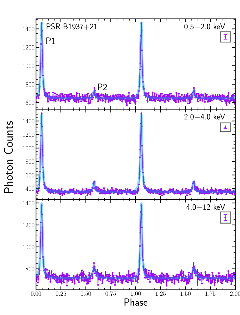
Figure 1: Phase folded pulse profiles for PSR B1937$+$21 at three different energy selections with 300 phase bins. The best fit two Lorentzian model is plotted in blue. The boxed point shows the characteristic error bar for each profile.

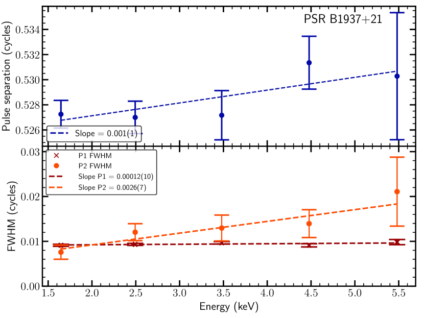
Figure 2: Evolution of pulse separation and FWHM as a function of energy for PSR B1937$+$21. A weighted linear regression is used to fit this evolution over five 1 keV-wide energy intervals whose corresponding data points were located through spectra integration.

Table 3: Pulse separation and width corresponding to Figure 2. For each energy range, we use the pulsed emission spectra from §3.2 to find the median energy. We find the slope of the pulse separation is consistent with zero.

Pulse	FWHM	FWHM	Energy	Energy
Separation	of P1	of P2	band	Median
(cycles)	(cycles)	(cycles)	(keV)	(keV)
0.527(1)	0.0091(2)	0.008(1)	$1.0-2.0$	$1.65$
0.527(1)	0.0093(2)	0.012(2)	$2.0-3.0$	$2.49$
0.527(2)	0.0097(3)	0.013(3)	$3.0-4.0$	$3.48$
0.531(2)	0.0091(4)	0.014(3)	$4.0-5.0$	$4.48$
0.530(5)	0.0098(6)	0.021(8)	$5.0-6.0$	$5.48$

3.2 Spectroscopy

We extract the source spectrum with XSELECT v.2.4 from the cleaned event files used in the previous section. All spectral analyses use the NICER redistribution matrix file and ancillary response file versions 1.02. Since the pulsed fraction is nearly 100% for this source (Ng et al., 2014) we assume that any detected photons within the off-pulse phase range are due to the X-ray background. We define the off-pulse region to be $0.20\leq\phi\leq 0.40$, and $0.7\leq\phi\leq 1.0$. We use the spectrum extracted from these phase ranges as the background spectrum in our subsequent spectral analysis.

We select the on-pulse region using the variance of the background emission. Using 100 phase bins, the phase limits of each component are chosen to be where the counts exceed 3 times the standard deviation of the background. The P1 phase region is thus $0.03\leq\phi\leq 0.10$ and the P2 phase region is $0.56\leq\phi\leq 0.61$.

We compute the difference spectra by subtracting the spectrum of the background from the spectrum of the pulsed components (e.g., Fabian & Vaughan, 2003). Since the phase range is wider for the off-pulse emission spectra, we re-scale the spectrum by adjusting the exposure time with the ratio of the two phase widths. We fit models to the spectra with XSPEC v.12.10.1 (Arnaud, 1996). Interstellar medium (ISM) absorption is set using abundances from Wilms et al. (2000) and the tbabs model. This model sets the cross-section to Vern cross-sections from Verner et al. (1996) and normalizes the total photoionization cross-section by the column density of hydrogen, $N_{\textrm{H}}$. The observed spectrum is given in Equation 2 of Wilms et al. (2000) as

$$I_{\textrm{obs}}(E)=e^{-\sigma_{\textrm{ISM}}(E)N_{\textrm{H}}}I_{\textrm{source}}(E)$$ (2)

where $\sigma_{\textrm{ISM}}$ is the energy dependent photoionization cross-section of the ISM, $N_{\textrm{H}}$ is the total hydrogen number density, and $I_{\textrm{source}}(E)$ is the intrinsic X-ray spectrum of the source.

First we model the emission spectra for the two components together, binned with 600 counts per channel. The best-fit single absorbed power-law model for the pulsed emission gives an absorbing column $N_{\textrm{H}}=(1.88\pm 0.18)\times 10^{22}$ cm^-2 and spectral index $\Gamma=0.93\pm 0.09$ with $\chi^{2}_{\nu}=0.85$ for 98 degrees of freedom (dof).

As done in previous work (e.g., Ng et al., 2014), we also consider an extra blackbody component, (powerlaw+bbody)*tbabs. The fit results in a very high temperature $kT\sim 1.1$ keV with $\chi^{2}_{\nu}=0.82$ for 96 dof. This temperature is almost certainly too large to represent a physical thermal component. NICER observations of thermally-emitting MSPs have fit blackbody temperatures at $\sim 0.1$ keV (e.g., Ray et al., 2019; Harding et al., 2019). We can obtain a reasonable fit by constraining the thermal parameter to $kT\leq 0.5$ keV and the photon index in the range $0.8<\Gamma<1.5$ (resulting in $\chi^{2}_{\nu}=0.99$ with dof$=$96). The blackbody fit with constrained parameters is slightly worse than the absorbed power-law alone. Since a blackbody component is not statistically required by the data, our results are in agreement with previous work and suggest the X-ray spectrum is dominated by nonthermal, magnetospheric emission.

With NICER’s large collecting area and timing uncertainty better than 100 ns, we can model the emission spectrum of each pulse component separately. Similar to measurement of pulse amplitude at different energies, comparison of the modeled spectra between peaks can indicate how the origin of each peak differs. This can help distinguish blended features in pulse components, as done with radio observations of PSR B1133$+$16 (Hankins et al., 1991). We also model the emission spectra between the leading and trailing edges of the primary pulse component. The comparison of pulse edge spectra has been done for bright sources, such as the Crab Pulsar (Eikenberry et al., 1996) and PSR B1509$-$58 (Rots et al., 1998), but this is the first time this analysis has been possible for PSR B1937$+$21.

For each phase selection, we fit a single absorbed power-law. For these fits, we freeze the column density at $N_{\rm{H}}=1.88\times 10^{22}$ cm^-2, the best fit value from our spectrum of pulsed emission above. Figure 3 shows the emission spectra for a variety of phase selections. For each profile region (P1, leading edge, etc.), we fit multiple phases to compare the emission spectra over narrow variations in phase. Since we find no statistically significant variation between narrow-phases in each region, we make broader comparisons between the two pulses and the leading/trailing edges of P1. The model parameters for each phase-resolved spectra are given in Table 2. All errors are quoted at the 90% confidence level.

The difference between the photon indices of the two pulses is statistically significant at the $>90\%$ confidence level. This may suggest that the underlying particle spectrum differs between the two peaks. We find that the 90% confidence intervals of the photon indices overlap for the leading and and trailing edges. Therefore the NICER modeled emission spectra does not differ significantly between the edges of the P1, suggesting a uniform emission origin for the entirety of P1.

We use the extracted NuSTAR and XMM-Newton spectra from Gotthelf & Bogdanov (2017) to model the broadband emission spectrum of PSR B1937$+$21. The NuSTAR spectrum is also a difference spectra, using the off-pulse emission as the background. The XMM-Newton data was originally presented in Ng et al. (2014) and uses nearby chip regions to extract a background spectra. Gotthelf & Bogdanov (2017) previously reported $N_{\textrm{H}}=(1.8\pm 0.3)\times 10^{22}$ cm^-2 and spectral index $\Gamma=1.16\pm 0.11$ with a $\chi^{2}_{\nu}=0.91$ for 83 dof. We use the extracted spectra from Gotthelf & Bogdanov (2017) to produce a simultaneous fit of NuSTAR, XMM-Newton, and NICER. Since we are fitting difference spectra of pulse emission, the spectra from each telescope differ by multiplicative constants. Rather than fit for these constants, we allow the normalization for each data set to remain a free parameter. We find the best-fit single absorbed power-law has a photon index $\Gamma=1.04\pm 0.08$ and a hydrogen absorbing column density $N_{\textrm{H}}=(2.00\pm 0.16)\times 10^{22}$ cm^-2 with a $\chi^{2}_{\nu}=0.95$ for 145 dof. Figure 4 plots the simultaneous fit, showing the NICER spectra index is indeed consistent with measurements made by other telescopes.

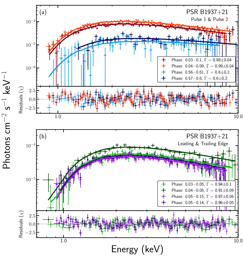
Figure 3: Emission spectra of two PSR B1937+21 pulse components (a) and leading and trailing edges of P1 (b). We fit single absorbed power-law models to each phase selection. Below each set of spectra are the residuals of the best fit powerlaw in units of $\chi$.

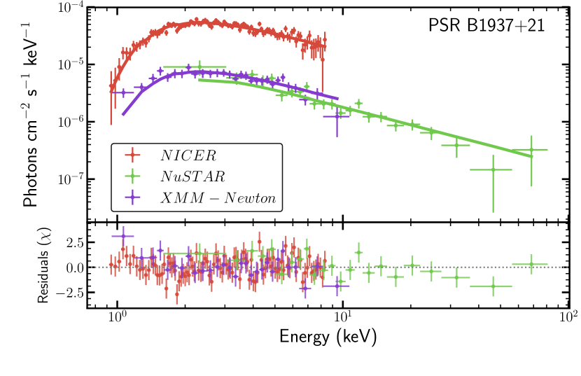
Figure 4: Top: Emission spectra of PSR B1937+21 primary pulse component fit jointly with data from NuSTAR and XMM-Newton EPIC MOS. Bottom: Residuals of the best fit power-law model.

4 PSR B1821$-$24

PSR B1821$-$24 (also known as PSR J1824$-$2452A) has a 3.05 ms period and was the first radio MSP found in a globular cluster (Lyne et al., 1987). Since then, over 150 MSPs have been detected in globular clusters. ASCA first detected the X-ray emission from this pulsar (Saito et al., 1997), with a spin-down luminosity of $\dot{E}=2.2\times 10^{36}$ erg s^-1 and a X-ray luminosity of $L=1.3\times 10^{33}$ erg s^-1. Chandra (Becker et al., 2003; Bogdanov et al., 2011), RXTE, and NuSTAR (Gotthelf & Bogdanov, 2017) have observed X-ray emission of PSR B1821$-$24. No energy dependent phase separation was observed. These studies concluded that the best fit X-ray spectral model of PSR B1821$-$24 is an absorbed power-law, indicating non-thermal emission. Gotthelf & Bogdanov (2017) performed phase-resolved spectroscopy to compare the two pulses and found them to have nearly identical photon indices. NICER observed PSR B1821$-$24 for $\leavevmode\nobreak\ \sim 715$ ks seconds between 2017-06-25 and 2019-06-30 in 271 ObsIDs.

4.1 Pulse Profiles

Table 4: Evolution of PSR B1821$-$24 P1/P2 peak ratio with respect to energy. Energy range (keV) P1/P2 0.5–2.0 2.3$\pm$0.1 2.0–4.0 2.3$\pm$0.1 4.0–12.0 2.0$\pm$0.2   Table 5: Best-fit model parameters of the absorbed single power-law for PSR B1821$-$24 emission spectra at different phase selections. Since the number of photons varies between phase selections, we use different binning when extracting the spectra, resulting in different degrees of freedom. The confidence intervals on the photon index are given at the 90% level. Region Phase Range $\Gamma$ $\chi^{2}_{\nu}$ Degrees of Number of Freedom Photons Pulse 1 0.7 – 0.78 1.12$\pm$0.05 1.11 55.0 49904 0.71 – 0.77 1.09$\pm$0.05 1.04 45.0 39679 Leading Edge 0.7 – 0.72 1.05$\pm$0.12 0.77 53.0 11995 0.71 – 0.72 0.97$\pm$0.11 0.94 45.0 6651 Trailing Edge 0.72 – 0.78 1.13$\pm$0.06 0.99 64.0 37909 0.72 – 0.77 1.11$\pm$0.05 1.29 62.0 33028 Pulse 2 0.23 – 0.34 1.14$\pm$0.08 1.02 45.0 60184 0.24 – 0.33 1.16$\pm$0.08 1.09 46.0 50489

Figure 5 plots the phase folded profiles for PSR B1821$-$24 over the three energy ranges spanning the entire NICER bandwidth. Like PSR B1937$+$21, RXTE X-ray observations show the pulsed fraction of PSR B1821$-$24 is near 100% (Ray et al., 2008).

PSR B1821$-$24 has a similar X-ray pulse profile to that of PSR B1937$+$21 with two narrow pulse components. We apply the same three-step fitting procedure described in Section §1 by fitting Lorentzians to pulse profiles with narrow energy selections. Figure 6 shows that the slope of the separation as a function of energy, $m_{sep}$ is consistent with zero in the NICER energy range. We include an additional data point for the RXTE data between $6.0$–$17.0$ keV. The x-axis value for this bin is chosen using the extracted RXTE spectrum from (Gotthelf & Bogdanov, 2017). We find the slope $m_{\rm{sep}}$ is again consistent with zero. The $95\%$ upper limit on the pulse separation of PSR B1821$-$24 is 0.00052 cycles/keV. The NICER observations are therefore a testament to the stability of the pulse profile over almost an order of magnitude of X-ray energies.

The width of both pulses is shown to decrease at the 0.8$\sigma$ confidence level for P1 and 1.5$\sigma$ for P2. The $95\%$ upper limits are 0.00022 and 0.0011, for |$m_{\rm{FWHM,P1}}$| and |$m_{\rm{FWHM,P2}}$|, respectively. Finally, we find that the ratio of the peak components P1/P2, given in Table 5, is suggestive of a decrease with increasing energy as was the case with PSR B1937$+$21.

Figure 5: Phase folded pulse profile for PSR B1821$-$24 with 300 phase bins. We fit a Lorentzian to each pulse to estimate its center and width. P2 in this profile is relatively larger than the secondary pulse for PSR B1937$+$21. Boxed point shows characteristic error bar for each profile.

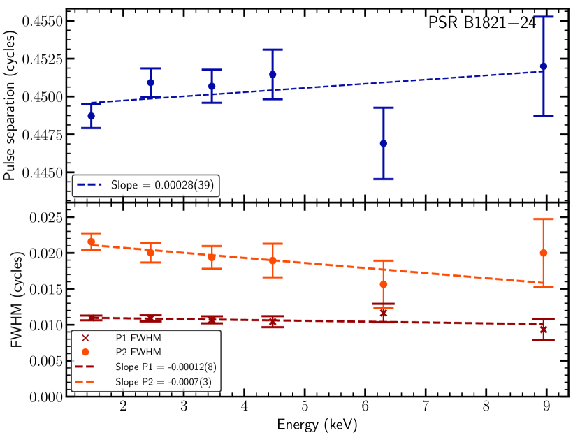
* The data-point corresponding to the NICER range $5.0-8.0$ is at $6.31$ keV through integration of the spectra. This same technique was used to locate the last data point corresponding to RXTE data at $8.95$ keV.

Figure 6: Evolution of pulse separation and FWHM as a function of energy for PSR B1821$-$24.

Table 6: Pulse separation and width corresponding to Figure 6. For each energy range, we use the pulsed emission spectra from §4.2 to find the median energy. We find the slope of the pulse separation is consistent with zero. The last energy range corresponds to RXTE data.

Pulse	FWHM	FWHM	Energy	Energy
Separation	of P1	of P2	band	Median
(cycles)	(cycles)	(cycles)	(keV)	(keV)
0.449(1)	0.0109(3)	0.021(1)	$1.0-2.0$	$1.47$
0.451(1)	0.0109(4)	0.020(1)	$2.0-3.0$	$2.45$
0.451(1)	0.0107(5)	0.019(1)	$3.0-4.0$	$3.46$
0.451(2)	0.0104(8)	0.019(2)	$4.0-5.0$	$4.47$
0.446(2)	0.0116(10)	0.016(3)	$5.0-8.0$	$6.30$
0.452(3)	0.0093(10)	0.020(5)	$6.0-17.0$	$8.95$

4.2 Spectroscopy

Following the same procedure described in 3.2, we first extract the spectrum of the pulsed emission with a minimum of 600 counts per channel. We define the off-pulse regions to be $0.38\leq\phi\leq 0.6$ and $0.9\leq\phi\leq 1.2$. Using the standard deviation of this off-pulse region in a profile with 100 phase bins, we select the P1 phase region as $0.70\leq\phi\leq 0.78$ and the P2 region as $0.23\leq\phi\leq 0.34$. The best-fit model of the observed NICER emission spectrum extracted from both P1 and P2 is a single absorbed power-law with an absorbing column $(0.40\pm 0.08)\times 10^{22}$ cm^-2 and spectral index $\Gamma=1.12\pm 0.08$ with $\chi^{2}_{\nu}=0.93$ for 101 dof.

We add a blackbody component to the absorbed power-law and find a $kT$ value too high to suggest the presence of a physical thermal component ($\sim 1$ keV). When the temperature is constrained such that $kT\leq 0.5$ keV, both the $kT$ and component normalization are consistent with zero within the $90\%$ confidence intervals. Therefore, the PSR B1821$-$24 spectrum is dominated by magnetospheric emission and the best fit model is a single absorbed power-law.

We then compare the emission spectra of each pulse component and the edges of P1. For each extracted spectrum, we fix the column density at $N_{\rm{H}}=0.38\times 10^{22}$ cm^-2, the best-fit value from the pulsed emission. Figure 7 shows the emission spectra for these phase selections. Unlike the results of PSR B1937$+$21, we find no significant difference in photon index between the spectrum of the two pulses, a result consistent with NuSTAR analysis (Gotthelf & Bogdanov, 2017). The fit photon index of the spectra from the leading and trailing edge of P1 are also consistent within the 90% confidence intervals.

We combine NICER observations with NuSTAR and RXTE extracted spectra from Gotthelf & Bogdanov (2017) to model the joint spectrum shown in Figure 8. Both the NuSTAR and RXTE emission spectra use the scaled off-pulse region as the background. We find the best-fit single absorbed power-law has a photon index $\Gamma=1.24\pm 0.05$ and a hydrogen absorbing column density $N_{\rm{H}}=0.50\pm 0.06\times 10^{22}$ cm^-2 with a $\chi^{2}_{\nu}=0.95$ for 213 dof.

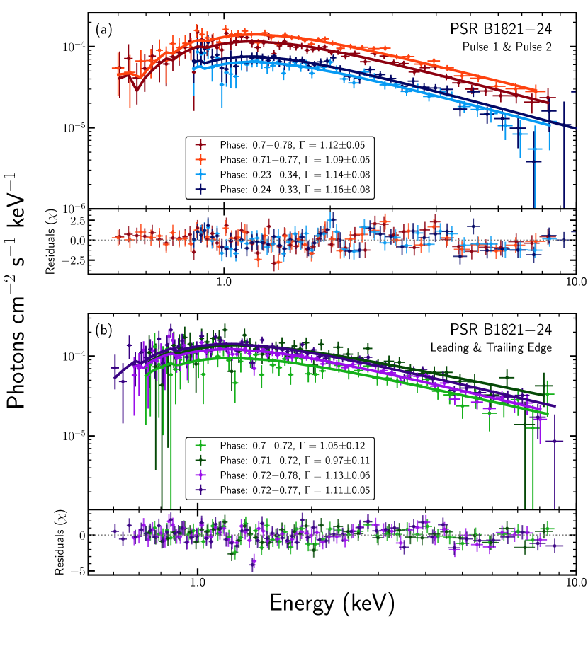
Figure 7: Emission spectra of two PSR B1821$-$24 pulse components (a) and leading and trailing edges of P1 (b). We fit a single absorbed power-law to each of the phase selections. Below each set of spectra are the residuals of the best fit power-law in units of $\chi$.

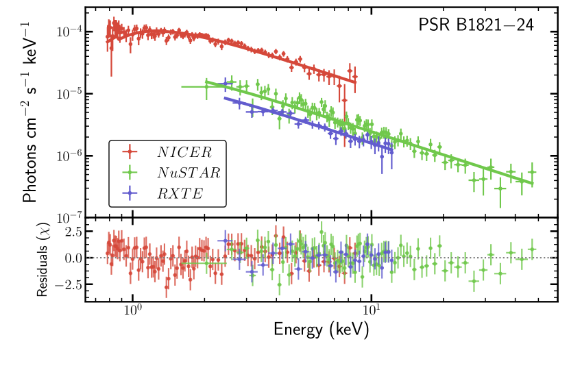
Figure 8: Top: Emission spectra of PSR B1821-24 primary pulse component fit jointly with data from NuSTAR and RXTE. Bottom: Residuals of combined fit for each spectra.

5 PSR J0218+4232

PSR J0218+4232 was first confirmed as an MSP by Navarro et al. (1995), who showed it is in a two-day orbit with a white dwarf companion. It has a 2.3 ms period and a spin down luminosity of $\dot{E}=2.4\times 10^{36}$ erg s^-1. This pulsar was detected in soft X-rays by ROSAT HRI and PSPC (Verbunt et al., 1996; Kuiper et al., 1998). These observations revealed that two-thirds of the emission between 0.1–2.4 keV is non-pulsed.

PSR J0218$+$4232 was also detected with the Energetic Gamma Ray Experiment Telescope (EGRET) onboard the Compton Gamma Ray Observatory (CGRO) (Kuiper et al., 2000). BeppoSax (Mineo et al., 2000), NuSTAR (Gotthelf & Bogdanov, 2017), and XMM-Newton (Webb et al., 2004) have continued to observe the X-ray emission of PSR J0218$+$4232. As compared to PSR B1821$-$24 and PSR B1937$+$21, the functional form of the PSR J0218$+$4232 spectra is less certain. The best fit model has been determined to be an absorbed power-law within the energy range 2–10 keV by BeppoSax (Mineo et al., 2000) and NuSTAR (Gotthelf & Bogdanov, 2017). Additionally, for the energy range of 0.2–10 keV, XMM-Newton data suggests that the model of best fit is an absorbed power-law and a blackbody (Webb et al., 2004). The variation in best fit models suggests that there may be a thermal component detected only at lower energies, possibly between 0.6–2.0 keV. NICER has observed this source for $\sim 1190$ ks between 2017-06-26 and 2019-06-23 in 282 ObsIDs.

5.1 Pulse profiles

Table 7: Evolution of PSR J0218$+$4232 P1/P2 peak ratio with respect to energy. Energy range (keV) P1/P2 0.5–2.0 1.6$\pm$0.1 2.0–4.0 1.5$\pm$0.1 4.0–12.0 1.7$\pm$0.3   Table 8: Best-fit model parameters for the single absorbed power-law $+$ Gaussian PSR J0218$+$4232 emission spectra at different phase selections. Since the number of photons varies between phase selections, we use different binning when extracting the spectra, resulting in different degrees of freedom. Region Phase Range $\Gamma$ $\chi^{2}_{\nu}$ Degrees of Number of Freedom Photons Pulse 1 0.28 – 0.54 0.99$\pm$0.04 0.88 126.0 196111 0.34 – 0.48 0.98$\pm$0.04 0.89 80.0 112050 Leading Edge 0.28 – 0.41 1.02$\pm$0.06 0.82 88.0 97242 0.34 – 0.41 0.98$\pm$0.06 0.93 52.0 55150 Trailing Edge 0.41 – 0.54 0.96$\pm$0.06 1.30 83.0 98869 0.41 – 0.48 0.95$\pm$0.06 0.99 49.0 56900 Pulse 2 0.79 – 1.03 0.92$\pm$0.07 0.99 104.0 171697 0.85 – 0.97 0.9$\pm$0.07 0.99 61.0 89814 Leading Edge 0.79 – 0.91 0.78$\pm$0.1 1.19 67.0 85255 0.85 – 0.91 0.76$\pm$0.09 1.16 37.0 44867 Trailing Edge 0.91 – 1.03 1.03$\pm$0.08 0.92 67.0 86442 0.91 – 0.97 0.94$\pm$0.09 0.92 38.0 44947

The phase folded pulse profile, shown in Figure 9, is much broader than those of the other two pulsars presented in this paper. There is evidence for an emission bridge connecting the two pulses. Unlike the pulses of the other two pulsars, the pulses of PSR J0218$+$4232 are best fit by Gaussians rather than Lorentzians.

As before, we utilize a three-step fitting process. We first fit two Gaussians to the pulse profile at six energy subsets between 0.2–6.2 keV. We then monitor the evolution of pulse separation with slopes $m_{\rm{sep}}$, $m_{\rm{FWHM,P1}}$, and $m_{\rm{FWHM,P2}}$. Figure 10 shows the results of our fitting procedure.

We find a significant decrease in pulse separation at the 3.7$\sigma$ level with higher energies. A detailed discussion of these results is offered in section 6. This is the first detection of energy dependent pulse separation in PSR J0218$+$4232 X-ray observations.

We find that the slopes corresponding to each pulse width, $m_{\rm{FWHM,P1}}$ and $m_{\rm{FWHM,P2}}$, are consistent with zero for both P1 and P2. We find the $95\%$ upper limit for width evolution is 0.00071 cycles/keV for |$m_{\rm{FWHM,P1}}$| and 0.0012 cycles/keV for |$m_{\rm{FWHM,P2}}$|.

Table 8 shows our measurement of the ratio P1/P2 is consistent with no change with energy, although a higher signal-to-noise measurement could reveal a trend.

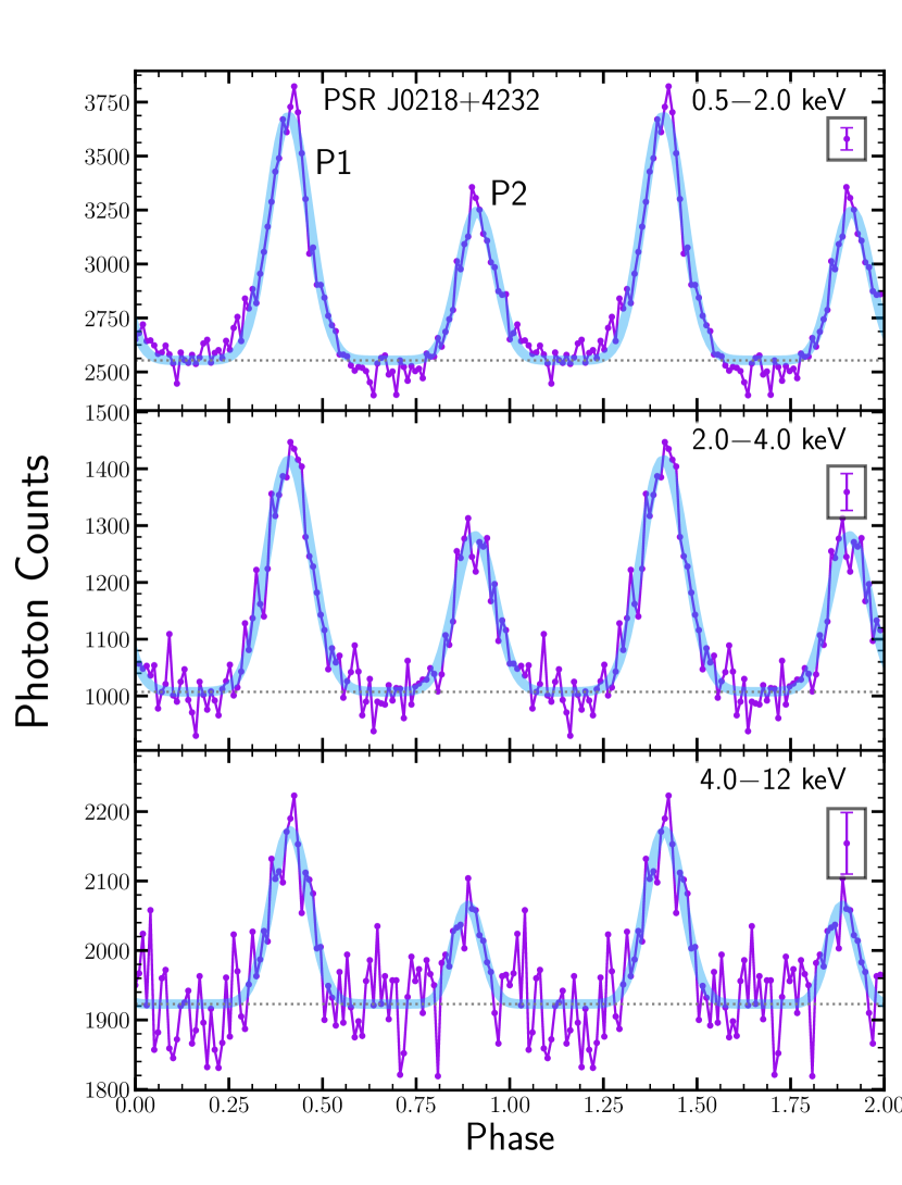
Figure 9: Phase folded pulse profile for PSR J0218$+$4232 with 100 phase bins. We fit Gaussians to each component to estimate its center and width. The pulse components are broader as compared to the other observed pulsars. The boxed point shows the characteristic error bar for each profile. The gray dotted line represents the vertical offset when fitting the double Gaussian model.

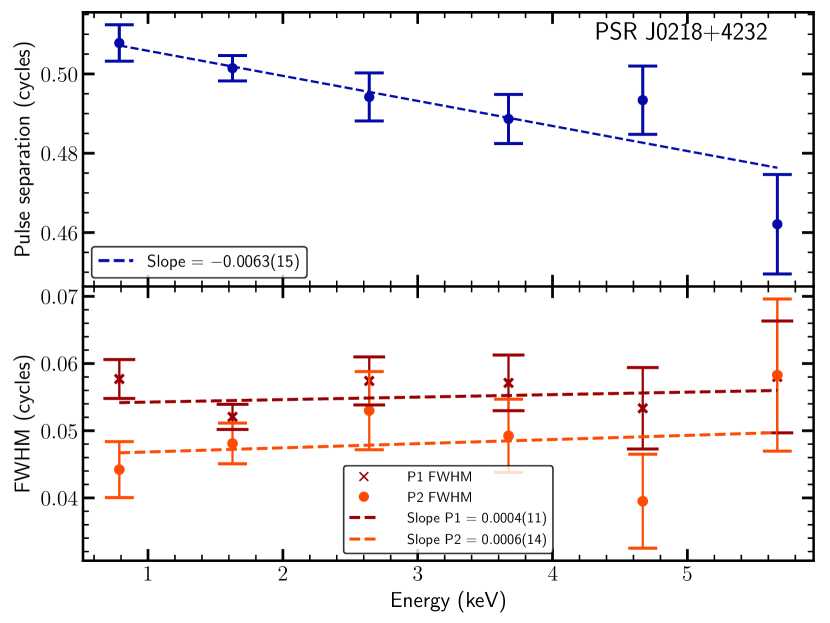
Figure 10: Evolution of pulse separation and FWHM as a function of energy for PSR J0218$+$4232

Table 9: Pulse separation and width corresponding to Figure 10. For each energy range, we use the pulsed emission spectra from §5.2 to find the median energy. We find the slope of the pulse separation is significant at the 3.7 $\sigma$ level.

Pulse	FWHM	FWHM	Energy	Energy
Separation	of P1	of P2	band	Median
(cycles)	(cycles)	(cycles)	(keV)	(keV)
0.508(4)	0.058(3)	0.044(4)	$0.2-1.2$	$0.79$
0.501(3)	0.052(2)	0.048(3)	$1.2-2.2$	$1.63$
0.494(6)	0.057(3)	0.053(6)	$2.2-3.2$	$2.64$
0.489(6)	0.057(4)	0.049(5)	$3.2-4.2$	$3.67$
0.493(9)	0.053(6)	0.039(7)	$4.2-5.2$	$4.67$
0.462(12)	0.058(5)	0.058(11)	$5.2-6.2$	$5.67$

5.2 Spectroscopy

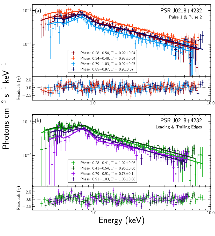
Figure 11: Emission spectra of two PSR J0218$+$4232 pulse components (a) and leading and trailing edges of P1 and P2 (b). We fit single absorbed power-laws with a Gaussian emission line to each phase selection. Below each set of spectra are the residuals of the model in units of $\chi$.

Since the pulsed fraction is only $\sim 65\%$ for this source (Zavlin, 2007), we can not rely on the off-pulse region for our selecting the phase boundaries when extracting our spectra. Instead, we use the Gaussian fitted parameters from the previous section to determine the centers and widths of the pulses. We first extract the spectrum between phases $0.28\leq\phi\leq 0.54$ for P1 and $0.79\leq 1.03$ for P2. Since the phase ranges are wider for this pulsar, and the exposure time is greater, we group the extracted spectra with minimum 2500 counts/bin while maintaining similar energy resolution per bin as the other pulsars.

Rather than defining a narrow off-pulse region to extract a background spectrum, we use a space-weather background generated based on the geomagnetic index $K_{p}$ and cutoff rigidity COR_SAX. We first fit a single absorbed power-law to the combined P1$+$P2 pulsed emission. The HI column density is fixed at $N_{H}=6.75\times 10^{20}$ cm^-2, the value from HI4PI Collaboration et al. (2016). The best fit has a photon index $\Gamma=1.19$ with a high $\chi^{2}_{\nu}=1.93$ for 84 dof. Since this background is based on the GTIs used in the extracted spectra, our background subtracted spectra still shows residual features at $<1.0$ keV, possibly due to ionized oxygen emission. This feature, likely an emission line originating in the Solar wind or local hot bubble, has been observed in NICER spectra before (Ray et al., 2019).

In order to improve upon the fit, we add an additional Gaussian component. The best fit tbabs*(powerlaw+gaussian) model has photon index $\Gamma=1.05\pm 0.05$, line center $l_{E}=0.80\pm 0.03$ keV, and line width $\sigma_{E}=0.11\pm 0.03$ keV resulting in a $\chi^{2}_{\nu}=0.88$ for 82 dof.

We then fit the spectrum extracted from narrow phase regions, including both pulses and their leading/trailing edges. For each model, we freeze the $l_{E}$ and $\sigma_{E}$ at the values listed above because the foreground emission component is not expected to vary significantly between phase selections. Figure 11 plots the emission spectra with the tbabs*(powerlaw+gaussian) model for each phase selection. Table 8 gives the model fits for each phase range. While our results seem to suggest that the P1 photon index is higher than that of P2, we find that whether or not the confidence intervals overlap depends on the phase selections used.

Finally, we fit the NICER extracted spectrum alongside NuSTAR and XMM-Newton observations from Gotthelf & Bogdanov (2017). The XMM-Newton spectra was originally presented in (Webb et al., 2004) and uses a off-source image for the background spectra. The NuSTAR spectra uses a phase averaged background spectra. Again, we fix the column density $N_{\rm{H}}=6.75\times 10^{20}$ cm^-2. The best fit single-absorbed power-law has a photon index $\Gamma=1.18\pm 0.03$ with a $\chi^{2}_{\nu}=1.47$ for 154 dof. We also fit the tbabs*(powerlaw+Gaussian) model, freezing the Gaussian component parameters at zero for the NuSTAR and XMM-Newton data. The best-fit model has a photon index $\Gamma=1.10\pm 0.04$ with a $\chi^{2}_{\nu}=1.06$ for 151 dof. Figure 12 plots the simultaneous fit of these three telescopes.

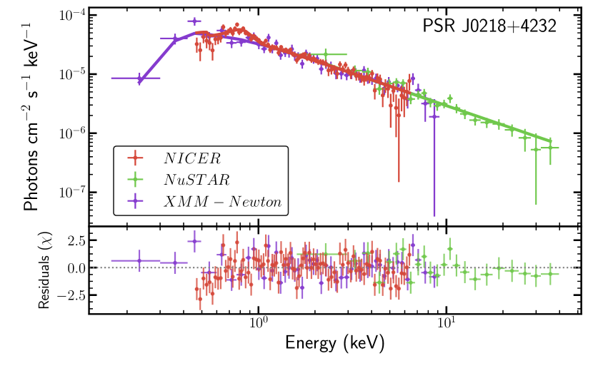
Figure 12: Top: Emission spectra of PSR J0218$+$4232 extracted from both pulses fit jointly with data from NuSTAR and XMM-Newton. Bottom: Residuals of the joint model fit for each spectra.

6 Discussion & Conclusions

We present two years of NICER soft X-ray observations of three energetic MSPs: PSRs B1937$+$21, B1821$-$24, and J0218$+$4232. We use the high precision timing measurements to track pulse profile evolution at different energies and model phase-resolved emission spectra.

Table 10 summarizes the results of the analysis of profile evolution with energy for the three pulsars. We find that the decrease of pulse separation is significant at $>3.7\sigma$ for PSR J0218$+$4232 in the NICER energy range. This is the first evidence for the evolution of pulse profile separation in the soft X-ray regime for this pulsar.

While pulse profile morphology has been studied extensively in radio observations (e.g., Rankin, 1983), few pulsars are bright enough for detailed measurements at higher energies. Observations of the Vela pulsar (PSR J0835$-$4510) with the Large Area Telescope on Fermi have revealed constant pulse separation between pulse 1 and pulse 2 and an increasing separation between pulse 1 and pulse 3 as a function of energy. The widths of all three pulses were found to decrease (Abdo et al., 2010a). Observations of the Crab Pulsar have shown similar results of no phase shift with energy and decreasing pulse width (Abdo et al., 2010b).

The energy dependence of pulse separation for PSR J0218$+$4232 suggests that regions characterized by slightly higher particle energies, larger local magnetic fields, or larger pitch angles map to slightly different phases of the observed light curve than the lower-energy radiation. Our viewing angle could be such that P1 and P2 could originate near the same side of the CS associated with one magnetic pole. In this case, the higher-energy emission originates slightly farther from the CS center compared to the lower-energy emission. The magnetic field lines going into the CS map back to the return current region on one polar cap (Timokhin & Arons, 2013; Harding et al., 2018). On the other hand, if P1 and P2 originate from opposite poles, then they come from opposite sides of the respective CSs, with higher-energy particles again originating farther from the CS center for the two-pole model to be consistent with the peaks’ frequency-dependent shift (see e.g. Figure 10 in Bai & Spitkovsky 2010).

We find no evidence for energy-dependent pulse separation in PSR B1937$+$21 and PSR B1821$-$24 and place constraints on the X-ray pulse separation evolution. A higher instrumental sensitivity could reveal energy-dependent separations for these pulsars.

Our results for FWHM evolution suggest that pulse width increases in PSR B1937$+$21 and decreases in PSR B1821$-$24 at confidence levels ranging from 0.8 $\sigma$ to 2.6 $\sigma$, while it remains constant across the NICER energy regime for PSR J0218$+$4232.

Table 10: Slopes of the linear regression of pulse separation and FWHM with respect to energy.

PSR	Pulse Separation	FWHM of P1	FWHM of P2
B1937$+$21	0.001(1)	0.00012(10)	0.0026(7)
B1821$-$24	0.00028(39)	$-$0.00012(8)	$-$0.0007(3)
J0218$+$4232	$-$0.0063(15)	0.0004(11)	0.0006(14)

The errors correspond to the 1-$\sigma$ Gaussian standard deviations.

Spectral analyses are consistent with the hard power-law emission spectra expected for these three pulsars. With over 1000 ks of exposure for PSRs B1937$+$21 and J0218$+$4232 and over 700 ks of exposure for PSR B1821$-$24, NICER observations contribute to the wealth of X-ray observations used to model the emission spectra of these pulsars. We provide updated model parameters of the single absorbed power-law for each pulsar and find no evidence of additional black body components for PSRs B1937$+$21 and B1821$-$24. We observe an additional emission line feature at $<1.0$ keV for PSR J0218$+$4232 unfit by the instrument response. This limitation prevents accurate evaluation of black body components for this pulsar.

For PSR B1937$+$21, we observe different emission spectra photon indices at $>2\sigma$ level. Observation of different photon indices for different pulse profile peaks suggests that the particle spectrum varies between phases. This may be due to slightly different local conditions such as the magnetic field strengths and pitch angles, or different pair injection spectra, which influence the dynamics and radiation by these particles. We do not observe this behavior for PSR B1821$-$24, suggesting a similar emission origin or local conditions for each peak.

Though the majority of equatorial CS models pertain to gamma-ray emission (e.g. Cerutti et al., 2016; Kalapotharakos et al., 2014), we note that the pulsars presented here have pulse features that are aligned across radio, X-ray, and gamma-ray observations. In the case of PSR B1937$+$21, a close phase alignment between radio giant pulses and X-ray emission has been observed (Cusumano et al., 2003), motivating NICER correlation searches that will be reported in a separate paper. Profiles that are phase-aligned across wavebands may point to (nearly) overlapping spatial emission origins for the different bands. The closer the overlap in altitude and extent of these regions, the closer the phase-alignment across bands. In earlier gap models, such as slot gap (Muslimov & Harding, 2004) and outer gap (Romani & Yadigaroglu, 1995), the special relativistic effects of aberration and time-of-flight delay plus the magnetic field geometry (Dyks et al., 2004) affect photons of different energies in the same way to produce caustics in the emission sky maps. In more modern global magnetosphere models, caustics form due to stagnation of emission directions as a result of the magnetic field geometry in the CS (Bai & Spitkovsky, 2010). While the origin of the caustics is qualitatively different in these models, the argument of similar spatial origin of photons seen at similar observational phases continues to hold.

The present X-ray observations thus probe both the emission geometry and spatial properties of the plasma in the CS, which will be augmented as future models will attempt to produce the correct peak phases in many different wavebands.

Appendix A Different Profile Fitting Methods

We used a variety of functional models to fit the pulse profile components in our study of profile evolution. The simplest model is a symmetrical Gaussian for each component (Kramer et al., 1994). We use this model as a basis to compare other functional forms. By eye, the pulse components of PSRs B1937$+$21 and B1821$-$24 appear slightly asymmetrical. Profile modeling of Chandra (Ng et al., 2014) and Fermi (Abdo et al., 2013) observations used a sum of two asymmetrical Lorentzians. Some sources suggest that the asymmetrical pulse component is due to giant pulse emission at the trailing edge (Romani & Johnston, 2001), motivating the implementation of a triple Gaussian model. Figure 13 plots each of the aforementioned functional forms for PSR B1937$+$21’s pulse components. The triple-Gaussian model was discarded for being overly dependent on initial conditions and thus unable to give a repeatable fit. Repeating the fitting procedure with different initial conditions for the third Gaussian component led to different results. Only the symmetrical and asymmetrical Gaussians and Lorentzians were compared. Because the asymmetrical functions were made nearly symmetrical by the parameter optimization algorithm, a $\chi^{2}$ analysis proved the addition of the skewness parameters to be inefficient. Over the five energy ranges for PSRs B1937$+$21 and B1821$-$24, symmetrical Lorentzians outperformed symmetrical Gaussians with a significantly smaller $\chi^{2}$ value and were therefore chosen for our pulse profile analysis. For the PSR J0218$+$4232 pulse profile, the Gaussian fits to each pulse are a better fit and were used in the analysis of this pulsar.

For each of these models, we compared the measurements of pulse component evolution with energy. We found that results for each pulsar are consistent across choice of model and phase binning. Table 11 shows no significant change in the slopes of profile feature evolution with energy for PSR J0218$+$4232 when adding more phase bins. Our results are thus independent of phase binning.

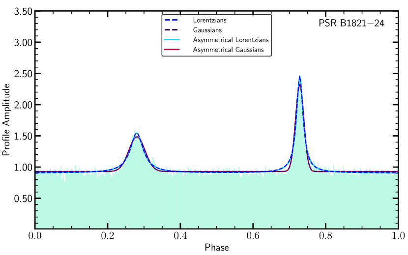
Figure 13: Fitting the PSR B1821$-$24 pulse profile against different functional forms in the 1.0–2.0 keV energy band.

Number of phase bins	$m_{\rm{sep}}$	$m_{\rm{FWHM,P1}}$	$m_{\rm{FWHM,P2}}$
50	-0.0066(15)	0.0004(10)	0.0006(13)
100	-0.0063(15)	0.0004(11)	0.0006(14)
300	-0.0063(14)	0.0002(13)	0.0005(15)

Table 11: Comparison of profile feature slopes for PSR J0218$+$4232 using different numbers of phase bins.

References

- Abdo et al. (2010a) Abdo, A. A., Ackermann, M., Ajello, M., et al. 2010a, ApJ, 713, 154, doi: 10.1088/0004-637X/713/1/154
- Abdo et al. (2010b) —. 2010b, ApJ, 708, 1254, doi: 10.1088/0004-637X/708/2/1254
- Abdo et al. (2013) Abdo, A. A., Ajello, M., Allafort, A., et al. 2013, ApJS, 208, 17, doi: 10.1088/0067-0049/208/2/17
- Ansoldi et al. (2016) Ansoldi, S., Antonelli, L. A., Antoranz, P., et al. 2016, A&A, 585, A133, doi: 10.1051/0004-6361/201526853
- Arnaud (1996) Arnaud, K. A. 1996, in Astronomical Society of the Pacific Conference Series, Vol. 101, Astronomical Data Analysis Software and Systems V, ed. G. H. Jacoby & J. Barnes, 17
- Arons (1983) Arons, J. 1983, ApJ, 266, 215, doi: 10.1086/160771
- Backer et al. (1982) Backer, D. C., Kulkarni, S. R., Heiles, C., Davis, M. M., & Goss, W. M. 1982, Nature, 300, 615, doi: 10.1038/300615a0
- Bai & Spitkovsky (2010) Bai, X.-N., & Spitkovsky, A. 2010, ApJ, 715, 1282, doi: 10.1088/0004-637X/715/2/1282
- Bartels et al. (1939) Bartels, J., Heck, N. H., & Johnston, H. F. 1939, Terrestrial Magnetism and Atmospheric Electricity (Journal of Geophysical Research), 44, 411, doi: 10.1029/TE044i004p00411
- Becker & Trümper (1993) Becker, W., & Trümper, J. 1993, Nature, 365, 528, doi: 10.1038/365528a0
- Becker & Trümper (1999) —. 1999, A&A, 341, 803. https://arxiv.org/abs/astro-ph/9806381
- Becker et al. (2003) Becker, W., Swartz, D. A., Pavlov, G. G., et al. 2003, ApJ, 594, 798, doi: 10.1086/376967
- Bhattacharya & van den Heuvel (1991) Bhattacharya, D., & van den Heuvel, E. P. J. 1991, Phys. Rep., 203, 1, doi: 10.1016/0370-1573(91)90064-S
- Bogdanov et al. (2011) Bogdanov, S., van den Berg, M., Servillat, M., et al. 2011, ApJ, 730, 81, doi: 10.1088/0004-637X/730/2/81
- Brambilla et al. (2018) Brambilla, G., Kalapotharakos, C., Timokhin, A. N., Harding, A. K., & Kazanas, D. 2018, ApJ, 858, 81, doi: 10.3847/1538-4357/aab3e1
- Cerutti et al. (2016) Cerutti, B., Philippov, A. A., & Spitkovsky, A. 2016, MNRAS, 457, 2401, doi: 10.1093/mnras/stw124
- Cheng et al. (1986) Cheng, K. S., Ho, C., & Ruderman, M. 1986, ApJ, 300, 500
- Cusumano et al. (2003) Cusumano, G., Hermsen, W., Kramer, M., et al. 2003, A&A, 410, L9, doi: 10.1051/0004-6361:20031368
- Deneva et al. (2019) Deneva, J. S., Ray, P. S., Lommen, A., et al. 2019, arXiv e-prints, arXiv:1902.07130. https://arxiv.org/abs/1902.07130
- Durant et al. (2012) Durant, M., Kargaltsev, O., Pavlov, G. G., et al. 2012, ApJ, 746, 6, doi: 10.1088/0004-637X/746/1/6
- Dyks et al. (2004) Dyks, J., Harding, A. K., & Rudak, B. 2004, ApJ, 606, 1125, doi: 10.1086/383121
- Dyks & Rudak (2003) Dyks, J., & Rudak, B. 2003, ApJ, 598, 1201, doi: 10.1086/379052
- Eikenberry & Fazio (1997) Eikenberry, S. S., & Fazio, G. G. 1997, ApJ, 476, 281, doi: 10.1086/303616
- Eikenberry et al. (1996) Eikenberry, S. S., Fazio, G. G., Ransom, S. M., et al. 1996, ApJ, 467, L85, doi: 10.1086/310206
- Eilek & Hankins (2016) Eilek, J. A., & Hankins, T. H. 2016, Journal of Plasma Physics, 82, 635820302, doi: 10.1017/S002237781600043X
- Fabian & Vaughan (2003) Fabian, A. C., & Vaughan, S. 2003, MNRAS, 340, L28, doi: 10.1046/j.1365-8711.2003.06465.x
- Ge et al. (2016) Ge, M. Y., Yan, L. L., Lu, F. J., et al. 2016, ApJ, 818, 48, doi: 10.3847/0004-637X/818/1/48
- Gendreau & Arzoumanian (2017) Gendreau, K., & Arzoumanian, Z. 2017, Nature Astronomy, 1, 895, doi: 10.1038/s41550-017-0301-3
- Gotthelf & Bogdanov (2017) Gotthelf, E. V., & Bogdanov, S. 2017, ApJ, 845, 159, doi: 10.3847/1538-4357/aa813c
- Guillemot et al. (2012) Guillemot, L., Johnson, T. J., Venter, C., et al. 2012, ApJ, 744, 33, doi: 10.1088/0004-637X/744/1/33
- Guillot et al. (2019) Guillot, S., Pavlov, G. G., Reyes, C., et al. 2019, ApJ, 874, 175, doi: 10.3847/1538-4357/ab0f38
- Hankins et al. (1991) Hankins, T. H., Izvekova, V. A., Malofeev, V. M., et al. 1991, ApJ, 373, L17, doi: 10.1086/186041
- Harding et al. (2019) Harding, A., Enoto, T., Kobayaashi, S., et al. 2019, in AAS/High Energy Astrophysics Division, AAS/High Energy Astrophysics Division, 111.10
- Harding & Kalapotharakos (2015) Harding, A. K., & Kalapotharakos, C. 2015, ApJ, 811, 63, doi: 10.1088/0004-637X/811/1/63
- Harding et al. (2018) Harding, A. K., Kalapotharakos, C., Barnard, M., & Venter, C. 2018, The Astrophysical Journal, 869, L18, doi: 10.3847/2041-8213/aaf3b2
- Harding & Muslimov (2001) Harding, A. K., & Muslimov, A. G. 2001, ApJ, 556, 987, doi: 10.1086/321589
- HI4PI Collaboration et al. (2016) HI4PI Collaboration, Ben Bekhti, N., Flöer, L., et al. 2016, A&A, 594, A116, doi: 10.1051/0004-6361/201629178
- Hobbs et al. (2010) Hobbs, G., Archibald, A., Arzoumanian, Z., et al. 2010, Classical and Quantum Gravity, 27, 084013, doi: 10.1088/0264-9381/27/8/084013
- Johnson et al. (2013) Johnson, T. J., Guillemot, L., Kerr, M., et al. 2013, ApJ, 778, 106, doi: 10.1088/0004-637X/778/2/106
- Johnson et al. (2014) Johnson, T. J., Venter, C., Harding, A. K., et al. 2014, ApJS, 213, 6, doi: 10.1088/0067-0049/213/1/6
- Kalapotharakos et al. (2018) Kalapotharakos, C., Brambilla, G., Timokhin, A., Harding, A. K., & Kazanas, D. 2018, ApJ, 857, 44, doi: 10.3847/1538-4357/aab550
- Kalapotharakos et al. (2014) Kalapotharakos, C., Harding, A. K., & Kazanas, D. 2014, ApJ, 793, 97, doi: 10.1088/0004-637X/793/2/97
- Kramer et al. (1994) Kramer, M., Wielebinski, R., Jessner, A., Gil, J. A., & Seiradakis, J. H. 1994, A&AS, 107, 515
- Kramer et al. (1998) Kramer, M., Xilouris, K. M., Lorimer, D. R., et al. 1998, ApJ, 501, 270, doi: 10.1086/305790
- Kuiper et al. (1998) Kuiper, L., Hermsen, W., Verbunt, F., & Belloni, T. 1998, A&A, 336, 545
- Kuiper et al. (2000) Kuiper, L., Hermsen, W., Verbunt, F., et al. 2000, A&A, 359, 615. https://arxiv.org/abs/astro-ph/0005338
- Lorimer (2008) Lorimer, D. R. 2008, Living Reviews in Relativity, 11, 8, doi: 10.12942/lrr-2008-8
- Lyne et al. (1987) Lyne, A. G., Brinklow, A., Middleditch, J., Kulkarni, S. R., & Backer, D. C. 1987, Nature, 328, 399, doi: 10.1038/328399a0
- Mineo et al. (2000) Mineo, T., Cusumano, G., Kuiper, L., et al. 2000, A&A, 355, 1053
- Mukerjee et al. (1999) Mukerjee, K., Agrawal, P. C., Paul, B., et al. 1999, Bulletin of the Astronomical Society of India, 27, 181
- Muslimov & Harding (2003) Muslimov, A. G., & Harding, A. K. 2003, ApJ, 588, 430, doi: 10.1086/368162
- Muslimov & Harding (2004) —. 2004, ApJ, 606, 1143, doi: 10.1086/383079
- Nasa High Energy Astrophysics Science Archive Research Center (2014) (Heasarc) Nasa High Energy Astrophysics Science Archive Research Center (Heasarc). 2014, HEAsoft: Unified Release of FTOOLS and XANADU, Astrophysics Source Code Library. http://ascl.net/1408.004
- Navarro et al. (1995) Navarro, J., de Bruyn, A. G., Frail, D. A., Kulkarni, S. R., & Lyne, A. G. 1995, ApJ, 455, L55, doi: 10.1086/309816
- Ng et al. (2014) Ng, C. Y., Takata, J., Leung, G. C. K., Cheng, K. S., & Philippopoulos, P. 2014, ApJ, 787, 167, doi: 10.1088/0004-637X/787/2/167
- Nicastro et al. (2004) Nicastro, L., Cusumano, G., Löhmer, O., et al. 2004, A&A, 413, 1065, doi: 10.1051/0004-6361:20031593
- Okajima et al. (2016) Okajima, T., Soong, Y., Balsamo, E. R., et al. 2016, in Society of Photo-Optical Instrumentation Engineers (SPIE) Conference Series, Vol. 9905, Space Telescopes and Instrumentation 2016: Ultraviolet to Gamma Ray, 99054X, doi: 10.1117/12.2234436
- Philippov & Spitkovsky (2018) Philippov, A. A., & Spitkovsky, A. 2018, ApJ, 855, 94, doi: 10.3847/1538-4357/aaabbc
- Pravdo et al. (1997) Pravdo, S. H., Angelini, L., & Harding, A. K. 1997, ApJ, 491, 808, doi: 10.1086/304996
- Prigozhin et al. (2016) Prigozhin, G., Gendreau, K., Doty, J. P., et al. 2016, in Society of Photo-Optical Instrumentation Engineers (SPIE) Conference Series, Vol. 9905, Space Telescopes and Instrumentation 2016: Ultraviolet to Gamma Ray, 99051I, doi: 10.1117/12.2231718
- Rangelov et al. (2017) Rangelov, B., Pavlov, G. G., Kargaltsev, O., et al. 2017, ApJ, 835, 264, doi: 10.3847/1538-4357/835/2/264
- Rankin (1983) Rankin, J. M. 1983, ApJ, 274, 333, doi: 10.1086/161450
- Rankin et al. (2017) Rankin, J. M., Archibald, A., Hessels, J., et al. 2017, ApJ, 845, 23, doi: 10.3847/1538-4357/aa7b73
- Ray et al. (2008) Ray, P. S., Wolff, M. T., Demorest, P., et al. 2008, in American Institute of Physics Conference Series, Vol. 983, 40 Years of Pulsars: Millisecond Pulsars, Magnetars and More, ed. C. Bassa, Z. Wang, A. Cumming, & V. M. Kaspi, 157–159, doi: 10.1063/1.2900134
- Ray et al. (2019) Ray, P. S., Guillot, S., Ransom, S. M., et al. 2019, ApJ, 878, L22, doi: 10.3847/2041-8213/ab2539
- Riley et al. (2019) Riley, T. E., Watts, A. L., Bogdanov, S., et al. 2019, ApJ, 887, L21, doi: 10.3847/2041-8213/ab481c
- Romani & Johnston (2001) Romani, R. W., & Johnston, S. 2001, ApJ, 557, L93, doi: 10.1086/323415
- Romani & Yadigaroglu (1995) Romani, R. W., & Yadigaroglu, I. A. 1995, ApJ, 438, 314, doi: 10.1086/175076
- Rots et al. (1998) Rots, A. H., Jahoda, K., Macomb, D. J., et al. 1998, ApJ, 501, 749, doi: 10.1086/305836
- Saito et al. (1997) Saito, Y., Kawai, N., Kamae, T., et al. 1997, ApJ, 477, L37, doi: 10.1086/310512
- Takahashi et al. (2001) Takahashi, M., Shibata, S., Torii, K., et al. 2001, ApJ, 554, 316, doi: 10.1086/321330
- Timokhin & Arons (2013) Timokhin, A. N., & Arons, J. 2013, MNRAS, 429, 20, doi: 10.1093/mnras/sts298
- Venter & Harding (2014) Venter, C., & Harding, A. K. 2014, Astronomische Nachrichten, 335, 268, doi: 10.1002/asna.201312030
- Venter et al. (2012) Venter, C., Johnson, T. J., & Harding, A. K. 2012, ApJ, 744, 34, doi: 10.1088/0004-637X/744/1/34
- Verbunt et al. (1996) Verbunt, F., Johnston, H. M., de Bruyn, A. G., & van der Klis, M. 1996, in Astronomical Society of the Pacific Conference Series, Vol. 105, IAU Colloq. 160: Pulsars: Problems and Progress, ed. S. Johnston, M. A. Walker, & M. Bailes, 353
- Verner et al. (1996) Verner, D. A., Ferland, G. J., Korista, K. T., & Yakovlev, D. G. 1996, ApJ, 465, 487, doi: 10.1086/177435
- Webb et al. (2004) Webb, N. A., Olive, J. F., & Barret, D. 2004, A&A, 417, 181, doi: 10.1051/0004-6361:20040032
- Wilms et al. (2000) Wilms, J., Allen, A., & McCray, R. 2000, ApJ, 542, 914, doi: 10.1086/317016
- Zavlin (2007) Zavlin, V. E. 2007, Ap&SS, 308, 297, doi: 10.1007/s10509-007-9297-y
- Zavlin et al. (2002) Zavlin, V. E., Pavlov, G. G., Sanwal, D., et al. 2002, ApJ, 569, 894, doi: 10.1086/339351