Scaling K2. I. Revised Parameters for 222,088 K2 Stars and a K2 Planet Radius Valley at 1.9 $R_{\oplus}$

Abstract

Previous measurements of stellar properties for K2 stars in the Ecliptic Plane Input Catalog (EPIC; Huber et al., 2016) largely relied on photometry and proper motion measurements, with some added information from available spectra and parallaxes. Combining Gaia DR2 distances with spectroscopic measurements of effective temperatures, surface gravities, and metallicities from the Large Sky Area Multi-Object Fibre Spectroscopic Telescope (LAMOST) DR5, we computed updated stellar radii and masses for 26,838 K2 stars. For 195,250 targets without a LAMOST spectrum, we derived stellar parameters using random forest regression on photometric colors trained on the LAMOST sample. In total, we measured spectral types, effective temperatures, surface gravities, metallicities, radii, and masses for 222,088 A, F, G, K, and M-type K2 stars. With these new stellar radii, we performed a simple reanalysis of 299 confirmed and 517 candidate K2 planet radii from Campaigns 1–13, elucidating a distinct planet radius valley around $1.9\,R_{\oplus}$, a feature thus far only conclusively identified with Kepler planets, and tentatively identified with K2 planets. These updated stellar parameters are a crucial step in the process toward computing K2 planet occurrence rates.

1 Introduction

The ubiquity of exoplanets in the Galaxy has been established by NASA’s Kepler Telescope (Borucki et al., 2010), with the discovery of thousands of confirmed and candidate planets in both the Kepler prime and subsequent K2 missions. After the failure of two reaction wheels on Kepler, the K2 mission was commissioned, which allowed the Kepler spacecraft to stare at different fields along the ecliptic plane for approximately 80 days at a time, using radiation pressure from the Sun to act as a third stabilization axis (Howell et al., 2014).

Our knowledge of the hundreds of confirmed and candidate planets discovered in the K2 data relies on accurate and precise stellar radius measurements for their host stars. In large surveys of hundreds of thousands of stars, like K2, it is practical to rely on stellar properties derived from readily available data. The values for K2 targets in the Ecliptic Planet Input Catalog (EPIC) come from Huber et al. (2016), which were measured with galclassify, which uses the Galaxia synthetic Milky Way model (Sharma et al., 2011) and the Padova isochrones (Girardi et al., 2000; Marigo & Girardi, 2007; Marigo et al., 2008). The input sources to galclassify were reduced proper motions, spectra from the Large Sky Area Multi-Object Fiber Spectroscopic Telescope DR1 (LAMOST; Luo et al., 2015), the Radial Velocity Experiment DR4 (RAVE; Kordopatis et al., 2013), and Apache Point Observatory Galactic Evolution Experiment DR12 (APOGEE; Alam et al., 2015), parallax measurements from Hipparcos (van Leeuwen, 2007), and photometric measurements from the US Naval Observatory CCD Astrograph Catalog (UCAC4; Zacharias et al., 2013), the Sloan Digital Sky Survey (SDSS; Skrutskie et al., 2006), and the Two Micron All Sky Survey (2MASS; Skrutskie et al., 2006). For K2 Campaigns 1–8, 81% of the stars were characterized using colors and reduced proper motions, 11% from colors only, 7% from spectroscopy, and 1% from parallaxes and colors (Huber et al., 2016).

Since the EPIC was released, the European Space Agency’s Gaia mission (Gaia Collaboration et al., 2016) has now measured parallaxes for over 1.3 billion sources in DR2 (Gaia Collaboration et al., 2018). Subsequently, Berger et al. (2018) revised the radii of Kepler stars and planets, reducing typical uncertainties on those measurements by a factor of 4–5 in most cases. Measurements of stellar parameters in the EPIC were largely based on photometry and proper motions, which can introduce biases in derived properties like temperature and surface gravity. Huber et al. (2016) noted specifically for subgiants that 55%–70% were misclassified as dwarf stars. Consequently, stellar properties for these stars had large uncertainties. Since the different K2 fields span a wide range of galactic latitudes, these biases are potentially caused by poor measurements of interstellar extinction. Additionally, the Padova isochrones are known to underestimate the radii of cool stars (Boyajian et al., 2012), and Huber et al. (2016) caution that EPIC M dwarf radii can be underestimated by up to 20%. The exquisite precision of the Gaia measurements, improved interstellar extinction maps such as those from Green et al. (2018), and recent empirical calibrations for cool stars (Mann et al., 2015, 2019), allow us to better constrain absolute magnitudes and refine stellar parameters based on photometry.

A moderate resolution stellar spectrum can be used to constrain basic stellar parameters more precisely than photometry alone, such as spectral type, effective temperature ($T_{\mathrm{eff}})$, surface gravity ($\log\,g$), and metallicity, which is commonly measured as iron abundance [Fe/H]. For transiting exoplanet studies, planet radius measurements are limited by the precision to which we know the radius of their host star. With bolometric luminosities and effective temperatures we can measure stellar radii ($R_{\star}$) from the Stefan-Boltzmann law. If surface gravity is also constrained, then a stellar mass ($M_{\star}$) can also be measured, which is necessary for constraining planet masses from radial velocities.

Several catalogs of K2 planets have gathered spectra of planet candidate host stars (e.g., Crossfield et al., 2016; Dressing et al., 2017a; Martinez et al., 2017; Dressing et al., 2017b; Petigura et al., 2018; Mayo et al., 2018; Dressing et al., 2019). Different instruments and analysis techniques, however, produce different results, necessitating cross calibration between catalogs if conclusions are to be drawn about planet populations across the K2 campaigns. Stars without known or candidate planets are often overlooked for spectroscopic stellar characterization. This information is needed for accurate studies of planet occurrence rate calculations by spectral type, and drawing conclusions about planet host and non-host populations. Of course, photometry is much more readily available than spectroscopy for most stars, but large spectroscopic surveys such as LAMOST, RAVE, and APOGEE provide a wealth of information for millions of stars which are unbiased toward planet hosts.

Precise stellar radii for planet hosts can also reveal information about underlying planet populations. Indeed, one of the key results from the Kepler mission was the discovery of a planet radius valley between $\sim$1.5 and 2.0 Earth radii ($R_{\oplus}$) by Fulton et al. (2017), which was enabled by improved precision in stellar radius measurements from California-Kepler Survey spectra. This planet radius gap was independently observed using a smaller set of Kepler targets with stellar properties measured from asteroseismology (Van Eylen et al., 2018). The astrophysical origin of this effect has been explored by Owen & Wu (2013), Lee et al. (2014), Lee & Chiang (2016), Owen & Wu (2017), and Lopez & Rice (2018). Using K2 data, Mayo et al. (2018) and Kruse et al. (2019) both identified a ‘tentative’ planet radius gap with their catalogs of 275 planet candidates from Campaigns 0–10 and 818 planet candidates from Campaigns 0–8, respectively. Mayo et al. (2018) computed stellar radii using isochrones (Morton, 2015), with inputs of effective temperature, surface gravity, and metallicity derived from high resolution ($R\approx 44,000$) Tillinghast Reflector Echelle Spectrograph (TRES) optical spectra (5059–5317 Å). They compared their planet radius distribution to the Fulton et al. (2017) distribution, but found that a log-uniform distribution fit their data equally well, which they attribute to their relatively small planet sample. Kruse et al. (2019) used stellar radii from Gaia for 648 of their targets and from the EPIC for most of the remaining stars without a Gaia measurement. They also conservatively call their planet radius gap tentative due to planet radius uncertainties and a limited sample.

Figure 1: Magnitude distributions highlight each of our sample cuts. (Upper left) The full EPIC catalog (solid), EPIC targets with full optical and 2MASS infrared photometry (dashed), and additional K2 targets with Pan-STARRS and 2MASS photometry (dashed dotted). $Kp$-band magnitudes were recomputed for K2 targets with Pan-STARRS photometry, which is why there are a few targets fainter than the original EPIC catalog. (Upper right) The full EPIC catalog (solid) and the combined EPIC and Pan-STARRS targets (dashed). (Lower left) The combined EPIC and Pan-STARRS targets (dashed), K2 targets with a Gaia parallax (dashed dotted), and targets with a LAMOST spectrum (solid). Gaia is nearly complete between $G=12$ and $G=17$ (Gaia Collaboration et al., 2018), which explains why Gaia targets diminish beyond $Kp\approx 17$. Understandably, targets with a LAMOST spectrum are relatively bright due to our S/N cuts. (Lower right) The Gaia (dashed dotted) and final target samples (dashed). Our color cuts mostly removed the faintest targets from our final sample.

In this paper we leverage parallaxes from Gaia, stellar properties from LAMOST spectra, and photometry from the EPIC to calculate revised stellar properties (spectral type, distance, $T_{\mathrm{eff}}$, $\log\,g$, [Fe/H], $R_{\star}$, and $M_{\star}$) for 222,088 K2 stars. In Section 2 we update target photometry and describe our target selection criteria from the EPIC, Gaia, and LAMOST. For stars with both a Gaia parallax and a LAMOST spectrum, we describe our spectroscopic stellar classification for A, F, G, and K (AFGK) type stars in Section 3 and M dwarfs in Section 4. We compute stellar properties for the remaining stars with only Gaia parallaxes and photometry in Section 5, In Section 6, we compare our revised stellar parameters to the EPIC, and remeasure K2 planet radii which we use to identify a clear K2 planet radius valley at $1.9\,R_{\oplus}$.

2 Catalog

We started with the K2 observed target catalog, which contains 342,964 targets with an object type of ‘star’. Several targets were observed in multiple campaigns, in which case we remove duplicate EPIC IDs, leaving us with 314,582 unique targets. Of these unique targets, there are 212,516 with UCAC4 or SDSS $g$, $r$, $i$, and 2MASS $J$, $H$, and $K_{s}$-band photometry, which we use later for target selection and stellar classification. Figure 1 shows Kepler $Kp$-band magnitude distributions from the full EPIC catalog along with distributions from each of our target sample cuts, which we discuss in the following sections.

2.1 Pan-STARRS Photometry

There are 87,828 targets with complete $J$, $H$, and $K_{s}$-band photometry but incomplete or missing $g$, $r$, and $i$-band photometry. Using the EPIC IDs for these targets, we queried the Panoramic Survey Telescope and Rapid Response System (Pan-STARRS; Chambers et al., 2016) DR2 database (Flewelling et al., 2016). This resulted in $g$, $r$, and $i$-band photometry (mean PSF magnitudes) for 62,637 targets. These targets are on average between 2 and 2.5 magnitudes fainter than the EPIC targets with previous $g$, $r$, and $i$-band photometry (Figure 1), which is likely why they did not have previous optical measurements.

The average Pan-STARRS photometric uncertainties are about 10 times smaller than the average EPIC photometric uncertainties in the $g$ and $r$-bands, and comparable in $i$-band. Thus, we queried the Pan-STARRS database for all EPIC targets with previous optical measurements, resulting in 84,176 additional Pan-STARRS measurements. We use Pan-STARRS photometry for any of our targets fainter than the saturation limit ($g\lesssim 14.5$; 123,819 targets), and the EPIC values otherwise. In total, we have 275,153 unique targets with complete $g$, $r$, $i$, $J$, $H$, and $K_{s}$-band photometry (Figure 1).

We recomputed the Kepler $Kp$ magnitude for all targets using our updated $g$, $r$, and $i$-band photometry and the following equations from Brown et al. (2011):

$$Kp=0.25g+0.75r,(g-r)\leq 0.3$$ (1a)

$$Kp=0.3g+0.7i,(g-r)>0.3$$ (1b)

Previous measurements of $Kp$ magnitudes were computed with less precise relationships from Brown et al. (2011) and Howell et al. (2012) using $B$, $V$, $J$, $H$, and $K_{s}$ photometry if $g$, $r$, and $i$-band photometry was unavailable (Huber et al., 2016). The Kepler $Kp$ filter response function ($\gtrsim 20\%$ transmission 4300–8900 Å) overlaps with the $g$, $r$, and $i$-bands, so estimated magnitudes from these bands takes priority. We compared the newly computed $Kp$ magnitudes to previous estimates in Figure 2. Estimates from $J$-band photometry alone tend to yield $Kp$ measurements one magnitude brighter than from optical photometry.

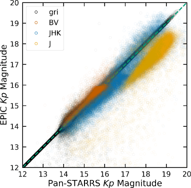
Figure 2: Comparison of $Kp$ magnitudes computed using Pan-STARRS $g$, $r$, and $i$-band photometry to previous measurements with optical (gri, black; BV, red) and infrared (JHK, blue; J, orange) photometry. Optical magnitude estimates are very similar. Previous measurements of $Kp$ from JHK photometry are skewed toward overestimating brightness. Previous $J$-band $Kp$ magnitude estimates are on average one magnitude brighter than our new optical measurements. The apparent truncation of Pan-STARRS $Kp$ measurements brighter than $\sim$14th magnitude for targets with previous estimates from BV, JHK, and $J$-band photometry is due to the Pan-STARRS saturation limit of $g\lesssim 14.5$. For targets with Pan-STARRS measurements brighter than the saturation limit, we instead used EPIC gri photometry when available. We truncate the plot at 12th magnitude to highlight computed $Kp$ differences, and because brighter targets follow the one-to-one line (gray dashed).

2.2 Gaia

Figure 3: $G-Kp$ versus K2/Gaia angular distance for single Gaia cross-match sources (upper left) and multiple Gaia cross-matches (upper right). For the sources with multiple cross-matches, we selected the target with the closest distance to the origin, which effectively removed the multiple cross-match cloud (lower left). For the final sample, we selected targets within $3\sigma$ of the average angular distance and $G-Kp$ (lower right).

We used the Gaia/K2 cross-match database to obtain distances to our K2 stars from Bailer-Jones et al. (2018). The 4″ radius cross-match between the aforementioned K2 observed star catalog and the Gaia DR2 catalog yields 361,488 Gaia/K2 entries and 294,114 unique EPIC IDs. We combined this cross-match table with our photometry table, reducing the Gaia/K2 cross-match sample to 256,990 Gaia sources within 4″ of our 275,153 K2 targets. The K2 targets without a Gaia cross-match are on average $\sim$2.5 magnitudes fainter ($Kp=16.38$) than those with a cross-match ($Kp=13.85$), and about 60% of these targets are likely giant stars (based on $J-K$ versus $r-J$ colors; Muirhead et al., 2015).

The similarities between the Gaia $G$-band ($\gtrsim 20\%$ transmission 4000–9000 Å; Evans et al., 2018) and Kepler $Kp$-band helped us to identify our K2 target in the Gaia data in the case of multiple cross-matches, which could be a binary companion or background source. There are 212,376 K2 targets with a single Gaia cross-match within 4″, 21,075 K2 targets with more than one cross-match, and 41,702 without any Gaia matches. There are a total of 44,614 different Gaia IDs for the 21,075 K2 targets with more than one cross-match.

We plot $G-Kp$ versus K2/Gaia angular distance in Figure 3 for both single and multiple cross-matches. If there were multiple cross-matches, we selected the target closest to the origin in $G-Kp$ and angular distance space (21,075 targets). For the multiple cross-matches, the distribution roughly follows that of single cross-match targets, but with a distinct branch extending into a cloud of sources with $G-Kp\gtrsim 0$ and angular distance $\gtrsim 0\farcs 75$. A simple investigation of targets along the extra branch in the closest Gaia cross-match plot does not indicate that these stars are distinct from the other closest match stars (e.g. common proper motion binary versus background star). Further analysis of this feature is encouraged but is beyond the scope of this work. For quality control, we selected targets from the single and closest Gaia cross-match lists within $3\sigma$ of the average angular distance ($\sim$1″) and $|G-Kp|$ ($\sim$1), leaving 231,761 unique targets (Figure 1).

2.3 LAMOST Spectra

LAMOST has a 4,000 fiber multi-object spectrograph (3690–9100 Å, $R\approx 1,800$) to survey stars and galaxies in the northern hemisphere (Cui et al., 2012). LAMOST DR5 v3 contains over nine million spectra. The LAMOST DR5 AFGK type star catalog is comprised of 5,348,712 spectra across all evolutionary stages, and the M dwarf catalog contains 534,393 spectra. We chose to use only LAMOST spectra because it contains more spectra than either APOGEE or RAVE. This also mitigated any effects from cross-calibrating spectroscopic parameters from other surveys.

We selected AFGK spectra with signal-to-noise (S/N) $>50$ in $g$ and $r$ bands, and M spectra with S/N $>50$ in $r$ and $i$ bands. Additionally, for comparison to our K2 catalog, we required that the LAMOST targets also have associated $g$, $r$, and $i$ band photometry. Thousands of targets, as identified by their 2MASS designation, were observed more than once, in which case we kept the target with the highest S/N in the $r$ band. This left us with 1,440,423 AFGK and 50,158 M star spectra with a unique 2MASS designation.

We used the Centre de Données astronomiques de Strasbourg (CDS) cross-match service to cross-match our Gaia/K2 and LAMOST catalogs using a 4″ search radius, yielding 29,134 AFGK and 1,737 M star matches. To ensure we matched the correct target, we checked that the absolute difference between $g$, $r$, and $i$ magnitudes in the LAMOST and EPIC catalogs were less than 0.15, a conservative $2\sigma$ from the median difference in each band. This left us with 25,450 AFGK and 1,388 M stars that are K2 targets with a LAMOST spectrum and Gaia parallax (Figure 1). For these targets, we computed absolute magnitudes for the $g,r,i,J,H,$ and $K_{s}$ band photometry from the EPIC catalog (Table 1), accounting for interstellar extinction using dustmaps (Green et al., 2018).

The LAMOST pipeline (Luo et al., 2012, 2015) assigns a Morgan-Keenan spectral type to each spectrum. For the AFGK catalog, $T_{\mathrm{eff}}$, $\log g$, and [Fe/H] were determined from the LAMOST stellar parameters pipeline (Wu et al., 2011), which uses the University of Lyon Spectroscopic analysis Software (ULySS) spectrum fitting package (Koleva et al., 2009). For M dwarfs, spectral type and atomic and molecular line indices were determined using The Hammer (Covey et al., 2007), but other stellar parameters were not derived (Yi et al., 2014). We discuss derivation of stellar radii and masses for AFGK stars in Section 3. In Section 4 we compute $T_{\mathrm{eff}}$, $\log g$, [Fe/H], $R_{\star}$, and $M_{\star}$ for M dwarfs.

3 AFGK Stellar Parameters

Since the LAMOST pipeline provides $T_{\mathrm{eff}}$, $\log g$, and [Fe/H] for AFGK stars, we can readily compute stellar radii in a similar fashion to Fulton & Petigura (2018). We first computed bolometric magnitudes ($M_{\mathrm{bol}}$) from $K_{s}$ band measurements, since $K_{s}$ is less affected by interstellar extinction than the other optical and near-infrared photometric bands:

$$M_{\mathrm{bol}}=m_{K_{s}}-5[\log_{10}(d)-1]-A_{K_{s}}-BC,$$ (2)

where $d$ is the distance computed from Gaia parallax measurements (Bailer-Jones et al., 2018), $A_{K_{s}}$ is the $K_{s}$ band interstellar extinction computed using dustmaps (Green et al., 2018), and BC is the bolometric correction. Bolometric corrections were computed using isoclassify, which interpolates the Modules for Experiments in Stellar Astrophysics (MESA) Isochrones and Stellar Tracks (MIST) grid (Dotter, 2016) over $T_{\mathrm{eff}}$, $\log g$, [Fe/H], and $A_{K_{s}}$. Bolometric luminosity ($L_{\mathrm{bol}}$) was calculated from bolometric magnitudes using:

$$L_{\mathrm{bol}}=L_{0}10^{-0.4M_{\mathrm{bol}}},$$ (3)

where $L_{0}\equiv 3.0128\times 10^{28}\,\mathrm{W}$ (Mamajek et al., 2015). Finally, we computed $R_{\star}$ from the Stefan-Boltzmann law:

$$R_{\star}=\left(\frac{L_{\mathrm{bol}}}{4\pi\sigma_{\mathrm{SB}}T_{\mathrm{eff}}^{4}}\right)^{1/2},$$ (4)

where $\sigma_{\mathrm{SB}}$ is the Stefan-Boltzmann constant. Since we have both $R_{\star}$ and $\log g$ measurements, $M_{\star}$ was computed using $M_{\star}=10^{\log g}\times R_{\star}^{2}/G$, where $G$ is the gravitational constant.

Uncertainties for parameters in this paper were computed using a Monte Carlo approach. For targets with symmetric uncertainties, we drew $10^{4}$ samples from a Gaussian distribution for each measured value and associated uncertainty. For targets with asymmetric uncertainties we drew $10^{4}$ samples from a split normal distribution, combining the left and right sides of two Gaussian distributions centered on the measured value and the negative and positive uncertainties. We propagated these distributions through each equation and took the median of the resultant distribution as the measured value and the 15.87 and 84.13 percentiles as the uncertainties. The average uncertainties on $R_{\star}$ and $M_{\star}$ for AFGK stars with LAMOST spectra are 4.4% and 14.9%, respectively. The very low uncertainties on these measurements are due to the $\sim$1% uncertainties on $T_{\mathrm{eff}}$ and $\log\,g$ provided by the LAMOST pipeline for high S/N targets.

4 M Dwarf Parameters

4.1 Spectral Type

The LAMOST data do not include $T_{\mathrm{eff}}$, $\log g$, and [Fe/H] for M dwarfs, so we derived our own parameters for these stars. M dwarfs in the LAMOST catalog were initially classified using a modified version of The Hammer (Covey et al., 2007), then they were visually inspected, which changed the classification of nearly 1/5 of the stars (Yi et al., 2014). Since visual inspection can introduce bias, we re-spectral typed our LAMOST M dwarfs in a uniform automated process using the spectral templates of Kesseli et al. (2017). These templates were derived from thousands of SDSS Baryon Oscillation Spectroscopic Survey (BOSS) spectra, covering 3600–10400 Å at a resolution of $R\approx 2,000$ (Dawson et al., 2013). We used the K5 to M7 dwarf templates, which are separated into 0.5 dex metallicity bins. We resampled the template spectra to match the resolution of the LAMOST spectra using SpectRes (Carnall, 2017). To identify the closest matching spectral template, we minimize the goodness-of-fit statistic $G_{K}$ (Equation 1 of Cushing et al., 2008), which is similar to $\chi^{2}$ minimization. In order to identify regions where the templates poorly fit our spectra, we ran the spectrum matching twice. First, using the same methods described in Section 5.1 of Mann et al. (2013b), we computed the residuals from the best-fit spectral template for each of the LAMOST spectra, then computed the median fractional deviation between the data and the templates at each wavelength. Regions with a median deviation greater than 10% were given a weight of 0 in $G_{K}$ for the second round of spectrum matching. This applied to $\lambda<5910\,\textrm{\AA}$, $7580\,\textrm{\AA}<\lambda<7660\,\textrm{\AA}$, and $\lambda>8800\,\textrm{\AA}$. The poor fit at blue wavelengths might be due to the nature of the LAMOST spectra, which are taken in two different channels (3700–5900 Å and 5700–9000 Å; Cui et al., 2012) and combined during processing. Spectral typing of M dwarfs has historically been done at red wavelengths (e.g., Kirkpatrick et al., 1991), so we made no additional attempt to fit the red and blue regions separately. In the top panel of Figure 4 we show an example M dwarf spectrum compared to its closest matching spectral template, with prominent atomic lines (H$\mathrm{\alpha}$, K I, Na I, Ca II) and molecular indices (CaH2, CaH3, TiO5) identified. In Figure 5, we compare our spectral types to those from the LAMOST pipeline for the same targets. Our classifications are more evenly distributed among the early M types with a peak near M1, whereas the LAMOST spectral types are significantly skewed toward M0. About 97% of our targets are within one spectral type of the LAMOST classification. We also identified a few late K dwarf interlopers that were assigned an M spectral type by LAMOST. We derived parameters for these K dwarfs in the same manner as our spectroscopic M dwarfs described below.

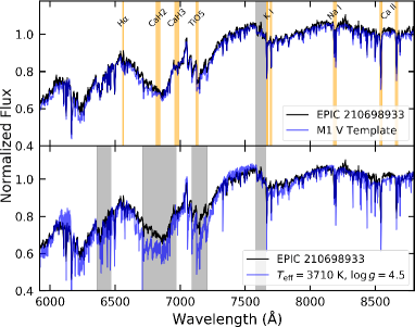
Figure 4: (Top) LAMOST spectrum of EPIC 210698933 (black) compared to an M1 V spectral template from Kesseli et al. (2017) (blue). A few prominent M dwarf atomic lines and molecular indices are indicated by the orange regions. (Bottom) The same spectrum compared to the closest matching PHOENIX-ACES model. Regions that the templates or models poorly matched the LAMOST spectra were masked out in the fitting process, which we show here in gray.

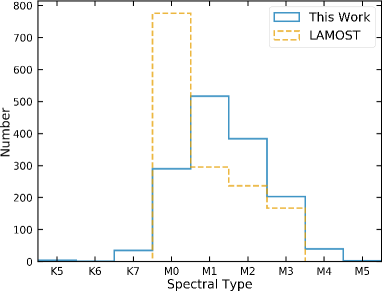
Figure 5: Comparison of spectral type classifications between LAMOST (dashed) and our pipeline (solid).

4.2 Effective Temperatures

We compared the LAMOST spectra to the PHOENIX-ACES model grid from Husser et al. (2013), which were sampled in increments of $T_{\mathrm{eff}}=100\,\mathrm{K}$, $\log g=0.5$, and $\mathrm{[Fe/H]}=0.5$. From these model spectra, we interpolated a finer model grid to $T_{\mathrm{eff}}=10\,\mathrm{K}$ and $\log g=0.1$, using $\mathrm{[Fe/H]}=0$ models. To identify the closest matching model spectrum, we used the same procedure outlined in Section 4.1, this time masking out the following regions: $\lambda<5920\,\textrm{\AA}$, $6360\,\textrm{\AA}<\lambda<6470\,\textrm{\AA}$, $6710\,\textrm{\AA}<\lambda<6970\,\textrm{\AA}$, $7090\,\textrm{\AA}<\lambda<7210\,\textrm{\AA}$, $7580\,\textrm{\AA}<\lambda<7660\,\textrm{\AA}$, and $\lambda>8800\,\textrm{\AA}$. In the bottom panel of Figure 4, we show the example spectrum compared to its closest matching spectral model, indicating regions that were masked out due to poor model fits. We adopt the temperatures from the closest matching spectral model but we refine our surface gravity measurements in Section 4.4.

Terrien et al. (2015) conducted a near-infrared spectroscopic survey of 886 nearby M dwarfs, from which they identified spectral types and measured temperatures and metallicities. From this list, we found a matching LAMOST spectrum for 108 targets that match our criteria above, which allows us to compare results from our methods. Terrien et al. (2015) identified spectral types using a spectroscopic $\mathrm{H}_{2}\mathrm{O}$–K2 index typing method first used by Rojas-Ayala et al. (2012) and updated by Newton et al. (2014). Our spectral types are on average a spectral type earlier than Terrien et al. (2015), which is illustrated in Figure 6a. For consistency with the spectral typing of earlier-type stars, we recommend using spectral types based on optical spectra rather than infrared spectra when possible. Effective temperatures in Terrien et al. (2015) were measured using $K_{s}$ band index calibrations from Mann et al. (2013b), which are valid in the range $3300\,\mathrm{K}<T_{\mathrm{eff}}<4800\,\mathrm{K}$. We compared our derived temperatures in Figure 6b, which shows the sharp temperature cutoff in the Terrien et al. (2015) data at 3300 K. Our temperatures are on average 20 K less than those of Terrien et al. (2015). Due to the similarity between temperature scales, we adopt the RMS scatter of 93 K for our $T_{\mathrm{eff}}$ uncertainties.

Figure 6: (a) Comparison of infrared spectral types from Terrien et al. (2015) to our optical spectral types from LAMOST spectra. The optical spectral types are on average a half spectral type earlier than those from infrared spectra. (b) Effective temperatures from infrared and optical spectra are similar, however, the infrared spectra temperature relationships used in Terrien et al. (2015) are only valid down to a range of 3300 K, which explains the sharp cut-off in the plot.

Figure 7: Color-magnitude diagrams colored by [Fe/H] for the Terrien et al. (2015) M dwarf sample (a) and our LAMOST FGK targets (b). The results for the LAMOST M dwarf [Fe/H] classification are shown in (c), and these results are combined with (a) and (b) in panel (d).

4.3 Metallicity

The myriad molecular lines at optical wavelengths hinder the measurement of metallicity from moderate resolution optical spectra. Metallicity for M dwarfs can be directly measured if they have a wide-separation F, G, or K dwarf primary companion, assuming the stars formed at the same time from the same molecular cloud (Bonfils et al., 2005). These stars allow the calibration of absolute photometric (e.g., Bonfils et al., 2005; Johnson & Apps, 2009; Schlaufman & Laughlin, 2010; Neves et al., 2012) and moderate resolution spectroscopic (e.g., Rojas-Ayala et al., 2010; Terrien et al., 2012; Rojas-Ayala et al., 2012; Mann et al., 2013a; Newton et al., 2014; Mann et al., 2014) methods. From moderate resolution optical spectra, the $\zeta$ parameter, computed from TiO and CaH spectroscopic indices, has shown a weak correlation with metallicity (e.g., Woolf et al., 2009; Mann et al., 2013a), and the LAMOST pipeline provides measurements of $\zeta$ for M dwarfs. Mann et al. (2013a) compared different methods for computing M dwarf metallicities, and found that the highest quality calibrations come from $K$ band features from moderate resolution infrared spectra.

Figure 8: (a) Comparison of predicted versus measured [Fe/H] from our random forest regression using only $M_{K_{s}}$ and $M_{g}-M_{K_{s}}$ and (b) using $M_{g}-M_{r}$, $M_{r}-M_{i}$, $M_{i}-M_{J}$, $M_{J}-M_{H}$, and $M_{H}-M_{K_{s}}$, which yields a tighter correlation. The 1:1 lines are plotted for reference.

We initially tried to use the spectral indices and $\zeta$ measurements provided by the LAMOST pipeline to determine metallicity on the set of 108 stars with both a LAMOST spectrum and a $K$-band metallicity measurement from Terrien et al. (2015), but we could not find any strong correlations. Instead, we calibrated a photometric metallicity relationship using 636 M dwarfs from Terrien et al. (2015) that have metallicity measurements, Gaia parallaxes, and $g$, $r$, $i$, $J$, $H$, and $K_{s}$-band photometry. We first computed absolute magnitudes for these targets. In Figure 7a, we plot $M_{K_{s}}$ versus $M_{g}-M_{K_{s}}$, with color indicating measured [Fe/H]. In this color space, there appears to be a metallicity gradient for M dwarfs, with larger $M_{g}-M_{K_{s}}$ colors generally indicating higher metallicity for the same $M_{K_{s}}$ magnitude. Due to the paucity of Terrien et al. (2015) targets with $M_{g}-M_{K_{s}}<5$, we also included 1,483 of our LAMOST AFGK targets with measured metallicities, $M_{K_{s}}>3$, and $M_{g}-M_{K_{s}}>3$ (Figure 7b). We trained a random forest regressor (scikit-learn; Pedregosa et al., 2011) with 1,000 trees on $M_{K_{s}}$ and $M_{g}-M_{K_{s}}$ for a random subset of 75% of the 2,119 targets with measured metallicities. We used the remaining 25% of targets to determine how well the regressor performed. Figure 8a compares the measured [Fe/H] to the predicted [Fe/H] from the random forest regressor. The median RMS scatter from 1,000 different random forest regressions using only $M_{K_{s}}$ and $M_{g}-M_{K_{s}}$ is 0.19. When we also included $M_{g}-M_{r}$, $M_{r}-M_{i}$, $M_{i}-M_{J}$, $M_{J}-M_{H}$, and $M_{H}-M_{K_{s}}$ as input parameters in the random forest regression, the median RMS scatter reduced to 0.17 (Figure 8b), which we took as the uncertainty in our M star [Fe/H] measurements. We plot the results from the [Fe/H] regression in Figure 7c and d.

4.4 Radius, Mass, and Surface Gravity

Mann et al. (2015) and Mann et al. (2019) derived empirical $M_{K_{s}}$–$R_{\star}$ and $M_{K_{s}}$–$M_{\star}$ relationships for M dwarfs to a precision below 3%. We used these relationships to compute radii and masses of our M dwarfs. We added the model uncertainties from Mann et al. (2015) and Mann et al. (2019) in quadrature to our calculated Monte Carlo uncertainties, yielding average radius and mass uncertainties of 3.1% and 6.6%, respectively. From mass and radius, we calculated surface gravity for these stars using $\log\,g=\log(GM_{\star}/R_{\star}^{2})$. We list all spectroscopically derived stellar parameters for AFGK and M stars in Table 1 and show a Hertzsprung-Russell (HR) diagram of all LAMOST targets in Figure 9.

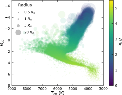
Figure 9: HR diagram LAMOST targets. Colors indicate surface gravity, and the size of the points represent stellar radius.

5 Photometric Classifcation

Using the 26,838 K2 targets classified from LAMOST spectra and Gaia parallaxes, we then classified stars with only photometry and Gaia parallaxes. The first step was to compute absolute magnitudes and the following colors to use for classification: $M_{g}-M_{K_{s}}$, $M_{g}-M_{r}$, $M_{r}-M_{i}$, $M_{i}-M_{J}$, $M_{J}-M_{H}$, and $M_{H}-M_{K_{s}}$. We first restricted our sample to K2 stars with these colors within the range of the LAMOST targets. This is necessary because random forest classification and regression cannot extrapolate beyond the range of the training set. This removed 9,673 targets from our sample, leaving us with 195,250 non-spectroscopic targets, and a total sample of 222,088 targets. A majority of the targets that were removed are fainter than $Kp=18$ (Figure 1).

We began classification with spectral types. Table 2 shows the number of targets with each spectral type in our LAMOST sample. Due to the relatively small numbers of A-type stars, we grouped A1-A6 stars into A5, and A8-A9 into A9 to increase the numbers in each respective bin for classification. In order to minimize bias due to different sample sizes, we randomly selected 100 stars from each spectral type to use for classification. For A5, A9, K2, and M4, we randomly sampled with replacement. In a similar manner to Section 4.3, we used these aforementioned colors along with $M_{K_{s}}$ to train a random forest classifier (scikit-learn; Pedregosa et al., 2011) with 1,000 trees on a random subset of 75% of the spectroscopic target subsample. The remaining 25% of the subsample were used to check the classifier performance. Figure 10 shows the measured versus predicted spectral type from the testing set. A majority of the predicted classifications are along or near the diagonal, indicating the classifier does a reasonable job at predicting spectral type. We used the trained classifier on all the photometric targets to yield spectral types. The assigned spectral types from photometry should be adequate for large statistical studies of K2 targets, but we caution their use for individual targets, and strongly encourage obtaining a spectrum for accurate spectral typing.

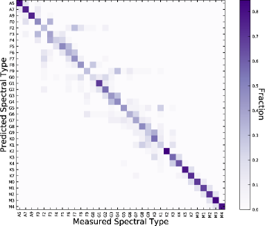
Figure 10: Measured versus predicted spectral types from our random forest classification, showing a reasonable prediction for most targets.

For effective temperature, surface gravity, and metallicity, we followed the same procedure outlined in Section 4.3, training a random forest regressor on $M_{K_{s}}$, $M_{g}-M_{K_{s}}$, $M_{g}-M_{r}$, $M_{r}-M_{i}$, $M_{i}-M_{J}$, $M_{J}-M_{H}$, and $M_{H}-M_{K_{s}}$ for our targets with spectroscopic $T_{\mathrm{eff}}$, $\log\,g$, and [Fe/H] measurements. Figure 11 shows the results from the testing set, with good fits for $T_{\mathrm{eff}}$ and $\log\,g$, and a positive correlation for [Fe/H]. We adopted the RMS scatter as the uncertainties for photometrically classified targets, which are 138 K, 0.15 dex, and 0.20 dex for $T_{\mathrm{eff}}$, $\log\,g$, and [Fe/H], respectively. Stellar radii and masses were then computed using the same procedures outlined in Section 3 for AFGK stars, and Section 4.4 for M stars. Average uncertainties on $R_{\star}$ and $M_{\star}$ for photometrically classified targets are 7% and 38%, respectively. We list the parameters for stars classified using photometry in Table 1.

Figure 11: Comparison of predicted versus measured $T_{\mathrm{eff}}$ (a), $\log\,g$ (b), and [Fe/H] (c) from our random forest regression using $M_{K_{s}}$, $M_{g}-M_{K_{s}}$, $M_{g}-M_{r}$, $M_{r}-M_{i}$, $M_{i}-M_{J}$, $M_{J}-M_{H}$, and $M_{H}-M_{K_{s}}$. The 1:1 lines are plotted for reference. There are tight correlations for $T_{\mathrm{eff}}$ and $\log\,g$, and a positive correlation for [Fe/H].

6 Discussion

6.1 Comparison to previous stellar measurements

The EPIC contains $T_{\mathrm{eff}}$, $\log\,g$, [Fe/H], $R_{\star}$, and $M_{\star}$ measurements for 192,598 of our targets, which allowed us to compare results. A significant fraction of the stellar properties for these targets in the EPIC were measured using reduced proper motions and colors (165,641), with LAMOST spectra accounting for 8,115 targets, RAVE spectra: 4,938 targets, APOGEE spectra: 1,413 targets, Hipparcos parallax: 4,912 targets, and colors only: 7,579 targets. In Figures 12, 13, and 14 we compare our $T_{\mathrm{eff}}$, $\log\,g$, [Fe/H], $R_{\star}$, and $M_{\star}$ measurements to those from the EPIC, delineating between the different EPIC classification inputs to see if there are any major trends depending on classification method. In general, our effective temperatures are similar regardless of classification method. For surface gravity there is much more structure, with a few preferential ‘arms’ appearing where there are significant interchanges between dwarfs and giants. There is a positive correlation between the measurements of [Fe/H], but in general our measurements appear to be larger. In the $R_{\star}$ comparisons, the giant-dwarf interchange arms are again apparent in the reduced proper motion and colors only plots. There are positive correlations between the mass measurements, but our mass measurements are generally larger than EPIC values.

The parameters derived from LAMOST spectra measurements are unsurprisingly similar, with deviations from unity mostly caused by our measurements of M dwarf properties. It is worth noting that our LAMOST measurements are from DR5, whereas the EPIC values come from LAMOST DR1. LAMOST pipeline updates changed computed parameters, and a comparison between LAMOST DR5 and DR3 for the same targets showed a standard deviation of 83 K, 0.13 dex, and 0.07 dex for $T_{\mathrm{eff}}$, $\log\,g$, and [Fe/H], respectively.

Using our $M_{K_{s}}$ values, we compare HR diagrams for $T_{\mathrm{eff}}$ in the EPIC and our values in Figure 15, showing additional information from surface gravities and radii. The aforementioned giant–dwarf misclassifications are clearly visible in the EPIC HR diagram.

Since there were no M giants in our LAMOST sample, it is difficult to accurately classify these targets for K2. M giants will have similar colors to M dwarfs, but very different luminosities. Table 1 contains a few hundred low surface gravity targets ($1.2\lesssim\log\,g\lesssim 3.9$) with an assigned M spectral type. Notably, these targets have temperatures higher than $\sim$4200 K, likely due to the random forest regressor assigning temperatures of nearby K giants with similar $M_{K_{s}}$ magnitudes. We urge caution when using our catalog parameters for targets toward the tip of the giant branch, and recommend using surface gravity and absolute magnitudes to help differentiate between main sequence and evolved stars.

Gaia measured $T_{\mathrm{eff}}$ and $R_{\star}$ for 174,781 of our stars, which we compare in Figure 16. The Gaia temperatures were estimated using $G$, $G_{BP}$, and $G_{RP}$ colors using a random forest algorithm trained on stars with $T_{\mathrm{eff}}$ determined from spectra (Andrae et al., 2018). In general, our $T_{\mathrm{eff}}$ measurements are comparable to Gaia measurements, but there appear to be more preferential temperatures in the Gaia targets, likely caused by their input training set. Our stellar radii correlate well with those determined from Gaia  which were measured in a similar manner to ours from the Stefan-Boltzmann law, using $M_{G}$ instead of $M_{K_{s}}$. Notably absent from Gaia measured radii are stars below $0.5\ R_{\odot}$.

Figure 12: Comparison of our temperature (a) and surface gravity (b) measurements to those from the EPIC. Each panel compares our measurements to the different methods used to derive the parameters in the EPIC, which allows us to elucidate any potential trends based on classification method.

Figure 13: Same as Figure 12, but for metallicity (a) and stellar radii (b).

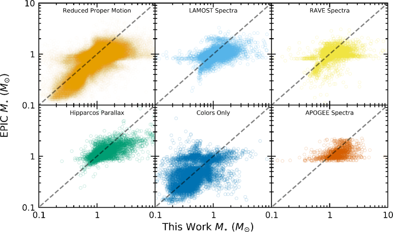
Figure 14: Same as Figure 12, but for stellar mass.

Figure 15: HR diagrams for (a) EPIC parameters and (b) our parameters. Colors indicate surface gravity, and the size of the points represent stellar radius. Several giant-dwarf interlopers are clearly visible in the EPIC HR diagram.

Figure 16: Comparison of our temperature (a) and stellar radius (b) measurements to those from Gaia. We caution readers to be careful when using Gaia effective temperatures. It is also notable that Gaia does not contain radius measurements for most M dwarfs smaller than $0.5\,R_{\odot}$.

Figure 17: Comparison of literature stellar radii (a) and planet radii (b) versus our measurements for confirmed and candidate hosts. Our radii for stars smaller than the Sun are typically larger than the values in the literature.

6.2 K2 planet hosts and the planet radius valley

We also compared $R_{\star}$ measurements for candidate and confirmed planet hosts, using the most recent measurements from the literature for targets with previously measured $R_{\star}$ and $R_{p}/R_{\star}$ (Figure 17a). This yielded parameters for 517 candidate and 299 confirmed planets and their hosts for which we also had an $R_{\star}$ measurement. We do not have new parameters for 375 candidates and 93 confirmed planets, which is due to either lack of previously measured $R_{\star}$ and $R_{p}/R_{\star}$ from the literature, lack of Gaia parallaxes, or the planet hosts do not fall within the color space necessary for our classification. For stars with radii less than $5\,R_{\odot}$, our $R_{\star}$ measurements are on average 8.6% and 7.9% larger than literature values for candidate and confirmed planet hosts, respectively. Looking specifically at M dwarfs with radii less than $0.6\,R_{\odot}$, our measurements are on average 18.5% and 33.3% larger for candidate and confirmed planet hosts. We attribute this significant discrepancy to previous measurements of M dwarf properties using older models which tend to underestimate the radii of cool stars. Using similar measurement techniques, Hardegree-Ullman et al. (2019) and Dressing et al. (2019) also noted that catalog radii for Kepler and K2 M dwarfs were underestimated by $\sim$40–50%.

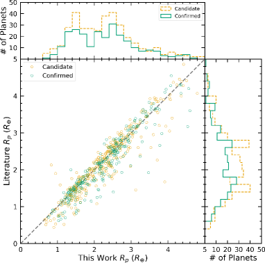
Figure 18: A closer inspection of planets with $R_{p}<5\,R_{\oplus}$ from Figure 17b elucidates a planet radius valley around $R_{p}\approx 1.9\,R_{\oplus}$ using our updated stellar parameters, which was not present in the previously measured planet radii.

For proper planet radius measurements, our new stellar properties should be used when fitting the transit light curves to account for effects such as limb darkening on the transit fit. Refitting transit curves is beyond the scope of this paper, but we offer a general quantitative analysis of updated planet radii $R_{p}$ based on literature values for $R_{p}/R_{\star}$ and our measurements of $R_{\star}$, which is valid under the assumption that the change of stellar parameters does not significantly affect the measured transit depth. Table Scaling K2. I. Revised Parameters for 222,088 K2 Stars and a K2 Planet Radius Valley at 1.9 $R_{\oplus}$ contains our revised planet radii, and Figure 17b compares our planet radii to literature values. For planets with $R_{p}<20\,R_{\oplus}$, our planet radii are on average 6.7% and 6.8% larger for candidate and confirmed planets, respectively.

Taking a closer look at planets with $R_{p}<5\,R_{\oplus}$, we investigated the planet radius valley, which is not apparent from previous K2 planet radii, but is very prominent in our revised radii (Figure 18). The Kruse et al. (2019) measurements constitute about 85% of the previous planet sample, indicating that the differences between our measured stellar radii and the Gaia pipeline are not insignificant, and likely due to the differences in $T_{\mathrm{eff}}$. We combined the confirmed and candidate K2 planet samples, and compared the planet radius distributions from our measurements to the Kepler sample from Fulton & Petigura (2018) and all previous K2 measurements for planets with orbital periods less than 80 days in Figure 19. Our updated stellar and planet radii confirm a distinct planet radius valley with a planet sample other than Kepler. This highlights the importance of careful and precise stellar measurements when deriving planet parameters. These measurements were not corrected for completeness, however, which is beyond the scope of this work. Completeness will be addressed in future catalog papers in this series (Zink et al. submitted, Zink et al. in preparation).

Figure 19: Normalized planet radius distributions for $R_{p}<5\,R_{\oplus}$ and $P<80$ days for our combined K2 confirmed and candidate sample to the Kepler sample from Fulton & Petigura (2018) (a), and all previous K2 measurements (b). There is a much more prominent valley in our measurements than in previous K2 measurements. The gap minimum around $R_{p}\approx 1.9\,R_{\oplus}$ that we measure is also consistent with the Kepler sample. Note, these measurements have not been corrected for completeness.

Using the literature values for orbital period and our computed stellar masses, we calculated semi-major axes $a$ for our set of K2 planets from Kepler’s third law. We then computed incident stellar flux $F_{pl}/F_{\oplus}=(L_{\star}/L_{\odot})(\mathrm{AU}/a)^{2}$, where stellar luminosity $L_{\star}/L_{\odot}=(R_{\star}/R_{\odot})^{2}(T_{\mathrm{eff}}/T_{\odot})^{4}$ computed using our values. In Figure 20 we show planet radius versus incident stellar flux for planets smaller than $4\,R_{\oplus}$ and orbital periods shorter than 80 days. The density contours show two relatively distinct populations of planets separated by a valley around $2\,R_{\oplus}$ and a wide range of incident fluxes. As a qualitative comparison, we also show the density contours of the K2 planet population and the Kepler population from Fulton & Petigura (2018). In both cases, the radius valley is apparent at about the same location, with hits of a small slope as a function of incident stellar flux.

Figure 20: (a) Planet radius versus incident stellar flux for K2 planets. Each point is either a confirmed or candidate planet, and the contours show the density of planets. A valley is present around $2\,R_{\oplus}$, separating a population of super-Earths and sub-Neptunes. (b) The same density contours for K2 from (a) with the density contours for Kepler planets from Fulton & Petigura (2018). The planet populations have similar distributions, with a similar radius gap showing a small slope with respect to incident stellar flux. Note that these plots have not been corrected for completeness.

Since we have spectral types for all of our stars, we separated the K2 planet radius distributions by spectral type (Figure 21). For each spectral type, there is a lack of planets at $R_{p}\approx 1.9\,R_{\oplus}$. K-type stars show a prominent radius valley, but all other spectral types at least hint at a valley. A larger sample size would be necessary to confirm a valley for F and M stars. Indeed, by combining 275 confirmed Kepler and 53 confirmed K2 K and M dwarf planets with host star $T_{\mathrm{eff}}<4,700\,\mathrm{K}$, Cloutier & Menou (2019) showed a more definitive planet valley around $1.54\,R_{\oplus}$ for planets around cool stars. Further, there is an increasing total fraction of super-Earths ($R_{\oplus}<R_{p}<1.9\,R_{\oplus}$) to sub-Neptunes ($1.9\,R_{\oplus}<R_{p}<3.86\,R_{\oplus}$) toward later-type stars, with ratios of 0.20, 0.50, 0.82, and 1.13 for F, G, K, and M stars, respectively, which is consistent with conclusions of planet occurrence rate studies (e.g., Howard et al., 2012; Dressing & Charbonneau, 2015; Mulders et al., 2015; Hardegree-Ullman et al., 2019), indicating that smaller planets are more common toward later spectral types. This effect, however, could be an observational bias, since it is more difficult to detect smaller planets around larger stars. We also compared the planet radius distributions for single and multiple planet systems in Figures 21 and 22. There are 602 single planet systems and 90 multiple planet systems containing a total of 214 planets. For single planet systems, the ratio of super-Earths to sub-Neptunes is 0.51, whereas for multiple planet systems the ratio is 1.02. We leave the analysis of these effects to future studies.

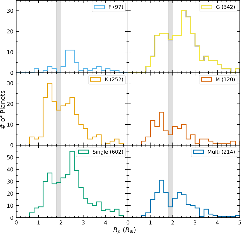
Figure 21: Planet radius distributions separated by spectral type, including both confirmed and candidate planets (top four panels), and single versus multiple planet systems (bottom two panels). We have shaded the region at $1.9\,R_{\oplus}$ for reference in comparison to the radius valley of the total sample. For each spectral type there is evidence for the planet radius valley, which is most prominent for K-type stars. Single planet systems appear to have about twice the fraction of sub-Neptunes compared to super-Earths, whereas the ratio is near unity for multiple planet systems. We again note that these distributions have not been corrected for completeness, so conclusions about planet occurrence rates cannot be drawn from these data.

Figure 22: Planet radius versus incident stellar flux for K2 planets in single (a) and multiple planet systems (b). Perhaps more evident than in Figure 21, single planet systems appear to have twice as many sub-Neptunes than super-Earths, whereas multiple planet systems have roughly equal numbers of each. Note that these plots have not been corrected for completeness.

6.3 Future directions

Our uniformly derived catalog of updated stellar parameters for 222,088 K2 stars using LAMOST spectra, Gaia parallaxes, and photometry is a crucial step in the process of calculating K2 planet occurrence rates. All of the planet candidates analyzed in this paper were from K2 Campaigns 1–13, since catalogs for those planets have already been made and are available on the Exoplanet Archive. The next step toward computing planet occurrence rates is to develop a pipeline to uniformly process K2 light curves and automatically identify and vet planet candidates across all campaigns (Zink et al. submitted, Zink et al. in preparation). This will enable us to conduct crucial completeness and reliability tests necessary for accurate planet occurrence rate calculations, and which we have not been able to account for in this work. With a larger set of planet candidates across all campaigns, a more complete analysis of effects such as the planet radius gap can be assessed. Our large set of $T_{\mathrm{eff}}$, $\log\,g$, [Fe/H], $R_{\star}$, and $M_{\star}$ can also enable other statistical population studies of stars and planets.

In this study we have largely ignored the effects of stellar multiplicity. Duchêne & Kraus (2013) estimate that 44% of all FGK stars are part of a multiple stellar system, and Winters et al. (2019) found a multiplicity rate of $\sim$27% for M dwarfs within 25 pc of the Sun. Gaia is able to resolve binary stars of similar brightness with separations down to about one arcsecond, however, Horch et al. (2014) estimate that 40-50% of planet candidate systems host a bound binary within one arcsecond. Our stellar parameters assume a single star or a wide separation such that we can resolve our target. If the stars are actually in multiple systems our stellar radii will typically be overestimated, which could have a significant impact on derived planet parameters and conclusions regarding planet populations (e.g., Ciardi et al., 2015; Furlan et al., 2017; Horch et al., 2017; Matson et al., 2018). High-resolution imaging surveys to determine stellar multiplicity rates have largely focused on stars with planet candidates, but it is possible that there are differences in multiplicity rates for hosts versus non-hosts, which could suggest differences in formation mechanisms. We strongly encourage additional high-resolution imaging and high-resolution spectroscopic observations of K2 stars, including stars without known planets, that enable us to more effectively mitigate and assess the impact of stellar companions on planet occurrence rates.

7 Acknowledgements

We thank the anonymous referee who provided several helpful suggestions that improved this manuscript. We would also like to thank Christina Hedges, Geert Barentsen, and Jessie Dotson at the Kepler Guest Observer office for constructive discussions about K2 and this work.

This research has made use of the NASA Exoplanet Archive, which is operated by the California Institute of Technology, under contract with the National Aeronautics and Space Administration under the Exoplanet Exploration Program.

The Pan-STARRS1 Surveys (PS1) and the PS1 public science archive have been made possible through contributions by the Institute for Astronomy, the University of Hawaii, the Pan-STARRS Project Office, the Max-Planck Society and its participating institutes, the Max Planck Institute for Astronomy, Heidelberg and the Max Planck Institute for Extraterrestrial Physics, Garching, The Johns Hopkins University, Durham University, the University of Edinburgh, the Queen’s University Belfast, the Harvard-Smithsonian Center for Astrophysics, the Las Cumbres Observatory Global Telescope Network Incorporated, the National Central University of Taiwan, the Space Telescope Science Institute, the National Aeronautics and Space Administration under Grant No. NNX08AR22G issued through the Planetary Science Division of the NASA Science Mission Directorate, the National Science Foundation Grant No. AST-1238877, the University of Maryland, Eotvos Lorand University (ELTE), the Los Alamos National Laboratory, and the Gordon and Betty Moore Foundation.

This work has made use of data from the European Space Agency (ESA) mission Gaia (https://www.cosmos.esa.int/gaia), processed by the Gaia Data Processing and Analysis Consortium (DPAC, https://www.cosmos.esa.int/web/gaia/dpac/consortium). Funding for the DPAC has been provided by national institutions, in particular the institutions participating in the Gaia Multilateral Agreement.

This work made use of the gaia-kepler.fun cross-match database created by Megan Bedell. This research made use of the cross-match service provided by CDS, Strasbourg.

Guoshoujing Telescope (the Large Sky Area Multi-Object Fiber Spectroscopic Telescope, LAMOST) is a National Major Scientific Project built by the Chinese Academy of Sciences. Funding for the project has been provided by the National Development and Reform Commission. LAMOST is operated and managed by the National Astronomical Observatories, Chinese Academy of Sciences.

K. H-U acknowledges funding from NASA ADAP grant 80NSSC18K0431.

Table 1: K2 stellar parameters.

EPIC ID	K2 Campaign	Pan-STARRS ID	Gaia DR2 ID	LAMOST ID	$m_{g}$	$\cdots$
					(mag)
201048855	10	$\cdots$	3582456140266586240	$\cdots$	$12.320\pm 0.040$
201049999	10	$\cdots$	3582457617736883840	$\cdots$	$13.353\pm 0.030$
201050049	10	$\cdots$	3582457858255051392	$\cdots$	$14.043\pm 0.040$
201050511	10	$\cdots$	3582458579809568256	$\cdots$	$11.405\pm 0.030$
201051317	10	98321820422274493	3582459163925111552	$\cdots$	$15.285\pm 0.003$
201051625	10	$\cdots$	3582459301364064768	$\cdots$	$12.821\pm 0.040$
201052484	10	$\cdots$	3582465176879327488	$\cdots$	$13.713\pm 0.050$
201054099	10	98441820384293565	3582468612853166080	$\cdots$	$15.090\pm 0.003$
201054338	10	$\cdots$	3582466619988381184	$\cdots$	$12.188\pm 0.050$
201054542	10	98461822154792184	3582466997945503616	$\cdots$	$14.871\pm 0.005$
201054991	10	98471821477879568	3582467582061055360	$\cdots$	$15.185\pm 0.003$
201071559	10	99101827692668111	3582605914368082816	$\cdots$	$16.649\pm 0.005$
201071583	10	99101826522918865	3582603406107179264	$\cdots$	$18.861\pm 0.014$
201071950	10	99121828753012622	3582605502051225216	$\cdots$	$14.848\pm 0.003$
201071997	10	99121826550054361	3582603440466918016	$\cdots$	$17.159\pm 0.004$
201072036	10	$\cdots$	3594613577775506048	$\cdots$	$15.455\pm 0.020$
201072674	10	99141828915398845	3582607220038146176	$\cdots$	$14.921\pm 0.002$
201073202	10	$\cdots$	3594613440336532224	$\cdots$	$15.761\pm 0.030$
201073315	10	99171829021981565	3582607323117362688	$\cdots$	$15.693\pm 0.060$
201073427	10	$\cdots$	3594616154755833984	$\cdots$	$14.027\pm 0.020$
201073453	10	$\cdots$	3594616253538685824	$\cdots$	$13.622\pm 0.040$
201073867	10	99191826959622285	3582610346774334336	$\cdots$	$17.607\pm 0.006$
201073911	10	99191829080563936	3582607421901033856	$\cdots$	$16.277\pm 0.006$
201074123	10	99201827274061451	3582610003176952320	$\cdots$	$17.683\pm 0.002$
201074212	10	$\cdots$	3582609865738000000	$\cdots$	$11.700\pm 0.030$
201074534	10	99211822135945395	3594605709395368832	$\cdots$	$15.479\pm 0.004$
201074673	10	$\cdots$	3594614608567639808	$\cdots$	$14.109\pm 0.020$
201074674	10	$\cdots$	3594605812474584704	$\cdots$	$12.950\pm 0.030$
201074775	10	$\cdots$	3582607834216399104	$\cdots$	$12.096\pm 0.030$
201074882	10	99221824760577057	3594618010181737088	$\cdots$	$14.993\pm 0.003$
201075355	10	99241827756634091	3582611652444397312	$\cdots$	$18.450\pm 0.007$
201075442	10	$\cdots$	3594606774547212160	$\cdots$	$12.263\pm 0.030$

Note. — This table is available in its entirety in machine-readable form online.

Note. — There are 222,088 unique targets in this table. There were 19,829 targets observed in two or three campaigns, which we list as separate entries for each K2 campaign. This table contains a total of 244,337 entries.

Note. — Apparent $g$, $r$, and $i$-band magnitudes are from Pan-STARRS for targets with a Pan-STARRS ID and from UCAC4 or SDSS as reported in the EPIC (Huber et al., 2016) otherwise.

Note. — Spectral type, $T_{\mathrm{eff}}$, $\log\,g$, and [Fe/H] for stars with a LAMOST ID were derived using LAMOST spectra. These parameters for stars without a LAMOST ID were derived using photometry trained on the spectroscopic sample.

Table 2: Number of targets in our LAMOST sample with each spectral type classification.

Type	#	Type	#	Type	#	Type	#
A1	6	F3	179	G3	2399	K3	682
A2	2	F4	131	G4	580	K4	280
A3	7	F5	1649	G5	4009	K5	457
A5	23	F6	639	G6	669	K7	245
A6	33	F7	1038	G7	1762	M0	278
A7	109	F8	276	G8	1266	M1	496
A8	10	F9	2122	G9	563	M2	377
A9	13	G0	915	K0	363	M3	195
F0	962	G1	328	K1	1155	M4	40
F2	703	G2	1861	K2	17	M5	2

Table 3: Refined K2 planet parameters.

EPIC ID	Candidate ID	Confirmed Planet Name	$R_{p}/R_{\star}$	Period	Reference	Spectral Type	$\cdots$
				(days)
201110617	201110617.01	K2-156 b	$0.01704^{+0.00139}_{-0.00114}$	$0.813149^{+0.000050}_{-0.000049}$	5	K5
201111557	201111557.01	$\cdots$	$0.01692^{+0.00674}_{-0.00148}$	$2.302368^{+0.000105}_{-0.000103}$	5	K3
201127519	201127519.01	$\cdots$	$0.11511^{+0.00492}_{-0.00336}$	$6.178369^{+0.000195}_{-0.000172}$	5	K3
201130233	201130233.01	K2-157 b	$0.01105^{+0.00143}_{-0.00097}$	$0.365257^{+0.000029}_{-0.000029}$	5	G7
201132684	201132684.01	K2-158 b	$0.02707^{+0.00275}_{-0.00198}$	$10.062106^{+0.00227}_{-0.002228}$	5	G7
201152065	201152065.01	$\cdots$	$0.0226^{+0.0022}_{-0.0055}$	$10.6966^{+0.002}_{-0.0021}$	3	K5
201155177	201155177.01	K2-42 b	$0.0313^{+0.0023}_{-0.0047}$	$6.68851^{+0.00074}_{-0.00075}$	3	K5
201160662	201160662.01	$\cdots$	$0.259^{+0.071}_{-0.099}$	$1.5374115^{+0.0000062}_{-0.0000061}$	3	F6
201166680	201166680.01	$\cdots$	$0.01572^{+0.00173}_{-0.00119}$	$18.10549^{+0.010083}_{-0.012897}$	5	F2
201176672	201176672.01	$\cdots$	$0.18^{+0.011}_{-0.011}$	$79.9999^{+0.0098}_{-0.0098}$	2	K5
201197348	201197348.01	$\cdots$	$0.046^{+0.0038}_{-0.0078}$	$14.9139^{+0.0018}_{-0.002}$	3	K5
201205469	201205469.01	K2-43 b	$0.0775^{+0.0034}_{-0.0063}$	$3.471136^{+0.000079}_{-0.000079}$	3	M1
201205469	201205469.02	K2-43 c	$0.0391^{+0.0039}_{-0.0113}$	$2.19945^{+0.00015}_{-0.00014}$	3	M1
201208431	201208431.01	K2-4 b	$0.0368^{+0.0015}_{-0.0031}$	$10.0051^{+0.00044}_{-0.00043}$	3	K7
201211526	201211526.01	K2-244 b	$0.01698^{+0.00312}_{-0.00127}$	$21.070201^{+0.002413}_{-0.002267}$	5	G3
201225286	201225286.01	K2-159 b	$0.02439^{+0.00226}_{-0.00134}$	$12.421078^{+0.001049}_{-0.001001}$	5	G7
201227197	201227197.01	K2-160 b	$0.03189^{+0.00171}_{-0.00114}$	$3.705871^{+0.000074}_{-0.000076}$	5	G4
201231064	201231064.01	K2-161 b	$0.02184^{+0.00518}_{-0.00181}$	$9.283188^{+0.002052}_{-0.0023}$	5	G5
201238110	201238110.01	$\cdots$	$0.0505^{+0.005}_{-0.0129}$	$7.90417^{+0.00091}_{-0.00148}$	3	M2
201238110	201238110.02	EPIC 201238110 b	$0.054^{+0.0034}_{-0.0054}$	$28.1696^{+0.0038}_{-0.0043}$	3	M2
201239401	201239401.01	$\cdots$	$0.025^{+0.0019}_{-0.0039}$	$0.905655^{+0.000049}_{-0.000050}$	3	M2
201247497	201247497.01	$\cdots$	$0.087^{+0.011}_{-0.07}$	$2.75421^{+0.00012}_{-0.00012}$	3	M0
201259803	201259803.01	$\cdots$	$0.1173^{+0.0034}_{-0.0035}$	$1.684208^{+0.000024}_{-0.000024}$	3	M1
201264302	201264302.01	$\cdots$	$0.0253^{+0.0018}_{-0.006}$	$0.2122013^{+0.0000023}_{-0.0000018}$	3	M3
201295312	201295312.01	K2-44 b	$0.01775^{+0.00066}_{-0.00165}$	$5.65621^{+0.00026}_{-0.00027}$	3	G0
201299088	201299088.01	$\cdots$	$0.04741^{+0.00197}_{-0.00184}$	$21.204739^{+0.005348}_{-0.005523}$	5	G8
201324549	201324549.01	$\cdots$	$0.089^{+0.022}_{-0.039}$	$2.519386^{+0.000014}_{-0.000014}$	3	F5
201338508	201338508.01	K2-5 c	$0.0348^{+0.0031}_{-0.0079}$	$10.93459^{+0.00088}_{-0.00105}$	3	K7
201338508	201338508.02	K2-5 b	$0.073^{+0.021}_{-0.039}$	$5.73649^{+0.00033}_{-0.00034}$	3	K7
201345483	201345483.01	K2-45 b	$0.1431^{+0.005}_{-0.0044}$	$1.7292577^{+0.0000049}_{-0.0000050}$	3	K5
201352100	201352100.01	$\cdots$	$0.03231^{+0.00186}_{-0.00145}$	$13.383629^{+0.00076}_{-0.000727}$	5	K1
201357835	201357835.01	$\cdots$	$0.03044^{+0.001}_{-0.00079}$	$11.8951^{+0.0014}_{-0.0017}$	7	F8
201359834	201359834.01	$\cdots$	$0.266^{+0.081}_{-0.128}$	$40.1401^{+0.0012}_{-0.0012}$	3	M1
201366540	201366540.01	$\cdots$	$0.0346^{+0.0054}_{-0.0295}$	$7.4433^{+0.0011}_{-0.0012}$	3	K7
201367065	201367065.01	K2-3 b	$0.0358^{+0.0012}_{-0.0031}$	$10.05467^{+0.00011}_{-0.00011}$	3	M1
201367065	201367065.02	K2-3 c	$0.0291^{+0.0027}_{-0.0027}$	$24.64671^{+0.00054}_{-0.00053}$	3	M1
201367065	201367065.03	K2-3 d	$0.0273^{+0.0029}_{-0.0048}$	$44.5574^{+0.0023}_{-0.0023}$	3	M1
201384232	201384232.01	K2-6 b	$0.0259^{+0.0013}_{-0.003}$	$30.9403^{+0.0023}_{-0.0027}$	3	G3
201390048	201390048.01	K2-162 b	$0.01878^{+0.00206}_{-0.00141}$	$9.457747^{+0.001401}_{-0.001392}$	5	K5
201393098	201393098.01	K2-7 b	$0.0247^{+0.0015}_{-0.0036}$	$28.6911^{+0.0037}_{-0.0042}$	3	G6
201403446	201403446.01	K2-46 b	$0.01764^{+0.00086}_{-0.0021}$	$19.153^{+0.002}_{-0.0022}$	3	F6
201427874	201427874.01	K2-163 b	$0.02966^{+0.00301}_{-0.0014}$	$6.673117^{+0.000316}_{-0.000303}$	5	K4
201437844	201437844.01	HD 106315 b	$0.01677^{+0.00101}_{-0.00067}$	$9.554515^{+0.001256}_{-0.001368}$	5	F4

: (1) Adams et al. (2016), (2) Crossfield et al. (2016), (3) Kruse et al. (2019), (4) Mann et al. (2017), (5) Mayo et al. (2018), (6) Osborn et al. (2016), (7) Zink et al. (2019).

Note. — This table is available in its entirety in machine-readable form online.

References. — References for $R_{p}/R_{\star}$ and Period

References

- Adams et al. (2016) Adams, E. R., Jackson, B., & Endl, M. 2016, AJ, 152, 47, doi: 10.3847/0004-6256/152/2/47
- Alam et al. (2015) Alam, S., Albareti, F. D., Allende Prieto, C., et al. 2015, ApJS, 219, 12, doi: 10.1088/0067-0049/219/1/12
- Andrae et al. (2018) Andrae, R., Fouesneau, M., Creevey, O., et al. 2018, A&A, 616, A8, doi: 10.1051/0004-6361/201732516
- Astropy Collaboration et al. (2013) Astropy Collaboration, Robitaille, T. P., Tollerud, E. J., et al. 2013, A&A, 558, A33, doi: 10.1051/0004-6361/201322068
- Astropy Collaboration et al. (2018) Astropy Collaboration, Price-Whelan, A. M., Sipőcz, B. M., et al. 2018, AJ, 156, 123, doi: 10.3847/1538-3881/aabc4f
- Bailer-Jones et al. (2018) Bailer-Jones, C. A. L., Rybizki, J., Fouesneau, M., Mantelet, G., & Andrae, R. 2018, AJ, 156, 58, doi: 10.3847/1538-3881/aacb21
- Berger et al. (2018) Berger, T. A., Huber, D., Gaidos, E., & van Saders, J. L. 2018, ApJ, 866, 99, doi: 10.3847/1538-4357/aada83
- Bonfils et al. (2005) Bonfils, X., Delfosse, X., Udry, S., et al. 2005, A&A, 442, 635, doi: 10.1051/0004-6361:20053046
- Borucki et al. (2010) Borucki, W. J., Koch, D., Basri, G., et al. 2010, Science, 327, 977, doi: 10.1126/science.1185402
- Boyajian et al. (2012) Boyajian, T. S., von Braun, K., van Belle, G., et al. 2012, ApJ, 757, 112, doi: 10.1088/0004-637X/757/2/112
- Brown et al. (2011) Brown, T. M., Latham, D. W., Everett, M. E., & Esquerdo, G. A. 2011, AJ, 142, 112, doi: 10.1088/0004-6256/142/4/112
- Carnall (2017) Carnall, A. C. 2017, arXiv e-prints, arXiv:1705.05165. https://arxiv.org/abs/1705.05165
- Chambers et al. (2016) Chambers, K. C., Magnier, E. A., Metcalfe, N., et al. 2016, arXiv e-prints, arXiv:1612.05560. https://arxiv.org/abs/1612.05560
- Ciardi et al. (2015) Ciardi, D. R., Beichman, C. A., Horch, E. P., & Howell, S. B. 2015, ApJ, 805, 16, doi: 10.1088/0004-637X/805/1/16
- Cloutier & Menou (2019) Cloutier, R., & Menou, K. 2019, arXiv e-prints, arXiv:1912.02170. https://arxiv.org/abs/1912.02170
- Covey et al. (2007) Covey, K. R., Ivezić, Ž., Schlegel, D., et al. 2007, AJ, 134, 2398, doi: 10.1086/522052
- Crossfield et al. (2016) Crossfield, I. J. M., Ciardi, D. R., Petigura, E. A., et al. 2016, ApJS, 226, 7, doi: 10.3847/0067-0049/226/1/7
- Cui et al. (2012) Cui, X.-Q., Zhao, Y.-H., Chu, Y.-Q., et al. 2012, Research in Astronomy and Astrophysics, 12, 1197, doi: 10.1088/1674-4527/12/9/003
- Cushing et al. (2008) Cushing, M. C., Marley, M. S., Saumon, D., et al. 2008, ApJ, 678, 1372, doi: 10.1086/526489
- Dawson et al. (2013) Dawson, K. S., Schlegel, D. J., Ahn, C. P., et al. 2013, AJ, 145, 10, doi: 10.1088/0004-6256/145/1/10
- Dotter (2016) Dotter, A. 2016, ApJS, 222, 8, doi: 10.3847/0067-0049/222/1/8
- Dressing & Charbonneau (2015) Dressing, C. D., & Charbonneau, D. 2015, ApJ, 807, 45, doi: 10.1088/0004-637X/807/1/45
- Dressing et al. (2017a) Dressing, C. D., Newton, E. R., Schlieder, J. E., et al. 2017a, ApJ, 836, 167, doi: 10.3847/1538-4357/836/2/167
- Dressing et al. (2017b) Dressing, C. D., Vanderburg, A., Schlieder, J. E., et al. 2017b, AJ, 154, 207, doi: 10.3847/1538-3881/aa89f2
- Dressing et al. (2019) Dressing, C. D., Hardegree-Ullman, K., Schlieder, J. E., et al. 2019, AJ, 158, 87, doi: 10.3847/1538-3881/ab2895
- Duchêne & Kraus (2013) Duchêne, G., & Kraus, A. 2013, ARA&A, 51, 269, doi: 10.1146/annurev-astro-081710-102602
- Evans et al. (2018) Evans, D. W., Riello, M., De Angeli, F., et al. 2018, A&A, 616, A4, doi: 10.1051/0004-6361/201832756
- Flewelling et al. (2016) Flewelling, H. A., Magnier, E. A., Chambers, K. C., et al. 2016, ArXiv e-prints. https://arxiv.org/abs/1612.05243
- Fulton & Petigura (2018) Fulton, B. J., & Petigura, E. A. 2018, AJ, 156, 264, doi: 10.3847/1538-3881/aae828
- Fulton et al. (2017) Fulton, B. J., Petigura, E. A., Howard, A. W., et al. 2017, AJ, 154, 109, doi: 10.3847/1538-3881/aa80eb
- Furlan et al. (2017) Furlan, E., Ciardi, D. R., Everett, M. E., et al. 2017, AJ, 153, 71, doi: 10.3847/1538-3881/153/2/71
- Gaia Collaboration et al. (2016) Gaia Collaboration, Prusti, T., de Bruijne, J. H. J., et al. 2016, A&A, 595, doi: 10.1051/0004-6361/201629272
- Gaia Collaboration et al. (2018) Gaia Collaboration, Brown, A. G. A., Vallenari, A., et al. 2018, A&A, 616, A1, doi: 10.1051/0004-6361/201833051
- Girardi et al. (2000) Girardi, L., Bressan, A., Bertelli, G., & Chiosi, C. 2000, A&AS, 141, 371, doi: 10.1051/aas:2000126
- Green et al. (2018) Green, G. M., Schlafly, E. F., Finkbeiner, D., et al. 2018, MNRAS, 478, 651, doi: 10.1093/mnras/sty1008
- Hardegree-Ullman et al. (2019) Hardegree-Ullman, K. K., Cushing, M. C., Muirhead, P. S., & Christiansen, J. L. 2019, AJ, 158, 75, doi: 10.3847/1538-3881/ab21d2
- Horch et al. (2014) Horch, E. P., Howell, S. B., Everett, M. E., & Ciardi, D. R. 2014, ApJ, 795, 60, doi: 10.1088/0004-637X/795/1/60
- Horch et al. (2017) Horch, E. P., Casetti-Dinescu, D. I., Camarata, M. A., et al. 2017, AJ, 153, 212, doi: 10.3847/1538-3881/aa6749
- Howard et al. (2012) Howard, A. W., Marcy, G. W., Bryson, S. T., et al. 2012, ApJS, 201, 15, doi: 10.1088/0067-0049/201/2/15
- Howell et al. (2012) Howell, S. B., Rowe, J. F., Bryson, S. T., et al. 2012, ApJ, 746, 123, doi: 10.1088/0004-637X/746/2/123
- Howell et al. (2014) Howell, S. B., Sobeck, C., Haas, M., et al. 2014, PASP, 126, 398, doi: 10.1086/676406
- Huber et al. (2016) Huber, D., Bryson, S. T., Haas, M. R., et al. 2016, The Astrophysical Journal Supplement Series, 224, 2, doi: 10.3847/0067-0049/224/1/2
- Hunter (2007) Hunter, J. D. 2007, Computing in Science & Engineering, 9, 90, doi: 10.1109/MCSE.2007.55
- Husser et al. (2013) Husser, T. O., Wende-von Berg, S., Dreizler, S., et al. 2013, A&A, 553, A6, doi: 10.1051/0004-6361/201219058
- Johnson & Apps (2009) Johnson, J. A., & Apps, K. 2009, ApJ, 699, 933, doi: 10.1088/0004-637X/699/2/933
- Jones et al. (2001) Jones, E., Oliphant, T., Peterson, P., et al. 2001, SciPy: Open source scientific tools for Python. http://www.scipy.org/
- Kesseli et al. (2017) Kesseli, A. Y., West, A. A., Veyette, M., et al. 2017, ApJS, 230, 16, doi: 10.3847/1538-4365/aa656d
- Kirkpatrick et al. (1991) Kirkpatrick, J. D., Henry, T. J., & McCarthy, Jr., D. W. 1991, ApJS, 77, 417, doi: 10.1086/191611
- Koleva et al. (2009) Koleva, M., Prugniel, P., Bouchard, A., & Wu, Y. 2009, A&A, 501, 1269, doi: 10.1051/0004-6361/200811467
- Kordopatis et al. (2013) Kordopatis, G., Gilmore, G., Steinmetz, M., et al. 2013, AJ, 146, 134, doi: 10.1088/0004-6256/146/5/134
- Kruse et al. (2019) Kruse, E., Agol, E., Luger, R., & Foreman-Mackey, D. 2019, ApJS, 244, 11, doi: 10.3847/1538-4365/ab346b
- Lee & Chiang (2016) Lee, E. J., & Chiang, E. 2016, ApJ, 817, 90, doi: 10.3847/0004-637X/817/2/90
- Lee et al. (2014) Lee, E. J., Chiang, E., & Ormel, C. W. 2014, ApJ, 797, 95, doi: 10.1088/0004-637X/797/2/95
- Lopez & Rice (2018) Lopez, E. D., & Rice, K. 2018, MNRAS, 479, 5303, doi: 10.1093/mnras/sty1707
- Luo et al. (2012) Luo, A. L., Zhang, H.-T., Zhao, Y.-H., et al. 2012, Research in Astronomy and Astrophysics, 12, 1243, doi: 10.1088/1674-4527/12/9/004
- Luo et al. (2015) Luo, A. L., Zhao, Y.-H., Zhao, G., et al. 2015, Research in Astronomy and Astrophysics, 15, 1095, doi: 10.1088/1674-4527/15/8/002
- Mamajek et al. (2015) Mamajek, E. E., Torres, G., Prsa, A., et al. 2015, ArXiv e-prints. https://arxiv.org/abs/1510.06262
- Mann et al. (2013a) Mann, A. W., Brewer, J. M., Gaidos, E., Lépine, S., & Hilton, E. J. 2013a, AJ, 145, 52, doi: 10.1088/0004-6256/145/2/52
- Mann et al. (2014) Mann, A. W., Deacon, N. R., Gaidos, E., et al. 2014, AJ, 147, 160, doi: 10.1088/0004-6256/147/6/160
- Mann et al. (2015) Mann, A. W., Feiden, G. A., Gaidos, E., Boyajian, T., & von Braun, K. 2015, ApJ, 804, 64, doi: 10.1088/0004-637X/804/1/64
- Mann et al. (2013b) Mann, A. W., Gaidos, E., & Ansdell, M. 2013b, ApJ, 779, 188, doi: 10.1088/0004-637X/779/2/188
- Mann et al. (2017) Mann, A. W., Gaidos, E., Vanderburg, A., et al. 2017, AJ, 153, 64, doi: 10.1088/1361-6528/aa5276
- Mann et al. (2019) Mann, A. W., Dupuy, T., Kraus, A. L., et al. 2019, ApJ, 871, 63, doi: 10.3847/1538-4357/aaf3bc
- Marigo & Girardi (2007) Marigo, P., & Girardi, L. 2007, A&A, 469, 239, doi: 10.1051/0004-6361:20066772
- Marigo et al. (2008) Marigo, P., Girardi, L., Bressan, A., et al. 2008, A&A, 482, 883, doi: 10.1051/0004-6361:20078467
- Martinez et al. (2017) Martinez, A. O., Crossfield, I. J. M., Schlieder, J. E., et al. 2017, ApJ, 837, 72, doi: 10.3847/1538-4357/aa56c7
- Matson et al. (2018) Matson, R. A., Howell, S. B., Horch, E. P., & Everett, M. E. 2018, AJ, 156, 31, doi: 10.3847/1538-3881/aac778
- Mayo et al. (2018) Mayo, A. W., Vanderburg, A., Latham, D. W., et al. 2018, AJ, 155, 136, doi: 10.3847/1538-3881/aaadff
- McKinney (2010) McKinney, W. 2010, in Proceedings of the 9th Python in Science Conference, ed. S. van der Walt & J. Millman, 51 – 56
- Morton (2015) Morton, T. D. 2015, isochrones: Stellar model grid package, Astrophysics Source Code Library. http://ascl.net/1503.010
- Muirhead et al. (2015) Muirhead, P. S., Mann, A. W., Vanderburg, A., et al. 2015, ApJ, 801, 18, doi: 10.1088/0004-637X/801/1/18
- Mulders et al. (2015) Mulders, G. D., Pascucci, I., & Apai, D. 2015, ApJ, 814, 130, doi: 10.1088/0004-637X/814/2/130
- Neves et al. (2012) Neves, V., Bonfils, X., Santos, N. C., et al. 2012, A&A, 538, A25, doi: 10.1051/0004-6361/201118115
- Newton et al. (2014) Newton, E. R., Charbonneau, D., Irwin, J., et al. 2014, AJ, 147, 20, doi: 10.1088/0004-6256/147/1/20
- Oliphant (2015) Oliphant, T. E. 2015, Guide to NumPy, 2nd edn. (USA: CreateSpace Independent Publishing Platform)
- Osborn et al. (2016) Osborn, H. P., Armstrong, D. J., Brown, D. J. A., et al. 2016, MNRAS, 457, 2273, doi: 10.1093/mnras/stw137
- Owen & Wu (2013) Owen, J. E., & Wu, Y. 2013, ApJ, 775, 105, doi: 10.1088/0004-637X/775/2/105
- Owen & Wu (2017) —. 2017, ApJ, 847, 29, doi: 10.3847/1538-4357/aa890a
- Pedregosa et al. (2011) Pedregosa, F., Varoquaux, G., Gramfort, A., et al. 2011, Journal of Machine Learning Research, 12, 2825
- Pérez & Granger (2007) Pérez, F., & Granger, B. E. 2007, Computing in Science and Engineering, 9, 21, doi: 10.1109/MCSE.2007.53
- Petigura et al. (2018) Petigura, E. A., Crossfield, I. J. M., Isaacson, H., et al. 2018, AJ, 155, 21, doi: 10.3847/1538-3881/aa9b83
- Rojas-Ayala et al. (2010) Rojas-Ayala, B., Covey, K. R., Muirhead, P. S., & Lloyd, J. P. 2010, ApJ, 720, L113, doi: 10.1088/2041-8205/720/1/L113
- Rojas-Ayala et al. (2012) —. 2012, ApJ, 748, 93, doi: 10.1088/0004-637X/748/2/93
- Schlaufman & Laughlin (2010) Schlaufman, K. C., & Laughlin, G. 2010, A&A, 519, A105, doi: 10.1051/0004-6361/201015016
- Sharma et al. (2011) Sharma, S., Bland-Hawthorn, J., Johnston, K. V., & Binney, J. 2011, ApJ, 730, 3, doi: 10.1088/0004-637X/730/1/3
- Skrutskie et al. (2006) Skrutskie, M. F., Cutri, R. M., Stiening, R., et al. 2006, AJ, 131, 1163, doi: 10.1086/498708
- Terrien et al. (2012) Terrien, R. C., Mahadevan, S., Bender, C. F., et al. 2012, ApJ, 747, L38, doi: 10.1088/2041-8205/747/2/L38
- Terrien et al. (2015) Terrien, R. C., Mahadevan, S., Deshpande, R., & Bender, C. F. 2015, ApJS, 220, 16, doi: 10.1088/0067-0049/220/1/16
- Van Eylen et al. (2018) Van Eylen, V., Agentoft, C., Lundkvist, M. S., et al. 2018, MNRAS, 479, 4786, doi: 10.1093/mnras/sty1783
- van Leeuwen (2007) van Leeuwen, F. 2007, A&A, 474, 653, doi: 10.1051/0004-6361:20078357
- Winters et al. (2019) Winters, J. G., Henry, T. J., Jao, W.-C., et al. 2019, AJ, 157, 216, doi: 10.3847/1538-3881/ab05dc
- Woolf et al. (2009) Woolf, V. M., Lépine, S., & Wallerstein, G. 2009, PASP, 121, 117, doi: 10.1086/597433
- Wu et al. (2011) Wu, Y., Luo, A. L., Li, H.-N., et al. 2011, Research in Astronomy and Astrophysics, 11, 924, doi: 10.1088/1674-4527/11/8/006
- Yi et al. (2014) Yi, Z., Luo, A., Song, Y., et al. 2014, AJ, 147, 33, doi: 10.1088/0004-6256/147/2/33
- Zacharias et al. (2013) Zacharias, N., Finch, C. T., Girard, T. M., et al. 2013, AJ, 145, 44, doi: 10.1088/0004-6256/145/2/44
- Zink et al. (2019) Zink, J. K., Hardegree-Ullman, K. K., Christiansen, J. L., et al. 2019, Research Notes of the American Astronomical Society, 3, 43, doi: 10.3847/2515-5172/ab0a02