Multidimensional tests of a finite-volume solver for MHD with a real-gas equation of state

Abstract

This work considers two algorithms of a finite-volume solver for the MHD equations with a real-gas equation of state (EOS). Both algorithms use a multistate form of Harten-Lax-Van Leer approximate Riemann solver as formulated for MHD discontinuities. This solver is modified to use the generalized sound speed from the real-gas EOS. Two methods are tested: EOS evaluation at cell centers and at flux interfaces where the former is more computationally efficient. A battery of 1D and 2D tests are employed: convergence of 1D and 2D linearized waves, shock tube Riemann problems, a 2D nonlinear circularly polarized Alfvén wave, and a 2D magneto-Rayleigh-Taylor instability test. The cell-centered EOS evaluation algorithm produces unresolvable thermodynamic inconsistencies in the intermediate states leading to spurious solutions while the flux-interface EOS evaluation algorithm robustly produces the correct solution. The linearized wave tests show this inconsistency is associated with the magnetosonic waves and the magneto-Rayleigh-Taylor instability test demonstrates simulation results where the spurious solution leads to an unphysical simulation.

I Introduction

A common approximation for hydrodynamic simulations is to utilize an equation of state (EOS) beyond of the simple ‘ideal gas’ relation and thereby model a so-called ‘real gas’. With a real-gas EOS, the sound waves are modified. This must be properly accounted for when using numerical methods that are constructed via a flux-based description of the characteristic waves of a PDE system, such as the finite volume method LeVeque (2002) as studied in this work. At the crux of this scheme is the reconstruction of an approximate solution from a cell-centered location to the edge of a cell and the construction of an approximate Riemann solution to a local nonlinear PDE system to determine the flux at the discontinuous interface at the edge of a cell.

Numerical techniques for modeling a real gas composed of a neutral fluid are well developed Einfeldt (1988). For example, two techniques to accommodate a real-gas EOS are direct modification of a Roe scheme Roe (1981) and energy relaxation. Within a Roe scheme, a linearized version of the conservative form of the nonlinear system of equations is used to construct analytic eigenvalues and eigenvectors that compose the flux at a given interface between two cells. The appropriate form of the linearized flux Jacobian must be constructed with an appropriate Roe average that properly accounts for the discontinuity in the approximate solution at the cell interface and only admits physical shock solutions but eliminates spurious solutions. Unfortunately, the construction of the traditional Roe average is predicated on the assumption of an ideal gas. Buffard et al., Ref. Buffard et al. (2000), describe the VFRoe scheme for use with the Euler equations with a real-gas EOS. This scheme uses the primitive variables in the reconstruction with a simple arithmetic mean to determine the flux Jacobian. A sonic entropy correction is used to eliminate nonphysical weak solutions. Alternatively, Coquel et al., Ref. Coquel and Perthame (1998), describe energy-relaxation methods for a system of equations with a real-gas EOS. In this method the fluxes are computed from the ideal gas system with any chosen Riemann solver and then an additional relaxation step is applied. More recently, Hu et al., Ref Hu et al. (2009), construct a generalized Roe average that is appropriate for cases with a discontinuous EOS such as a material interface. Hydrodynamic examples with a modified Harten-Lax Van Leer solver Harten et al. (1983) that includes the contact discontinuity Toro et al. (1994) show that this generalized Roe average is robust for multimaterial problems.

These techniques for real-gas systems are extended to magnetized and ionized gases as described by the magnetohydrodynamic (MHD) equations by Dedner et al., in Ref. Dedner and Wesenberg (2001). The work of Dedner et al. only considers one-dimensional test cases and both schemes (VFRoe adapted for MHD and a relaxation method) work comparably well. Serna et al., Ref. Serna and Marquina (2014), consider the impact of a general EOS on the MHD system in terms of the generation of anomalous wave structures produced by a non-convex system of equations. One of the key results is that the anomalous wave structures can be converted into classical wave structures when an appropriate amount of magnetic field is applied. A number of one-dimensional cases with non-classical waves without a magnetic field are tested with a modified version of the characteristic-based nonconvex entropy-fix upwind scheme described in Ref. Serna (2009).

In this work we focus on developing methods for real-gas applications that are appropriately modeled by the MHD equations such as high-energy density laboratory experiments. Given this application, the methods developed here are intended for application to problems with more than one dimension. We perform a number of 1D tests to check convergence rates and to ensure results consistent with Refs. Dedner and Wesenberg (2001) and Serna and Marquina (2014) are achieved. However we also extend our testing to include two dimensions as well.

This paper proceeds as follows: In Sec. II we review the MHD system and the associated eigenvalue modification when a general EOS is applied. The approximate Riemann solvers tested in this work are of the Harten-Lax Van Leer form in single-state Davis (1988) and multiple-state Miyoshi and Kusano (2005) (including the contact and rotational Alfvén discontinuities) forms. The solvers are formulated in terms of the jump between the states at the interface and the eigenvalues of the equation system as modified by a general EOS are used which requires evaluation of the pressure and the generalized sound speed at the interfaces between cells. Sec. III discusses the specifics of two proposed algorithms: EOS evaluation at cell centers with reconstruction to the cell interface or direct evaluation of the EOS tables at the cell interface after the MUSCL reconstruction. The latter method requires more EOS evaluations and is thus more computationally expensive. A series of 1D and 2D tests are performed with these algorithms in Secs. IV and V, respectively. It is found that although the cell-centered EOS evaluation works reasonably well for a number of tests, only EOS evaluation at the interfaces is appropriate for high-fidelity modeling. Concluding remarks are made in Sec. VI.

II Review of the MHD system with general EOS

In conservative form, the ideal MHD equations with a real-gas EOS is given by the continuity equation for the plasma mass density, $\rho$,

$$\frac{\partial\rho}{\partial t}+\nabla\cdot\left(\rho\mathbf{v}\right)=0\;,$$ (1)

the center-of-mass momentum, $\rho\mathbf{v}$, equation,

$$\frac{\partial\rho\mathbf{v}}{\partial t}=\\ -\nabla\cdot\left(\rho\mathbf{v}\mathbf{v}+\left[P\left(\rho,E_{int}\right)+\frac{B^{2}}{2\mu_{0}}\right]\mathbf{I}-\frac{\mathbf{B}\mathbf{B}}{\mu_{0}}\right)\;,$$ (2)

the induction equation for magnetic field, $\mathbf{B}$,

$$\frac{\partial\mathbf{B}}{\partial t}-\nabla\times\left(\mathbf{v}\times\mathbf{B}\right)=0\;,$$ (3)

and the energy, $E$, equation,

$$\frac{\partial E}{\partial t}=\\ -\nabla\cdot\left(\left[E+P\left(\rho,E_{int}\right)+\frac{B^{2}}{2\mu_{0}}\right]\mathbf{v}+\left[\mathbf{v}\times\mathbf{B}\right]\times\mathbf{B}\right)\;.$$ (4)

Here the total energy is defined as

$$E=\frac{\rho v^{2}}{2}+\frac{B^{2}}{2\mu_{0}}+E_{int}\;,$$ (5)

where $\mu_{0}$ is the permeability of free space, $E_{int}$ is the internal energy, $P$ is the pressure and $\mathbf{I}$ is the identity tensor.

A constitutive relationship for $P(\rho,E_{int})$, otherwise known as an EOS, is required to close the system of equations. The most common EOS is the ideal-gas law,

$$P(\rho,E_{int})=\left(\Gamma-1\right)E_{int}\;,$$ (6)

where $\Gamma$, the ratio of specific heats, is a constant. As another analytic example, the Van Der Waals EOS is an extension that qualitatively accounts for finite particle volume and intermolecular forces. The Van Der Waals EOS may be written as

$$P(\rho,E_{int})=\frac{R}{C_{V}}\frac{E_{int}+\eta_{a}\rho^{2}}{1-\eta_{b}\rho}-\eta_{a}\rho^{2}$$ (7)

where $R$ is the gas constant, $C_{V}$ is the specific heat at constant volume, $\eta_{a}$ a constant accounting for intermolecular forces and $\eta_{b}$ is a constant accounting for molecule size. More complicated EOS relations are often not expressed analytically but rather are tabulated. For example, the SESAME Lyon and Johnson (1992) and Propaceos Macfarlane et al. (2006) EOS tables specify the pressure and specific internal energy, $\epsilon=E_{int}/\rho$, in terms of density and temperature. In practice, to use these tables with the equation set of Eqns. (1)-(4) one must first invert $\varepsilon\left(\rho,T\right)$ to solve for the temperature from a known internal energy as an intermediate step, and then evaluate $P\left(\rho,T\right)$.

Typically, a subset of the linear eigenvectors and eigenvalues of the EOS system are required for approximate Riemann solvers. For simplicity of exposition, we review the linear waves of the one-dimensional Euler equations (essentially dropping the induction equation, Eqn. (3), and $\mathbf{B}$ contributions). Consideration of the 3D system only leads to additional, degenerate eigenvalues. The full ideal-MHD system is considered in Ref. Serna and Marquina (2014) with an analogous modification of the sound speed. Assuming Cartesian geometry and derivatives only in the x-direction ($\partial/\partial x$ is denoted as a prime) leads to the following system of equations:

$$\frac{\partial}{\partial t}\left(\begin{array}[]{c}\rho\\ v_{x}\\ E\end{array}\right)=\left(\begin{array}[]{c}v_{x}\rho^{\prime}+v_{x}^{\prime}\rho\\ v_{x}v_{x}^{\prime}+P^{\prime}/\rho\\ v_{x}E^{\prime}+v_{x}P^{\prime}+\left(E+P\right)v_{x}^{\prime}\end{array}\right)\;.$$ (8)

In order to express this system in matrix form, we must eliminate $P^{\prime}$. Noting that

$$P^{\prime}\left(\rho,\varepsilon\right)=P_{\rho}\rho^{\prime}+P_{\varepsilon}\varepsilon^{\prime}\;,$$ (9)

and

$$E^{\prime}=\rho v_{x}v_{x}^{\prime}+\left(\frac{v_{x}^{2}}{2}+\varepsilon\right)\rho^{\prime}+\rho\varepsilon^{\prime}\;,$$ (10)

we can solve this system to find

$$P^{\prime}\left(\rho,\varepsilon\right)=\\ \left[P_{\rho}-\frac{P_{\varepsilon}}{\rho}\left(\frac{v_{x}^{2}}{2}+\varepsilon\right)\right]\rho^{\prime}-v_{x}P_{\varepsilon}v_{x}^{\prime}+\frac{P_{\varepsilon}}{\rho}E^{\prime}\;.$$ (11)

Here the subscripts of $P$ are used to denote partial derivatives (e.g. $P_{\rho}=\partial P/\partial\rho$). This leads to the following characteristic equations after reformulation as an eigenvalue problem:

$$\det\left[\begin{array}[]{ccc}v_{x}-\lambda&\rho&0\\ \frac{1}{\rho}\left[P_{\rho}-\frac{P_{\varepsilon}}{\rho}\left(\frac{v_{x}^{2}}{2}+\varepsilon\right)\right]&v_{x}\left(1-\frac{P_{\varepsilon}}{\rho}\right)-\lambda&\frac{P_{\varepsilon}}{\rho^{2}}\\ v_{x}\left[P_{\rho}-\frac{P_{\varepsilon}}{\rho}\left(\frac{v_{x}^{2}}{2}+\varepsilon\right)\right]&\left(E+P\right)-v_{x}^{2}P_{\varepsilon}&v_{x}\left(1-\frac{P_{\varepsilon}}{\rho}\right)-\lambda\end{array}\right]=0\;.$$ (12)

Solving this system yields three eigenvalues, $\lambda=v_{x}+c_{s}$, $v_{x}$, and $v_{x}-c_{s}$. The first and last of these are the sound waves and the second is the entropy wave. The generalized expression for the sound speed is then

$$c_{s}^{2}=\frac{P_{\varepsilon}P}{\rho^{2}}+P_{\rho}\;.$$ (13)

In the ideal gas limit, this leads to $c_{s}^{2}=\Gamma P/\rho$, as expected.

For the full MHD equation system, Eqns. (1)-(4), there are seven eigenvalues after the divergence constraint on $\mathbf{B}$ is applied. In particular, the fast- and slow-magnetosonic waves can be written in terms of the sound speed and these are modified with a general-EOS system where the sound speed is then expressed as in Eqn. (13).

III Algorithmic details

The specific implementation tested is the USim code Loverich et al. (2013) where the full algorithmic details are described in this section. A second or third order Runge-Kutta time discretization is used within a finite volume scheme. In Sec. III.1 we describe how fluxes at each interface are computed via a monotonic upwind scheme for conservation laws (MUSCL) reconstruction Van Leer (1974). In particular a total-variation diminishing (TVD), second-order accurate scheme that has been shown to be robust for MHD in multi-dimensions Stone and Gardiner (2009) is used. Reconstruction of the conservative form of the variables is tested within this work. After reconstruction to the interface, an approximate solution to the Reimann problem is computed as described in Sec. III.2. Details on EOS computations are given in Sec. III.3. One complication that arises with a multi-dimensional MHD equation system is the enforcement of the $\nabla\cdot\mathbf{B}$ constraint Tóth (2000). The application of this constraint is trivial in one dimension. For multi-dimensional systems we use a hyperbolic divergence cleaning scheme similar to that described in Refs. Mignone and Tzeferacos (2010); Dedner et al. (2002).

III.1 Second-order Accurate Reconstruction

In order to achieve greater than first-order spatial accuracy within the MUSCL scheme, fluid variables must be reconstructed from cell-centers to cell-interfaces in a TVD fashion. The USim variant of the MUSCL scheme achieves second-order spatial accuracy using a variant of the original Van Leer (1974) scheme, combined with the weighted least-squares gradient scheme developed for compressible fluid dynamics on unstructured meshes Mavriplis (2003). Consider the quadrilateral mesh shown in Figure 1 and some quantity $q_{i}$ located at cell centers $i=0,...,4$. If we denote $q$ at the face located between cells $0,1$ as $q^{f}_{01}$, then this quantity can be obtained in a TVD-fashion to second-order accuracy as:

$$q^{f}_{01}=q_{0}+\phi\left(r\right)\delta q;\\ \delta q=\left(1-w_{0}\right)\left(q_{1}-q_{0}\right);\\ w_{0}=\frac{\left(\mathbf{x}_{1}-\mathbf{x}_{0}\right)\cdot(\mathbf{x}_{1}-\mathbf{x}^{f}_{01})}{\left|\mathbf{x}_{1}-\mathbf{x}_{0}\right|^{2}}$$ (14)

Here, $\phi\left(r\right)$ is a TVD-style limiter, $r$ is a generalization of the ratio of successive gradients suitable for unstructured meshes and $\mathbf{x}_{0},\mathbf{x}_{1},\mathbf{x}^{f}_{01}$ are the coordinates of cell $0$, cell $1$ and the face shared by these two cells, respectively. In this work the Van Leer limiter of Ref. Van Leer (1974),

$$\phi\left(r\right)=\frac{r+|r|}{1+|r|}\;,$$ (15)

is used. In order to provide a TVD-limited reconstruction, USim computes the ratio of successive gradients as:

$$r=\frac{\left(\mathbf{x}_{1}-\mathbf{x}_{0}\right)\cdot\nabla dq}{2\delta q}$$ (16)

where $\nabla dq$ is the weighted least-square gradient of $dq=q_{i}-q_{0}$ where the cells $i$ correspond to the stencil of the weighted least-square gradient operator described in the Appendix of Mavriplis (2003).

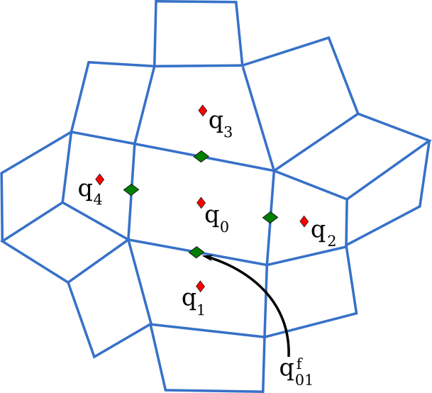
Figure 1: Stencil for reconstruction of fluid variables from cell- to face-centers. USim computes a TVD-style second-order reconstruction of cell-centered data using a combination of the algorithms described in Van Leer (1974) and Mavriplis (2003).

III.2 Riemann Solvers

A version of the Harten-Lax-van Leer approximate Riemann solver Harten et al. (1983) is used in the single-state (HLL, Davis (1988)) and multi-state (HLLD with ‘discontinuities’, Miyoshi and Kusano (2005)) forms. These solvers apply the Rankine-Hugoniot relations that specify the jump in states associated with a subset of the waves of a Riemann problem. For an MHD system, these waves are the fast and slow compressive shocks (two branches each), two branches of an incompressible rotational discontinuity of the magnetic field and velocity associated with the Alfvén wave, and an entropy wave involving only a jump in the density and normal velocity. HLL is a single-state solver that applies jump conditions for the fast discontinuities whereas the HLLD solver is a four-state solver that applies jump conditions for the fast, Alfvén, and contact discontinuities.

The HLL and HLLD approximate Riemann solvers are less diffusive than simpler methods, such as Lax-Friedrichs, while being computationally cheaper than linearized-flux methods that require computation of the full system of eigenvectors (e.g. the methods of Roe Roe (1981) or Serna Serna (2009); Serna and Marquina (2014)). For demonstration purposes we use a Roe method with an arithmetic mean instead of the Roe average as the Roe average is not well-defined for general EOS systems. As demonstrated later, this leads to a ill-posed solution for some non-convex problems. More advanced solvers such as the one proposed by Serna in Ref. Serna and Marquina (2014) overcome this limitation but are not tested in this work.

For the HLL and HLLD approximate Riemann solvers the maximum and minimum signal speeds (eigenvalues) are defined in terms of the reconstructed left and right interface states as in Ref. Davis (1988). Some formulations use a Roe average in this definition Einfeldt et al. (1991), and using a form of the generalized Roe average from Ref. Hu et al. (2009) will be investigated in future work. In isolated cases where the HLLD approximate Riemann solver fails, the simple and robust HLL formulation is used.

III.3 EOS details

For all solvers the fast wave-speeds as modified by a general EOS are used which requires evaluation of the pressure and the generalized sound speed at the interfaces between cells. Two methods are explored for this evaluation: (1) EOS evaluation at the cell centers with reconstruction to the cell interface or (2) direct evaluation of the EOS tables after the MUSCL reconstruction. These methods are more concisely referred to as the cell-centered (CC) and interface (INTF) methods, respectively. The latter method requires more EOS evaluations and is thus more computationally expensive. For example in 3D, where the ratio of cell centers to cell edges is one to eight, we find the total execution time takes 3.5x longer for the INTF method relative to the CC method. For this timing test we use a spline fit to EOS tables with smoothing.

Evaluations of the generalized sound speed, Eqn. (13), requires $P\left(\rho,\varepsilon\right)$ whereas the SESAME EOS tables provide $P\left(\rho,T\right)$ and $\varepsilon\left(\rho,T\right)$. Thus in practice, $\varepsilon\left(\rho,T\right)$ is inverted to find $T\left(\rho,\varepsilon\right)$ which is then used to evaluate $P\left(\rho,T\right)$. The inversion assumes that $\varepsilon\left(\rho,T\right)$ is monotonic in $T$ and $\rho$.

The partial derivatives, $P_{\varepsilon}$ and $P_{\rho}$, are not available within the SESAME tables. Thus evaluation of Eqn. (13) requires some form of numerical differentiation if the tables are not prescribed with an analytic form. The application of the chain rule requires care as the tables typically provide $P\left(\rho,T\right)$ and $\varepsilon\left(\rho,T\right)$ and not $P\left(\rho,\varepsilon\right)$. Thus the partial derivative of pressure with respect to density at constant specific energy is evaluated as

$$P_{\rho}=\left.\frac{\partial P\left(\rho,\varepsilon\right)}{\partial\rho}\right|_{\varepsilon}=\frac{\partial P\left(\rho,T\right)}{\partial\rho}-\frac{\partial P\left(\rho,T\right)}{\partial\varepsilon}\frac{\partial\varepsilon}{\partial\rho}\\ =\frac{\partial P\left(\rho,T\right)}{\partial\rho}-\frac{\partial P\left(\rho,T\right)}{\partial T}\frac{\partial T}{\partial\varepsilon\left(\rho,T\right)}\frac{\partial\varepsilon\left(\rho,T\right)}{\partial\rho}\\ \simeq\frac{\partial P\left(\rho,T\right)}{\partial\rho}-\frac{\partial P\left(\rho,T\right)}{\partial T}\left[\frac{\partial\varepsilon\left(\rho,T\right)}{\partial T}\right]^{-1}\frac{\partial\varepsilon\left(\rho,T\right)}{\partial\rho}\;,$$ (17)

where the last step assumes that $\varepsilon\left(\rho,T\right)$ is monotonic in $T$. Similarly, the partial derivative of pressure with respect to specific energy at constant density is

$$P_{\varepsilon}=\left.\frac{\partial P\left(\rho,\varepsilon\right)}{\partial\varepsilon}\right|_{\rho}=\frac{\partial P\left(\rho,T\right)}{\partial T}\frac{\partial T}{\partial\varepsilon\left(\rho,T\right)}\\ \simeq\frac{\partial P\left(\rho,T\right)}{\partial T}\left[\frac{\partial\varepsilon\left(\rho,T\right)}{\partial T}\right]^{-1}\;,$$ (18)

where again we assume that $\varepsilon\left(\rho,T\right)$ is monotonic in $T$. When analytic derivatives are not available, a finite-difference method is used to evaluate these partial derivatives centered around given values of $\rho$ and $T$ with a stencil size defined in terms of a small $\delta$ (e.g. $10^{-5})$ times $\rho$ and $T$.

Our experience is that a high-order fit to the table data that ensures continuity of the derivative quantities is required to avoid spurious oscillations. Thus for the SESAME results presented in this work, we use a polynomial fit to the data within the region of interest. Another solution is to use spline fits as may be provided through the EOSPAC library Cranfill (1987). We choose the simple polynomial fit as it is sufficiently accurate for our purposes and it is computationally more efficient.

IV 1D test cases

We begin with a series of 1D tests that check the convergence rate of the algorithm with a linearized wave test, Sec. IV.1, and then compare to prior results on Riemann problems, Sec. IV.2.

IV.1 1D linear waves

When a sufficiently small perturbation is placed upon large background fields in a periodic box, it permits analysis through linearization where terms proportional to the square of the perturbation and higher order are dropped. With constant background fields the solution to this system of equations is simply the linear waves. In this test, a small perturbation proportional to the right eigenvector of a given wave of the EOS system is used (see the appendix of Ref. Serna and Marquina (2014) for the right eigenvectors). Perturbing a sinusoidal wave using the right eigenvector associated with a particular characteristic speed results in propagation of the wave at that speed. A computation is run for a single-wave period and the initial and final states are compared. A difference in phase is attributed to dispersive error. Any reduction in wave amplitude is due to diffusive error. By varying the resolution, the calculated L1 error in the eight MHD fields determine the convergence rate.

The vector of conserved variables, given by $\mathbf{Q}$, is perturbed using the right eigenvectors associated with each of the slow-magnetosonic wave $c_{s}$, the fast-magnetosonic wave $c_{f}$, and the Alfvén wave $c_{a}$. The form of the perturbation is $\delta\mathbf{Q}=A\mathbf{R}\sin\left(2\pi\psi\right)$ where $A$ is the perturbation amplitude, $\mathbf{R}$ is the right eigenvector associated with the wave of interest, and $\psi$ is $x/L_{x}$ for 1D, or $x/L_{x}+y/L_{y}$ for 2D (see Sec. V.1).

The SESAME table 5760 SES (1974) is used for helium in this test. The initial conditions for these simulations include a density of $1.0$ $kg/m^{3}$, a pressure of $6.13$ $atm$, and magnetic fields of $\mathbf{B_{0}}=619.4\;\langle 1.0,\sqrt{2.0},0.5\rangle$ $T$. This choice of magnetic fields maintains the same plasma $\beta$ (the ratio of thermal pressure to magnetic pressure) as Stone et al. (2008). The perturbation amplitude is $A=10^{-6}$. We study the convergence of 1D simulations using a refinement factor of $2$ for grid resolutions ranging from $32$ to $1024$ cells for a domain given by $0$ $m\leq x\leq 1$ $m$. The time integration is a third-order Runge-Kutta algorithm.

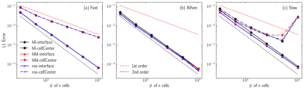
Figure 2: The 1D convergence of the interface- and cell-centered-EOS-evaluation algorithms for the (a) fast magnetosonic, (b) Alfvénic, and (c) slow magnetosonic perturbations, respectively. Separate curves are shown for the HLL, HLLD and Roe approximate Riemann solvers.

Figure 2 compares the L1 error for the linearized wave computations for the three distinct waves, fast, Alfvén, and slow, at varying resolution. The different algorithms for EOS evaluations, as described in Sec. III, are compared. Finally, each algorithm is run with the HLL, HLLD and Roe approximate Riemann solvers which creates six curves per wave. In general, only small variations are evident between the choice of approximate Riemann solver.

Both algorithms achieve the expected second-order convergence with the Alfvén wave (middle plot). This is reasonably expected as this wave is purely magnetic and does not contain a pressure perturbation. However, deficiencies with the cell-centered-EOS evaluations are evident with both the fast and slow waves. For the fast wave, the cell-center-EOS-evaluation algorithm leads to convergence at first order while the interface-EOS-evaluation algorithm performs with the expected second-order convergence. Similarly for slow wave while the interface-EOS-evaluation algorithm performs as expected, dispersion error ultimately leads to the lack of convergence with the cell-centered-EOS-evaluation algorithm. Visually, this dispersion error is barely perceptible although it clearly is evident in the plot of the L1 error.

IV.2 Shock tube

	$\rho_{L}$	$\mathbf{v}_{L}$	$\mathbf{B}_{L}$	$P_{L}$	$\rho_{R}$	$\mathbf{v}_{R}$	$\mathbf{B}_{R}$	$P_{R}$
Dedner01	250	(0,0,0)	(61.752,54.277,0)	35966778.0	179	(-1.7,5.6,0)	(61.752,49.413,0)	26476136.8
DG1	1.8181	(0,0,0)	Tab. 2	3.000	0.275	(0,0,0)	Tab. 2	0.575
DG2	0.879	(0,0,0)	Tab. 2	1.090	0.562	(0,0,0)	Tab. 2	0.885
DG3	0.879	(0,0,0)	Tab. 2	1.090	0.275	(0,0,0)	Tab. 2	0.575

Table 1: Initial conditions for the shock tube tests from Refs. Dedner and Wesenberg (2001) and Serna and Marquina (2014). Units are in $kg/m^{3}$, $m/s$, $mT$ and $Pa$, respectively, but are not particularly meaningful for this problem.

	$\mathbf{B}_{L}$	$\mathbf{B}_{R}$
MHD-DG1-O	(38.114,38.114,0)	same
MHD-DG1-T	(0,50.445,0)	same
MHD-DG2-O	(34.751,34.751,0)	same
MHD-DG2-T	(0,48.203,0)	same
MHD-DG3-O	(44.840,67.260,0)	same
MHD-DG3-T	(0,42.598,0)	same
MHD-DG3-R-O	(44.840,67.260,0)	(44.840,-67.260,0)
MHD-DG3-L-O	(112.10,112.10,0)	same

Table 2: Initial magnetic conditions for the shock tube tests from Ref. Serna and Marquina (2014). Units are in $mT$.

	$R$	$C_{V}$	$\eta_{a}$	$\eta_{b}$
Dedner (Ref. Dedner and Wesenberg (2001))	461.5	1401.88	1684.54	0.001692
Serna (Ref. Serna and Marquina (2014))	1	80	3	$1/3$

Table 3: Van Der Waals model parameters for to characterize the EOS of Eqn. (7) for the shock tube tests from Ref. Serna and Marquina (2014).

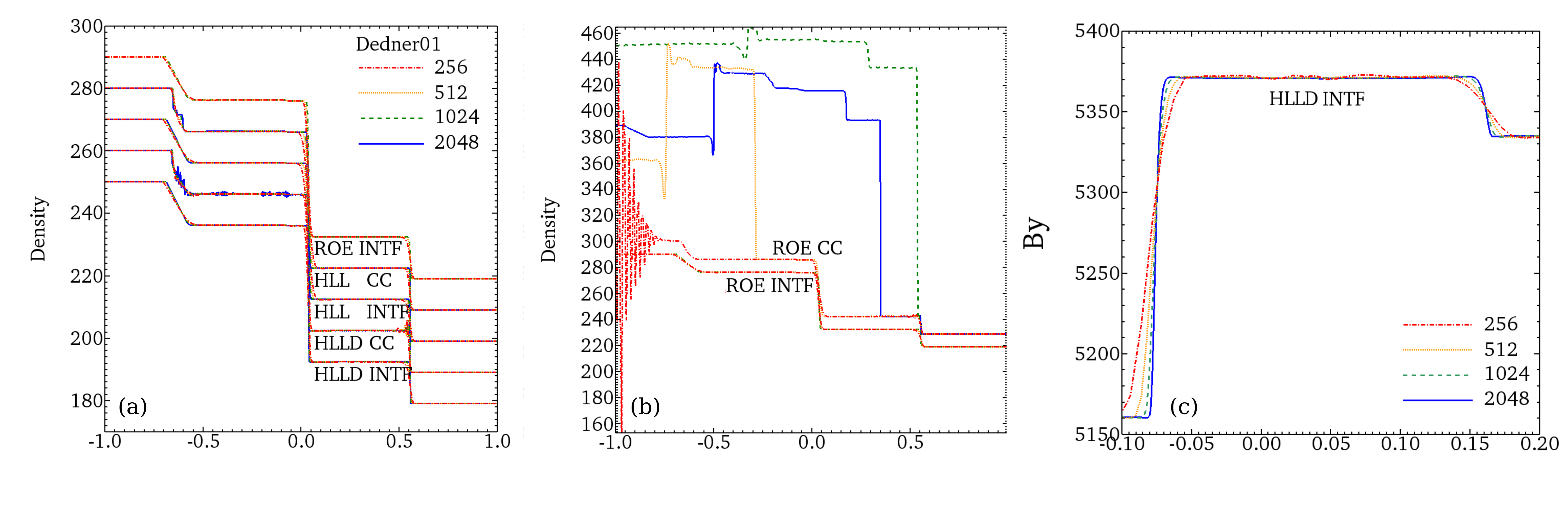
Figure 3: Six different algorithms compared to the results of the shocktube test from Ref. Dedner and Wesenberg (2001), Fig. 6. In figures (a) and (b) the density from a subset of five of the six algorithms and two of the six algorithms are shown, respectively. The curves are grouped by resolution and are offset by multiples of 10 $kg/m^{3}$ to allow for comparison. The six different algorithms are the combinations of the Roe with an arithmetic average, HLL and HLLD approximate Riemann solvers and cell-centered- and interface-EOS-evaluation algorithms. In figure (c) the y-component of the magnetic field is plotted for the HLLD solver with the interface-EOS-evaluation algorithm at different varied resolution.

In this section we compare computations with the known results of shock-tube test cases from Refs. Dedner and Wesenberg (2001) and Serna and Marquina (2014). The initial conditions for these cases are given in Tabs. 1 and 2. These cases use the Van Der Waals EOS with the parameters as listed in Tab. 3. The time integration is a second-order Runge-Kutta algorithm.

In Fig. 3 different methods are compared to the MHD shocktube case shown in Fig. 6 of Ref. Dedner and Wesenberg (2001). Six different algorithms are compared: the combinations of the Roe with an arithmetic average, HLL and HLLD approximate Riemann solvers and cell-centered- and interface-EOS evaluation algorithms. In the Fig. 3(a), the density at t=0.001 is plotted for all of these algorithms except Roe with cell-centered-EOS evaluation. The results are grouped by spatial resolution and offset by constant factors from the HLLD with interface EOS evaluation result to enable quick comparison. The expected result from left to right is a compression fan associated with the leftward propagating fast magnetosonic wave, a shock associated with the leftward propagating slow magnetosonic wave (the jump in the density is very small), a contact discontinuity, a shock associated with the rightward propagating slow magnetosonic wave (the jump in the density is again very small), and a shock associated with the rightward propagating fast magnetosonic wave. The interface-EOS-evaluation algorithm agrees well with the expected results regardless of the choice of the approximate Riemann solver. However, while the cell-centered-EOS-evaluation produces a somewhat reasonable result at low resolution (except for an incorrect jump appearing in the leftward compression fan that then appears as a compound wave), substantial noise appears as the resolution is increased. The appearance of this noise is associated with the magnetosonic waves consistent with the dispersion error observed in the 1D linear wave tests in Sec. IV.1. In Fig. 3(b) the result for the Roe solver with an arithmetic average with cell-centered EOS evaluation is also shown. This algorithm produces a clearly incorrect result, particularly at high resolution. In Fig. 3(c) the y-component of the magnetic field is plotted for the HLLD solver with the interface EOS evaluation algorithm at different varied resolution. The convergence of this algorithm is favorable compared to the algorithms tested in Ref. Dedner and Wesenberg (2001) as seen by comparing to Fig. 6(b) of that work.

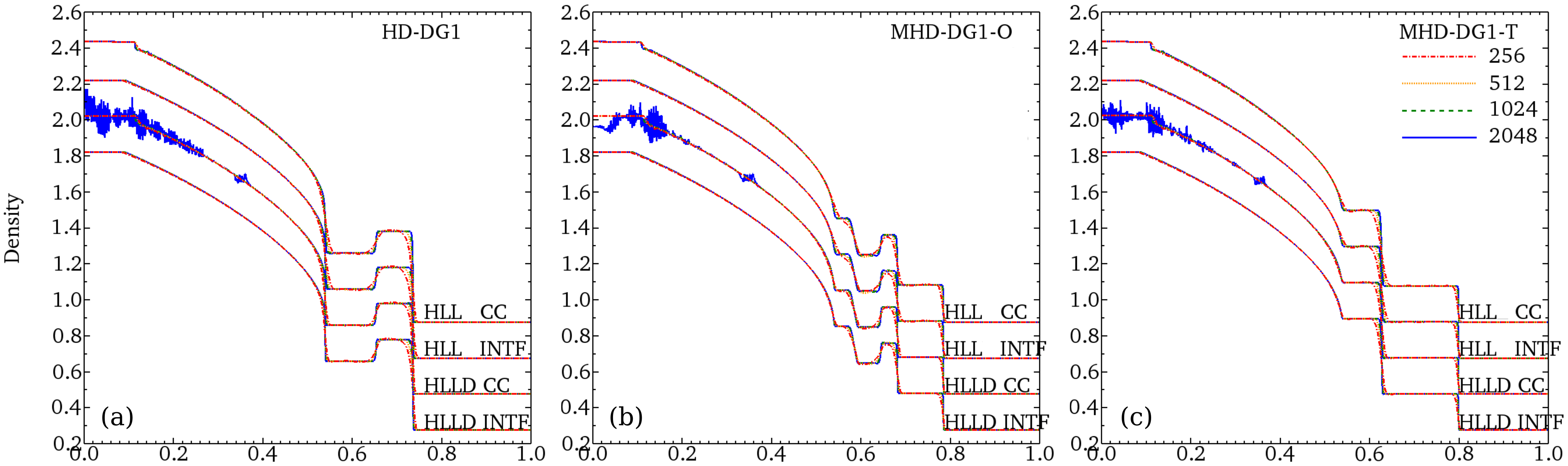
Figure 4: Four different algorithms compared to the results of the DG1 shocktube test at t=0.15 from Ref. Serna and Marquina (2014), Fig. 1. The four different algorithms are the combinations of the HLL and HLLD approximate Riemann solvers and cell-centered- and interface-EOS-evaluation algorithms. The density from the (a) hydrodynamic, (b) oblique-magnetic-field, and (c) transverse-magnetic-field versions of the tests are shown. The curves are grouped by resolution and are offset by multiples of 0.2 $kg/m^{3}$ to allow for comparison.

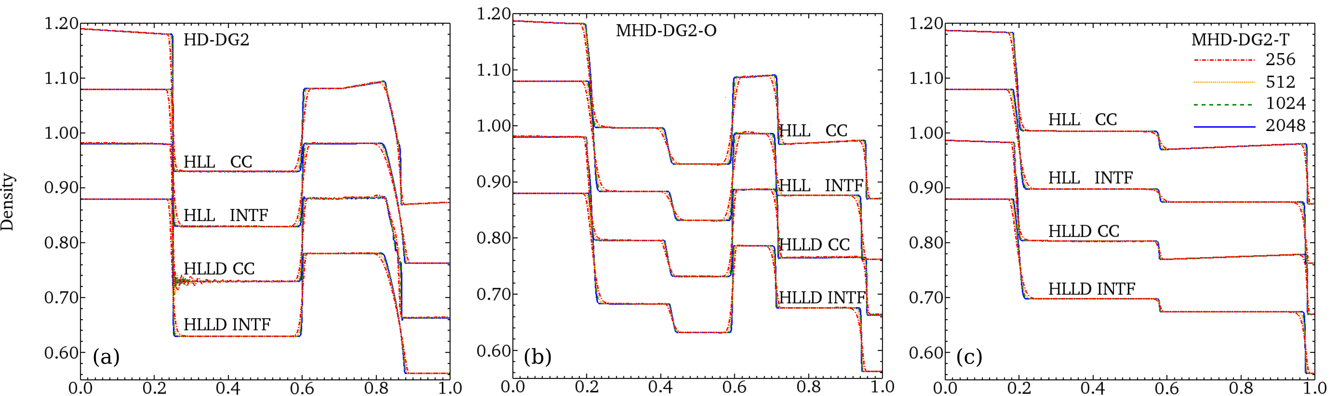
Figure 5: Four different algorithms compared to the results of the DG2 shocktube test at t=0.45 from Ref. Serna and Marquina (2014), Fig. 2. The four different algorithms are the combinations of the HLL and HLLD approximate Riemann solvers and cell-centered- and interface-EOS-evaluation algorithms. The density from the (a) hydrodynamic, (b) oblique-magnetic-field, and (c) transverse-magnetic-field versions of the tests are shown. The curves are grouped by resolution and are offset by multiples of 0.1 $kg/m^{3}$ to allow for comparison.

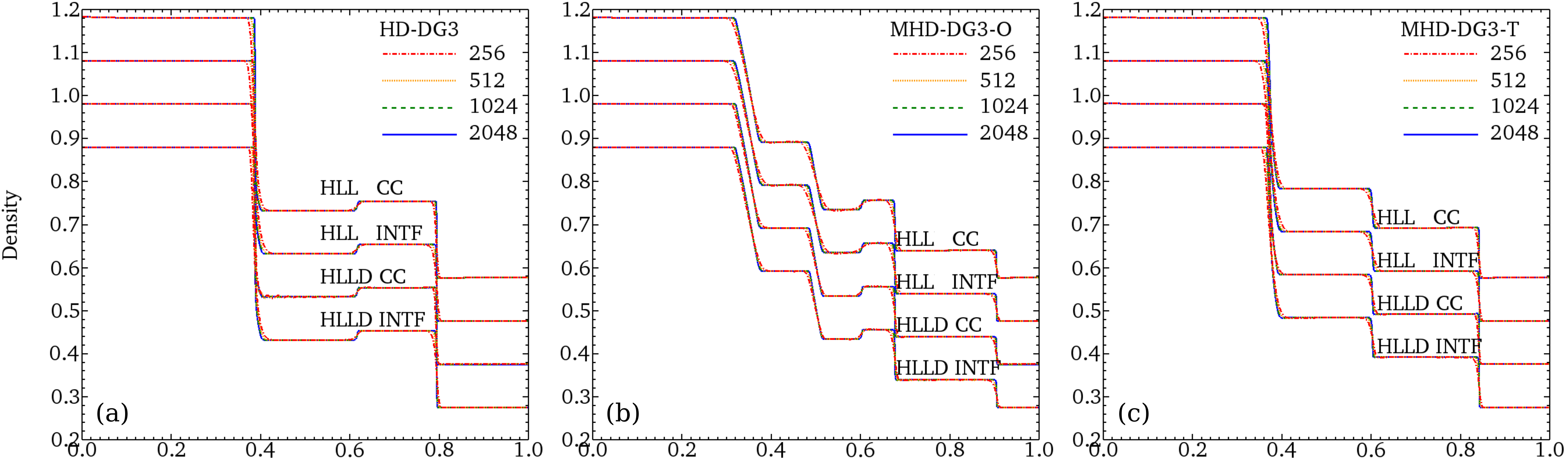
Figure 6: Four different algorithms compared to the results of the DG3 shocktube test at t=0.2 from Ref. Serna and Marquina (2014), Fig. 3. The four different algorithms are the combinations of the HLL and HLLD approximate Riemann solvers and cell-centered- and interface-EOS-evaluation algorithms. The density from the (a) hydrodynamic, (b) oblique-magnetic-field, and (c) transverse-magnetic-field versions of the tests are shown. The curves are grouped by resolution and are offset by multiples of 0.1 $kg/m^{3}$ to allow for comparison.

Next we compare results from the shocktube tests of Ref. Serna and Marquina (2014) in Figs. 4-6. These should be compared to Figs. 3-5 of Ref. Serna and Marquina (2014). Each of these tests start with a pure hydrodynamic case (HD) without magnetic field. Evaluation of the thermodynamic fundamental derivative shows that all of these cases produce non-convex dynamics with anomalous waves for the hydrodynamic cases Serna and Marquina (2014). As such, the ability of the scheme to produce solutions comparable with those of Ref. Serna and Marquina (2014) is a useful indicator of its ability to address non-convex EOS in a robust fashion; such a capability is critical for algorithms that address real materials, due to the presence of non-convex behavior within tabular EOS. Furthermore, the presence of oblique (MHD-O) and transverse (MHD-T) magnetic field within the test modifies the overall convexity of the system. In the cases presented here, the presence of these magnetic fields act to increase the convexity of the overall system; accurately capturing this interplay is important to understanding the interaction of magnetic fields with real materials.

In Figs. 4, 5 and 6 the results of the DG1-DG3 cases are shown. For all of these cases, the Roe solver with an arithmetic average fails to produce a numerical solution and we do not include it in this discussion. From left to right for the HD case, there is a expansion shock or rarefaction fan, an entropy wave and compression shock or fan. For the DG1 and DG2 cases, Figs. 4 and 5 respectively, the cell-centered-EOS-evaluation algorithm produces an errant feature at the top of the leftmost expansion and with the relatively low dissipation HLLD solver spurious oscillations are observed at high resolution. All algorithms perform well on the DG3 case in Fig. 6 (this is also true for the rotated-oblique-magnetic-field and large-oblique-magnetic-field versions of DG3 from Ref. Serna and Marquina (2014) which are not shown). With the addition of oblique (MHD-O) and transverse (MHD-T) magnetic field additional waves are produced as associated with the MHD system. The result of comparison of the cell-centered- and interface-EOS-evaluation algorithms is comparable to that found with the HD results.

V 2D test cases

Next we apply our algorithm to 2D systems to check the performance with multiple dimensions. The tests progress in order of increasing complexity: first a linear wave test of convergence, Sec. V.1, then the nonlinear circularly-polarized Alfven wave test, Sec. V.2, which checks both convergence for a problem with a large amplitude perturbation but also tests the accuracy of the algorithm. Finally, we conclude with a test using the magnetized Rayleigh-Taylor instability, Sec. V.3, which fully demonstrates the limitations of the cell-centered reconstruction algorithm.

V.1 2D linearized waves

The two-dimensional linearized-waves tests are an extension of the 1D tests from Sec. IV.1. In 2D, the vector components of $\mathbf{Q}$ undergo a rotational transformation to create a propagation oblique to the grid. The 2D simulations use a structured, Cartesian domain ($0$ $m\leq x\leq 2$ $m$ and $0$ $m\leq y\leq 1$ $m$) with twice the grid resolution in the x-direction compared to the y-direction. Since the grid is rectangular, and the cells are square, the transformed perturbation along the rectangular diagonal ensures that the x and y fluxes differ in magnitude for each cell; thereby ensuring the simulation is truly 2D. The convergence tests start with a grid resolution in the y-direction of $8$ cells and is ultimately enhanced to $256$.

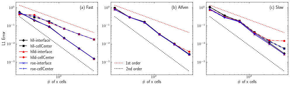
Figure 7: The 2D convergence of the interface- and cell-centered-EOS-evaluation algorithms for the (a) fast magnetosonic, (b) Alfvénic, and (c) slow magnetosonic perturbations, respectively. Sepearate curves are shown for the HLL, HLLD and Roe approximate Riemann solvers.

Figure 7 shows the convergence of the interface- and cell-centered- EOS-evaluation algorithms for the (a) fast-magnetosonic, (b) Alfvénic, and (c) slow-magnetosonic perturbations, respectively. Separate curves are shown for the HLL, HLLD and Roe approximate Riemann solvers. The convergence in 2D is comparable to the 1D result from Fig. 2. For the interface-EOS-evaluation algorithm, the expected second-order convergence for all waves is produced. However, the results for the cell-centered-EOS-evaluation algorithm are mixed: Although the Alfvén wave converges with second-order accuracy, the fast-magnetosonic wave converges only at first order. The slow-magnetosonic wave initially converges with second-order accuracy but it ultimately produces large errors at high resolution resulting from dispersion. Again this result shows the importance of consistent EOS evaluation for the compressive magnetosonic waves.

V.2 Nonlinear 2D circularly polarized Alfvén wave

Next we examine a nonlinear circularly-polarized Alfvén wave test which checks both convergence for a problem with a large amplitude perturbation but also tests the accuracy of the algorithm. This test is based off a version from Ref. Tóth (2000) but is modified to the grid and wave orientation from Ref. Gardiner and Stone (2005). In this form, the initial state is $\rho=1$, $p=\beta b^{2}/2$,

$$\begin{split}\rho u_{x}&=-0.1sin(\alpha)sin(2\pi x_{\parallel})\;kg\,m^{-2}\,s^{-1}\\ \rho u_{y}&=0.1cos(\alpha)sin(2\pi x_{\parallel})\;kg\,m^{-2}\,s^{-1}\\ \rho u_{z}&=0.1cos(2\pi x_{\parallel})\;kg\,m^{-2}\,s^{-1}\\ B_{x}&=cos(\alpha)-0.1sin(\alpha)sin(2\pi x_{\parallel})\;\sqrt{\mu_{0}}\,T\\ B_{y}&=sin(\alpha)+0.1cos(\alpha)sin(2\pi x_{\parallel})\;\sqrt{\mu_{0}}\,T\\ B_{z}&=0.1cos(2\pi x_{\parallel})\;\sqrt{\mu_{0}}\,T.\end{split}$$ (19)

where the parallel direction to the wavevector is given by $x_{\parallel}=xcos(\alpha)+ysin(\alpha)$. This leads to a constant magnetic-field energy of $0.505$ $J/m^{3}$. The domain is zero to $1/cos(\alpha)$ in the x direction and zero to $1/sin(\alpha)$ in the y direction with $\alpha=\pi/2-atan(0.5)\simeq 63.4^{\circ}$. The number of x cells is twice the y cells such that each cell is then square and propagation is oblique to the grid. The time integration is a third-order Runge-Kutta algorithm. The Van Der Waals (Eqn. (7)) model parameters for the non-ideal EOS computations are $R=2.077$, $C_{V}=3.116$, $\eta_{a}=9.213\times 10^{-4}$ and $\eta_{b}=9.513\times 10^{-2}$. These parameters are chosen such that there is an approximately 10% variation to the EOS relative to the ideal-gas EOS.

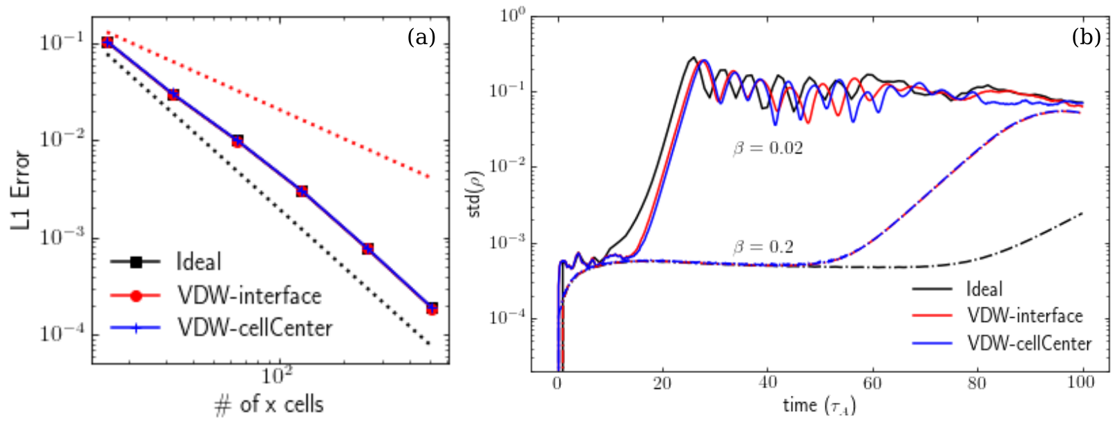
Figure 8: Results from the circularly polarized Alfvén wave test. Subfigure (a) shows the L1 error in the momentum after a single period of oscillation of the wave for the ideal model and the Van Der Waal model with the cell-centered- and interface-EOS-evaluation algorithms. Subfigure (b) shows the standard deviation of the density with respect to time for the three algorithms/models at two different values of $\beta$.

Figure 8(a) plots the L1 error in the momentum after a single period of oscillation of the wave for the ideal model and the Van Der Waal model with the cell-centered- and interface-EOS-evaluation algorithms. Convergence of the algorithm is second order for all cases consistent with the discussions of Secs. IV.1 and V.1.

As described in Ref. Del Zanna, L. et al. (2001) it is known that the circularly-polarized Alfvén wave is subject to a parametric instability that causes it to decay into a magnetosonic wave. The rate of decay is inversely proportional to the plasma $\beta=2\mu_{0}p/B^{2}$. Similar to Ref. Del Zanna, L. et al. (2001) we examine the time dynamics of this parametric decay in simulations at two values of $\beta$ and varied numerical algorithms and/or models: the HLLD approximate Riemann solver with an ideal-gas EOS and a Van Der Waals EOS with either interface- or cell-centered-EOS evaluations. Unlike Ref. Del Zanna, L. et al. (2001), we do not seed our simulation with random noise, thus we expect the parametric instability to rise purely from numerical error.

Fig. 8(b) shows the standard deviation of the density with respect to time for the three algorithms/models at two different values of $\beta$ for a fixed grid resolution of 128$\times$64. A large standard deviation of the density indicates that compressional magnetosonic dynamics have become large with the simulation entering a turbulent state. As the growth rate is inversely proportional to $\beta$, at $\beta=0.02$ the instability grows faster than at $\beta=0.2$. For both cases the sound speed is approximately 5% greater for the Van Der Waals EOS ($c_{s}=0.136$ m/s) relative to the ideal gas EOS ($c_{s}=0.13$ m/s). For both values of $\beta$, the cell-centered EOS evaluation algorithm performs nearly identical to the interface EOS evaluation algorithm until well after a saturated state is achieved. As the instability is seeded by numerical error, this reinforces the results of Sec. IV.1 and V.1 in that the error associated with the Alfvén wave is comparable between these algorithms.

V.3 Magneto-Rayleigh-Taylor instability

Finally, we examine the performance of the EOS algorithms with the classical single-mode Magnetic Rayleigh-Taylor (MRT) instability simulation from Ref. Stone et al. (2008). Our computations differ from the prior work as more realistic densities, pressures, and temperatures for the ideal gas helium are used with the SESAME-5760 EOS similar to Secs. IV.1 and V.1. In this test, a heavy plasma is supported by a light plasma at constant pressure in the presence of a gravitational acceleration and a transverse magnetic field. This configuration is an inherently unstable equilibrium, and the vertical velocity in the direction of the acceleration is sinusoidally perturbed to seed the instability.

Initial conditions for this simulation are $\rho_{h}=5.0$ kg/m³, $\rho_{l}=0.5\rho_{h}$, $P_{0}=2$ atm, $g=24.0$ km/s², and $\vec{B}=\langle 25.0,\,0.0,\,0.0\rangle\;mT$ which correspond to heavy-fluid density, light-fluid density, atmospheric pressure, gravitational acceleration, and the magnetic field, respectively. The constant $g$ is chosen such that the buoyancy pressure ($=\rho gy$) is $P_{b}\approx 0.06P_{0}$ ensuring the MRT interface, the boundary between the heavy and light fluid, remains relatively fixed, and coincidentally the gage pressure $P=P_{0}-P_{b}=P_{0}-\rho gy$ does not go negative while still allowing for a reasonable growth rate given the spatial scales. The magnetic field is chosen so that the simulation is spatially converged late in time, and not overly stabilized. Without a magnetic field the numerical error from the development of mesh-scale features outweighs any different dynamics introduced from using a real-gas EOS which makes comparison difficult.

The domain is $L_{x}=1$ $m$, and the range is $L_{y}=2$ $m$, with a grid resolution of 200$\times$400 where the origin is chosen such that $x\epsilon[-L_{x}/2,L_{x}/2]$, and $y\epsilon[-L_{y}/2,L_{y}/2]$. Boundary conditions for the y-direction are non penetrating, and for the x-direction are periodic. The time integration is a second-order Runge-Kutta algorithm.

The widely known classical linear growth rate of the MRT instability is given by

$$\gamma=\sqrt{kgA-\frac{(\vec{k}\cdot\vec{B})^{2}}{\mu_{0}(\rho_{h}+\rho_{l})}}$$ (20)

where $\vec{k}$ is the perturbation wavevector which has magnitude $k=2\pi$ $m^{-1}$ and $A$ is known as the Atwood number which is $A=(\rho_{h}-\rho_{l})/(\rho_{h}+\rho_{l})=1/3$. For the test conditions $\gamma\approx 218$ $s^{-1}$ which is used to calculate an simulation time of $6.0/\gamma\approx 27.5$ $ms$. This time allows for sufficient mode growth well into the nonlinear regime. The derivation of the linear growth rate does not assume an ideal-gas EOS, and this allows direct comparison of MRT growth between the different EOS algorithms. The functional form of the perturbation on the vertical velocity is a single sinusoid with $\lambda$ equivalent to the domain size $L_{x}$, and is given by

$$\delta v=-\delta\left(1+\cos(kx)\right)\exp\left[\frac{-20y^{2}}{L_{y}^{2}}\right]\;,$$ (21)

where $\delta$ is the perturbation amplitude which is $6.6$ $m/s$.

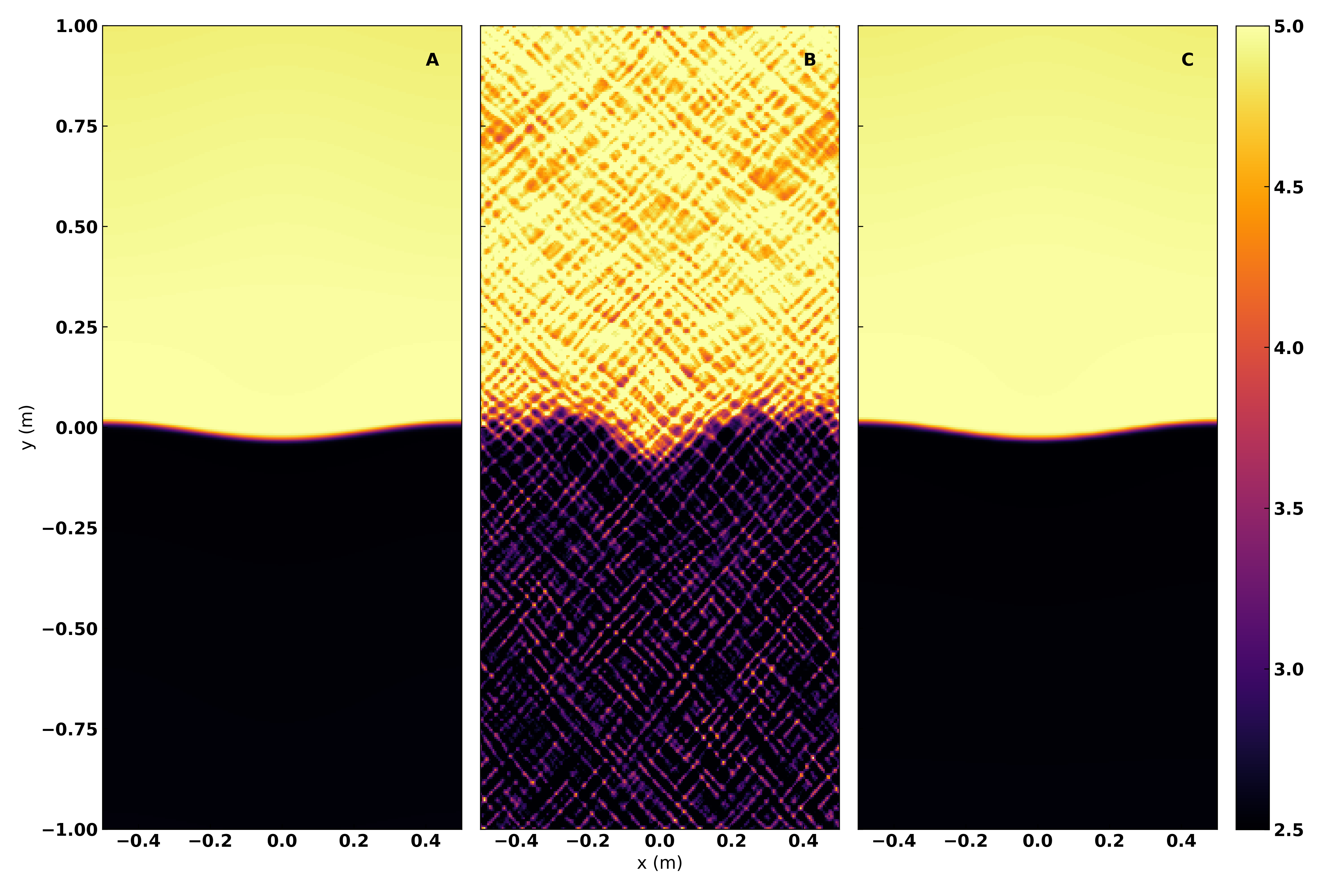
Figure 9: The early-time density state in kg/m³ ($t=3.3\;ms$) of the 2D MRT instability growth of density in kg/m³ for the (A) ideal-gas EOS, (B) the SESAME-5760 EOS using the cell-centered EOS evaluation algorithm, and (C) the SESAME 5760-EOS using the interface EOS evaluation algorithm.

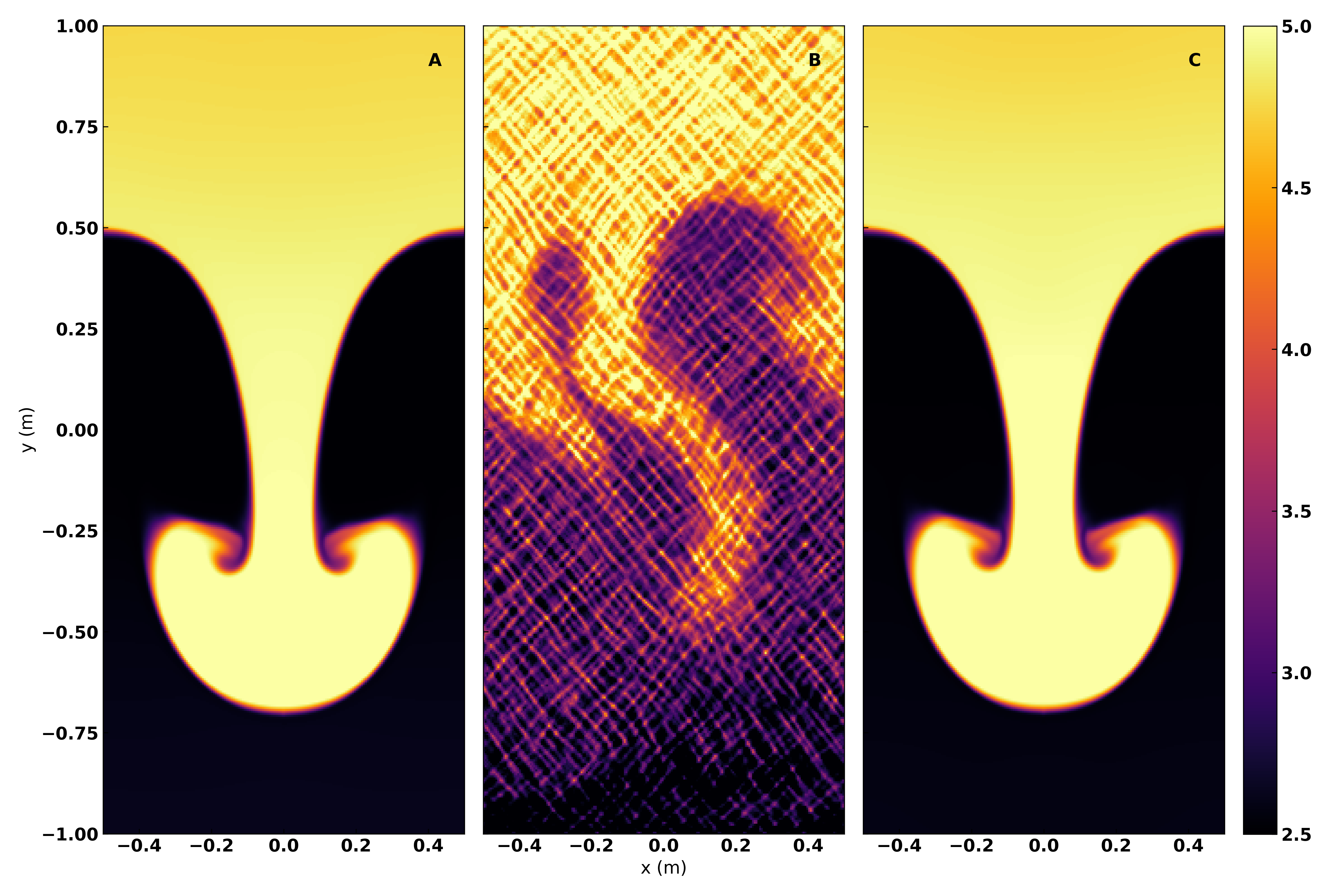
Figure 10: The final density state in kg/m³ ($t=27.5\;ms$) of the 2D MRT instability growth of density in kg/m³ for the (A) ideal-gas EOS, (B) the SESAME-5760 EOS using the cell-centered EOS evaluation algorithm, and (C) the SESAME 5760-EOS using the interface EOS evaluation algorithm.

Figures 9 and 10 show the growth of the MRT instability early and late in time, respectively. Examination of these figures highlights the differences between the different EOS-evaluation algorithms. Consistent with the results of Secs. IV.1, IV.2 and V.1 which demonstrated potential issues with the cell-centered-EOS-evaluation algorithm, poor results are observed with the cell-centered-EOS-evaluation algorithm (B) relative to computations with an ideal-gas EOS (A) and the interface-EOS-evaluation algorithm (C). However, unlike the prior results which produced somewhat qualitatively consistent results with the cell-centered-EOS-evaluation algorithm, the MRT test shows that computations with this algorithm can be completely unreliable. As seen in Fig. 9(B), the cell-centered-EOS-evaluation algorithm generates spurious sound waves almost immediately. By the end of the simulation, Fig. 10(B), this leads to unphysical results. The results of the ideal gas model (A) are qualitatively identical to the use of the interface-EOS-evaluation algorithm (C) with only small differences in magnitude at the simulation end while the propagation distance and mode number are the same. As the linear-MRT analysis is not dependent on the EOS, this indicates that the interface-EOS-evaluation algorithm is convincingly more accurate than the cell-centered-EOS-evaluation algorithm.

VI Discussion and Summary

This work evaluates algorithms that model applications described by magnetohydrodynamics with a real-gas Equation-of-State in multiple dimensions. The approximate Riemann solvers employed take the HLL form and two methods of evaluation of the Equation-of-State are proposed: at the cell centers or directly at the interfaces between cells. Although the former method is computationally more efficient that the latter, we demonstrate that such an approach lacks robustness through a suite of one- and two-dimensional tests. For example, the cell-centered-EOS-evaluation algorithm exhibits poor convergence with the linear magnetosonic waves in both 1D and 2D. In addition to this failure, the cell-centered-EOS-evaluation algorithm produces spurious results for 1D shock tube test problems at high resolution using an HLLD-type Riemann solver. We note that the shock tube test problems considered here probe EOS that include non-convex behavior, indicated through the fundamental thermodynamic derivative passing from positive to negative Serna and Marquina (2014). These tests therefore demonstrate the ability of the scheme to capture behavior that is expected to occur in tabular EOS associated with real materials. By contrast, the interface-EOS-evaluation algorithm produces high quality results for this problem set at high resolution with the HLLD Riemann solver. Overall, results for these shock tubes indicate that the interface-EOS-evaluation algorithm may be more robust for tabular EOS associated with real materials, even when combined with Riemann-solvers that minimize numerical dissipation.

That the cell-centered-EOS-evaluation algorithm lacks robustness for real EOS is demonstrated by a 2D magneto-Rayleigh-Taylor instability test problem, where this algorithm completely fails to produce reasonable results. These are characterized by a checker board pattern that exhibits in the density at early times during the linear growth phase of the instability and completely corrupts the development of the characteristic MRT fingers that characterize the instability. By contrast, the interface-EOS-evaluation algorithm is able to accurately capture the linear growth of this 2D magneto-Rayleigh-Taylor instability, demonstrating the growth of the characteristic MRT fingers in a fashion at least qualitatively comparable to the development of the instability in an ideal gas. Since the linear growth phase of the instability is independent of the EOS, the qualitative similarity of the results produced by the scheme for both ideal and real gas (tabular) EOS serves to enhance confidence in the interface-EOS-evaluation algorithm, while demonstrating the unsuitability of the cell-centered-EOS-evaluation scheme.

This work is a first step on the route to developing robust, peer-reviewed algorithms for combining magnetohydrodynamics with EOS for real materials. Our principle conclusion is that the EOS must be evaluated collocated with points for computation of numerical fluxes in order to produce a robust algorithm, capable of accurately capturing MHD effects in real materials. As such, our conclusions have important implications for the design of schemes that combine higher order finite volume and/or discontinuous Galerkin methods for MHD with real EOS. However, in demonstrating this conclusion, we have considered a single material; however, real experiments often consist of multiple materials, each with an equation of state that may exhibit different behavior. A range of methodologies for mixing together EOS for different materials exist Magyar et al. (2014), which amount, in general to different rules for mixing together material pressures in either either a linear or non-linear fashion dependent on the fractional densities. We note that Ref. Magyar et al. (2014) found that a mixing model based on the (non-linear) Amagat’s rule works reliably in the multi Mbar and several thousand degree temperature range that characterizes high energy density environments. In principle, such a rule can be combined with algorithms that track species mass fractions (such as those considered by, e.g. Ref. Hu et al. (2009)) in order to develop an algorithm that enables mixed materials with real EOS, which can, in turn, be combined with the MHD algorithms developed here. Care, however, is needed, to ensure that such an algorithm appropriately captures the convexity of the system when combined with magnetic fields, as discussed by Ref. Serna and Marquina (2014) and shown to be the case for the algorithms here in Sec. IV.2. Furthermore, high energy density systems often exist in strong coupling regimes, where the ionic Coulomb interaction dominates over the ion thermal energy Stanton and Murillo (2015). In such systems, it is challenging to separate the EOS from the Coulomb interaction and develop fluid models that sit on a rigorous theoretical foundation Diaw and Murillo (2019); Baalrud and Daligault (2019); the case including magnetic fields, which, in the fluid limit, would yield MHD models that consistently incorporate real materials EOS and strong coupling appropriate for high energy density plasmas is, as yet, an unsolved problem. We leave detailed consideration of all of these issues to future work.

References

- LeVeque (2002) R. J. LeVeque, Finite-Volume Methods for Hyperbolic Problems (Cambridge University Press, 2002).
- Einfeldt (1988) B. Einfeldt, SIAM Journal on Numerical Analysis 25, 294 (1988).
- Roe (1981) P. Roe, Journal of Computational Physics 43, 357 (1981).
- Buffard et al. (2000) T. Buffard, T. Gallouët, and J.-M. Hérard, Computers and Fluids 29, 813 (2000).
- Coquel and Perthame (1998) F. Coquel and B. Perthame, SIAM Journal Numerical Analysis 35, 2223 (1998).
- Hu et al. (2009) X. Hu, N. Adams, and G. Iaccarino, Journal of Computational Physics 228, 6572 (2009).
- Harten et al. (1983) A. Harten, P. Lax, and B. Leer, SIAM Review 25, 35 (1983), https://doi.org/10.1137/1025002 .
- Toro et al. (1994) E. F. Toro, M. Spruce, and W. Speares, Shock Waves 4, 25 (1994).
- Dedner and Wesenberg (2001) A. Dedner and M. Wesenberg, “Numerical methods for the real gas mhd equations,” in Hyperbolic Problems: Theory, Numerics, Applications: Eighth International Conference in Magdeburg, February/March 2000 Volume 1 (Birkhäuser Basel, 2001) pp. 287–296.
- Serna and Marquina (2014) S. Serna and A. Marquina, Physics of Fluids 26, 016101 (2014).
- Serna (2009) S. Serna, Journal of Computational Physics 228, 4232 (2009).
- Davis (1988) S. Davis, SIAM Journal on Scientific and Statistical Computing 9, 445 (1988), https://doi.org/10.1137/0909030 .
- Miyoshi and Kusano (2005) T. Miyoshi and K. Kusano, Journal of Computational Physics 208, 315 (2005).
- Lyon and Johnson (1992) S. P. Lyon and J. D. Johnson, SESAME: The Los Alamos National Laboratory Equation Of State Database, Tech. Rep. LA-UR-92-3407 (Los Alamos National Laboratory, 1992).
- Macfarlane et al. (2006) J. J. Macfarlane, I. E. Golovkin, and P. R. Woodruff, Journal of Quantitative Spectroscopy and Radiative Transfer 99, 381 (2006).
- Loverich et al. (2013) J. Loverich, S. C. D. Zhou, K. Beckwith, M. Kundrapu, M. Loh, S. Mahalingam, P. Stoltz, and A. Hakim, in 51st AIAA Aerospace Sciences Meeting including the New Horizons Forum and Aerospace Exposition (Grapevine, Texas, 2013).
- Van Leer (1974) B. Van Leer, Journal of computational physics 14, 361 (1974).
- Stone and Gardiner (2009) J. M. Stone and T. Gardiner, New Astronomy 14, 139 (2009).
- Tóth (2000) G. Tóth, Journal of Computational Physics 161, 605 (2000).
- Mignone and Tzeferacos (2010) A. Mignone and P. Tzeferacos, Journal of Computational Physics 229, 2117 (2010).
- Dedner et al. (2002) A. Dedner, F. Kemm, D. Kröner, C.-D. Munz, T. Schnitzer, and M. Wesenberg, Journal of Computational Physics 175, 645 (2002).
- Mavriplis (2003) D. Mavriplis, “Revisiting the least-squares procedure for gradient reconstruction on unstructured meshes,” in 16th AIAA Computational Fluid Dynamics Conference (American Institute of Aeronautics and Astronautics, 2003).
- Einfeldt et al. (1991) B. Einfeldt, C. Munz, P. Roe, and B. Sjögreen, Journal of Computational Physics 92, 273 (1991).
- Cranfill (1987) C. W. Cranfill, The EOSPAC utility package for accessing the Sesame data library, Tech. Rep. X7-87-U53 (Los Aamos National Laboratory, 1987).
- SES (1974) he-4, Tech. Rep. UCIR-740 (Lawrence Livermore Laboratory, 1974).
- Stone et al. (2008) J. M. Stone, T. A. Gardiner, P. Teuben, J. F. Hawley, and J. B. Simon, The Astrophysical Journal Supplement Series 178, 137 (2008).
- Gardiner and Stone (2005) T. A. Gardiner and J. M. Stone, Journal of Computational Physics 205, 509 (2005).
- Del Zanna, L. et al. (2001) Del Zanna, L., Velli, M., and Londrillo, P., A&A 367, 705 (2001).
- Magyar et al. (2014) R. J. Magyar, S. Root, and T. R. Mattsson, Journal of Physics: Conference Series 500, 162004 (2014).
- Stanton and Murillo (2015) L. G. Stanton and M. S. Murillo, Phys. Rev. E 91, 033104 (2015).
- Diaw and Murillo (2019) A. Diaw and M. S. Murillo, Phys. Rev. E 99, 063207 (2019).
- Baalrud and Daligault (2019) S. D. Baalrud and J. Daligault, Physics of Plasmas 26, 082106 (2019), https://doi.org/10.1063/1.5095655 .