Bottlenecks for Weil-Petersson geodesics

Abstract.

We introduce a method for constructing Weil-Petersson (WP) geodesics with certain behavior in the Teichmüller space. This allows us to study the itinerary of geodesics among the strata of the WP completion and its relation to subsurface projection coefficients of their end invariants. As an application we demonstrate the disparity between short curves in the universal curve over a WP geodesic and those of the associated hyperbolic $3$–manifold.

1. Introduction

In this paper we explore some questions about visibility in the Weil-Petersson geodesic flow in Teichmüller space, and its connections to synthetic aspects of the flow, by which we mean the combinatorial behavior of geodesic flow lines for large times. Our motivation is partly the analogy between Weil-Petersson flow and Teichmüller flow, and partly the connections between Weil-Petersson geometry and the geometry of hyperbolic $3$–manifolds.

Our main result is a criterion (Theorem 1.2) for existence of bottlenecks between certain (non-recurrent) pairs of geodesics, and its consequences for visibility, that is to say connectivity by geodesics of certain points at infinity. We use this result to construct examples of geodesics whose approach pattern to the completion strata of the Teichmüller space exhibits some new phenomena (Theorems 1.3, and 5.5), and related examples in which the connection between WP geometry and hyperbolic geometry breaks down (Theorems 1.4 and 1.5).

Bottlenecks and visibility

A bottleneck for a pair $R,R^{\prime}$ of subsets of a geodesic metric space $\operatorname{\mathcal{X}}$ is a compact set $K\subsetneq\operatorname{\mathcal{X}}$ such that every geodesic segment with endpoints on $R$ and $R^{\prime}$ meets $K$.

For two geodesic rays $r,r^{\prime}$, visibility of their endpoints at infinity is the existence of a geodesic $g$ strongly asymptotic to $r$ in forward time and $r^{\prime}$ in backward time. The existence of a bottleneck is an important step in the proof of visibility.

For example, it is shown in [BMM10, Theorem 1.3] that any two recurrent geodesic rays have a bottleneck and satisfy the corresponding visibility property. To consider the non-recurrent case we start with geodesics that are asymptotic to completion strata in Teichmüller space. If $\omega$ is a multicurve in $S$, let $\ell_{\omega}:\operatorname{Teich}(S)\to\operatorname{\mathbb{R}}_{+}$ be its geodesic length function on Teichmüller space. The stratum $\operatorname{\mathcal{S}}(\omega)$ is the locus in the Weil-Petersson completion of $\operatorname{Teich}(S)$ where the curves of $\omega$ are replaced by punctures (hence $\ell_{\omega}=0$). The following conjecture seems reasonable but is currently beyond our reach:

Conjecture 1.1.

Let $\omega,\omega^{\prime}$ be two multicurves in $S$ that fill the surface. Then $\operatorname{\mathcal{S}}(\omega)$ and $\operatorname{\mathcal{S}}(\omega^{\prime})$ have a bottleneck.

Our main technical result will be the following restricted version:

Theorem 1.2.

Let $\omega,\omega^{\prime}$ be two co-large multicurves that fill $S$. Let $\bar{\epsilon}>0$, and let $r$ and $r^{\prime}$ be infinite length WP geodesic rays in $\overline{\operatorname{Teich}(S)}$ that are strongly asymptotic to (or contained in) the $\bar{\epsilon}$–thick parts of the strata $\operatorname{\mathcal{S}}(\omega)$ and $\operatorname{\mathcal{S}}(\omega^{\prime})$, respectively. Then $r$ and $r^{\prime}$ have a bottleneck.

Here a multicurve is co-large if it is the boundary of a subsurface all of whose complementary subsurfaces are annuli and three-holed spheres. See Section 2 for details.

The corresponding visibility statement is given in Theorem 4.5.

Itinerary and subsurface projections

A motivating question for us is finding a combinatorial or symbolic description of the itinerary of a Weil-Petersson geodesic, by which we mean the list of completion strata that the geodesic approaches. The classical analogue is a geodesic in the modular surface $\operatorname{\mathbb{H}}^{2}/SL(2,\operatorname{\mathbb{Z}})$ whose approaches to the cusp are determined by the continued-fraction expansion of its endpoint in $\mathbb{R}{\mathrm{P}}^{1}=\partial\operatorname{\mathbb{H}}^{2}$.

A natural generalization of the continued-fraction coefficients is given by subsurface projection coefficients (or just subsurface coefficients), as developed in [MM00] and [Min10]. Rafi studied the relation of these projections to the itineraries of Teichmüller geodesics in [Raf05, Raf07, Raf14]. A geodesic (in both the Teichmüller and Weil-Petersson settings) has a pair $(\nu^{+},\nu^{-})$ of endpoints, which can be points in $\operatorname{Teich}(S)$, or laminations (with or without transverse measure), and for any essential subsurface $Y\subseteq S$ we consider

$$d_{Y}(\nu^{+},\nu^{-}):=\operatorname{diam}_{\operatorname{\mathcal{C}}(Y)}\Big{(}\pi_{Y}(\nu^{+}),\pi_{Y}(\nu^{-})\Big{)}$$

where $\pi_{Y}$ is the projection to the curve complex $\operatorname{\mathcal{C}}(Y)$ (see Section 2 for detailed definitions).

Very roughly, when these coefficients are large, the geodesic makes close approaches to the strata of $\operatorname{Teich}(S)$ (equivalently, $\inf_{g}\ell_{\gamma}$ is small for some $\gamma$), but the complete correspondence is not fully understood.

Rafi showed, for a Teichmüller geodesic $g$ with end invariant $(\nu^{+},\nu^{-})$, that lower bounds on $d_{Y}(\nu^{+},\nu^{-})$ imply upper bounds on $\inf_{g}\ell_{\partial Y}$. However he developed sequences of examples showing that the opposite implication fails.

Using Theorem 1.2 we are able to produce examples of WP geodesics for which the analogue of Rafi’s result holds:

Theorem 1.3.

There exist $A\geq 1,\epsilon_{0}>0$ so that for any $\epsilon>0$ there is a WP geodesic segment $\overline{pq}$ whose endpoints are in the $\epsilon_{0}$–thick part of $\operatorname{Teich}(S)$, and a curve $\gamma$ so that

$$\inf_{x\in\overline{pq}}\ell_{\gamma}(x)<\epsilon$$

whereas

$$\sup\Big{\{}d_{Y}(p,q)\ |\ Y\subseteq S,\gamma\subseteq\partial Y\Big{\}}\leq A.$$

A more detailed description of this construction appears in Theorem 5.5. We obtain a phenomenon we might call indirect shortening, in which, while a curve $\gamma$ with small $\inf_{x\in g}\ell_{\gamma}(x)$ is not in the boundary of any subsurface $Z$ with large $d_{Z}(\nu^{-},\nu^{+})$, it is in the boundary of a subsurface $Z$ which in turn contains enough subsurfaces $Y$ with large $d_{Y}(\nu^{+},\nu^{-})$ to fill it. We discuss this further in Section 5.

In Section 3, we consider one case in which the correspondence between large subsurface projections and close approaches to strata is simple and direct: A geodesic has non-annular bounded combinatorics when there is an upper bound on all projection coefficients $d_{Y}(\nu^{+},\nu^{-})$ except when $Y$ is an annulus. Theorem 3.2 shows that, for a geodesic $g$ satisfying such a condition, a curve $\alpha$ with small $\inf_{g}\ell_{\alpha}$ is the core of an annulus $Y$ with large $d_{Y}(\nu^{+},\nu^{-})$, and vice versa. The proof of this mostly assembles existing techniques, as outlined in Section 2, and we include it here for completeness.

Comparison with Kleinian groups

Using the methods developed in [Min10, BCM12], one can convert Theorem 1.3 to a statement comparing the geometry of WP geodesics and hyperbolic 3-manifolds. For any two points $p,q\in\operatorname{Teich}(S)$ there is a quasi-Fuchsian representation $\rho:\pi_{1}(S)\to PSL(2,\operatorname{\mathbb{C}})$ such that $QF(p,q):=\operatorname{\mathbb{H}}^{3}/\rho(\pi_{1}(S))$ has conformal boundary surfaces $p$ and $q$. One can ask, as in [Min01] for Teichmüller geodesics, about the correspondence between short geodesic curves in $QF(p,q)$ and curves with short length along the WP geodesic $\overline{pq}$. The following theorem indicates that the correspondence is not complete:

Theorem 1.4.

There exists $\epsilon_{1}>0$ so that for any $\epsilon>0$ there is a pair $(p,q)\in\operatorname{Teich}(S)\times\operatorname{Teich}(S)$ and a curve $\gamma$ in $S$ such that

$$\inf_{x\in\overline{pq}}\ell_{\gamma}(x)<\epsilon$$

whereas

$$\ell_{\gamma}(QF(p,q))\geq\epsilon_{1}.$$

With some more care one can obtain a similar statement for fibered 3-manifolds and their associated WP geodesic loops. For a pseudo-Anosov map $\Phi\in\operatorname{Mod}(S)$ let $M_{\Phi}$ denote the associated hyperbolic mapping torus and $A_{\Phi}$ the WP axis of $\Phi$ in $\operatorname{Teich}(S)$.

Theorem 1.5.

There exists $\epsilon_{1}>0$ so that for any $\epsilon>0$ there is a pseudo-Anosov $\Phi\in\operatorname{Mod}(S)$ and a curve $\gamma$ in $S$ such that

$$\inf_{x\in A_{\Phi}}\ell_{\gamma}(x)<\epsilon$$

whereas

$$\ell_{\gamma}(M_{\Phi})>\epsilon_{1}.$$

We note that similar statements, for comparing Teichmüller geodesics and Kleinian groups, follow from Rafi’s results (see discussion in [Min01]), but the actual set of examples, as well as the proofs, are quite different.

Brief historical sketch

Several important geometric and dynamical properties of the Weil-Petersson metric were established over the last decade; see Wolpert [Wol10] for a summary of some these results. Our point of view begins with [BMM10, BMM11] which introduced ending laminations for WP geodesics and studied the question of itineraries and their relation to subsurface projections.

Some of these techniques were developed further in [Mod15, Mod16], and recently ending laminations were applied successfully to determine limit sets of WP geodesics in Thurston’s compactification of Teichmüller space [BLMR19, BLMR17] exhibiting various exotic asymptotic behavior of the geodesics; for example geodesics with non simply connected (circle) limit sets. Moreover, Hamenstädt [Ham15] used ending laminations to establish certain measure theoretic properties of the WP geodesic flow. On the other hand, Brock and Modami in [BM15] showed that an analogue of the Masur criterion [Mas92] does not hold for WP geodesics and the associated ending laminations.

However a complete description of the WP geodesic flow in terms of ending laminations remains elusive. It is our hope that the examples and techniques developed here will add to the toolkit for addressing the issue more fully.

1.1. Plan of the paper

In Section 2 we provide some background and supplementary results about coarse geometry of curve complexes and other related complexes, and recall definitions and techniques for handling the Weil-Petersson metric. In Section 3 we prove Theorem 3.2 which completes the itinerary picture for geodesics satisfying the non-annular bounded combinatorics condition (no indirect curve shortening occurs in this situation). In section 4 we prove our main theorem about the existence of bottlenecks for certain families of geodesic segments (Theorem 1.2). In Section 5 we prove Theorem 5.5, which uses the Bottleneck theorem to construct WP geodesic segments that have the indirect curve shortening property. In particular we obtain a proof of Theorem 1.3. In Section 6 we prove Theorem 6.1, which produces closed WP geodesics that have the indirect curve shortening property. The delicacy here is to approximate the segments constructed in Theorem 5.5 with arcs of closed geodesics while controlling end invariants and their subsurface projection coefficients. In Section 7 we show how Theorems 5.5 and 6.1 translate to Theorem 1.4 and Theorem 1.5, which indicate a mismatch between the short curves of WP geodesics and the short curves of the corresponding hyperbolic $3$–manifolds.

2. Background

In this section we set notation and recall a variety of facts from the literature. Some results are just quoted from the literature, for some we outline the proofs, and a few require a short argument which we supply.

2.1. Curves and surfaces

Let $S$ be a connected, orientable surface of finite type. In this paper by a curve $\alpha$ on $S$ we mean the homotopy class of an essential (i.e. homotopically nontrivial and nonperipheral – not homotopic to a puncture or boundary) simple closed curve on $S$, and by a subsurface $Y\subseteq S$ we mean the homotopy class of a closed, connected, nonperipheral, $\pi_{1}$-injective subsurface of $S$. A multicurve on $S$ is a set of pairwise disjoint non-parallel curves on $S$.

We abuse notation a bit to blur the distinction between a subsurface and its interior; for example if $Y\subseteq S$ is a subsurface we take $\operatorname{Teich}(Y)$ to mean the same thing as $\operatorname{Teich}({\rm int}(Y))$. This is convenient when we consider subsurfaces in the complement of multicurves or other subsurfaces on $S$.

When two curves or multicurves $\alpha,\beta$ cannot be realized disjointly on a surface we say that they overlap and denote $\alpha\pitchfork\beta$. Similarly, when a curve $\alpha$ and a subsurface $Y$ cannot be realized disjointly, we say that they overlap and denote $\alpha\pitchfork Y$. We say that two (multi)curves $\alpha,\beta$ fill the surface $S$ if their union intersects every curve in $S$; equivalently if, when realized with minimal intersection number, the complement of $\alpha\cup\beta$ is a union of disks and peripheral annuli.

Thurston’s measured lamination space $\operatorname{\mathcal{ML}}(S)$ is a natural completion of the set of curves and multicurves, and we will also consider the space of geodesic laminations (without measures) $\operatorname{\mathcal{GL}}(S)$. (Laminations are geodesic with respect to a reference hyperbolic metric as usual, but the choice of metric doesn’t matter here). See [FLP79, Bon88] for basic facts about these spaces. Within $\operatorname{\mathcal{GL}}(S)$ let $\operatorname{\mathcal{EL}}(S)$ denote the space of minimal filling laminations: A lamination is filling if it intersects every simple closed geodesic; equivalently if its complementary regions are ideal polygons or once-punctured ideal polygons.

The natural weak-$*$ topology on $\operatorname{\mathcal{ML}}(S)$ descends to the coarse Hausdorff topology on the supports in $\operatorname{\mathcal{GL}}(S)$. In particular $\operatorname{\mathcal{EL}}(S)$ with the coarse Hausdorff topology is a Hausdorff space (no pun intended), and convergence is characterized as follows: $\lambda_{n}\to\lambda$ in the coarse Hausdorff topology on $\operatorname{\mathcal{EL}}(S)$ if any accumulation point of $\{\lambda_{n}\}_{n}$ in the Hausdorff metric on closed subsets of $S$ contains $\lambda$ as a sublamination. See [Ham06] and [Gab09, $\S 2$] for details.

The following class of subsurfaces and multicurves plays a special role throughout the paper:

Definition 2.1.

We say that a subsurface $Z\subseteq S$ is large if each connected component of $S\smallsetminus Z$ is either a three holed sphere or an annulus. The boundary of a large subsurface is called a co-large multicurve.

Remark 2.2.

It is easy to verify that any submulticurve of a co-large multicurve is a co-large multicurve.

2.2. Weil-Petersson geometry

Consider now $S$ with negative Euler characteristic, and let $\operatorname{Teich}(S)$ denote the Teichmüller space of marked complete finite-area hyperbolic surfaces homeomorphic to $S$. The mapping class group of the surface, $\operatorname{Mod}(S)$, is the group of orientation preserving homeomorphisms of the surface up to isotopy. The mapping class group acts on the Teichmüller space by remarking (precomposition with homeomorphisms) and the quotient is the moduli space of Riemann surfaces $\operatorname{\mathcal{M}}(S)$.

The Weil-Petersson (WP) metric on $\operatorname{Teich}(S)$ is an incomplete Riemannian metric which is invariant under the action of $\operatorname{Mod}(S)$ and hence descends to a metric on $\operatorname{\mathcal{M}}(S)$. We will recall the basic facts about the WP metric that we will need; for a more complete account see Wolpert’s survey [Wol10].

The curvature of the metric is strictly negative, but not bounded away from 0 or $-\infty$. Moreover, the WP metric is geodesically convex [Wol10, Theorem 3.10]: there is a unique geodesic between any two points $x,y\in\operatorname{Teich}(S)$ which we denote by $\overline{xy}$. We typically think of geodesics parameterized by arclength.

We denote the WP distance function as $\operatorname{d_{wp}}$, or just $d$ when confusion is unlikely. The completion of $(\operatorname{Teich}(S),\operatorname{d_{wp}})$, denoted by $\overline{\operatorname{Teich}(S)}$, is a stratified $\operatorname{CAT}(0)$ space where each stratum consists of marked surfaces pinched at a multicurve $\sigma$. We denote the stratum of the multicurve $\sigma$ by $\operatorname{\mathcal{S}}(\sigma)$, with $\operatorname{\mathcal{S}}(\emptyset)=\operatorname{Teich}(S)$. To describe the metric on $\operatorname{\mathcal{S}}(\sigma)$, let surfaces $X_{j},\;j=1,\ldots,k$, be the connected components of $S\smallsetminus\sigma$ which are not three-holed spheres, where punctures are introduced on $X_{j}$ at curves in $\sigma$. Then $\operatorname{\mathcal{S}}(\sigma)$ is totally geodesic in $\overline{\operatorname{Teich}(S)}$, and can be identified with

$$\operatorname{Teich}(S\smallsetminus\sigma)\cong\prod_{j}\operatorname{Teich}(X_{j})$$

where the completed WP metric on $\operatorname{\mathcal{S}}(\sigma)$ is isometric to the Riemannian product of WP metrics on $\operatorname{Teich}(X_{j})$; see [Mas76].

Length-functions

For a curve or multicurve $\alpha\subseteq\operatorname{\mathcal{C}}(S)$ the length-function

$$\ell_{\alpha}\colon\operatorname{Teich}(S)\to\operatorname{\mathbb{R}}_{+}$$

assigns to a point $x$ the sum of the lengths of the geodesic representatives of connected components of $\alpha$ at $x$.

We also note that $\ell_{\alpha}$ extends continuously to

$$\ell_{\alpha}:\overline{\operatorname{Teich}(S)}\to[0,\infty],$$

where $\{\ell_{\alpha}=0\}$ is the closure of $\operatorname{\mathcal{S}}(\alpha)$ and $\{\ell_{\alpha}=\infty\}$ is the union of strata $\operatorname{\mathcal{S}}(\sigma)$ for which $\alpha\pitchfork\sigma$.

Given $\epsilon>0$ recall that the $\epsilon$–thick part of Teichmüller space consists of all points $x\in\operatorname{Teich}(S)$ so that $\ell_{\alpha}(x)\geq 2\epsilon$ for all curves $\alpha$. Its complement is called the $\epsilon$–thin part.

The Bers constant $L_{S}>0$ of a surface $S$ with negative Euler characteristic is a number depending only on the topological type of the surface so that any $x\in\operatorname{Teich}(S)$ has a pants decomposition, called a Bers pants decomposition, with the property that the length of all curves in the pants decomposition are at most $L_{S}$; see [Bus10, §4.1].

We recall also that Wolpert proved that the length-functions $\ell_{\alpha}$ are strictly convex in $\operatorname{Teich}(S)$, that is, for any WP geodesic $g$ the function $\ell_{\alpha}\circ g$ has positive second derivatives [Wol87, Corollary 4.7] (see also $\S 3$ of [Wol10]; in particular Theorem 3.9).

Thick regions of strata

For $\epsilon>0$ we define the $\epsilon$–thick part of a stratum, denoted by $\operatorname{\mathcal{S}}_{\epsilon}(\sigma)$, to be the product of the $\epsilon$–thick parts of its factors $\operatorname{Teich}(X_{j})$ where $X_{j}$ are the connected components of $S\smallsetminus\sigma$.

For $d>0$ we denote the $d$–neighborhood of $\operatorname{\mathcal{S}}_{\epsilon}(\sigma)$ by

(2.1) $$U_{d,\epsilon}(\sigma):=\operatorname{\mathcal{N}}_{d}(\operatorname{\mathcal{S}}_{\epsilon}(\sigma)).$$

For sufficiently small neighborhoods of $\operatorname{\mathcal{S}}_{\epsilon}(\sigma)$ we retain some control of length-functions:

Lemma 2.3.

For any $\epsilon>0$ sufficiently small there is $b>0$ so that: For any $\beta\notin\omega$ and $x\in U_{b,\epsilon}(\omega)$, $\ell_{\beta}(x)$ is uniformly bounded below.

Given $b$ there is $\epsilon_{b}>0$ such that, in the $b$–neighborhood of any point in $\overline{\operatorname{Teich}(S)}$, there is a point with injectivity radius $\epsilon_{b}$ outside the cusps.

Proof.

Let $\Gamma\subset\operatorname{Mod}(S)$ be the stabilizer of $\omega$, or equivalently the stabilizer of $\operatorname{\mathcal{S}}(\omega)$. Note that $\operatorname{\mathcal{S}}_{\epsilon}(\omega)/\Gamma$ is a compact subset of $\overline{\operatorname{Teich}(S)}/\Gamma$ (it is the $\epsilon$–thick part of the moduli space of $S\smallsetminus\omega$).

Define $f(x):=\inf\{\ell_{\beta}(x):\beta\notin\omega\}$ on $\overline{\operatorname{Teich}(S)}$. This is a continuous, $\Gamma$-invariant function and it is strictly positive on $\operatorname{\mathcal{S}}_{\epsilon}(\omega)$, by definition. It descends to a continuous function on $\overline{\operatorname{Teich}(S)}/\Gamma$ and, since $\operatorname{\mathcal{S}}_{\epsilon}(\omega)/\Gamma$ is compact, there is some $b>0$ such that it is still strictly positive on the closure of the $b$–neighborhood of $\operatorname{\mathcal{S}}_{\epsilon}(\omega)/\Gamma$. Lifting back to $\overline{\operatorname{Teich}(S)}$ we have the desired first statement.

The second statement follows directly from compactness of the completion of the moduli space. ∎

2.3. Coarse geometric models

We recall here the system of complexes and their projection maps which can be used to give rough models for Teichmüller space and for the mapping class group. We refer to [MM99, MM00] and [Bro03, BKMM12] for the details and basic facts about these complexes.

Curve complexes

We denote the curve complex of $S$ by $\operatorname{\mathcal{C}}(S)$, defined so that $k$-simplices are $(k+1)$-component multicurves (with minor exceptions for one-holed tori, 4-holed spheres and annuli). We may turn the complex to a metric complex by declaring that each simplex is the Euclidean simplex with side lengths $1$. The seminal result of Masur and Minsky [MM99] showed that this metric complex is Gromov hyperbolic.

The pants graph $\operatorname{\mathcal{P}}(S)$ is the graph whose vertices are pants decompositions, i.e. maximal simplices of $\operatorname{\mathcal{C}}(S)$, and whose edges are pairs of pants decompositions related by an elementary move consisting of replacing a curve with another that intersects it as few times as possible. We can turn the graph to a metric graph by assigning length $1$ to each edge.

A marking of $S$ is a filling collection of curves consisting of a pants decomposition, called the base of marking, together with curves transverse to each component, as discussed in [MM00]. The marking graph $\operatorname{Mark}(S)$ is formed by defining elementary moves between markings, in such a way that $\operatorname{Mark}(S)$ is connected and quasi-isometric to $\operatorname{Mod}(S)$.

Subsurface projections

If $Y$ is a non-annular subsurface of $S$ and $\alpha$ is a curve in $S$ intersecting $Y$, we can define $\pi_{Y}(\alpha)$ by taking arcs of intersection of $\alpha$ with $Y$ (once they are in minimal position) and replacing them by curves using a mild surgery (closing up with subarcs of $\partial Y$). When $Y$ is an annulus we define $\operatorname{\mathcal{C}}(Y)$ to be the complex of essential arcs in the natural compactifoed annular cover $\widehat{Y}$ of $S$ associated to $Y$, and form $\pi_{Y}(\alpha)$ by lifting $\alpha$ to this cover (see e.g. [MM00, §2] or [Min10, §4]). One way to handle the arbitrary choices involved in these definitions is to let $\pi_{Y}(\alpha)$ denote the set of all possibilities and check that this set has uniformly bounded diameter. If $\alpha$ does not intersect $Y$ we let $\pi_{Y}(\alpha)=\emptyset$.

The definition extends to pants decompositions and markings by taking a union over their components, and to laminations provided their intersection with $Y$ does not contain infinite leaves. In particular $\pi_{Y}(\lambda)$ makes sense if $\lambda\in\operatorname{\mathcal{EL}}(S)$.

Finally we extend the definition to $\pi_{Y}(x)$ where $x\in\operatorname{Teich}(S)$ by letting $\mu(x)$ denote a Bers marking of $S$, namely a marking whose base pants decomposition is a Bers pants decomposition and whose transversal curves are chosen with minimal lengths. (If there is more than one such marking we make an arbitrary choice). We then define $\pi_{Y}(x):=\pi_{Y}(\mu(x))$.

The $Y$ subsurface coefficient $d_{Y}(p,q)$, for any $p,q$ whose projections to $Y$ are defined as above and are nonempty, is now defined by

(2.2) $$d_{Y}(p,q):=\operatorname{diam}_{\operatorname{\mathcal{C}}(Y)}\Big{(}\pi_{Y}(p)\cup\pi_{Y}(q)\Big{)}.$$

We usually do not distinguish between a annulus $Y$ and its core curve $\alpha$, for example denoting $\pi_{Y}$ by $\pi_{\alpha}$ and $d_{Y}$ by $d_{\alpha}$. From the definition it is clear that $d_{Y}$ satisfies the triangle inequality, provided all three projections are nonempty.

Hierarchy paths

We recall that hierarchy (resolution) paths form a transitive set of quasi-geodesics in the pants or marking graph of a surface with quasi-geodesic constants that depend only on the topological type of the surface. An important property of hierarchy paths is the no–backtracking property [MM00, §4], which we state here in a form that will serve our purpose in Section 3.

Proposition 2.4.

(No-backtracking property) Let $\rho:I\to\operatorname{\mathcal{P}}(S)$ be a hierarchy resolution path, and let $i,j,k,l\in I$ with $i\leq j\leq k\leq l$, then for a non-annular subsurface $Y$ we have that

$$d_{Y}(\rho(i),\rho(l))\geq d_{Y}(\rho(j),\rho(k))-M$$

For a morecomplete list of properties of hierarchy paths see [MM00, §4,5], [Min10, §5], [BMM11, Theorem 2.6] and [Mod15, Theorem 2.17].

Pants graph and WP metric

Brock [Bro03, Theorem 3.2] showed that the (coarse) map

(2.3) $$Q:\operatorname{Teich}(S)\to\operatorname{\mathcal{P}}(S)$$

that assigns to a point $x\in\operatorname{Teich}(S)$ a Bers pants decomposition is a quasi-isometry with constants that depend only on the topological type of the surface.

Here we also recall the Masur-Minsky distance formula [MM00, Theorem 6.12] which provides a coarse estimate for the distance of any two pants decompositions $P,Q\in\operatorname{\mathcal{P}}(S)$: Given $A>0$ large enough there are $K\geq 1$ and $C\geq 0$ so that

(2.4) $$d_{\operatorname{\mathcal{P}}}(P,Q)\asymp_{K,C}\sum_{Y\subseteq S:\;\operatorname{na}}\{d_{Y}(P,Q)\}_{A}$$

holds, where $\{x\}_{A}=\begin{cases}x\;\;\text{if}\;x\geq A\\ 0\;\;\text{if}\;x<A\end{cases}$ is the cut-off function. The “$\operatorname{na}$” in the above formula stands for non-annular and indicates that the sum is over non-annular subsurfaces.

Brock’s quasi-isometry (2.3) combined with the distance formula (2.4) gives us a coarse formula for the Weil-Petersson distance:

(2.5) $$\operatorname{d_{wp}}(x,y)\asymp_{K,C}\sum_{Y\subseteq S:\;\operatorname{na}}\{d_{Y}(x,y)\}_{A}$$

where $A\geq 1$ is large enough and $K,C$ depend on $A$.

The following immediate consequence of the distance formula can also be obtained by more elementary means:

Lemma 2.5.

For any $a>0$, there is a $D\geq 1$, so that if $\operatorname{d_{wp}}(x,y)\leq a$ then

$$\sup_{\begin{subarray}{c}Y\subseteq S:\;\operatorname{na}\end{subarray}}d_{Y}(x,y)\leq D$$

We also need the following lemma which gives bounds on subsurface projections for convergent sequences of laminations:

Lemma 2.6.

Let $\lambda$ be a lamination in $\operatorname{\mathcal{EL}}(S)$ and $\gamma$ a curve on $S$. Then, there is a neighborhood $U$ of $\lambda$ in the coarse Hausdorff topology on $\operatorname{\mathcal{EL}}(S)$ such that for all laminations $\mu$ in $U$ we have

$$\sup_{\begin{subarray}{c}Y\subseteq S:\gamma\subseteq\partial Y\end{subarray}}d_{Y}(\lambda,\mu)\leq 4.$$

Proof.

Equip the surface $S$ with a complete hyperbolic metric and realize $\gamma$ and $\lambda$ geodesically. Let $l$ be a leaf of $\lambda$ that intersects $\gamma$, and let $a$ be a subarc of $l$ with end points on $\gamma$ that is essential in the subsurface $S\smallsetminus\gamma$. When $\gamma$ is a separating curve choose an arc as above in each connected component of $S\smallsetminus\gamma$.

Let $R_{a}$ denote a small regular neighborhood of $a$ in $S\smallsetminus\gamma$ which is of the form $a\times[0,1]$ where $(\partial a)\times[0,1]$ is two arcs on $\gamma$.

A sequence of laminations $\mu_{i}\in\operatorname{\mathcal{EL}}(S)$ converges in the coarse Hausdorff topology to $\lambda$ if any accumulation point of $\mu_{i}$ in the Hausdorff metric is a lamination containing $\lambda$, and in particular the leaf $l$. Thus, we can choose a neighborhood $U$ of $\lambda$ in the coarse Hausdorff topology such that any $\mu\in U$ (realized geodesically) has a leaf $l^{\prime}$ passing through $R_{a}$ from one side on $\gamma$ to the other side on $\gamma$. Denote the subarc of $l^{\prime}$ with end points on $\gamma$ by $a^{\prime}$.

Now let $Y\subseteq S$ be a non-annular subsurface with geodesic boundary $\partial Y$ such that $\gamma\subseteq\partial Y$. Then $a$ must intersect $Y$ (when $S\smallsetminus\gamma$ has two components one of the two arcs must intersect $Y$). For any boundary component $\gamma^{\prime}\neq\gamma$ which intersects $a$ or $a^{\prime}$, each intersection point lies in a segment of $\gamma^{\prime}$ that passes between the “long” boundary edges $a\times\{0\}$ and $a\times\{1\}$ of $R_{a}$, since the other two edges are on $\gamma$. Hence such a segment must pass through both $a$ and $a^{\prime}$. It follows that $\lambda\cap Y$ and $\mu\cap Y$ must contain arcs which are parallel to each other, which implies $\pi_{Y}(\mu)$ and $\pi_{Y}(\lambda)$ share a component. It follows that $d_{Y}(\lambda,\mu)=\operatorname{diam}_{\operatorname{\mathcal{C}}(Y)}(\pi_{Y}(\lambda)\cup\pi_{Y}(\mu))\leq 4$.

When $Y$ is an annulus with core curve $\gamma$, denote the compactified annular cover of $S$ corresponding to $Y$ by $\widehat{Y}$. Let $a$ be an arc of $l$ spanned by three successive intersection points with $\gamma$. Let $\hat{\gamma}$ be the lift of $\gamma$ to a core curve of $\widehat{Y}$. Lift $l$ to a geodesic $\hat{l}$ crossing $\hat{\gamma}$ and connecting the components of $\partial\widehat{Y}$, and let $\hat{a}$ be the lift of $a$ in $\hat{l}$ that crosses $\hat{\gamma}$. The endpoints of $\hat{a}$ lie in lifts $\hat{\gamma}_{1}$ and $\hat{\gamma}_{2}$ of $\gamma$ which are lines bounding disks $H_{1},H_{2}$ which meet the components of $\partial\widehat{Y}$ in arcs. If $\lambda^{\prime}$ is sufficiently close to $\lambda$ it contains a leaf $l^{\prime}$ that has a lift $\hat{l}^{\prime}$ which passes close enough to $\hat{a}$ that its endpoints lie in the disks $H_{1}$ and $H_{2}$ respectively. Then $\hat{l}$ and $\hat{l}^{\prime}$ are distance at most 2 in $\operatorname{\mathcal{C}}(Y)$, since there is a regular neighborhood of $\hat{a}\cup H_{1}\cup H_{2}$ whose boundary contains an arc connecting the components of $\partial\widehat{Y}$ which is disjoint from both $\hat{l}$ and $\hat{l}^{\prime}$. ∎

2.4. End invariants

The end invariants introduced by Brock, Masur and Minsky in [BMM10] are pairs of markings or laminations, denoted by $(\nu^{-},\nu^{+})$ associated to WP geodesics. These invariants and the associated subsurface coefficients are quite instrumental in the study of the global geometry and dynamics of the WP metric.

Let $r:[a,b)\to\operatorname{Teich}(S)$ be a complete WP geodesic ray (the domain of $r$ does not extend to the end point $b$). First, an ending measure of $r$ is a limit (in the projective measured lamination space) of distinct Bers curves $\alpha_{i}$ at times $t_{i}\to b$. Moreover, a pinching curve along $r$ is any curve with $\lim_{t\to\infty}\ell_{\alpha}(r(t))=0$. Then the union of the supporting laminations of all ending measures of $r$ and all pinching curves along $r$ is shown in [BMM10] to be a lamination, and this is the ending lamination $\nu(r)$.

Now let $g:I\to\operatorname{Teich}(S)$ be a WP geodesic, where $I=(a,b),[a,b)$ or $[a,b]$ ($a,b\in\operatorname{\mathbb{R}}\cup\{\pm\infty\}$), and let $c$ be a point in the interior of $I$. When $g$ extends to $b$ (including the situation that $b\in I$) the forward end invariant of $g$ is a Bers marking at $g(b)$. Otherwise, the forward end invariant (ending lamination) of $g$ is the ending lamination of the ray $g|_{[c,b)}$ as we defined above. We denote the forward end invariant of $g$ by $\nu^{+}(g)$. The backward end invariant (ending lamination) of $g$ is defined similarly considering the ray $g(-t)|_{[-c,-a)}$ and is denoted by $\nu^{-}(g)$. The pair $(\nu^{+}(g),\nu^{-}(g))$ is the end invariant of $g$. We usually suppress the reference to the geodesic $g$ and denote the end invariant by $(\nu^{+},\nu^{-})$.

2.5. Partial pseudo-Anosov maps

A partial pseudo-Anosov map supported on a subsurface $X\subsetneq S$ is a map $f\in\operatorname{Mod}(S)$ which fixes $X$, is homotopic to the identity on $S\smallsetminus X$, and restricts to a pseudo-Anosov map on $X$.

Any pseudo-Anosov map $f$ on $X$ has a unique geodesic axis $A_{f}$ in $\operatorname{Teich}(X)$, by Daskalapoulos-Wentworth [DW03, Theorem 1.1]. For a partial pseudo-Anosov map supported on $X$ we obtain a family of axes in $\operatorname{\mathcal{S}}(\partial X)$ which can be written as $A_{f}\times\operatorname{Teich}(S\smallsetminus X)$ in the natural product structure. If $X$ is large this is again a single axis which we continue to denote $A_{f}$.

We have the following lemma about subsurface coefficients of points along an axis of a partial pseudo-Anosov map:

Lemma 2.7.

Let $g$ be an axis of a pseudo-Anosov map or a partial pseudo-Anosov map $f$ supported on a subsurface $X$. There exists $D\geq 1$ so that

$$d_{Y}(x,y)\leq D$$

for all $x,y\in g$ and all $Y\subseteq S$ which are not $X$ itself or annuli with cores in $\partial X$.

Moreover, for $K\geq 1,C\geq 0$ depending only on $f$ we have

$$\operatorname{d_{wp}}(x,y)\asymp_{K,C}d_{X}(x,y).$$

Here $U\asymp_{K,C}V$ means, as usual, that $U\leq KV+C$ and $V\leq KU+C$.

Proof.

The first statement is a corollary of [Mod15, Lemma 7.4] (see also [Min00, pages 120-122][KL08, Theorem 3.9]), which states that for any curve $\alpha\in\operatorname{\mathcal{C}}(S)$ there is a bound $D_{\alpha}$ such that

(2.6) $$d_{Y}(\alpha,f^{n}(\alpha))\leq D_{\alpha}$$

for all $n\in\operatorname{\mathbb{Z}}$ and $Y$ not equal to $X$ or an annulus with core in $\partial X$, provided $\alpha$ and $f^{n}(\alpha)$ intersect $Y$.

Let $\Gamma$ be the union of all curves in Bers markings $\mu(x)$ for $x\in g$. Since $g$ is invariant under $f$ with compact quotient, we know that there is a finite subset $\hat{\Gamma}\subset\Gamma$ such that $\Gamma=\cup_{n\in\operatorname{\mathbb{Z}}}f^{n}(\hat{\Gamma})$.

Applying (2.6) to the curves of $\hat{\Gamma}$ we obtain the first inequality of the lemma.

The second inequality follows from the first one and the distance formula (2.5), after setting the threshold larger than $D$. ∎

2.6. Length-function control

In this section we assemble some of the length-function controls which we will use to extract information about behavior of WP geodesics from the combinatorial information.

The first result is an improved version of Wolpert’s Geodesic Limit Theorem [Wol03, Proposition 32] which is Theorem 4.5 of [Mod15]. This theorem gives us a limiting picture for sequences of bounded length WP geodesic segments, where the overall idea is that the only obstruction to such a sequence converging to a geodesic segment in $\operatorname{Teich}(S)$ or in a stratum is the appearance of high twists along short curves.

Given a multicurve $\sigma$ denote by $\operatorname{tw}(\sigma)$ the subgroup of $\operatorname{Mod}(S)$ generated by Dehn twists about the curves in $\sigma$.

Theorem 2.8.

(Geodesic Limits) Given $T>0$, let $\zeta_{n}:[0,T]\to\overline{\operatorname{Teich}(S)}$ be a sequence of WP geodesic segments parametrized by arclength. After possibly passing to a subsequence there is a partition $0=t_{0}<\ldots<t_{k+1}=T$ of $[0,T]$, multicurves $\sigma_{0},\ldots,\sigma_{k+1}$ and $\hat{\tau}$ where $\sigma_{0}$ and $\sigma_{k+1}$ may be empty such that

$$\sigma_{i}\cap\sigma_{i+1}\equiv\hat{\tau}$$

for all $i=0,\ldots,k$, and a piecewise geodesic segment

$$\hat{\zeta}:[0,T]\to\overline{\operatorname{Teich}(S)},$$

with the following properties:

1. $\hat{\zeta}((t_{i},t_{i+1}))\subseteq\mathcal{S}(\hat{\tau})$ for $i=0,\ldots,k$,

2. $\hat{\zeta}(t_{i})\in\mathcal{S}(\sigma_{i})$ for $i=0,\ldots,k+1$,

3. There are elements $\psi_{n}\in\operatorname{Mod}(S)$ and $\mathcal{T}_{i,n}\in\operatorname{tw}(\sigma_{i}\smallsetminus\hat{\tau})$ for $i=1,\ldots,k$ and $n\in\mathbb{N}$ so that, writing

   (2.7) $$\varphi_{i,n}=\mathcal{T}_{i,n}\circ\ldots\circ\mathcal{T}_{1,n}\circ\psi_{n}$$

   for $i=1,\ldots,k$, and $\varphi_{0,n}:=\psi_{n}$, we have

   $$\lim_{n\to\infty}\varphi_{i,n}(\zeta_{n}(t))=\hat{\zeta}(t)$$

   for any $t\in[t_{i},t_{i+1}]$, where $i=0,\ldots,k$.

Let us also recall the Non-refraction theorem of Daskalopoulos and Wentworth [DW03, Theorem 3.6] (see also [Wol03, Theorem 13]) which specifies the stratum of the interior of the geodesic segment connecting two points in $\overline{\operatorname{Teich}(S)}$ depending on the location of the end points.

Theorem 2.9.

(Non-refraction) Let $\sigma_{1}$ and $\sigma_{2}$ be two multicurves, and $\overline{x_{1}x_{2}}$ be a WP geodesic segment with $x_{1}\in\operatorname{\mathcal{S}}(\sigma_{1})$ and $x_{2}\in\operatorname{\mathcal{S}}(\sigma_{2})$. Then the interior of $\overline{x_{1}x_{2}}$ is inside $\operatorname{\mathcal{S}}(\sigma_{1}\cap\sigma_{2})$.

Formally speaking one can derive the non-refraction theorem from Theorem 2.8. We will actually need the following quantified variation on non-refraction which is also a corollary of Theorem 2.8.

Lemma 2.10.

For any $a>0$ and $\epsilon_{1}>0$ there exists $\epsilon_{2}>0$ such that, if $\zeta:[-a,a]\to\operatorname{Teich}(S)$ is a WP geodesic segment and $\gamma$ a curve in $S$ such that

$$\max_{[0,a]}\ell_{\gamma}\circ\zeta\geq\epsilon_{1}$$

then

$$\max_{[-a,0]}\ell_{\gamma}\circ\zeta\geq\epsilon_{2}.$$

Proof.

Supposing the lemma fails, there is a sequence of geodesics $\zeta_{n}:[-a,a]\to\operatorname{Teich}(S)$ and curves $\gamma_{n}$ such that $\ell_{\gamma_{n}}(\zeta_{n}(t_{n}))\geq\epsilon_{1}$ for some $t_{n}\in[0,a]$ while $\max_{[-a,0]}\ell_{\gamma_{n}}\circ\zeta_{n}\to 0$ as $n\to\infty$.

Note, by convexity of length-functions we may assume that $t_{n}=a$.

Use Theorem 2.8 (GLT) to obtain (passing to a subsequence if necessary) a partition $t_{0},\ldots,t_{k+1}$ of $[-a,a]$, multicurves $\sigma_{0},\ldots,\sigma_{k+1}$ and $\hat{\tau}$, mapping classes $\psi_{n},\mathcal{T}_{i,n}$ and a piecewise geodesic $\hat{\zeta}$ satisfying the conclusions of the theorem. In particular, by GLT3, $\psi_{n}(\zeta_{n})\to\hat{\zeta}$ on the interval $(a,t_{1})$ as $n\to\infty$, and this limit by GLT1 lies in $\operatorname{\mathcal{S}}(\hat{\tau})$. So we conclude $\psi_{n}(\gamma_{n})$ is eventually a component $\gamma$ of $\hat{\tau}$, and hence $\ell_{\gamma}\circ\hat{\zeta}\equiv 0$ on $[-a,a]$.

Now since $\hat{\tau}\subseteq\sigma_{i}$ for each $i$, each $\mathcal{T}_{i,n}$, which is in the twist group of $\sigma_{i}$, must fix $\gamma$. This means that $\varphi_{i,n}(\gamma_{n})=\gamma$ (with $\varphi_{i,n}$ defined as in (GLT3)), and since by GLT3, $\varphi_{i,n}(\zeta_{n})\to\hat{\zeta}$ on $[t_{i},t_{i+1}]$, we conclude that $\ell_{\gamma_{n}}\circ\zeta_{n}\to\ell_{\gamma}\circ\hat{\zeta}$ on $[-a,a]$. But $\ell_{\gamma}\circ\hat{\zeta}\equiv 0$ so we have a contradiction to the lower bound for $\ell_{\gamma_{n}}(\zeta_{n}(t_{n}))$. ∎

The following two results from [Mod15, §4], obtained there as consequences of Theorem 2.8, provide us with control of the length of a curve along WP geodesics in terms of the associated annular coefficient of the curve. Roughly speaking, along a WP geodesic segment of bounded length with suitable assumptions at the endpoints, the length of a curve $\gamma$ gets very short somewhere in the middle if and only if the twisting of the endpoints around $\gamma$ grows very large.

Theorem 2.11.

([Mod15, Corollary 4.10]) Given $T,\epsilon_{0}$ and $\epsilon<\epsilon_{0}$ positive, there is an $N\in\operatorname{\mathbb{N}}$ with the following property. Let $\zeta:[0,T^{\prime}]\to\operatorname{Teich}(S)$ be a WP geodesic segment parameterized by arclength with $T^{\prime}\leq T$ such that for a curve $\gamma$

$$\max_{t\in[0,T^{\prime}]}\ell_{\gamma}(\zeta(t))>\epsilon_{0}$$

and

$$d_{\gamma}(\zeta(0),\zeta(T^{\prime}))\geq N.$$

Then we have

$$\min_{t\in[0,T^{\prime}]}\ell_{\gamma}(\zeta(t))<\epsilon.$$

Theorem 2.12.

([Mod15, Corollary 4.11]) Given $\epsilon_{0},T,s$ positive with $T>2s$ and $N\in\operatorname{\mathbb{N}}$, there is an $\epsilon<\epsilon_{0}$ with the following property. Let $\zeta:[0,T^{\prime}]\to\operatorname{Teich}(S)$ be a WP geodesic segment parametrized by arclength with $T^{\prime}\in[2s,T]$. Let $J\subseteq[s,T^{\prime}-s]$ be a subinterval, and suppose that for some $\gamma\in\mathcal{C}_{0}(S)$ we have

$$\max_{t\in[0,T^{\prime}]}\ell_{\gamma}(\zeta(t))>\epsilon_{0}$$

and

$$\min_{t\in J}\ell_{\gamma}(\zeta(t))<\epsilon.$$

Then we have

$$d_{\gamma}(\zeta(0),\zeta(T^{\prime}))\geq N.$$

We will need the following variant on Theorem 2.12 as well:

Theorem 2.13.

Given $\epsilon_{0},T>0$ and $N\in\operatorname{\mathbb{N}}$, there is an $\epsilon<\epsilon_{0}$ with the following property. Let $\zeta:[0,T^{\prime}]\to\operatorname{Teich}(S)$ be a WP geodesic segment parametrized by arclength with $T^{\prime}\leq T$. Suppose that for some $\gamma\in\mathcal{C}_{0}(S)$ we have

$$\ell_{\gamma}(\zeta(0))>\epsilon_{0},\qquad\ell_{\gamma}(\zeta(T^{\prime}))>\epsilon_{0}$$

and

$$\min_{t\in[0,T^{\prime}]}\ell_{\gamma}(\zeta(t))<\epsilon.$$

Then we have

$$d_{\gamma}(\zeta(0),\zeta(T^{\prime}))\geq N.$$

Proof.

First we quote the following direct consequence of [Mod15, Corollary 3.5]:

Lemma 2.14.

For any $l>0$ there is an $s>0$ so that if for a curve $\beta\in\operatorname{\mathcal{C}}(S)$, $\ell_{\beta}(x)\geq l$, then for all $x^{\prime}\in\operatorname{Teich}(S)$ with $d(x,x^{\prime})\leq s$ we have that $\ell_{\beta}(x^{\prime})\geq l/2$.

Now let $s>0$ be the constant given by this lemma for $l=\epsilon_{0}$, and let $\epsilon$ be the constant from Theorem 2.12 given $\epsilon_{0},T$ and $s$. Now if $\epsilon^{\prime}<\min\{\epsilon,\epsilon_{0}/2\}$ we find that, if $\ell_{\gamma}(\zeta(t))<\epsilon^{\prime}$ then $T^{\prime}>2s$ and $t\in J=[s,T^{\prime}-s]$. Therefore Theorem 2.12 applies to give us the desired conclusion. ∎

The following theorem which relies on convexity of length-functions provides us with conditions for approach to strata or having short curves along WP geodesics (see also [Mod15, Lemma 6.9]).

Theorem 2.15.

Let $c_{1},c_{2}>0$, and let $\sigma$ be a co-large multicurve. Let $\zeta_{n}:I_{n}\to\operatorname{Teich}(S)$ be a sequence of WP geodesic segments, where $I_{1}\subset I_{2}\subset\cdots$ and $\cup_{n}I_{n}=\operatorname{\mathbb{R}}$. Suppose that $\ell_{\alpha}\circ\zeta_{n}(t)<c_{1}$ for all $\alpha\in\sigma$ and $t\in I_{n}$. Let $J$ be a compact interval for which $\ell_{\beta}\circ\zeta_{n}(t)>c_{2}$ for all $\beta$ disjoint from $\sigma$ and $t\in J\cap I_{n}$. Then, after possibly passing to a subsequence, for all $\alpha\in\sigma$ we have

$$\ell_{\alpha}\circ\zeta_{n}\to 0$$

uniformly on $J$ as $n\to\infty$

Proof.

First we record the following elementary fact. In the following for an interval $I=[a,b]$ we denote by $\frac{1}{2}I$ the interval with the same center and half the diameter.

Lemma 2.16.

Let $f:I\to\operatorname{\mathbb{R}}$ be a $C^{2}$ function that satisfies $0\leq f\leq c_{1}$ and $\ddot{f}>0$. Then

(2.8) $$|\dot{f}(t)|\leq 4c_{1}/|I|$$

for all $t\in\frac{1}{2}I$.

Proof.

This is an exercise in calculus. For $t\in\frac{1}{2}I$, if $\dot{f}(t)\geq 0$ we have

$$c_{1}\geq f(b)-f(t)=\int_{t}^{b}\dot{f}(s)ds\geq(b-t)\dot{f}(t),$$

because $\dot{f}$ is increasing. Then since $b-t\geq|I|/4$ we have $\dot{f}(t)\leq 4c_{1}/|I|$. When $\dot{f}(t)\leq 0$ the argument is similar (integrating on $[a,t]$). ∎

Now let $\alpha\in\sigma$. Note for large enough $n$ that $J\subset\frac{1}{2}I_{n}$. Since $\ell_{\alpha}\circ\zeta_{n}$ is bounded by $c_{1}$ on $I_{n}$ and $\ddot{\ell}_{\alpha}\circ\zeta_{n}(t)>0$ for all $t\in I_{n}$ ([Wol87, Corollary 4.7]), Lemma 2.16 applies and gives us

$$|\dot{\ell}_{\alpha}\circ\zeta_{n}|=O(1/|I_{n}|)$$

on $J$ for all $n$ large enough. Since $|I_{n}|\to\infty$, we have $\dot{\ell}_{\alpha}\circ\zeta_{n}\to 0$ uniformly on $J$, and thus, possibly passing to a subsequence, we have a constant $c_{\alpha}\geq 0$ for each $\alpha\in\sigma$ such that $\ell_{\alpha}\circ\zeta_{n}\to c_{\alpha}$ uniformly on $J$.

Partition $\sigma$ into $\tau\sqcup\kappa$, where $c_{\alpha}=0$ for $\alpha\in\kappa$ and $c_{\alpha}>0$ for $\alpha\in\tau$. Now, note that by the assumption of the theorem the length of any curve disjoint from $\sigma$ is bounded below by $c_{2}$, and by the Collar Lemma [Bus10, §4.1] the length of every curve that overlaps $\sigma$ is at least the size of the standard collar neighborhood of a curve with length at most $c_{1}$. Thus, the only curves whose lengths go to $0$ on $J$ are the ones in $\kappa$. In the following we show that $\tau$ is empty, which means $\kappa=\sigma$, and hence the lengths of all curves in $\sigma$ converge to $0$ uniformly on $J$ as is desired.

Seeking a contradiction suppose $\tau\neq\emptyset$. By compactness of the completed moduli space we may assume, up to composing $\zeta_{n}$ by mapping classes in $Stab(\sigma)$ and passing to a subsequence, that $\zeta_{n}|_{J}$ converge pointwise to a geodesic $\zeta$. Since $\ell_{\alpha}\circ\zeta_{n}|_{J}\to 0$ for all $\alpha\in\kappa$, and the length of every curve which is not in $\kappa$ is bounded below together with the fact that length-functions extend continuously to the WP completion of Teichmüller space imply that $\zeta$ lies in the stratum $\operatorname{\mathcal{S}}(\kappa)$. Hence for an $\alpha\in\tau$, the function $\ell_{\alpha}\circ\zeta_{n}$ converges to $\ell_{\alpha}\circ\zeta$ pointwise, which implies $\ell_{\alpha}\circ\zeta\equiv c_{\alpha}>0$ on $J$. But $\kappa$ is a co-large multicurve (see Remark 2.2) and hence $\operatorname{\mathcal{S}}(\kappa)\cong\operatorname{Teich}(S\smallsetminus\kappa)$, so again by [Wol87, Corollary 4.7] the function $\ell_{\alpha}\circ\zeta$ is strictly convex. This contradiction shows that $\tau$ is empty, and completes the proof of the theorem. ∎

We also will use the following result which was proved in the setting of hierarchy paths in [Mod15, Lemma 6.4]:

Theorem 2.17.

For any $k,K\geq 1,c,C\geq 0$ and $D\geq 0$, there exist constants $w,B>0$ so that the following hold: Let $\rho:I\to\operatorname{\mathcal{P}}(S)$ be a $(k,c)$–quasi-geodesic with the property that for a non-annular subsurface $X\subseteq S$, and any $i,j\in I$ we have

(2.9) $$d_{\operatorname{\mathcal{P}}}(\rho(i),\rho(j))\asymp_{K,C}d_{X}(\rho(i)),\rho(j)).$$

Moreover, let $\gamma$ be a curve with $\gamma\pitchfork X$ which is in the pants decomposition $Q$ where $d(Q,\rho(i))\leq D$, and let $P\in\operatorname{\mathcal{P}}(S)$ be so that $d(P,\rho(j))\leq D$ for a $j\in I$ where $|j-i|\geq w$. Then we have that

(2.10) $$d_{\gamma}(P,\rho(j))\leq B$$

Moreover, if $P$ is a Bers pants decomposition at a point $x\in\operatorname{Teich}(S)$, then we have

(2.11) $$\ell_{\gamma}(x)\geq\omega$$

where $\omega>0$ is the width of the standard collar neighborhood of a Bers curve on $x$.

Proof.

Here we just sketch the proof and refer the reader to [Mod15, Lemma 6.4]. The assumption (2.9) and the fact that $\rho$ is a quasi-geodesic imply that $\rho$ advances at a definite rate in the curve complex $\operatorname{\mathcal{C}}(X)$. This together with the Lipschitz property of $\pi_{\gamma}:\operatorname{\mathcal{C}}(X)\to\operatorname{\mathcal{C}}(\gamma)$ outside a bounded neighborhood of $\gamma$ in $\operatorname{\mathcal{C}}(X)$ show that: choosing $w$ large enough for $i,j\in I$ and a $P\in\operatorname{\mathcal{P}}(S)$ satisfying assumptions of the lemma a shortest path of length $D$ that connects $P$ and $\rho(j)$ in $\operatorname{\mathcal{P}}(S)$ passes only through pants decompositions that intersect $\gamma$. Thus the inequality (2.10) holds for a $B>0$ depending only on $D$.

Moreover, the inequality (2.11) follows from the fact that $\gamma$ intersects a Bers curve at $x$, and hence by the Collar Lemma ([Bus10, §4.1]) the length of $\gamma$ is at least $\omega>0$ the width of the standard collar neighborhood of a Bers curve. ∎

2.7. Ruled surfaces in Weil-Petersson metric

In this subsection we assemble some facts and results about ruled surfaces in the Weil-Petersson metric, mainly drawn from $\S 4,6$ of [Mod16].

Let $\zeta$ be a WP geodesic in $\operatorname{Teich}(S)$ and $\pi_{\zeta}:\operatorname{Teich}(S)\to\zeta$ the nearest-point projection. This map is smooth at points $x$ with $\pi_{\zeta}(x)$ in the interior of $\zeta$ [Mod16, Proposition 4.1]. We will consider ruled surfaces over $\zeta$ as follows:

Let $\eta$ be a path in $\operatorname{Teich}(S)$. Then the geodesic segments $\overline{x\pi_{\zeta}(x)}$ for $x\in\eta$ form a ruled surface which we denote $Q[\eta;\zeta]$. Given a parameterization of $\eta$ by arclength, written $\eta:[0,T]\to\operatorname{Teich}(S)$, we can parameterize $Q[\eta;\zeta]$ as

$$Q:\Delta_{Q}\to\operatorname{Teich}(S)$$

where $\Delta_{Q}$ is the planar region

$$\Big{\{}(t,s):t\in[0,T],s\in[0,\lambda(t)]\Big{\}}$$

and $\lambda(t)$ is $d(\eta(t),\zeta)$, which is the length of $\overline{\eta(t)\pi_{\zeta}(\eta(t))}$. Thus $t\mapsto Q(t,\lambda(t))$ parametrizes $\eta$ and $t\mapsto Q(t,0)$ parameterizes $\pi_{\zeta}\circ\eta$. For each $t$, $s\mapsto Q(t,s)$ parametrizes $\overline{\eta(t)\pi_{\zeta}(\eta(t))}$ by arclength. See Figure 1.

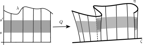
Figure 1. A ruled surface $Q[\eta;\zeta]$ over a geodesic $\zeta$. The shaded region corresponds to $Q_{s}^{s^{\prime}}[\eta;\zeta]$.

Regions inside $Q$: Note that $Q(t,s)$ is at distance $s$ from $\zeta$. Thus, for $0\leq s<s^{\prime}<\operatorname{dist}(\eta,\zeta)$ we can restrict $Q$ to $[0,T]\times[s,s^{\prime}]$ and we denote this by $Q_{s}^{s^{\prime}}[\eta;\zeta]$ or just $Q_{s}^{s^{\prime}}$. Similarly we denote by $Q^{s}$ the level curve $Q$ restricted to $[0,T]\times s$. Note that $Q^{0}$ is a (not necessarily injective) parametrization of $\zeta$.

If $\pi_{\zeta}(\eta)$ is contained in the interior of $\zeta$, and if $\eta$ is smooth, then $Q[\eta;\zeta]$ is smooth and for each $x\in\eta$ the geodesic segment $\overline{x\pi_{\zeta}(x)}$ is orthogonal to $\zeta$. In fact the level curves $Q^{s}$ are orthogonal to the rulings $\overline{x\pi_{\zeta}(x)}$ at all intersection points.

We can define the pullback metric on $Q[\eta;\zeta]$ (or on the parametrizing domain) and denote its Gaussian curvature $\kappa$. We also define the intrinsic geodesic curvature $k_{g}$ along horizontal curves $Q^{s}$ for $s>0$, oriented so that is positive if $Q^{s}$ is curved away from the bottom curve $Q^{0}$. With this convention $-k_{g}$ is non-negative [Mod16, Theorem 4.2]. We let $dm_{s}$ be the measure on the level curve $Q^{s}$ induced by integrating $-k_{g}$. Negative curvature implies that this family of measures is monotonic and weak-$*$ converges to a measure $m$ on $Q^{0}$ [Mod16, Claim 4.3], in particular

$$\int_{Q^{0}}dm=\lim_{s\to 0}\int_{Q^{s}}-k_{g}.$$

This provides the curvature term for the bottom edge of $Q$ which allows us to write a version of the Gauss-Bonnet theorem (this is formula (4.5) in [Mod16, §4.1]):

Theorem 2.18.

(Gauss-Bonnet) Let $Q=Q[\eta;\zeta]$ where $\eta$ is also a geodesic, and let $\theta_{i},\;i=1,2,3,4$ be the exterior angles at the four corners of $Q$. Then

$$\iint_{Q}\kappa dA-\int_{Q^{0}}dm=2\pi-\sum_{i=1}^{4}\theta_{i}.$$

Remark 2.19.

Note that the exterior angles at the bottom corners are $\frac{\pi}{2}$, since we are in the case where the rulings of $Q$ are orthogonal to $\zeta$. However, the internal angles at those corners might be larger than $\frac{\pi}{2}$, which would be accounted for by atomic components of the measure $dm$.

It is helpful to define, for any $Q$,

(2.12) $$\operatorname{\mathcal{I}}(Q)=\iint_{Q}-\kappa dA+\int_{Q^{0}}dm$$

Note that $\operatorname{\mathcal{I}}(Q)\geq 0$ and is monotonic, so that for example if $s\leq dist(\eta,\zeta)$ and $\eta^{\prime}$ is a sub-path of $\eta$, we have

(2.13) $$\operatorname{\mathcal{I}}(Q_{0}^{s}[\eta^{\prime};\zeta])\leq\operatorname{\mathcal{I}}(Q[\eta;\zeta]).$$

Lower bounds on $\operatorname{\mathcal{I}}$

When $\zeta$ is close to the thick part of the stratum of a co-large multicurve, we obtain lower bounds on $\operatorname{\mathcal{I}}(Q)$ for certain ruled surfaces $Q$. Recall large subsurfaces from Definition 2.1. Then, Lemma 6.3 in [Mod16] importing some of the information from the statement of Theorem 5.14 of the paper can be rephrased as follows:

Lemma 2.20.

Let $\bar{\epsilon}>0$ and let $b>0$ be the corresponding constant from Lemma 2.3. Then, for any $d\in(0,b)$ and $e>0$ there exists a $K_{0}>0$ such that the following holds: Let $\sigma$ be a co-large multicurve, and let $\zeta$ be a geodesic segment in $U_{d,\bar{\epsilon}}(\sigma)$ with length at least $1$. Let $Q[\eta;\zeta]$ be a ruled surface with $\operatorname{dist}(\eta,\zeta)>e$. Then

$$\operatorname{\mathcal{I}}(Q_{0}^{e})\geq K_{0}.$$

Proof.

Here we only sketch the proof of the lemma. The detailed analysis, using suitable frame fields introduced by Wolpert [Wol08, §4], and standard properties of Jacobi fields is carried out in $\S 5$ and Lemma 6.3 of [Mod16].

Negative curvature implies that the level sets $Q^{t}$ are expanding with $t$, so that the area of $Q_{0}^{e}$ is bounded below by $e$. Hence the first term in the definition of $\operatorname{\mathcal{I}}(Q_{0}^{e})$ would give the desired lower bound provided that the sectional curvatures (in the planes tangent to $Q$) are bounded away from 0. These sectional curvatures are indeed strictly negative in the thick part of Teichmüller space, as well as, near the stratum of $\sigma$, in the directions nearly tangent to the stratum (this last fact follows from the assumption that $S\smallsetminus\sigma$ is large, hence the stratum has no nontrivial product structure). Thus one may consider, pointwise on $Q$, two cases: if the ruling geodesic direction of $Q$ is nearly tangent to the stratum direction, one obtains a strictly negative curvature bound. If the ruling is transverse to the stratum direction, then in one direction or the other the ruling geodesic exits a neighborhood of the stratum, and enters the regime of strictly negative curvature in all directions. This again gives a definite contribution to the integral. ∎

2.8. Asymptotic rays

In this subsection we prove a result on asymptotic and strongly asymptotic rays that will be useful in Section 4. The first statement of the proposition is a variation on Theorem 6.2 of [Mod16], giving a criterion for promoting asymptoticity to strong asymptoticity in our setting.

(Recall that a ray $r:[0,\infty)\to\operatorname{\mathcal{X}}$ in a metric space is asymptotic to a subset $\operatorname{\mathcal{Y}}\subseteq\operatorname{\mathcal{X}}$ if $\operatorname{dist}(r(t),\operatorname{\mathcal{Y}})$ is bounded above for all $t\in[0,\infty)$. The ray is strongly asymptotic to the subset if $\lim_{t\to\infty}\operatorname{dist}(r(t),\operatorname{\mathcal{Y}})=0$.)

Proposition 2.21.

Let $r$ and $r^{\prime}$ be two asymptotic geodesic rays in $\overline{\operatorname{Teich}(S)}$ such that $r([T,\infty])\subset U_{d,\bar{\epsilon}}(\omega)$ for $d<b$, $T\geq 0$ and a co-large multicurve $\omega$. Then $r$ and $r^{\prime}$ are in fact strongly asymptotic.

For any ray $r$ contained in $\operatorname{\mathcal{S}}_{\bar{\epsilon}}(\omega)$ there is a ray $r_{1}$ in $\operatorname{Teich}(S)$ which is strongly asymptotic to $r$.

Proof.

We begin by proving the first statement in the case where $r$ and $r^{\prime}$ are in the interior, $\operatorname{Teich}(S)$.

Following the notation of $\S$2.7 let $Q$ be the ruled surface $Q[r^{\prime};r]$. Let $\pi_{r}$ denote the nearest point projection to $r$. Since it is continuous, for each $n$ there is an interval $J_{n}$ such that $\pi_{r}(r^{\prime}(J_{n}))=r([0,n])$. Similarly for each $i$ there is an interval $I_{i}$ such that $\pi_{r}(r^{\prime}(I_{i}))=r([i,i+1])$.

Suppose by way of contradiction that the distance from $r^{\prime}(t)$ to $r$ remains bounded below by $e>0$ for all $t$. Then, since $r([i,i+1])\subset U_{d,\bar{\epsilon}}(\omega)$, by Lemma 2.20 we have $\operatorname{\mathcal{I}}(Q_{0}^{e}[r^{\prime}|_{I_{i}},r|_{[i,i+1]}])\geq K_{0}$ for a uniform $K_{0}>0$, and hence

$$\operatorname{\mathcal{I}}(Q[r^{\prime}|_{J_{n}},r|_{[0,n]})\geq K_{0}n.$$

Moreover, by Theorem 2.18 (Gauss-Bonnet) the left-hand side of the above inequality is bounded above by $4\pi$, which implies that $n\leq\frac{4\pi}{K_{0}}$. However $n$ could be chosen arbitrarily large which is a contradiction. Therefore, $r$ and $r^{\prime}$ are strongly asymptotic.

Now we prove the second part. Let $r$ lie in $\operatorname{\mathcal{S}}_{\bar{\epsilon}}(\omega)$, where $\omega$ is co-large. As in the proof of Theorem 1.3 of [BMM10], we fix a basepoint $x\in\operatorname{Teich}(S)$ within $b$ of $r(0)$, let $y_{n}=r(n)$ and use CAT(0) geometry of $\overline{\operatorname{Teich}(S)}$ (via Lemma 8.3 in [BH99, §II.8]) to conclude that the segments $\overline{xy_{n}}$ converge to an infinite ray $r_{1}$ in $\overline{\operatorname{Teich}(S)}$, which is asymptotic to $r$.

We claim that $r_{1}$ is entirely inside $\operatorname{Teich}(S)$. Suppose that $T>0$ is the first time that $r_{1}$ intersects a completion stratum $\operatorname{\mathcal{S}}(\sigma)$. The segment $r_{1}([0,T+1])$ then has at least one endpoint in $\operatorname{Teich}(S)$ and hence by Theorem 2.9 (Nonrefraction) its interior maps to $\operatorname{Teich}(S)$. This contradicts the assumption that $r_{1}(T)\in\operatorname{\mathcal{S}}(\sigma)$.

To see that $r_{1}$ is strongly asymptotic to $r$, for a $\delta>0$ let $x_{\delta}$ be the point on the geodesic segment $\overline{r(0)r_{1}(0)}$ at distance $\delta$ from $r(0)$. (it must be in $\operatorname{Teich}(S)$ by Theorem 2.9). Let $r_{\delta}$ be the geodesic obtained as above as the limit of $\overline{x_{\delta}y_{n}}$. As we saw above $r_{\delta}$ is an infinite ray in $\operatorname{Teich}(S)$ which remains in a $\delta$-neighborhood of $r$ and in particular in $U_{\delta,\bar{\epsilon}}(\omega)$. Since the rays $r_{\delta}$ and $r_{1}$ are asymptotic and in $\operatorname{Teich}(S)$, the first part of the proposition implies (for sufficiently small $\delta$) that $r_{1}$ and $r_{\delta}$ are in fact strongly asymptotic. Letting $\delta\to 0$, the strong asymptoticity of $r_{1}$ to $r$ follows.

Finally, we prove the first part of the proposition in the general case. Using the second part, $r$ and $r^{\prime}$ are strongly asymptotic to $r_{1}$ and $r^{\prime}_{1}$ respectively, which lie in the interior. The version of first part that we already proved shows that $r_{1}$ and $r^{\prime}_{1}$ are strongly asymptotic, and this concludes the proof. ∎

3. Non-annular bounded combinatorics

In this section we study the case that the end invariant of a WP geodesic satisfies the non-annular bounded combinatorics condition:

Definition 3.1.

(Bounded combinatorics) We say that a pair of markings or laminations $(\mu,\mu^{\prime})$ satisfies $R$–bounded combinatorics if

$$d_{Y}(\mu,\mu^{\prime})\leq R$$

for all proper subsurfaces $Y\subsetneq S$. If the bound holds for non-annular proper subsurfaces, we say the pair satisfies non-annular $R$–bounded combinatorics.

When the end invariant of a WP geodesic satisfies non-annular bounded combinatorics, the short curves correspond exactly to the annulus with big subsurface coefficients. More precisely:

Theorem 3.2.

For any $R,\epsilon_{0}>0$ there are functions $\hat{N}:\operatorname{\mathbb{R}}_{>0}\to\operatorname{\mathbb{R}}_{>0}$ and $\hat{\epsilon}:\operatorname{\mathbb{R}}_{>0}\to\operatorname{\mathbb{R}}_{>0}$ such that the following holds.

Suppose that $g$ is a WP geodesic with end invariant $(\nu^{+},\nu^{-})$, where $\nu^{\pm}$ are either laminations in $\operatorname{\mathcal{EL}}(S)$ or points in the $\epsilon_{0}$-thick part, which satisfy non-annular $R$–bounded combinatorics. Then

1. for any $N\geq 1$, if $\inf_{t}\ell_{\gamma}(g(t))<\hat{\epsilon}(N)$ then $d_{\gamma}(\nu^{-},\nu^{+})\geq N$.

2. for any $\epsilon>0$, if $d_{\gamma}(\nu^{-},\nu^{+})\geq\hat{N}(\epsilon)$ then $\inf_{t}\ell_{\gamma}(g(t))<\epsilon$.

Proof.

Let $\rho:I\to\operatorname{\mathcal{P}}(S),\;I\subseteq\operatorname{\mathbb{R}}\cup\{\pm\infty\}$, be a hierarchy path in the pants graph of $S$ that connects the points $\nu^{-}$ and $\nu^{+}$; see §2.3. Let $Q:\operatorname{Teich}(S)\to\operatorname{\mathcal{P}}(S)$ be Brock’s (see (2.3)). The non-annular $R$–bounded combinatorics property implies, via [BMM11, Theorem 4.4] (also [Mod15, Theorem 5.13]), that $Q\circ g$ and $\rho$ are $D$–fellow-travelers in $\operatorname{\mathcal{P}}(S)$, where $D$ is a constant depending only on $R$. Moreover, the non-annular $R$-bounded combinatorics condition together with the distance formula (2.4) implies that condition (2.9) in Theorem 2.17 holds with the whole surface $S$ playing the role of $X$. That is,

$$d_{\operatorname{\mathcal{P}}}(\rho(i),\rho(j))\asymp_{K,C}d_{S}(\rho(i)),\rho(j))$$

with constants $K,C$ depending only on $R$.

Proof of part (1):

Given $\epsilon>0$ and less than the Bers constant $L_{S}$, suppose for some $t\in\operatorname{\mathbb{R}}$ that $\ell_{\gamma}(g(t))<\epsilon$. Then $\gamma$ is in a Bers pants decomposition $Q(g(t))$ at $g(t)$, and by the fellow traveling of $Q(g)$ and $\rho$, $Q(g(t))$ is within distance $D$ of $\rho(i)$ for some $i\in I$.

Let $w,B>0$ be the constants provided by Theorem 2.17. Then let $t_{1},t_{2}$ be so that the pants decompositions $Q(g(t_{1}))$, $Q(g(t_{2}))$ are within distance $D$ of $\rho(i-w)$ and $\rho(i+w)$, respectively, then the inequality (2.10) from the theorem gives us

(3.1) $$\Big{|}d_{\gamma}\left(Q(g(t_{1})),Q(g(t_{2}))\right)-d_{\gamma}\left(\rho(i-w),\rho(i+w)\right)\Big{|}\leq 2B.$$

Moreover, by (2.11) from the theorem we have that:

(3.2) $$\min\{\ell_{\gamma}(g(t_{1})),\ell_{\gamma}(g(t_{2}))\}>\omega.$$

Now, note that the length of $[t_{1},t_{2}]$ is bounded independently of $g$ and $t$ with a constant that depends only on $R$ and $D$. Thus we can apply Theorem 2.13 to the geodesic segment $g|_{[t_{1},t_{2}]}$ to conclude that, for any $N\in\operatorname{\mathbb{N}}$, there is an $\epsilon<\min\{\omega,L_{S}\}$, so that if $\inf_{t\in[t_{1},t_{2}]}\ell_{\gamma}(g(t))<\epsilon$, then

$$d_{\gamma}(Q(g(t_{1})),Q(g(t_{2})))\geq N+2B+M,$$

where the constant $M$ is from Proposition 2.4 (no-backtracking). By the inequality (3.1) this implies that

$$d_{\gamma}(\rho(i-w),\rho(i+w))\geq N+M.$$

Then by Proposition 2.4 we have

$$d_{\gamma}(\nu^{-},\nu^{+})\geq N$$

which concludes the proof of part (1).

Proof of part (2):

By [MM00, Lemma 6.2] if $d_{\gamma}(\nu^{-},\nu^{+})\geq N$ where $N\in\operatorname{\mathbb{N}}$ is larger than a threshold, the curve $\gamma$ appears as a curve in a pants decomposition $\rho(i)$ where $i\in I$. Then similar to part (1) by Theorem 2.17 there are constants $w,B>0$ and $\omega>0$, so that the inequalities (3.1) and (3.2) hold.

Moreover, appealing again to the no-backtracking property of hierarchy paths, we have

$$d_{\gamma}(\rho(i-w),\rho(i+w))\geq N-M.$$

The fellow-traveling property of $\rho$ and $Q(g)$ guarantees that there are $t_{1},t_{2}$ so that $Q(g(t_{1}))$ and $Q(g(t_{2}))$ are within distance $D$ of $\rho(i-w)$ and $\rho(i+w)$ respectively. So by (3.1) we have

$$d_{\gamma}(Q(g(t_{1})),Q(g(t_{2})))\geq N-M-2B.$$

Also, the length of the interval $[t_{1},t_{2}]$ is bounded independently of $g$, thus appealing to Theorem 2.11, for any $\epsilon>0$, there is an $N\in\operatorname{\mathbb{N}}$ so that

$$\inf_{t\in[t_{1},t_{2}]}\ell_{\gamma}(g(t))<\epsilon,$$

which gives us part (2) of the theorem. ∎

4. Bottlenecks and visibility

The main result of this section is Theorem 1.2 on existence of bottlenecks, which we restate here:

Theorem 1.2. Let $\omega,\omega^{\prime}$ be two co-large multicurves that fill $S$. Let $\bar{\epsilon}>0$ and let $r$ and $r^{\prime}$ be infinite length WP geodesic rays in $\overline{\operatorname{Teich}(S)}$ that are strongly asymptotic to (or contained in) the $\bar{\epsilon}$–thick parts of the strata $\operatorname{\mathcal{S}}(\omega)$ and $\operatorname{\mathcal{S}}(\omega^{\prime})$, respectively. Then $r$ and $r^{\prime}$ have a bottleneck.

As a consequence of the above theorem we will also obtain a visibility theorem, which is Theorem 4.5 stated in Subsection 4.2.

We start with the following observations about the rays $r$ and $r^{\prime}$:

Lemma 4.1.

The rays $r$ and $r^{\prime}$ diverge; that is

$$\lim_{t\to\infty}\operatorname{dist}(r^{\prime}(t),r)=\infty$$

and the corresponding statement holds when interchanging $r$ and $r^{\prime}$.

Proof.

The lemma would follow once we show that, for any $R>0$, the intersection of $R$–neighborhoods $\operatorname{\mathcal{N}}_{R}(\operatorname{\mathcal{S}}(\omega))\cap\operatorname{\mathcal{N}}_{R}(\operatorname{\mathcal{S}}(\omega^{\prime}))$ has finite diameter.

To see this fact, we start with a consequence of the distance formula (2.5):

(4.1) $$\operatorname{dist}(x,\operatorname{\mathcal{S}}(\omega))\asymp\sum_{\begin{subarray}{c}Y\subseteq S:\;\operatorname{na},\;\omega\pitchfork Y\end{subarray}}\{d_{Y}(x,\omega)\}_{A}$$

with constants that depend only on $A$. This follows by checking that, for any $y\in\operatorname{\mathcal{S}}(\omega)$ minimizing pants distance to $x$, the projections to subsurfaces in the complement of $\omega$ do not contribute to the sum. The argument appears, in a slightly different context, in Proposition 3.1 of [BKMM12].

Now if $x\in\operatorname{\mathcal{N}}_{R}(\operatorname{\mathcal{S}}(\omega))\cap\operatorname{\mathcal{N}}_{R}(\operatorname{\mathcal{S}}(\omega^{\prime}))$ we apply (4.1) to both $\omega$ and $\omega^{\prime}$. Since $\omega\cup\omega^{\prime}$ fills $S$, every $Y\subseteq S$ intersects $\omega$ or $\omega^{\prime}$, so we obtain an upper bound independent of $x$ for

$$\sum_{\begin{subarray}{c}Y\subseteq S:\;\operatorname{na}\end{subarray}}\{d_{Y}(x,\omega\cup\omega^{\prime})\}_{A}.$$

But since $\omega\cup\omega^{\prime}$ is a fixed collection of curves this gives a uniform upper bound on $d(x,x_{0})$ for a fixed basepoint $x_{0}$ and all $x\in\operatorname{\mathcal{N}}_{R}(\operatorname{\mathcal{S}}(\omega))\cap\operatorname{\mathcal{N}}_{R}(\operatorname{\mathcal{S}}(\omega^{\prime}))$. This gives the desired diameter bound. ∎

For the rest of the proof let us assume that $r$ and $r^{\prime}$ are in the interior $\operatorname{Teich}(S)$. At the end we will derive the full statement.

4.1. The ruled triangle argument

Let $u=r(0)$ and $u^{\prime}=r^{\prime}(0)$. We will show that for any two points $p$ on $r$ and $q$ on $r^{\prime}$ the geodesic segment $\overline{pq}$ meets a compact subset of Teichmüller space. The first ingredient of the proof is the following:

Lemma 4.2.

The distance $\operatorname{dist}(u,\overline{pq})$ is bounded independently of $p$ and $q$.

Proof.

Let $\zeta$ denote the composed path $\overrightarrow{uq}*\overrightarrow{qp}$. Then let $Q=Q[\zeta;r]$ be the ruled surface over $r$ parametrized by $\zeta$ (as defined in §2.7).

Let $b>0$ be the constant from Lemma 2.3 corresponding to $\bar{\epsilon}>0$, and let $J\subset\zeta$ be the subset of $\zeta$ at distance greater than $b/2$ from $r$ i.e.

(4.2) $$J:=\{v\in\zeta:d(v,r)\geq b/2\}.$$

By convexity of the distance function in a CAT(0) metric the interval $J$, if nonempty, is an interval containing the apex $q$ of the geodesic triangle $\triangle uqp$.

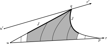
Figure 2. The ruled triangle $Q[\zeta;r]$ determined by $u,p,q$. The ruled subsurface $Q[J;r]$ is shaded.

Claim 4.3.

There is a bounded interval $I$ of $r$ containing $\pi_{r}(J)$ for any $p,q$.

To see this, we first show that the left endpoint of $\pi_{r}(J)$ is a bounded distance from $u$.

We know from Lemma 4.1 that $\operatorname{dist}(r^{\prime}(t),r)\to\infty$. Thus let $t_{0}$ be such that $t>t_{0}$ implies $\operatorname{dist}(r^{\prime}(t),r)>b/2+D$, where $D=d(u,u^{\prime})$. Now if $y\in\overline{uq}$ with $d(y,u)>t_{0}+2D$, let $y^{\prime}\in r^{\prime}$ be such that $d(y,y^{\prime})\leq D$. Note that such a $y^{\prime}$ exists from the CAT(0) comparison for the triangle $\triangle uu^{\prime}q$. Then $d(y^{\prime},u^{\prime})>t_{0}$, so $d(y^{\prime},r)>b/2+D$. We conclude that $d(y,r)>b/2$. Hence the left endpoint of $J$ must be at most distance $t_{0}+2D$ apart from $u$, which means the left endpoint of $\pi_{r}(J)$ is at most distance $t_{0}+2D+b/2$ apart from $u$.

Next, we prove that the length of $\pi_{r}(J)$ is bounded. Let $d\in(0,b/2)$ be small enough (say less than $b/4$) and let $K_{0}>0$ be the constant from Lemma 2.20 corresponding to $e=b/2,\bar{\epsilon}$ and $d$. Let $T>0$ be such that $r([T,\infty))$ is contained in $U_{d,\bar{\epsilon}}(\omega)$, which is possible by the hypothesis that $r$ is strongly asymptotic to the $\bar{\epsilon}$–thick part of $\operatorname{\mathcal{S}}(\omega)$.

If $\pi_{r}(J)$ has length greater than $n+1+T$, then there exist $n$ disjoint intervals of length $1$, $I_{i},\;i=1,\ldots,n$ in the interior of $\pi_{r}(J)$ and in $U_{d,\bar{\epsilon}}(\omega)$. For $i=1,\ldots,n$ let $J_{i}$ be the subinterval of $J$ whose $\pi_{r}$-image is the interval $I_{i}$. We may choose the $I_{i}$ so that each $J_{i}$ is disjoint from $q$ (possibly discarding one if necessary). Then $Q$ contains the regions $Q[J_{i};r]$, and each of these contains a subrectangle $Q_{0}^{b/2}[J_{i};r]$. From Lemma 2.20 then we have

$$\operatorname{\mathcal{I}}(Q_{0}^{b/2}[J_{i};r])\geq K_{0}$$

where $K_{0}$ depends only on $b$ and $\bar{\epsilon}$.

Thus by the monotonicity of $\operatorname{\mathcal{I}}$ (2.13), $\operatorname{\mathcal{I}}(Q)\geq nK_{0}$. However, $\operatorname{\mathcal{I}}(Q)$ is controlled by the Gauss-Bonnet theorem (Theorem 2.18), which in this case gives $\operatorname{\mathcal{I}}(Q)\leq\pi$. This bounds $n$, and hence the length of $\pi_{r}(J)$, giving Claim 4.3.

The right endpoint of $\pi_{r}(J)$, then is a bounded distance from $u$ and at distance $b/2$ from $\overline{pq}$. This proves the lemma. ∎

Proof of Theorem 1.2.

The proof will reduce easily to the following statement:

Lemma 4.4.

There is a compact subset $K_{1}\subsetneq\operatorname{Teich}(S)$ so that, for points $p\in r,q\in r^{\prime}$ sufficiently far out, the segment $\overline{pq}$ intersects $K_{1}$.

Proof.

The proof of Lemma 4.2 actually gave us a point $\hat{z}$ on $\overline{pq}$ such that $d(\hat{z},r)\leq b/2$ (the right end point of $J$). Then since $r$ is strongly asymptotic to $\operatorname{\mathcal{S}}_{\bar{\epsilon}}(\omega)$, moving $\hat{z}$ along $\overline{pq}$ toward $p$ a bounded distance we obtain a point $z\in\overline{pq}$, and the point $y=\pi_{r}(z)$ on $r$, such that:

1. $d(y,\operatorname{\mathcal{S}}_{\bar{\epsilon}}(\omega))<b/4$

2. $d(z,y)\leq b/2$

3. $d(z,\hat{z})>1$

4. $d(z,u)$ is bounded independently of $p$ and $q$.

We can similarly move $\hat{z}$ toward $q$ to obtain $z^{\prime}$ and $y^{\prime}=\pi_{r^{\prime}}(z^{\prime})$ so that the inequalities (1)-(4) hold for the points $u^{\prime},y^{\prime},z^{\prime}$ and the multicurve $\omega^{\prime}$. Thus the geodesic hexagon $H$ joining the vertices

$$u^{\prime},u,y,z,z^{\prime},y^{\prime}$$

in cyclic order has bounded total length independently of $p$ and $q$ (Figure 3).

Figure 3. The bounded diameter hexagon $H$ determined by $u^{\prime},u,y,z,z^{\prime},y^{\prime}$.

We will next show that

• $d_{\alpha}(z,z^{\prime})$ is bounded above for each curve $\alpha$, by a quantity independent of $\alpha$, $p$ and $q$, and

• $\ell_{\alpha}$ is bounded below on $\overline{zz^{\prime}}$ by a positive constant independent of $\alpha$, $p$ and $q$.

Fix any curve $\alpha$. Since the multicurves $\omega$ and $\omega^{\prime}$ fill $S$, $\alpha$ must intersect at least one of them. Suppose that $\alpha\pitchfork\omega$. Then we have the following uniform bounds (all independent of $p$, $q$ and $\alpha$) for the $\alpha$ coefficients:

1. $d_{\alpha}(u,u^{\prime})$ is uniformly bounded; because the points $u,u^{\prime}$ are fixed.

2. $d_{\alpha}(u,y)$ is uniformly bounded; this is because $y$ varies along a compact interval in $r$. To see that the bound is independent of $\alpha$, note that the set of Bers markings that can occur for values of $y$ in this interval is finite, and the set of $\alpha$ with $d_{\alpha}(u,\mu)$ large for any given marking $\mu$ is finite, by an application of the distance formula (2.4).

3. $d_{\alpha}(y,z)$ is uniformly bounded; by inequalities (1) and (2), we have that $\overline{yz}$ is in $U_{b,\bar{\epsilon}}(\omega)$. Within this neighborhood there is an upper bound on the length of $\omega$, and since $\alpha\pitchfork\omega$ this means that $\pi_{\alpha}(\overline{yz})$ is uniformly close to $\pi_{\alpha}(\omega)$.

Now further suppose that $\alpha\notin\omega^{\prime}$. Then we have the bounds:

1. $d_{\alpha}(u^{\prime},y^{\prime})$ is uniformly bounded; this follows just as in (ii) above.

2. $d_{\alpha}(y^{\prime},z^{\prime})$ is uniformly bounded; since $\overline{y^{\prime}z^{\prime}}$ is in $U_{b,\bar{\epsilon}}(\omega^{\prime})$ and $\alpha\notin\omega^{\prime}$ the bound may be obtained similarly to (iii). Here, while $\alpha$ may not intersect $\omega^{\prime}$, it does intersect curves in $S\smallsetminus\omega^{\prime}$ whose lengths can only vary by a bounded amount in $\overline{y^{\prime}z^{\prime}}$ because $S\smallsetminus\omega^{\prime}$ is uniformly thick along $\overline{y^{\prime}z^{\prime}}$ by Lemma 2.3.

Combining (i)-(iii) and (a) and (b), we obtain a uniform bound on $d_{\alpha}(z,z^{\prime})$ for all curves $\alpha$ such that $\alpha\pitchfork\omega$ and $\alpha\notin\omega^{\prime}$, and all $p\in r$ and $q\in r^{\prime}$.

Now since $z\in U_{\bar{\epsilon},b}(\omega)$ and $z^{\prime}\in U_{\bar{\epsilon},b}(\omega^{\prime})$, there is a positive lower bound for the length of any $\alpha$ as above at the points $z$ and $z^{\prime}$ by Lemma 2.3. Combining this with the bound for $d_{\alpha}(z,z^{\prime})$ and appealing to Theorem 2.13, we obtain a uniform positive lower bound for the length of $\alpha$ along $\overline{zz^{\prime}}$.

Now suppose that $\alpha\pitchfork\omega$ and $\alpha\in\omega^{\prime}$. First we show that $\ell_{\alpha}$ is uniformly bounded below on $\overline{zz^{\prime}}$. If not, we can fix $\alpha$ among the finitely many choices, and obtain a sequence of segments $\{\overline{p_{n}q_{n}}\}_{n}$ with subsegments $\overline{z_{n}z^{\prime}_{n}}$, and $x_{n}\in\overline{z_{n}z^{\prime}_{n}}$ such that $\ell_{\alpha}(x_{n})\to 0$ as $n\to\infty$. We may assume that $q_{n}$ goes to $\infty$ along $r^{\prime}$.

Now since $q_{n}$ goes to infinity along $r^{\prime}$, and $r^{\prime}$ is strongly asymptotic to $\operatorname{\mathcal{S}}_{\bar{\epsilon}}(\omega^{\prime})$, we have $\ell_{\alpha}(q_{n})\to 0$ as $n\to\infty$. Convexity of length-functions then implies that the length of $\alpha$ goes to $0$ uniformly along $\overline{x_{n}q_{n}}$. Thus we may find subintervals $\eta_{n}$ of $\overline{p_{n}q_{n}}$ of fixed length, centered at $x_{n}$ so that the length of $\alpha$ goes to 0 on one side of $x_{n}$ and is bounded away from 0 on the opposite endpoint of $\eta_{n}$. This contradicts Lemma 2.10. Thus we obtain the desired lower bound for the length of $\alpha$.

Now we show that $d_{\alpha}(z,z^{\prime})$ is uniformly bounded. If not, again we can fix $\alpha$ among the finitely many choices, and obtain a sequence of segments $\{\overline{p_{n}q_{n}}\}_{n}$ with subsegments $\overline{z_{n}z^{\prime}_{n}}$ such that $d_{\alpha}(z_{n},z^{\prime}_{n})\to\infty$ as $n\to\infty$.

Since $z_{n}\in U_{b,\bar{\epsilon}}(\omega)$ and $\alpha\pitchfork\omega$, again by Lemma 2.3 $\ell_{\alpha}(z_{n})$ is bounded below by a positive constant for all $n$. Moreover, the lengths of $\overline{z_{n}z^{\prime}_{n}}$ are bounded below by (3) and bounded above by (4) independently of $n$. Thus we may apply Theorem 2.11 to see that after possibly passing to a subsequence there is a point $x_{n}\in\overline{z_{n}z^{\prime}_{n}}$ such that $\ell_{\alpha}(x_{n})\to 0$ as $n\to\infty$. But then as we saw above this leads to a contradiction, showing that $d_{\alpha}(z,z^{\prime})$ must be uniformly bounded above.

Thus we obtain both (*) and (**) for all $\alpha\pitchfork\omega$. The case of $\alpha\pitchfork\omega^{\prime}$ proceeds similarly, exchanging the roles of $\omega$ and $\omega^{\prime}$.

With (**) established, we conclude that $\overline{zz^{\prime}}$ lies in the $\varepsilon$-thick part of $\operatorname{Teich}(S)$, for $\varepsilon>0$ independent of $p$ and $q$. Since there is an upper bound on the ratio of Teichmüller norm over WP norm in the $\varepsilon$-thick part, and the WP length of $\overline{zz^{\prime}}$ is bounded above by (4), we conclude that $\overline{zz^{\prime}}$ has bounded Teichmüller length, and hence $d_{\alpha}(m,z)$ and $d_{\alpha}(m,z^{\prime})$ are uniformly bounded above for any $m\in\overline{zz^{\prime}}$.

Now when $\alpha\pitchfork\omega$ we extract an upper bound for $d_{\alpha}(u,z)$ from (ii-iii), and when $\alpha\pitchfork\omega^{\prime}$ we similarly extract an upper bound for $d_{\alpha}(u,z^{\prime})$ from the analogues of (i-iii). Putting these bounds together we obtain a uniform upper bound for $d_{\alpha}(u,m)$ for all $m\in\overline{zz^{\prime}}$.

We claim now that this implies that $m$ (and hence all of $\overline{zz^{\prime}}$) must remain in some compact subset $K_{1}$ of $\operatorname{Teich}(S)$. For we have an upper bound on $d(u,m)$ by the bounds on the hexagon $H$, and by Lemma 2.13, a sequence of segments $\overline{um}$ (for varying $p,q$) degenerates only by producing arbitrary large twistings about a collection of curves, which is impossible by the bounds we just established on all $d_{\alpha}(u,m)$. Thus $\overline{um}$ has a uniformly bounded length and remains in some thick part of $\operatorname{Teich}(S)$ (independently of $p,q$), so again has uniformly bounded Teichmüller length. But balls in the Teichmüller metric are compact and this gives us $K_{1}$. ∎

From the lemma we obtain points $\hat{p}\in r,\hat{q}\in r^{\prime}$ so that all geodesics with end points $p,q$ on $r,r^{\prime}$, further out than $\hat{p},\hat{q}$ respectively, intersect $K_{1}$. Now letting $K$ be the union of $K_{1}$ and the segments $\overline{u\hat{p}}$ and $\overline{u^{\prime}\hat{q}}$, we have the desired bottleneck. This concludes the proof in the case that $r,r^{\prime}\subset\operatorname{Teich}(S)$.

If $r$ is in $\operatorname{\mathcal{S}}_{\bar{\epsilon}}(\omega)$, using Proposition 2.21 we can find $r_{1}$ in $\operatorname{Teich}(S)$ strongly asymptotic to it, and similarly $r^{\prime}_{1}$ strongly asymptotic to $r^{\prime}$. The interior version of the theorem gives a compact bottleneck $K$ for $r_{1},r^{\prime}_{1}$. There exists $\delta_{1}>0$ so that the $\delta_{1}$-neighborhood of $K$ is still contained in a compact set $K_{2}\subset\operatorname{Teich}(S)$. Now choose $T$ sufficiently large that $d(r(t),r_{1}(t))$ and $d(r^{\prime}(t),r^{\prime}_{1}(t))$ are less than $\delta_{1}$ for all $t>T$. Thus any geodesic $\gamma$ joining $r(t)$ and $r^{\prime}(s)$ for $t,s>T$ lies within $\delta_{1}$ of a geodesic passing through $K$, and hence passes through $K_{2}$. ∎

4.2. Visibility

In this subsection we apply the Bottleneck theorem (Theorem 1.2) to show that any two geodesic rays that are strongly asymptotic to the $\bar{\epsilon}$–thick parts of two strata determined by two filling co-large multicurves have the visibility property.

Theorem 4.5.

(Asymptotic Large Visibility) Suppose $r,r^{\prime}$ are two infinite rays in $\overline{\operatorname{Teich}(S)}$ that are strongly asymptotic to, or contained in, $\operatorname{\mathcal{S}}_{\bar{\epsilon}}(\omega)$ and $\operatorname{\mathcal{S}}_{\bar{\epsilon}}(\omega^{\prime})$, respectively, where $\omega$ and $\omega^{\prime}$ are co-large multicurves that fill $S$. Then there exists a biinfinite geodesic $g\subsetneq\operatorname{Teich}(S)$ which is strongly asymptotic to $r$ in forward time and is strongly asymptotic to $r^{\prime}$ in backward time.

Proof.

The argument is essentially the same as in Theorem 1.3 of [BMM10], which obtains the visibility property when $r$ and $r^{\prime}$ are recurrent. We sketch here the mild changes needed in our setting.

Let $g_{n}$ denote the geodesic segment $\overline{r(n)r^{\prime}(n)}$. By Theorem 1.2 there is a compact set $K\subsetneq\ Teich(S)$ so that $g_{n}\cap K\neq\emptyset$.

Let $v_{n}$ be a point of $g_{n}\cap K$. After possibly passing to a subsequence the points $v_{n}$ converge to a point $v\in K$.

Reparametrize $g_{n}$ so that $g_{n}(0)=v_{n}$. To extract a limit of the $g_{n}$ we use the CAT(0) geometry of $\overline{\operatorname{Teich}(S)}$, via Lemma 8.3 in [BH99, §II.8], together with the fact that $g_{n}(0)\to v$, to show that for each $t\in\operatorname{\mathbb{R}}$ the sequence $g_{n}(t)$ (defined for large $n$) is a Cauchy sequence. We thus obtain a limiting geodesic $g$ in $\overline{\operatorname{Teich}(S)}$, which is asymptotic to $r$ in forward time and to $r^{\prime}$ in backward time.

As in [BMM10] and Proposition 2.21, we use the non-refraction property (Theorem 2.9) to argue that $g$ is in fact contained in $\operatorname{Teich}(S)$.

Finally, Proposition 2.21 implies that $g$ is strongly asymptotic to $r$ in forward time and $r^{\prime}$ in backward time. ∎

5. Indirect shortening along geodesic segments

This section is devoted to the proof of Theorem 1.3, which follows very directly from Theorem 5.5 below. We begin with a discussion of the phenomenon of indirect shortening.

5.1. Indirect curve shortening

In the setting of Teichmüller geodesics the connection between short curves and large subsurface coefficients was explored by Rafi in [Raf05]. He showed that given $\epsilon>0$ there exists $A\geq 1$ so that, if $g:I\to\operatorname{Teich}(S)$ is a Teichmüller geodesic with end invariant $(\nu^{+},\nu^{-})$, then for any subsurface $Z\subseteq S$ we have

$$d_{Z}(\nu^{+},\nu^{-})\geq A\implies\inf_{t}\ell_{\partial Z}(g(t))<\epsilon.$$

The natural converse statement, which is motivated by the situation for Kleinian surface groups (see Theorem 7.1), would be that given $A\geq 1$ there exists $\epsilon>0$ such that, if a curve $\gamma$ satisfies

$$\inf_{t}\ell_{\gamma}(g(t))<\epsilon$$

then there exists a subsurface $Z$ with $\gamma\subseteq\partial Z$, and

$$d_{Z}(\nu^{+},\nu^{-})\geq A.$$

This converse, however, does not hold in general. Rafi in the proof of Theorem 1.7 in [Raf05] gave and analyzed examples of sequences of geodesic segments $g_{n}$ with end invariants $(\nu^{+}_{n},\nu^{-}_{n})$ and a curve $\gamma$ for which $\inf_{t}\ell_{\gamma}(g_{n}(t))$ is arbitrarily small, while $d_{Z}(\nu^{+}_{n},\nu^{-}_{n})$ remains bounded for all $Z\subseteq S$ with $\gamma\subseteq\partial Z$.

Rafi’s examples exhibited a somewhat more complex feature we might call indirect shortening. To present the example we start with two definitions:

Definition 5.1.

Given $A\geq 1$, a subsurface $Z\subseteq S$ and a pair of markings or laminations $(\mu,\mu^{\prime})$ we define

$$\operatorname{\mathcal{L}}_{A}(Z,\mu,\mu^{\prime}):=\{X\subseteq Z:d_{X}(\mu,\mu^{\prime})>A\}.$$

We define $\operatorname{\mathcal{L}}^{\operatorname{na}}_{A}(Z,\mu,\mu^{\prime})$ as the subset of non-annular surfaces in $\operatorname{\mathcal{L}}_{A}(Z,\mu,\mu^{\prime})$.

Definition 5.2.

(Filling a subsurface) Let $Z\subseteq S$, we say that a collection $\operatorname{\mathcal{Z}}$ of subsurfaces of $Z$ fills $Z$ if any curve $\alpha\in\operatorname{\mathcal{C}}(Z)$ intersects at least one $X\in\operatorname{\mathcal{Z}}$ essentially.

In fact, Rafi in [Raf05, §6] gave examples of geodesics $g$ with the following property:

Definition 5.3.

(Indirect curve shortening) Given $\epsilon>0$ and $A\geq 1$, $\inf_{t}\ell_{\gamma}(g(t))<\epsilon$ and there exists a subsurface $Z$ with $\gamma\subseteq\partial Z$ that $\operatorname{\mathcal{L}}_{A}(Z,\nu^{+},\nu^{-})$ fills $Z$, but $Z\notin\operatorname{\mathcal{L}}_{A}(Z,\nu^{+},\nu^{-})$.

We call the property indirect curve shortening because the subsurface $Z$ itself does not have a big projection coefficient.

More recently it has become clear that this condition, also, does not hold for Teichmüller geodesics in general; see [MR18]. Nevertheless let us state as a conjecture the following characterization for short curves of Weil-Petersson geodesics.

Conjecture 5.4.

For any $\epsilon>0$, there exists $A(\epsilon)\geq 1$, and for any $A\geq 1$ there exists $\epsilon(A)>0$, such that the following holds. Let $g:I\to\operatorname{Teich}(S)$ be a WP geodesic with end invariant $(\nu^{+},\nu^{-})$,

1. If $Z$ is a non-annular subsurface for which $\operatorname{\mathcal{L}}^{\operatorname{na}}_{A(\epsilon)}(Z,\nu^{-},\nu^{+})$ fills $Z$ or $Z$ is an annulus with $d_{Z}(\nu^{+},\nu^{-})>A(\epsilon)$, then $\inf_{t}\ell_{\partial Z}(g(t))<\epsilon$.

2. If $\inf_{t}\ell_{\alpha}(g(t))<\epsilon(A)$ for a curve $\alpha$, then either there exists a subsurface $Z$ with $\alpha\in\partial Z$ such that $\operatorname{\mathcal{L}}^{\operatorname{na}}_{A}(Z,\nu^{+},\nu^{-})$ fills $Z$, or $d_{\alpha}(\nu^{+},\nu^{-})>A$.

5.2. The basic example

To set the stage for our example of WP geodesics with indirect curve shortening property, consider the configuration of subsurfaces of $S$:

(5.1)

where we assume $Z$ is large in $S$, and $X_{j}$ is large in $Z$ for $j=1,2$. We moreover assume that $\partial X_{1}$ and $\partial X_{2}$ fill $Z$ and that no boundary curve of $X_{j}$ is a boundary curve of $Z$ for $j=1,2$. We call this a one-step large filling configuration; see Figure 4 for an example.

Figure 4. One-step large filling: The subsurface $Z$ is a two-holed torus. In its abelian cover on the left we indicate two arcs $a_{1},a_{2}$ connecting the components of $\partial Z$ which fill $Z$. A regular neighborhood of $a_{i}\cup\partial Z$ is a three-holed sphere $U_{i}$, and we define $X_{i}=Z\smallsetminus U_{i}$. Note that $\partial X_{i}$ and $\partial Z$ have no components in common. On the right we indicate $Z$ as a subset of $S$.

We can now state the main theorem of Section 5. The proof will follow over the next few subsections.

Theorem 5.5.

There exist $A_{1}\geq 1,\epsilon_{0}>0$ such that for each $\epsilon>0$ and a one-step large filling configuration $Z,X_{1},X_{2}$, there is a Weil-Petersson geodesic segment $\overline{pq}$ in $\operatorname{Teich}(S)$ such that

• $\operatorname{\mathcal{L}}^{\operatorname{na}}_{A_{1}}(S,p,q)=\{X_{1},X_{2}\}$, and $d_{\gamma}(p,q)\leq 1$ for all $\gamma\subseteq\partial Z$,

• The endpoints $p,q$ are in the $\epsilon_{0}$–thick part of $\operatorname{Teich}(S)$, and

• $\inf_{x\in\overline{pq}}\ell_{\partial Z}(x)<\epsilon$.

5.3. Using visibility in a stratum

Fix for the rest of the section a one-step large filling configuration $Z,X_{1},X_{2}$ in $S$.

Since $Z$ is large the stratum $\operatorname{\mathcal{S}}(\partial Z)$ can be identified with $\operatorname{Teich}(Z)$ after replacing boundary curves with punctures, and similarly the strata of $\partial X_{i}$ within this stratum, namely $\operatorname{\mathcal{S}}(\partial X_{i})\cap\operatorname{\mathcal{S}}(\partial Z)$, can be identified with $\operatorname{Teich}(X_{i})$ for $i=1,2$. Let $f_{1}$ and $f_{2}$ be partial pseudo-Anosov maps supported in $X_{1}$ and $X_{2}$ respectively, so that their axes $g_{1}$ and $g_{2}$ lie in the $\epsilon$-thick part of $\operatorname{Teich}(X_{i})$ for some $\bar{\epsilon}>0$. Fix rays $g_{2}^{+}$ and $g_{1}^{-}$ on these axes.

We can apply Theorem 4.5, with $Z$ playing the role of $S$ in that theorem, to obtain a biinfinite geodesic $h$ in $\operatorname{Teich}(Z)$ asymptotic to the rays $g_{1}^{-}$ in backward time and $g_{2}^{+}$ in forward time.

The geodesic segment examples for Theorem 5.5 will be obtained from $h$, viewed in $\operatorname{\mathcal{S}}(\partial Z)$, by pushing points far out along $h$ slightly away from the stratum. The key will then be to show that, for these geodesics, the subsurface coefficients behave as required, and the length of $\partial Z$ becomes very small near the center.

5.4. Controlling subsurface coefficients along $h$

Recall that $g_{1}$ and $g_{2}$ are geodesics in the $\bar{\epsilon}$–thick parts of $\operatorname{Teich}(X_{1})$ and $\operatorname{Teich}(X_{2})$, respectively, and let $b>0$ be the corresponding constant to $\bar{\epsilon}$ from Lemma 2.3.

Let us fix a parametrization of the bi-infinite geodesic $h:\operatorname{\mathbb{R}}\to\operatorname{Teich}(Z)$ and of the geodesics $g_{1},g_{2}$ by arclength, so that $d(h(t),g_{2}(t))\to 0$ and $d(h(-t),g_{1}(-t))\to 0$ as $t\to\infty$. We may also assume that $h(0)$ is at least distance $b$ away from the strata containing $g_{1}$ and $g_{2}$.

Let $s_{1}<0$ be so that $h|_{(-\infty,s_{1}]}$ and $g_{1}|_{(-\infty,s_{1}]}$ are the largest portions of $h$ and $g_{1}$ that $b$–fellow travel, and let $s_{2}>0$ be so that $h|_{[s_{2},\infty)}$ and $g_{2}|_{[s_{2},\infty)}$ are the largest portions of $h$ and $g_{2}$ that $b$–fellow travel.

Lemma 5.6.

There is an $A\geq 1$, so that for any $t,t^{\prime}\in(-\infty,s_{1}]$ we have

• $\operatorname{\mathcal{L}}_{A}(S,h(t),h(t^{\prime}))\subseteq\{X_{1},\gamma\in\partial X_{1}\}$,

• $d_{X_{1}}(h(t),h(t^{\prime}))\asymp d(h(t),h(t^{\prime}))$.

where the constants of the coarse inequality depend only on $f_{1}$. A similar statement holds for $t,t^{\prime}\in[s_{2},\infty)$ the subsurface $X_{2}$ and $f_{2}$.

Moreover, for any $t,t^{\prime}\in\operatorname{\mathbb{R}}$ we have

$$\operatorname{\mathcal{L}}_{A}(S,h(t),h(t^{\prime}))\subseteq\{X_{1},X_{2},\gamma\in\partial X_{1}\cup\partial X_{2}\}.$$

Proof.

When $t,t^{\prime}\in(-\infty,s_{1}]$ the points $h(t)$ and $h(t^{\prime})$ are within distance $b$ of points $y_{t}$ and $y_{t^{\prime}}$ on $g_{1}$. Then by the coarse Lipschitz property of subsurface projections (Lemma 2.5) we have

(5.2) $$\Big{|}d_{Y}(h(t),h(t^{\prime}))-d_{Y}(y_{t},y_{t^{\prime}})\Big{|}\leq D$$

for some $D>0$ and all non-annular subsurface $Y\subseteq S$. Moreover, the segments $\overline{h(t)y_{t}}$ and $\overline{h(t^{\prime}))y_{t^{\prime}}}$ are in the $b$–neighborhood of $g_{1}$ which is in $\operatorname{\mathcal{S}}_{\epsilon}(\partial X_{1})$, thus by Lemma 2.3 the segments are away from all strata except $\operatorname{\mathcal{S}}(\sigma)$ with $\sigma\subseteq\partial X_{1}$. Now let $\gamma$ be a curve which is not in $\partial X_{1}$, then we have a uniform lower bound for the length of $\gamma$ along $\overline{h(t)y_{t}}$ and $\overline{h(t^{\prime})y_{t^{\prime}}}$. Applying Theorem 2.11 then we obtain a uniform upper bound for $d_{\gamma}(h(t),y_{t})$ and $d_{\gamma}(h(t),y_{t^{\prime}})$. This implies that (5.2) also holds for for all annuli whose core curves are not in $\partial X_{1}$.

Now note that $y_{t}$ and $y_{t^{\prime}}$ are on an axis of $f_{1}$, so by Lemma 2.7, $d_{Y}(y_{t},y_{t^{\prime}})$ is uniformly bounded for all subsurfaces $Y$ except $X_{1}$ and the annuli with core curves in $\partial X_{1}$. Thus by (5.2) $d_{Y}(h(t),h(t^{\prime}))$ is uniformly bounded for all subsurfaces $Y$ except $X_{1}$ and the annuli with core curves in $\partial X_{1}$. This is the first bullet of the lemma.

Moreover, note that by Lemma 2.7,

$$d_{X_{1}}(y_{t},y_{t^{\prime}})\asymp d(y_{t},y_{t^{\prime}})$$

so by (5.2) we obtain the second bullet of the lemma. When $t,t^{\prime}\in[s_{2},\infty)$ the bullets are proved similarly where $X_{1}$ is replaced by $X_{2}$.

To see the second part of the lemma, note that the segment $\overline{h(s_{1})h(s_{2})}$ is fixed, so there is a $D_{1}\geq 1$ that bounds all projection coefficients of any pair of points on $\overline{h(s_{1})h(s_{2})}$. Combining this bound and the bounds from the first part of the lemma with the triangle inequality for each non-annular subsurface $Y$ which is not $X_{1},X_{2}$ or an annulus with core curve a boundary component of $X_{1}$ or $X_{2}$ we find that the projection coefficient of the subsurface is uniformly bounded giving us the second part of the lemma. ∎

5.5. Controlling the length of $\partial Z$

The following theorem is the main ingredient of the proof of Theorem 5.5. It says roughly that, in a geodesic fellow-traveling a sufficiently long part of our geodesic $h$, if the length of $\partial Z$ is bounded at the endpoints then it becomes very short near the center.

Theorem 5.7.

Let $h$ be the geodesic constructed above using a one-step large filling configuration $Z,X_{1},X_{2}$. Let $D\geq 1$ and let $I_{n}=[a_{n},b_{n}]$ be a sequence of intervals so that $0\in I_{n}$ and $I_{n}\subseteq I_{n+1}$ for $n\in\operatorname{\mathbb{N}}$, and $\cup_{n}I_{n}=\operatorname{\mathbb{R}}$. Let {$\zeta_{n}:I_{n}\to\operatorname{Teich}(S)$} be a sequence of WP geodesic segments such that $\zeta_{n}$ and $h|_{I_{n}}$ are $D$-fellow travelers as parameterized geodesics. Moreover, suppose that the length of $\partial Z$ is bounded above at the end points of $\zeta_{n}$ independently of $n$. Then, there is a compact interval $J$ so that after possibly passing to a subsequence

$$\ell_{\partial Z}\circ\zeta_{n}\to 0$$

uniformly on $J$.

We wish to apply Theorem 2.15 to the sequence of geodesics $\zeta_{n}:I_{n}\to\operatorname{Teich}(S)$ to prove the theorem. By the hypothesis of the theorem and convexity of length-functions, $\ell_{\partial Z}\circ\zeta_{n}$ is uniformly bounded above on the intervals $I_{n}$, so we only require to show that there is an interval $J$ over which the lengths of all curves which are not a component curve of $\partial Z$ are uniformly bounded below. More precisely,

Lemma 5.8.

There is an interval $J\subseteq\operatorname{\mathbb{R}}$ and $c_{1}>0$ such that, for all curves $\gamma$ that are not components of $\partial Z$, there is a lower bound

(5.3) $$\ell_{\gamma}\circ\zeta_{n}>c_{1}$$

on $J$ for all $n$.

The proof of Lemma 5.8 requires two lemmas. First we obtain a lower bound for lengths of most curves along $\zeta_{n}$:

Lemma 5.9.

There exist $j,\epsilon>0$ and $A\geq 1$ such that, letting $I_{n}^{-}:=[a_{n}+j,-j]$ and $I_{n}^{+}:=[j,b_{n}-j]$, for any curve $\gamma$ which is not in $\partial Z$ and intersects $X_{1}$ we have the length lower bound

(5.4) $$\ell_{\gamma}(\zeta_{n}(t))>\epsilon$$

for all $t\in I_{n}^{-}$. Similarly if $\gamma\pitchfork X_{2}$ then (5.4) holds when $t\in I^{+}_{n}$.

Proof.

The idea is that, because $\zeta_{n}$ in the interval $[a_{n},0]$ is roughly controlled by the geodesic $g_{1}$, the only subsurface projections that can build up along $\zeta_{n}$ are in $\operatorname{\mathcal{C}}(X_{1})$ (Lemma 5.6), but on the other hand short curves that appear in this interval must give rise to large twists, using Theorem 2.13.

First note that by Lemma 5.6,

$$d(h(t),h(t^{\prime}))\asymp d_{X_{1}}(h(t),h(t^{\prime})),$$

for all $t,t^{\prime}\in(-\infty,s_{1}]$. Moreover, note that by (2.3) $\rho:=Q\circ h:(-\infty,s_{1}]\to\operatorname{\mathcal{P}}(S)$ is a quasi-geodesic in $\operatorname{\mathcal{P}}(S)$ with quantifiers depending only on the topological type of $S$. Also $\rho|_{I_{n}}$ and $Q\circ\zeta_{n}|_{I_{n}}$, $D^{\prime}=K_{\operatorname{WP}}D+C_{\operatorname{WP}}$ fellow travel in $\operatorname{\mathcal{P}}(S)$ as parametrized quasi-geodesics, where $K_{\operatorname{WP}}$ and $C_{\operatorname{WP}}$ are the constants in (2.3). Then Theorem 2.17 applied to $\rho$, the part of $\zeta_{n}$ that $D^{\prime}$–fellow travels $\rho$ and the subsurface $X_{1}$ gives us constants $B,w>0$ and $\omega>0$ as follows: Let $\gamma$ be a curve such that $\gamma\pitchfork X_{1}$ and $\ell_{\gamma}(\zeta_{n}(t))<L_{S}$, so that $\gamma$ is in a Bers pants decomposition $Q(\zeta_{n}(t))$. Let $t_{1}=t-w$ and $t_{2}=t+w$ then

(5.5) $$d_{\gamma}(h(t_{1}),\zeta_{n}(t_{1}))\leq B\;\;\text{and}\;\;d_{\gamma}(h(t_{2}),\zeta_{n}(t_{2}))\leq B$$

thus

(5.6) $$\Big{|}d_{\gamma}(h(t_{1}),h(t_{2}))-d_{\gamma}(\zeta_{n}(t_{1}),\zeta_{n}(t_{2}))\Big{|}\leq 2B.$$

Moreover,

(5.7) $$\min\{\ell_{\gamma}(\zeta_{n}(t_{1})),\ell_{\gamma}(\zeta_{n}(t_{2}))\}\geq\omega.$$

Now let $j>|s_{1}|+w$ and let $n\in\operatorname{\mathbb{N}}$ be large enough and $t\in I^{-}_{n}$.

Suppose that $\ell_{\gamma}(\zeta_{n}(t))<\epsilon$ for an $\epsilon<\min\{\omega,L_{S}\}$ and $t\in[t_{1},t_{2}]$. Then, noting that $|t_{1}-t_{2}|$ is bounded independently of $n$ and $t$, we can apply Theorem 2.13 to $\zeta_{n}|_{[t_{1},t_{2}]}$ to conclude that there is a choice of $\epsilon$ that implies $d_{\gamma}(\zeta_{n}(t_{1}),\zeta_{n}(t_{2}))>A+2B$.

But then by (5.6), $d_{\gamma}(h(t_{1}),h(t_{2}))>A$, which contradicts the upper bound for subsurface coefficients from Lemma 5.6. The contradiction shows that in fact the above $\epsilon$ is the desired lower bound for the length of a curve $\gamma\pitchfork X_{1}$ on the interval $I_{n}^{-}$. The lower bound for the length of a curve $\gamma\pitchfork X_{2}$ on the interval $I_{n}^{+}$ can be obtained similarly choosing $j>s_{2}+w$. ∎

Next we obtain upper length bounds along $\zeta_{n}$ for $\partial X_{1}$ and $\partial X_{2}$ over intervals $I_{n}^{-}$ and $I_{n}^{+}$, respectively:

Lemma 5.10.

There exists $c>0$ such that for any $n\in\operatorname{\mathbb{N}}$,

(5.8) $$\ell_{\partial X_{1}}(\zeta_{n}(t))\leq c$$

for all $t\in I_{n}^{-}$, and

(5.9) $$\ell_{\partial X_{2}}(\zeta_{n}(t))\leq c$$

for all $t\in I_{n}^{+}$.

Proof.

Let $t\in I^{-}_{n}$ and let $\eta:[0,l]\to\overline{\operatorname{Teich}(S)}$ be the geodesic segment connecting $h(t)$ to $\zeta_{n}(t)$. The idea of the proof is to first obtain a lower bound along $\eta$ for the length of every curve that intersects $\partial X_{1}$, which is similar to the proof of the previous lemma. Then, by a compactness argument appealing to the Geodesic Limit theorem (Theorem 2.8) we establish the desired upper bound for the length of $\partial X_{1}$.

Let $\gamma\pitchfork\partial X_{1}$, and let $t\in I_{n}^{-}$ and $\eta$ be as above. We have $\ell_{\gamma}(\zeta_{n}(t))>\epsilon$ where $\epsilon$ is the constant from Lemma 5.9 above. Moreover, we also have a lower bound $\ell_{\gamma}(h(t))>\epsilon^{\prime}>0$ using the Collar Lemma ([Bus10, §4.1]) with the fact that the length of $\partial X_{1}$ is bounded above along $h((-\infty,s_{1}])$.

To bound the length of $\gamma$ from below on $\eta$, we will first obtain a bound on $d_{\gamma}(\eta(0),\eta(l))=d_{\gamma}(h(t),\zeta_{n}(t))$.

Since $\gamma$ is in the pants decomposition $Q(\eta(u))$ which is at most $D^{\prime}$ from $Q(\zeta_{n}(t))$, we can use Theorem 2.17, just as in the proof of Lemma 5.9, to find parameter $t_{2}>t$ with $t_{2}-t$ bounded above, and a bound $B_{1}$ such that

(5.10) $$d_{\gamma}(\zeta_{n}(t_{2}),h(t_{2}))\leq B_{1}.$$

(Recall this is done by moving forward along $h$ and $\zeta_{n}$ just enough to obtain points so far from $\pi_{X_{1}}(\gamma)$ in $\operatorname{\mathcal{C}}(X_{1})$ that the path from $Q\circ h$ to $Q\circ\zeta_{n}$ passes only through curves transverse to $\gamma$).

Next, we obtain

(5.11) $$d_{\gamma}(\zeta_{n}(t),\zeta_{n}(t_{2}))\leq B_{2}$$

by recalling from Lemma 5.9 that $\ell_{\gamma}\circ\zeta_{n}>\epsilon$ on $[t,t_{2}]$, and then applying Theorem 2.11.

Finally, we get

(5.12) $$d_{\gamma}(h(t),h(t_{2}))\leq B_{3}$$

directly from Lemma 5.6.

Putting (5.10), (5.11) and (5.12) together we obtain a bound on $d_{\gamma}(h(t),\zeta_{n}(t))$. Now, using Theorem 2.13, this gives us a lower bound

(5.13) $$\ell_{\gamma}(\eta(u))>\epsilon^{\prime\prime}>0$$

for all $u\in[0,l]$, and all $\gamma\pitchfork\partial X_{1}$.

Now assume that there is a sequence of geodesic segments $\eta_{n}:[0,l_{n}]\to\overline{\operatorname{Teich}(S)}$ as above, connecting $h(t_{n})$ to $\zeta_{n}(t_{n})$ (for $t_{n}\in I_{n}^{-}$), and $u_{n}\in[0,l_{n}]$ and $\alpha\in\partial X_{1}$ so that $\ell_{\alpha}(\eta_{n}(u_{n}))\to\infty$ as $n\to\infty$.

Let the piece-wise geodesic segment $\hat{\eta}$ be be obtained from $\{\eta_{n}\}$ as in Theorem 2.8 (GLT), and multicurves $\sigma_{i},\;i=0,\ldots,k+1$ and $\hat{\tau}$ be from the theorem. Since $\eta_{n}(0)$ is in the $b$–neighborhood of the axis of $f_{1}$ we may choose $\psi_{n}$ in GLT3 to be a power of $f_{1}$, which since $f_{1}$ is supported in $X_{1}$ does not change the homotopy classes of curves in $\partial X_{1}$. Moreover, the lower bound (5.13) over $\eta_{n}$ for the lengths of all curves that intersect $\partial X_{1}$ shows that $\sigma_{i}$ is disjoint from $\partial X_{1}$ and hence $\varphi_{i,n}$ which is a composition of $\psi_{n}$ and Dehn twists about curves in $\sigma_{j},\;j=0,\ldots,i$ does not change homotopy classes of curves in $\partial X_{1}$.

After possibly passing to a subsequence $u_{n}\to u^{*}$, so the fact that $\ell_{\alpha}(\eta_{n}(u_{n}))\to\infty$ as $n\to\infty$ and GLT3 imply that $\ell_{\alpha}(\hat{\eta}(u^{*}))=\infty$. This means that $\alpha$ intersects a pinched curve along $\hat{\eta}$ and hence a multicurve $\sigma_{i}$. But we just said that $\partial X_{1}$ and $\sigma_{i}$ are disjoint. This contradiction shows that the lengths of curves $\alpha\in\partial X_{1}$ are uniformly bounded along $\eta$ and in particular at the end point $\zeta_{n}(t)$, as was desired. This concludes the proof of (5.8). The proof of (5.9) for the length of $\partial X_{2}$ proceeds similarly. ∎

With Lemmas 5.9 and 5.10 in hand we can complete the proof of Lemma 5.8.

Proof of Lemma 5.8..

Let $\gamma$ be any curve which is not in $\partial Z$. If $\gamma$ intersects $\partial Z$ we already have a lower bound for the length of $\gamma$ everywhere on $\zeta_{n}$. Since $Z$ is large, we are left with the case that $\gamma$ is in $Z$.

When $\gamma$ overlaps both $X_{1}$ and $X_{2}$, let $w>0$ be as in the proof of Lemma 5.9. Moreover let $t_{1}=-j-w$ and $t_{2}=j+w$ and observe that $t_{1}\in I^{-}_{n}$ and $t_{2}\in I^{+}_{n}$ where $I^{\pm}_{n}$ are the intervals from Lemma 5.9. Then by Lemma 5.9 we have that $\ell_{\gamma}(\zeta_{n}(t_{1}))$ and $\ell_{\gamma}(\zeta_{n}(t_{2}))$ are at least $\epsilon$.

Thus we may apply Theorem 2.13 to conclude that there is an $\epsilon^{\prime\prime}<\min\{\epsilon,L_{S}\}$ so that if $\min_{t\in[t_{1},t_{2}]}\ell_{\gamma}(\zeta(t))<\epsilon^{\prime\prime}$, then $d_{\gamma}(\zeta_{n}(t_{1}),\zeta_{n}(t_{2}))>A+2B$. From (5.5) then we see that $d_{\gamma}(h(t_{1}),h(t_{2}))>A$. But this again contradicts the bound for subsurface coefficients in Lemma 5.6. The contradiction shows that $\epsilon^{\prime\prime}$ is a lower bound for the lengths of all curves that are disjoint from $\partial X_{1}$ and are inside $Z$ on $[t_{1},t_{2}]$ and in particular on $[-j,j]\subseteq[t_{1},t_{2}]$.

Now consider $\gamma$ inside $Z$ which does not overlap $X_{1}$. Then it must be a boundary component of $X_{1}$ and must intersect $X_{2}$.

By Lemma 5.9 we know that $\ell_{\gamma}(\zeta_{n}(j))>\epsilon$, and by Lemma 5.10, $\ell_{\gamma}(\zeta_{n}(t))\leq c$ for all $t<-j$. Suppose now that there is a sequence $t_{n}\in[-j,j]$ with $\ell_{\gamma}(\zeta_{n}(t_{n}))\to 0$ as $n\to\infty$.

We may restrict to a subsequence such that $t_{n}\to t^{*}$. Since $\ell_{\gamma}(\zeta_{n}(j))>\epsilon$ we know that $t^{*}\leq j$. Now since $\ell_{\gamma}\circ\zeta_{n}$ is convex and bounded on the intervals $I_{n}^{-}$ whose lengths go to $\infty$, we conclude that $\ell_{\gamma}\circ\zeta_{n}(t)\to 0$ for all $t<t^{*}$. We can therefore find a sequence of intervals $[t_{n}-a,t_{n}+a]$ with fixed $a>0$ such that $\ell_{\gamma}\circ\zeta_{n}\to 0$ on $[t_{n}-a,t_{n}]$ while $\ell_{\gamma}(t_{n}+a)$ is bounded away from 0. This contradicts Lemma 2.10.

The contradiction shows that there is a lower bound for the lengths of curves that are inside $Z$ and are disjoint from $\partial X_{1}$ on $[-j,j]$ as well. Therefore, $J:=[-j,j]$ is the desired compact interval of the lemma. ∎

Proof of Theorem 5.7.

Lemma 5.8 gives us an interval $J$ over which the length of every curve that does not intersect $\partial Z$ is bounded below. Moreover by the assumption of the theorem and convexity of length-functions the lengths of all curves in $\partial Z$ are bounded along $\zeta_{n}$. Thus the theorem follows from Theorem 2.15. ∎

5.6. Completing the proof of Theorem 5.5

Proof of Theorem 5.5.

Let $a_{n}\to-\infty$ and $b_{n}\to\infty$, and let $I_{n}=[a_{n},b_{n}]$. Also let $p_{n},q_{n}$ be two points in the $b$–neighborhoods of $h(a_{n}),h(b_{n})$, respectively, that have injectivity radii at least $\epsilon_{b}$; see Lemma 2.3. Moreover, applying Dehn twists about curves in $\partial Z$ we can assume that

$$d_{\gamma}(p_{n},q_{n})\leq 1$$

for all $\gamma\subseteq\partial Z$.

After a slight adjustment of parameters let

$$\zeta_{n}:I_{n}\to\operatorname{Teich}(S)$$

be a parameterization of the geodesic segment $\overline{p_{n}q_{n}}$ by arclength where $d(\zeta_{n}(0),h(0))\leq b$.

First, note that the points $p_{n}$ and $q_{n}$ are in the $b$–neighborhoods of the points $h(a_{n})$ and $h(b_{n})$, respectively, so by Lemma 2.5, $d_{Y}(p_{n},h(a_{n}))$ and $d_{Y}(q_{n},h(b_{n}))$ are uniformly bounded for all non-annular subsurfaces $Y\subseteq S$ and $n\in\operatorname{\mathbb{N}}$.

Now note that by the second part of Lemma 5.6 there is an $A\geq 1$ so that $\operatorname{\mathcal{L}}^{\operatorname{na}}_{A}(S,h(a_{n}),h(b_{n}))\subseteq\{X_{1},X_{2}\}$. Thus enlarging $A$ we obtain an $A_{1}\geq 1$ so that $\operatorname{\mathcal{L}}^{\operatorname{na}}_{A_{1}}(S,p_{n},q_{n})\subseteq\{X_{1},X_{2}\}$.

Now we show that $X_{1}$ and $X_{2}$ are in fact in $\operatorname{\mathcal{L}}^{\operatorname{na}}_{A_{1}}(S,p_{n},q_{n})$ for $n$ large enough, note that by the second bullet of Lemma 5.6 we have

$$d_{X_{1}}(h(s_{1}),h(a_{n}))\asymp d(h(s_{1}),h(a_{n}))$$

which implies that $d_{X_{1}}(h(s_{1}),h(a_{n}))$ is arbitrary large for $n$ large enough (because $d(h(s_{1}),h(a_{n}))$ gets arbitrary large). By the first bullet of Lemma 5.6 $d_{X_{1}}(h(s_{2}),h(b_{n}))$ is bounded independently of $n$. Moreover, $d_{X_{1}}(h(s_{1}),h(s_{2}))$ is bounded since $h(s_{1})$ and $h(s_{2})$ are fixed. The above bounds combined with the triangle inequality show that $d_{X_{1}}(h(a_{n}),h(b_{n}))$ is larger than $A_{1}$ for all $n$ large enough.

The fact that $d_{X_{2}}(h(a_{n}),h(b_{n}))$ is larger than $A_{1}$ for all $n$ large enough can be proved similarly. Thus the first bullet of theorem holds for $\overline{p_{n}q_{n}}$ and $n$ large enough.

The second bullet of the theorem holds immediately for all $p_{n},q_{n}$ by the choice of the points.

Now note that the points $p_{n}$ and $q_{n}$ are in the $b$–neighborhood of $\operatorname{\mathcal{S}}(\partial Z)$ so by Lemma 2.3) we have an upper bound for the length of $\partial Z$ at $p_{n}$ and $q_{n}$ independently of $n$. Also, since $p_{n},q_{n}$ are in the $b$–neighborhoods of two points on $h$, $\overline{p_{n}q_{n}}$ and $h|_{I_{n}}$ $b$–fellow travel. Thus, Theorem 5.7 applies to $\overline{p_{n}q_{n}}$, giving us $\inf_{x\in\overline{p_{n}q_{n}}}\ell_{\partial Z}(x)<\epsilon$ for all $n$ large enough. Thus the third bullet of the theorem also holds for $\overline{p_{n}q_{n}}$ and all $n$ large enough.

As we saw above all of the bullets of the theorem hold for $\overline{p_{n}q_{n}}$ when $n$ is large enough completing the proof of the theorem. ∎

5.7. Completing the proof of Theorem 1.3

Take a one-step filling configuration $Z,X_{1},X_{2}$ in $S$, let $\gamma$ be a component of $\partial Z$, and let $p,q$ be as constructed in Theorem 5.5. Then the conditions of Theorem 1.3 are satisfied, where one detail to check carefully is the second bound

$$\sup\Big{\{}d_{Y}(p,q)\ |\ Y\subseteq S,\gamma\subseteq\partial Y\Big{\}}\leq A.$$

But according to Theorem 5.5 the only subsurfaces where $d_{Y}(p,q)>A$ are $Y=X_{1}$ and $X_{2}$, and by definition those subsurfaces cannot have $\gamma$ in their boundaries. This concludes the proof.

6. Indirect shortening along closed geodesics

In this section we construct examples of closed Weil-Petersson geodesics which satisfy the indirect curve shortening property in Definition 5.3. We construct such geodesics by approximation of the segments constructed in Theorem 5.5 with arcs of closed geodesics while controlling end invariants and their subsurface coefficients.

Theorem 6.1.

There exists $A\geq 1$ such that for each $\epsilon>0$ there is a pseudo-Anosov map $\Phi$ with stable/unstable laminations $(\nu^{+},\nu^{-})$ and axis $A_{\Phi}$, and a subsurface $Z\subsetneq S$ that for each $\gamma$ in $\partial Z$ we have

(6.1) $$\sup_{\begin{subarray}{c}Y\subseteq S:\gamma\subseteq\partial Y\end{subarray}}d_{Y}(\nu^{+},\nu^{-})\leq A,$$

but

$$\inf_{x\in A_{\Phi}}\ell_{\partial Z}(x)<\epsilon.$$

In the proof we use the following notation: If $f$ is a pseudo-Anosov or a partial pseudo-Anosov supported in a subsurface let $\nu^{+}(f)$ and $\nu^{-}(f)$ be the stable and unstable laminations of $f$ (considered without their measures). Similarly if $G$ is a directed WP geodesic let $\nu^{+}(G)$ and $\nu^{-}(G)$ be the ending laminations of the forward and backward rays $G^{+}:=G|_{[0,\infty)}$ and $G^{-}:=G|_{(-\infty,0]}$. The axis $A_{f}$ of $f$ is always oriented so that $\nu^{\pm}(A_{f})=\nu^{\pm}(f)$.

The main idea is to approximate the configuration of $\S$5.2 and Theorem 5.5 by axes of pseudo-Anosov maps. For this we can use the density of closed WP geodesics [BMM10, Theorem 1.6], but it will take some care to do it while controlling the ending laminations and their projections to the various subsurfaces of interest.

Let $X_{1},X_{2}$ and $Z$ be the subsurfaces from the one-step large filling configuration in $\S$5.2. Let $f_{1},f_{2}$ be the partial pseudo-Anosov maps supported on $X_{1},X_{2}$ respectively, with (oriented) axes $g_{1},g_{2}$, respectively. Let $h$ be the biinfinite geodesic constructed in Theorem 4.5, which is forward asymptotic to $g_{2}$ and backward asymptotic to $g_{1}$.

6.1. Overall construction

Fix an oriented axis $G$ of a pseudo-Anosov map which is an $\epsilon_{0}$–thick WP geodesic (a geodesic that is entirely in the $\epsilon_{0}$–thick part of Teichmüller space), and a point $x$ on $G$. Define a sequence $(G_{n},x_{n})$ with $n\in\operatorname{\mathbb{Z}}$ as follows: For $n\geq 0$, set

$$G_{n}=f_{2}^{n}(G),\qquad x_{n}=f_{2}^{n}(x),$$

and

$$G_{-n}=f_{1}^{-n}(G),\qquad x_{-n}=f_{1}^{-n}(x).$$

We construct our desired sequence of pseudo-Anosov maps $\Phi_{n},n\in\operatorname{\mathbb{N}}$, in two steps (see Figure 5).

Step 1: Use the Recurrent Visibility Theorem [BMM10, Theorem 1.3] to obtain an oriented geodesic $B_{n}$ strongly asymptotic to $G_{n}^{+}$ in forward time and $G_{-n}^{-}$ in backward time. Since strongly asymptotic rays have the same ending laminations (a consequence of the definition), we see that $\nu^{+}(B_{n})=\nu^{+}(G_{n})$ and $\nu^{-}(B_{n})=\nu^{-}(G_{-n})$.

Step 2: The Closed orbit density theorem [BMM10, Theorem 1.6] implies that we can approximate $B_{n}$ as closely as we like by axes of pseudo-Anosov mapping classes. We select such an approximation $A_{n}=axis(\Phi_{n})$ according to the criteria below.

Figure 5. The construction of $\Phi_{n}$ and its axis $A_{n}$.

The challenge will be to show that, with appropriate choices in Step 2, we obtain axes $A_{n}$ which uniformly fellow-travel large segments of the geodesic $h$, which have sufficient geometric control to enable us to apply Theorem 5.7 to show that, in the middle of $A_{n}$ that fellow-travels $h$ there are points where the length of $\partial Z$ becomes arbitrarily short, and to control the ending laminations $\nu^{\pm}(\Phi_{n})$ sufficiently well to obtain the bound (6.1) on subsurface projections.

6.2. Geometric control of $\{G_{n}\}_{n}$

Recall that $G_{n}$ and $G_{-n}$ are $\epsilon_{0}$–thick so there is a $\delta>0$ so that the the $\delta$–neighborhoods of the geodesics are disjoint from all completion strata and there is a positive lower bound for all sectional curvatures in the $\delta$–neighborhoods of the geodesics. By definition $G_{n}$ and $G_{-n}$ are strongly asymptotic to $B_{n}$ in forward and backward time, respectively, but we will need uniform control, independent of $n$, on how quickly they approach. This is the purpose of the following lemma:

Lemma 6.2.

There exists $D>0$ so that for each $n\in\operatorname{\mathbb{N}}$ large enough there is a point $y_{n}$ forward of $x_{n}$ in $G_{n}$ such that

$$d(x_{n},y_{n})\leq D\qquad\text{and}\qquad d(y_{n},B_{n})<\delta/2.$$

Similarly we have $y_{-n}$ behind $x_{-n}$ in $G_{-n}$ with

$$d(x_{-n},y_{-n})\leq D\qquad\text{and}\qquad d(y_{-n},B_{n})<\delta/2.$$

Proof.

The proof uses the same ruled polygon technique as in [BMM10, §4] [Mod16, §6] and Section 4 of this paper. In preparation we first need the following estimate on the shape of the configuration of $\{G_{n}\}_{n}$.

Lemma 6.3.

There exists an affine function $\varphi:\operatorname{\mathbb{R}}\to\operatorname{\mathbb{R}}$ with positive slope so that, for all $n\in\operatorname{\mathbb{N}}$ large enough, and any $z\in G_{n}$

$$d(z,\overline{x_{-n}x_{n}})\geq\varphi(d(z,x_{n}))$$

and similarly $d(z,\overline{x_{-n}x_{n}})\geq\varphi(d(z,x_{-n}))$ for any $z\in G_{-n}$.

Proof.

Note first that $G$ and $g_{2}$ are not asymptotic since $G$ is a thick geodesic and $g_{2}$ is contained in a stratum. Since the WP metric is CAT(0), distances to geodesics are convex so there is an affine function $\varphi_{0}(t)=a_{0}t-c_{0}$ with $a_{0}>0$ so that for any $z\in G$ we have

$$d(z,g_{2})\geq\varphi_{0}(d(z,x)).$$

Now since $f_{2}$ preserves $g_{2}$, for all $z\in G_{n}$ we have

(6.2) $$d(z,g_{2})\geq\varphi_{0}(d(z,x_{n})).$$

We next want to prove a similar inequality for $h$ replacing $g_{2}$.

Let $q$ be the nearest point to $x$ on $g_{2}$ and let $q_{n}=f_{2}^{n}(q)$. Then, we have $d(x_{n},q_{n})=d(x,q)\equiv d_{0}$. Moreover, since $h$ is asymptotic to $g_{2}$ in forward time, there is a sequence $\tau_{n}\to\infty$ so that the interval of radius $\tau_{n}$ in $g_{2}$ around $q_{n}$ is within distance $1$ of $h$ for all $n$ large enough.

Fix $d_{1}>d_{0}+4$ and let $s\in\operatorname{\mathbb{R}}$ be such that $\varphi_{0}(s)=d_{1}$. We claim that, for large enough $n$ and for a point $z_{n}\in G_{n}$ with $d(z_{n},x_{n})=s$ we have that

(6.3) $$d(z_{n},h)>d_{1}-2.$$

Suppose not, and choose $n$ so that $\tau_{n}\gg d_{1}+d_{0}+s$. The nearest point to $z_{n}$ on $h$ is then within the interval that 1-fellow-travels $g_{2}$, so we have that $d(z_{n},g_{2})\leq d_{1}-2+1<d_{1}$; but this contradicts (6.2), and thus (6.3) holds. Now note that the distance of $x_{n}\in G_{n}$ to $h$ is at most $d_{0}+1$ and the distance of $z_{n}\in G_{n}$ to $h$ is between $d_{1}-2$ (by (6.3)) and $d_{0}+1+s$ (by the triangle inequality). For any positive convex function $f:[0,\infty)\to\operatorname{\mathbb{R}}$ with $f(0)<f(s)$ we have $f(t)\geq\frac{f(s)-f(0)}{s}t-f(s)$. Applying this to $d(\cdot,h)$ along $G_{n}$ we have the inequality

$$d(z,h)>\varphi_{1}(d(z,x_{n}))$$

for every $z\in G_{n}$ where the slope of $\varphi_{1}$ is at least $(d_{1}-d_{0}-3)/s>0$.

Now since $\overline{x_{-n}x_{n}}$ lies in a $d_{0}+1$ neighborhood of $h$, the desired inequality follows, for an affine function $\varphi$ with the same slope as $\varphi_{1}$.

The argument for points on $G_{-n}$ is the same, with suitable replacements. ∎

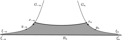
Figure 6. The ruled hexagon for measuring rate of approach of $B_{n}$ to $G_{\pm n}$

Now build polygonal loops $P_{n},\;n\in\operatorname{\mathbb{N}}$ as follows: Choose a point $\xi_{n}$ on $G_{n}$ forward of $x_{n}$ so that $d(\xi_{n},B_{n})<\delta/2$, and a point $\xi_{-n}$ on $G_{-n}$ behind $x_{-n}$ so that $d(\xi_{-n},B_{n})<\delta/2$. This is possible because $B_{n}$ is strongly asymptotic to $G_{-n}$ and $G_{n}$ in backward and forward times, and we may choose $\xi_{\pm n}$ as far away from $x_{\pm n}$ as we like. Let $\xi^{\prime}_{\pm n}$ denote the nearest points on $B_{n}$ to $\xi_{\pm n}$, respectively. Then the loop $P_{n}$ is the hexagon obtained by connecting the six points

$$x_{-n},x_{n},\xi_{n},\xi^{\prime}_{n},\xi^{\prime}_{-n},\xi_{-n}$$

in cyclic order using geodesic segments, seen in Figure 6 as the boundary of the shaded region. We can triangulate $P_{n}$ and fill it in with ruled triangles, to obtain a disk $Q_{n}$ with negatively curved interior, sides that are geodesic, and six corners at which the exterior angles (from the point of view of $Q_{n}$) are at most $\pi$. The Gaussian curvature $\kappa$ in $Q_{n}$ is negative, so the Gauss-Bonnet theorem gives us

$$\int_{Q_{n}}|\kappa|dA\leq 4\pi.$$

Now since $G_{n}$ and $G_{-n}$ are in the $\epsilon_{0}$–thick part, we were able to choose $\delta$ above so that there is an upper bound $-K_{0}<0$ for all ambient sectional curvatures at points on a $\delta$–neighborhood of $G_{\pm n}$. This gives a bound $|\kappa|\geq K_{0}$ for all points of $Q_{n}$ that are within distance $\delta$ of the edges $\overline{x_{n}\xi_{n}}$ and $\overline{x_{-n}\xi_{-n}}$.

Now if $\sigma$ is a boundary segment of $Q_{n}$ on $G_{n}$ or $G_{-n}$ of length $\lambda$ and $\sigma$ is distance more than $\delta/2$ from all of the other boundary edges, then it bounds a strip of width $\delta/2$ where $|\kappa|\geq K_{0}$, and we conclude

(6.4) $$K_{0}\lambda\delta/2\leq\int_{Q_{n}}|\kappa|dA\leq 4\pi$$

so that $\lambda\leq 8\pi/K_{0}\delta$.

Now by Lemma 6.3, for $y\in\overline{x_{n}\xi_{n}}$ we have

$$d(y,\overline{x_{n}x_{-n}})\geq ad(y,x_{n})-c$$

for $a>0$ and $c$ independent of $n$. Let $\sigma\subseteq\overline{x_{n}\xi_{n}}$ be a segment of length at least $8\pi/K_{0}\delta$ (larger than $\lambda$) starting at distance $(\delta+c)/a$ from $x_{n}$. Then every point in $\sigma$ is at least distance $\delta$ from $\overline{x_{-n}x_{n}}$. The points on $\sigma$ are also at least distance $\delta$ from $G_{-n}$, for large $n$, because $d(x_{n},x_{-n})\to\infty$ as $n\to\infty$, which implies that $d(x_{n},G_{-n})\to\infty$ using Lemma 6.3 again. The “short” sides of $P_{n}$ (the boundary of $Q_{n}$) connecting $\xi_{\pm n}$ to $\xi^{\prime}_{\pm n}$ may be assumed as far away as we like, so that they are not within distance $\delta$ of $\sigma$. Since the inequality (6.4) is violated by $Q_{n}$ as above and $n$ large enough, it follows that there is a point in $\sigma$ which is within distance $\delta/2$ of the remaining side, which lies on $B_{n}$. This is the desired point $y_{n}$ which is within distance $D:=\frac{(\delta+c)}{a}+\frac{8\pi}{K_{0}\delta}$ of $x_{n}$.

We may find $y_{-n}$ using the same argument on $G_{-n}$. ∎

6.3. Choosing $\Phi_{n}$ to control the length of $\partial Z$

Lemma 6.4.

There exist $D^{\prime},L>0$ so that for each $n$, if $\Phi_{n}$ is chosen with axis $A_{n}$ sufficiently close to $B_{n}$, then there are points $v_{n},v_{-n}\in A_{n}$ with

$$\ell_{\partial Z}(v_{\pm n})\leq L$$

and

$$d(v_{\pm n},x_{\pm n})\leq D^{\prime}$$

Proof.

Let $y_{\pm n}$ be the points obtained in Lemma 6.2. These points are within $\delta/2$ of $B_{n}$, so let us choose $\Phi_{n}$ so that $A_{n}$ is also within distance $\delta/2$ of $B_{n}$ from $\xi_{-n}$ to $\xi_{n}$ which is again possible by the Density theorem [BMM10, Theorem 6.1]. Let then $v_{\pm n}$ denote points in $A_{n}$ that are within $\delta$ of $y_{\pm n}$ respectively.

Now $\ell_{\partial Z}(x_{\pm n})=\ell_{\partial Z}(x)$ because $f_{1}$ and $f_{2}$ fix $\partial Z$. The segment from $x_{n}$ to $y_{n}$ (and $x_{-n}$ to $y_{-n}$) is of length at most $D$ and is in the $\epsilon_{0}$–thick part of Teichmüller space (by definition all $G_{\pm n}$ are in an $\epsilon_{0}$–thick part of Teichmüller space), so the lengths of all curves can change only by a bounded factor along such a segment (a thick bounded length WP segment has bounded Teichmüller length). This gives some uniform bound $L_{1}$ on $\ell_{\partial Z}(y_{\pm n})$.

Now by the convexity of the $\delta$–neighborhood of $G_{\pm n}$, the geodesic segment from $y_{\pm n}$ to $v_{\pm n}$ also stays in the $\delta$–neighborhood of $G_{\pm n}$ and hence is in the thick part of Teichmüller space, and this gives us the desired bound on $\ell_{\partial Z}(v_{\pm n})$. ∎

6.4. Choosing $\Phi_{n}$ to control ending laminations

Lemma 6.5.

There exists $A\geq 1$ so that for each $n\in\operatorname{\mathbb{N}}$, if $\Phi_{n}$ is chosen with axis $A_{n}$ sufficiently close to $B_{n}$, then there is an upper bound

$$d_{Y}(\nu^{+}(\Phi_{n}),\nu^{-}(\Phi_{n}))\leq A$$

for all $Y\subseteq S$ sharing a boundary component with $\partial Z$.

(Note the statement includes annuli $Y$ with core a component of $\partial Z$).

Proof.

First we show the bound holds for the laminations $\nu^{+}(G_{n}),\nu^{-}(G_{-n})$. Recalling the inequality (2.6) in the proof of Lemma 2.7 for any curve $\alpha$ in a Bers marking at $x$ we have that $d_{Y}(\alpha,f_{1}^{-n}(\alpha))\leq D_{\alpha}$ for all subsurfaces $Y\subseteq S$ except $X_{1}$ and annuli with core curves in $\partial X_{1}$. This implies that for an $A_{1}\geq 1$ we have

$$d_{Y}(x,x_{-n})\leq A_{1},$$

for all subsurfaces $Y$ as above. Similarly, we can see that

$$d_{Y}(x,x_{n})\leq A_{1}$$

holds for all subsurfaces $Y\subseteq S$ except $X_{2}$ and annuli with core curve in $\partial X_{2}$. Combining the above two inequalities with the triangle inequality we see that

$$d_{Y}(x_{-n},x_{n})\leq A_{2}$$

holds for all subsurfaces $Y\subseteq S$ except $X_{1},X_{2}$ and annuli with core curves in $\partial X_{1}$ and $\partial X_{2}$.

Moreover, since $G$ is the axis of a pseudo-Anosov map, $\operatorname{diam}_{\operatorname{\mathcal{C}}(Y)}(Q\circ G)$ is uniformly bounded for all $Y\subsetneq S$ (Lemma 2.7), and it follows (applying powers of $f_{2}$ or $f_{1}$) that

$$d_{Y}(x_{n},\nu^{+}(G_{n}))\leq A_{3},\qquad d_{Y}(x_{-n},\nu^{-}(G_{-n}))\leq A_{3}$$

holds for an $A_{3}\geq 1$ independent of $n$.

Putting these bounds together we find that

(6.5) $$d_{Y}(\nu^{+}(G_{n}),\nu^{-}(G_{-n}))\leq A_{4}$$

for all $Y$ except $X_{1},X_{2}$ and annuli with core curves in $\partial X_{1}$ and $\partial X_{2}$. Note that this bound holds for all $Y$ sharing a boundary curve with $Z$, since $X_{1}$ and $X_{2}$ share no boundary curves with $Z$.

Next we recall that $\nu^{+}(B_{n})=\nu^{+}(G_{n})$ and $\nu^{-}(B_{n})=\nu^{-}(G_{-n})$. Thus (6.5) holds for $(\nu^{+}(B_{n}),\nu^{-}(B_{n}))$ too.

Finally, Lemma 2.6 gives us a neighborhood $U^{+}$ of $\nu^{+}(B_{n})$ in the coarse Hausdorff topology such that, for any subsurface $Y$ sharing a boundary component with $Z$,

$$d_{Y}(\lambda,\nu^{+}(B_{n}))\leq 4$$

for any $\lambda\in U^{+}$. Similarly there is a neighborhood $U^{-}$ of $\nu^{-}(B_{n})$ with the corresponding property.

Now, the continuity theorem [BMM10, Theorem 4.7] states that, if $r$ is a recurrent ray and $r_{n}\to r$ on compact sets, then the laminations $\nu^{+}(r_{n})$ converge to $\nu^{+}(r)$ in the coarse Hausdorff topology (The theorem in [BMM10] is stated for a sequence of rays sharing a basepoint, but the proof applies in general). Thus it follows that, if $\Phi_{n}$ is chosen so that $A_{n}$ is sufficiently close to $B_{n}$, then $\nu^{+}(\Phi_{n})\in U^{+}$ and $\nu^{-}(\Phi_{n})\in U^{-}$. We thus obtain a bound of the form

$$d_{Y}(\nu^{+}(\Phi_{n}),\nu^{-}(\Phi_{n}))\leq A_{5}$$

for all $Y$ sharing a boundary component with $Z$ (this includes the annuli with core curves in $\partial Z$). This concludes the lemma. ∎

Now we may finish the

Proof of Theorem 6.1.

For each $n$, choose $\Phi_{n}$ so that the conclusions of both Lemma 6.4 and Lemma 6.5 hold.

Let $v_{n},v_{-n}$ be the points on $A_{n}$ given by Lemma 6.4. Then the segments $\overline{v_{-n}v_{n}}$ satisfy the hypotheses of Theorem 5.7: that is, the endpoints are uniformly close to $x_{-n},x_{n}$ respectively, and each of those is uniformly close to $p_{-n}$ and $q_{n}$ respectively, which are points far along the axes $g_{1}$ and $g_{2}$, where the geodesic $h$ is close to those axes. Hence $\overline{v_{-n}v_{n}}$ is a $D^{\prime\prime}$-fellow traveller of a long segment $I_{n}$ in $h$ so that $\cup_{n}I_{n}=h$, for some fixed $D^{\prime\prime}$. Moreover the length of $\partial Z$ is bounded at the endpoints $v_{\pm n}$. Thus Theorem 5.7 implies that $\inf\{\ell_{\partial Z}(x)|x\in{\overline{v_{-n}v_{n}}}\}\to 0$ as $n\to\infty$.

Lemma 6.5 gives us the inequality (6.1) for each $\Phi_{n}$. Thus the sequence $\{\Phi_{n}\}_{n}$ provides the desired pseudo-Anosov maps to complete the proof of Theorem 6.1. ∎

7. Comparison with Kleinian surface groups

In this final section we indicate how Theorems 1.4 and 1.5 can be derived from Theorem 1.3 and 6.1, respectively, using the work of Brock-Canary-Minsky on Kleinian surface groups [Min10, BCM12]. This will show that the set of short curves along a WP geodesic and the set of short curves in the corresponding hyperbolic 3-manifold do not necessarily coincide.

Recall first that a Kleinian surface group is a discrete, faithful representation $\rho:\pi_{1}(S)\to PSL(2,\operatorname{\mathbb{C}})$ which takes punctures of $S$ to parabolic elements (is type preserving). Such a representation has a pair $(\nu^{+},\nu^{-})$ of end invariant, which in particular are points of $\operatorname{Teich}(S)$ when $\rho$ is quasi-Fuchsian, and are laminations in $\operatorname{\mathcal{EL}}(S)$ when $\rho$ is doubly degenerate.

Let $N_{\rho}=\operatorname{\mathbb{H}}^{3}/\rho(\pi_{1}(S))$ be the quotient hyperbolic $3$–manifold of $\rho$. Given $\rho$ and a curve $\gamma$ in $S$ we let $\ell_{\gamma}(\rho)$ or $\ell_{\gamma}(N_{\rho})$ denote the length of the geodesic representative of $\rho$ in $N_{\rho}$. The Short Curve Theorem of [Min10] gives the following relationship between small values of $\ell_{\gamma}$ and large subsurface projections of the end invariant.

Theorem 7.1.

Suppose that $\rho:\pi_{1}(S)\to PSL(2,\operatorname{\mathbb{C}})$ is a Kleinian surface group with end invariant $(\nu^{+},\nu^{-})$ and let $N_{\rho}=\operatorname{\mathbb{H}}^{3}/\rho(\pi_{1}(S))$, then

1. for any $A\geq 1$ there is an $\epsilon>0$ so that if $\ell_{\gamma}(N_{\rho})<\epsilon$, then $\sup_{\begin{subarray}{c}Y\subsetneq S:\gamma\subseteq\partial Y\end{subarray}}d_{Y}(\nu^{+},\nu^{-})>A$.

2. for any $\epsilon>0$ there is an $A\geq 1$ so that if $\sup_{\begin{subarray}{c}Y\subsetneq S:\gamma\subseteq\partial Y\end{subarray}}d_{Y}(\nu^{+},\nu^{-})>A$, then $\ell_{\gamma}(N_{\rho})<\epsilon$.

7.1. Quasi-Fuchsian mismatch

If $p,q\in\operatorname{Teich}(S)$ we can compare the WP geodesic segment $\overline{pq}$ with the Kleinian surface group $\rho$ that $QF(p,q)=N_{\rho}$ has end invariant the pair of Bers markings at $p,q$. We recall the statement of Theorem 1.4:

Theorem 1.4. There exists $\epsilon_{1}>0$ so that for any $\epsilon>0$ there is a pair $(p,q)\in\operatorname{Teich}(S)\times\operatorname{Teich}(S)$ and a curve $\gamma$ in $S$ such that

$$\inf_{x\in\overline{pq}}\ell_{\gamma}(x)<\epsilon$$

whereas

$$\ell_{\gamma}(QF(p,q))\geq\epsilon_{1}.$$

Proof.

Given $\epsilon>0$, let $p,q$ and $\gamma$ be given by Theorem 1.3, so that

$$\inf_{x\in\overline{pq}}\ell_{\gamma}(x)<\epsilon$$

but

$$\sup\Big{\{}d_{Y}(p,q)\ |\ Y\subseteq S,\gamma\subseteq\partial Y\Big{\}}\leq A.$$

where $A$ is independent of $\epsilon$. Then part (1) of Theorem 7.1 gives an $\epsilon_{1}$ such that $\ell_{\gamma}(QF(p,q))\geq\epsilon_{1}$. ∎

7.2. Fibered mismatch

If $M_{\Phi}$ is the mapping torus of a pseudo-Anosov homeomorphism $\Phi\in\operatorname{Mod}(S)$ then $M_{\Phi}$ admits a complete hyperbolic metric by Thurston’s geometrization theorem (see e.g. [Ota01]). The manifold $M_{\Phi}$ fibers over the circle with fiber $S$, and the representation $\rho$ associated to the fiber subgroup has end invariant $(\nu^{+},\nu^{-})$ equal to the supports of the stable and unstable laminations of $\Phi$.

We are therefore led to compare the short curves of $\rho$ with those of the Weil-Petersson axis $A_{\Phi}$ of $\Phi$. We restate Theorem 1.5 here:

Theorem 1.5. There exists $\epsilon_{1}>0$ so that for any $\epsilon>0$ there is a pseudo-Anosov $\Phi\in\operatorname{Mod}(S)$ and a curve $\gamma\in S$ such that

$$\inf_{x\in A_{\Phi}}\ell_{\gamma}(x)<\epsilon$$

whereas

$$\ell_{\gamma}(M_{\Phi})>\epsilon_{1}.$$

Proof.

Given $\epsilon>0$ let $\Phi$ be the pseudo-Anosov provided by Theorem 6.1, and $\gamma$ the curve such that

$$\inf_{x\in g}\ell_{\gamma}(x)<\epsilon$$

while

$$\sup_{\begin{subarray}{c}Y\subseteq S:\gamma\subseteq\partial Y\end{subarray}}d_{Y}(\nu^{+},\nu^{-})\leq A.$$

Again by part (1) of Theorem 7.1, this produces a lower bound

$$\ell_{\gamma}(M_{\Phi})\geq\epsilon_{1}.$$

∎

References

- [BCM12] Jeffrey F. Brock, Richard D. Canary, and Yair N. Minsky, The classification of Kleinian surface groups, II: The ending lamination conjecture, Ann. of Math. (2) 176 (2012), no. 1, 1–149.
- [BH99] Martin R. Bridson and André Haefliger, Metric spaces of non-positive curvature, Grundlehren der Mathematischen Wissenschaften, vol. 319, Springer-Verlag, Berlin, 1999.
- [BKMM12] Jason Behrstock, Bruce Kleiner, Yair Minsky, and Lee Mosher, Geometry and rigidity of mapping class groups, Geom. Topol. 16 (2012), no. 2, 781–888.
- [BLMR17] Jeffrey Brock, Christopher Leininger, Babak Modami, and Kasra Rafi, Limit sets of Weil-Petersson geodesics with non-minimal ending laminations, J. Topol. Anal, to appear, arXiv:1711.01663 (2017).
- [BLMR19] by same author, Limit Sets of Weil–Petersson Geodesics, Int. Math. Res. Not. IMRN (2019), no. 24, 7604–7658.
- [BM15] Jeffrey Brock and Babak Modami, Recurrent Weil-Petersson geodesic rays with non-uniquely ergodic ending laminations, Geom. Topol. 19 (2015), no. 6, 3565–3601.
- [BMM10] Jeffrey Brock, Howard Masur, and Yair Minsky, Asymptotics of Weil-Petersson geodesics. I. Ending laminations, recurrence, and flows, Geom. Funct. Anal. 19 (2010), no. 5, 1229–1257.
- [BMM11] by same author, Asymptotics of Weil-Petersson geodesics II: bounded geometry and unbounded entropy, Geom. Funct. Anal. 21 (2011), no. 4, 820–850.
- [Bon88] Francis Bonahon, The geometry of Teichmüller space via geodesic currents, Invent. Math. 92 (1988), no. 1, 139–162.
- [Bro03] Jeffrey F. Brock, The Weil-Petersson metric and volumes of 3-dimensional hyperbolic convex cores, J. Amer. Math. Soc. 16 (2003), no. 3, 495–535.
- [Bus10] Peter Buser, Geometry and spectra of compact Riemann surfaces, Modern Birkhäuser Classics, Birkhäuser Boston Inc., Boston, MA, 2010, Reprint of the 1992 edition.
- [DW03] Georgios Daskalopoulos and Richard Wentworth, Classification of Weil-Petersson isometries, Amer. J. Math. 125 (2003), no. 4, 941–975.
- [FLP79] A. Fathi, F. Laudenbach, and V. Poenaru, Travaux de Thurston sur les surfaces, Astérisque No. 66-67 (1979), 1–286.
- [Gab09] David Gabai, Almost filling laminations and the connectivity of ending lamination space, Geom. Topol. 13 (2009), no. 2, 1017–1041.
- [Ham06] Ursula Hamenstädt, Train tracks and the Gromov boundary of the complex of curves, Spaces of Kleinian groups, London Math. Soc. Lecture Note Ser., vol. 329, Cambridge Univ. Press, Cambridge, 2006, pp. 187–207.
- [Ham15] Ursula Hamenstädt, Teichmueller flow and Weil-Petersson flow, arXiv:1505.01113 (2015).
- [KL08] Richard P. Kent, IV and Christopher J. Leininger, Shadows of mapping class groups: capturing convex cocompactness, Geom. Funct. Anal. 18 (2008), no. 4, 1270–1325.
- [Mas76] Howard Masur, Extension of the Weil-Petersson metric to the boundary of Teichmuller space, Duke Math. J. 43 (1976), no. 3, 623–635.
- [Mas92] by same author, Hausdorff dimension of the set of nonergodic foliations of a quadratic differential, Duke Math. J. 66 (1992), no. 3, 387–442.
- [Min00] Yair N. Minsky, Kleinian groups and the complex of curves, Geom. Topol. 4 (2000), 117–148 (electronic).
- [Min01] by same author, Bounded geometry for Kleinian groups, Invent. Math. 146 (2001), no. 1, 143–192.
- [Min10] Yair Minsky, The classification of Kleinian surface groups. I. Models and bounds, Ann. of Math. (2) 171 (2010), no. 1, 1–107.
- [MM99] Howard A. Masur and Yair N. Minsky, Geometry of the complex of curves. I. Hyperbolicity, Invent. Math. 138 (1999), no. 1, 103–149.
- [MM00] H. A. Masur and Y. N. Minsky, Geometry of the complex of curves. II. Hierarchical structure, Geom. Funct. Anal. 10 (2000), no. 4, 902–974.
- [Mod15] Babak Modami, Prescribing the behavior of Weil–Petersson geodesics in the moduli space of Riemann surfaces, J. Topol. Anal. 7 (2015), no. 4, 543–676.
- [Mod16] by same author, Asymptotics of a class of Weil–Petersson geodesics and divergence of Weil–Petersson geodesics, Algebr. Geom. Topol. 16 (2016), no. 1, 267–323.
- [MR18] Babak Modami and Kasra Rafi, Short curves of Teicmüller geodesics, revised, in preparation (2018).
- [Ota01] Jean-Pierre Otal, The hyperbolization theorem for fibered 3-manifolds, SMF/AMS Texts and Monographs, vol. 7, American Mathematical Society, Providence, RI; Société Mathématique de France, Paris, 2001, Translated from the 1996 French original by Leslie D. Kay.
- [Raf05] Kasra Rafi, A characterization of short curves of a Teichmüller geodesic, Geom. Topol. 9 (2005), 179–202.
- [Raf07] by same author, A combinatorial model for the Teichmüller metric, Geom. Funct. Anal. 17 (2007), no. 3, 936–959.
- [Raf14] by same author, Hyperbolicity in Teichmüller space, Geom. Topol. 18 (2014), no. 5, 3025–3053.
- [Wol87] Scott A. Wolpert, Geodesic length functions and the Nielsen problem, J. Differential Geom. 25 (1987), no. 2, 275–296.
- [Wol03] by same author, Geometry of the Weil-Petersson completion of Teichmüller space, Surveys in differential geometry, Vol. VIII (Boston, MA, 2002), Surv. Differ. Geom., VIII, Int. Press, Somerville, MA, 2003, pp. 357–393.
- [Wol08] by same author, Behavior of geodesic-length functions on Teichmüller space, J. Differential Geom. 79 (2008), no. 2, 277–334.
- [Wol10] by same author, Families of Riemann surfaces and Weil-Petersson geometry, CBMS Regional Conference Series in Mathematics, vol. 113, Published for the Conference Board of the Mathematical Sciences, Washington, DC, 2010.