Quantum Mean-Force Kinetic Theory: General Formulation and Application to Electron-Ion Transport in Warm Dense Matter

Abstract

We present an approach to extend plasma transport theory into the Warm Dense Matter (WDM) regime characterized by moderate Coulomb coupling and electron degeneracy. It is based on a recently proposed closure of the BBGKY hierarchy that expands in terms of the departure of correlations from their equilibrium value, rather than in terms of the strength of correlations. This kinetic equation contains modifications to the collision term in addition to a second term that models the non-ideal contributions to the equation of state. An explicit collision operator is derived in the semiclassical limit that is similar to that of the Uehling-Uhlenbeck equation, but where scattering is mediated by the potential of mean force (PMF). As a demonstration, we use this collision integral to evaluate temperature and momentum relaxation rates in dense plasmas. We obtain degeneracy- and coupling-dependent “Coulomb integrals” that take the place of $\ln\Lambda$ in the scattering rates. We additionally find a novel difference in the way in which degeneracy influences momentum relaxation in comparison to temperature relaxation. Finally, we evaluate electron-ion relaxation rates for the case of warm dense deuterium over a range of density and temperature spanning the classical to quantum and weak to strong coupling transitions. Results are compared with the Landau-Spitzer rate and rates obtained from the quantum Landau-Fokker-Planck equation and Lee-More model. We find that the models diverge significantly in the degenerate and moderately coupled regime and attribute this difference to how the various models treat the physics of Pauli blocking, correlations, large-angle scattering, and diffraction.

I Introduction

Physical models are often based on expansions in small parameters about some more simple state. For instance in plasma physics transport properties are traditionally calculated from an expansion in which the ratio of the average potential energy to kinetic energy (the Coulomb coupling parameter $\Gamma=\left\langle U\right\rangle/\left\langle K\right\rangle$) is taken to be small. In Fermi liquid theory, the coupling may be strong, but the ratio of the temperature to the Fermi energy (the inverse degeneracy parameter $\Theta=T/E_{F}$) is taken to be small. In solid state physics, a rigid or semi-rigid ion lattice provides a zero-order structure about which to base a perturbation expansion. Warm Dense Matter (WDM) is defined by the condition that neither the deviation from an ideal plasma, nor from a zero-temperature Fermi liquid, nor from a rigid lattice structure, can be taken to be small. This occurs in experiments involving extreme compression of materials (Glenzer et al., 2016; Riley, 2018; Mančić, 2010), in astrophysics (Redmer et al., 2008; Koenig et al., 2005), and along the compression path in inertial confinement fusion (ICF) experiments (Hu et al., 2015). As a result of the demanding conditions for theoretical modeling, the description of WDM has been highly reliant on computational techniques. However, ab initio computation proves too expensive for many problems in WDM, whereas faster methods often involve uncontrolled approximations or have uncertain applicability in WDM conditions. In order to support computational efforts, explore larger regions of parameter space, and expediently provide data tables for hydrodynamic simulations, reliable and fast tools for the computation of transport coefficients in dense plasmas and WDM remain desirable.

In this work, we apply a new expansion parameter to quantum kinetic theory to develop a model for transport in plasmas subject to electron degeneracy and Coulomb coupling - thus providing an expansion parameter suitable for WDM. The model is derived via an extension of a novel closure (Baalrud and Daligault, 2019) of the BBGKY hierarchy to the quantum domain. Rather than expanding about small density or weak coupling, the new closure expands in terms of the departure of correlations from their equilibrium values. In the classical case this model shows that two particles in the plasma interact via the potential of mean force, and it has proven successful at predicting ion transport in both classical and dense plasmas with moderate coupling (Baalrud and Daligault, 2013, 2014; Daligault et al., 2016). Here, we develop the extension of this theory into the quantum domain to derive quantum mean force kinetic theory (QMFKT). The modified BBGKY hierarchy can be closed at any level, which leads to a formal integrodifferential equation for the reduced Wigner distributions. The “free-streaming” part of the equation in our case contains a new term associated with the excess pressure; i.e., the model incorporates non-ideal effects in the equation of state. Meanwhile, the new collision term contains the effects of correlations, approximated by their equilibrium limit. Further reduction of the BBGKY hierarchy to a Boltzmann-type equation is complicated by coupled momentum and position dependence of the reduced Wigner functions due to the uncertainty principle. To obtain an immediately useful transport equation without neglecting diffraction or Pauli blocking, we apply a semi-classical approximation. The smallness of the electron-ion mass ratio justifies the application of this approach to electron-ion collisions in plasmas in which the electron coupling and degeneracy are small to moderate. By closing the resulting hierarchy at second order, and applying the molecular chaos approximation, we obtain a convergent quantum collision operator that is in the form of the Boltzmann-Uehling-Uhlenbeck (BUU) equation, except where the particles scatter via the potential of mean force rather than the Coulomb potential. The model in this limit is particularly suitable for the description of electron-ion relaxation processes in WDM conditions, and as a demonstration we apply it to the calculation of relaxation rates in warm dense deuterium.

The approximate regimes in which these different physical processes are important can be roughly understood in terms of the degeneracy parameter $\Theta$ and Coulomb coupling parameter $\Gamma$. Because of degeneracy, the electron Coulomb coupling can differ from that of the ions even at the same temperature with single ionization. This is due to the average speed of electrons shifting from the thermal speed to the Fermi speed as degeneracy increases, a phenomenon that causes electrons to become increasingly weakly coupled at high density. This can be seen through the definition $\Gamma=\left\langle U\right\rangle/\left\langle K\right\rangle$ with the statistical averages taken using a Maxwell-Boltzmann distribution for ions and a Fermi-Dirac distribution for electrons so that

$$\Gamma_{i}=\frac{Z^{2}e^{2}/a}{k_{B}T},$$ (1)

and

$$\Gamma_{e}=\Gamma_{i}\frac{{\rm Li}_{3/2}\left[-\exp(\mu/k_{{\rm B}}T)\right]}{{\rm Li}_{5/2}\left[-\exp(\mu/k_{{\rm B}}T)\right]},$$ (2)

where $a=(3/4\pi n)^{1/3}$ is the Wigner-Seitz radius, ${\rm{\rm Li}}$ is the polylogarithm function (closely related to the Fermi integral) and $\mu$ is the electron chemical potential related to $\Theta$ through the normalization of the Fermi-Dirac distribution (Melrose and Mushtaq, 2010):

$$-{\rm Li}_{3/2}\left[-\exp(\mu/k_{{\rm B}}T)\right]=\frac{4}{3\sqrt{\pi}}\Theta^{-3/2}.$$ (3)

The conditions $\Gamma=1$ and $\Theta=1$ divide the density-temperature parameter space into multiple regions, as seen in figure 1. The regimes can be broken down into (a) classical weak coupling, (b) classical strong coupling, (c) quantum weak coupling, and (d) classical strongly coupled ions with degenerate weak or strongly coupled electrons. WDM exists at the intersection of all of these regions marked by the blue region, where no small expansion parameter has been available. Transport in region (a) is well-understood in terms of the Landau-Spitzer theory, and region (c) has been successfully modeled through quantum weak-coupling theories such as the quantum Landau-Fokker-Planck equation (Daligault, 2016). Progress has recently been made extending classical plasma transport theory into region (b) for $\Gamma\lesssim 20$ through use of mean force kinetic theory (MFKT) (Baalrud and Daligault, 2013, 2014, 2019), which has also been successfully applied in region (d) for WDM in the case of ion transport (Daligault et al., 2016). Here, we broaden this approach to include electron degeneracy in the dynamics.

Existing theoretical methods for predicting transport in WDM typically fall into the categories of binary collision theories (Daligault, 2016, 2018; Gericke et al., 2002; Lee and More, 1984; Starrett, 2018), linear response theories (Daligault and Dimonte, 2009; Lampe, 1968; Scullard et al., 2018), and non-equilibrium Green’s functions and field-theoretic methods (Brown et al., 2005; Brown and Singleton, 2007; Singleton, 2007; Balzer and Bonitz, 2013; Bonitz, 2016). In this work we overcome some limits of existing methods by performing a controlled expansion, and in the quasi-classical limit the resulting model is physically intuitive and can be evaluated relatively quickly. The model in this limit is expected to be valid for plasmas with weak and moderate coupling ($\Gamma\lesssim 20$) and classical or moderately degenerate electrons, when $m_{e}T_{i}\ll m_{i}T_{e}$, and when the system correlations are well-approximated by their equilibrium limit. The extension of this region beyond the currently well-described regions is shown as the green area in figure 1. For the case of warm dense deuterium, we evaluate the model and some common and simple alternatives and discuss the relative importance of the effects of correlation, large-angle scattering, Pauli blocking, and diffraction. We use this scheme to select three densities at which to evaluate the model for warm dense deuterium in order to access regimes with a different physical process dominating in each.

We begin by deriving our kinetic theory from the quantum Liouville equation in section II. We introduce the new closure and, in the limit that electron coupling and degeneracy are small to moderate, obtain a quasi-classical potential of mean force that moderates two-body interactions in the plasma. From there we obtain a quantum kinetic equation, in which the collision operator is similar to the BUU collision operator, but where correlation effects arise in the scattering cross section via the potential of mean force. In section IV we apply this to electron-ion momentum and temperature relaxation, where we obtain degeneracy- and correlation-dependent “Coulomb integrals” that replace the traditional Coulomb logarithm. We compare the relaxation rates predicted from our theory with other common models in an experimentally relevant parameter regime in section V. We conclude and summarize in section VI.

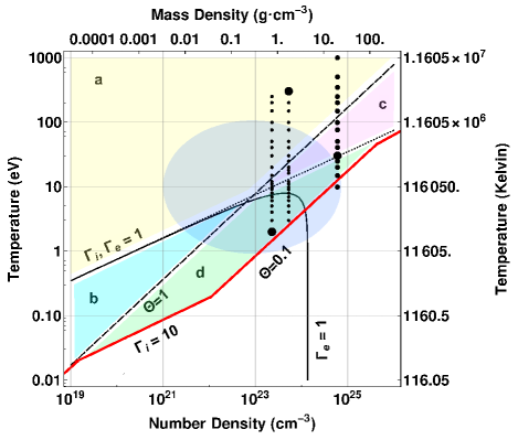
Figure 1: Parameter regimes of plasmas. The solid black line is the boundary between weak and strong electron coupling $\Gamma_{e}=1$ and turns over due to the electron degeneracy; the dotted lined is the separation between weak and strong ion coupling $\Gamma_{i}=1$; and the dashed line is the separation between classical and degenerate electrons $\Theta=1$. The darker blue oval denotes the sector of Warm Dense Matter. Region a (yellow) is classical weakly coupled plasma; region b (light blue) is characterized by classical strong coupling; region c (pink) by quantum weak coupling, and region d (green) by both quantum electrons and strongly-coupled ions. We expect QMFKT to apply to each region a-d. The red line demarcates the region of validity of plasma-type transport theories; beyond this is the regime of condensed matter. Dots are points at which the theory is evaluated, with the bold dots being presented in figure 6.

II Quantum Mean Force Kinetic Theory

Quantum kinetic theory has been developed partly in parallel with the historical development of plasma kinetic theory and partly as a result of the demands of advances in solid state physics and high energy density physics. An overview of the subject can be found in (Bonitz, 2016). Beginning with the quantum Liouville equation for the Wigner quasi-probability distribution, we will now develop a closure scheme for the quantum BBGKY hierarchy in which the new closure parameter quantifies the departure of the correlations in the system from their equilibrium values.

II.1 Wigner Functions and the Quantum BBGKY Hierarchy

Our theory is developed in terms of the many-body Wigner function $f^{(N)}$, which contains equivalent information to the $N-{\rm body}$ wavefunction, i.e. it completely specifies the state of the system. The Wigner function evolves according to the quantum Liouville equation (Imam-Rahajoe and Curtiss, 1967; Hoffman et al., 1965)

$$\frac{\partial f^{(N)}\left(1,2...N;t\right)}{\partial t}+\sum_{i=1}^{N}\frac{\boldsymbol{p}_{i}}{m_{i}}\cdot\nabla_{i}f^{(N)}\left(1,2...N;t\right)$$

$$+\text{$\mathscr{O}$}\cdot f^{(N)}\left(1,2...N;t\right)=0$$

with a local potential $U(\boldsymbol{r}_{N})$ which is a function of the $3N$ coordinates $\boldsymbol{r}_{N}$ of the $N$ particles. Here the notation $\left(1,2...N\right)$ means the set of all $N$ positions and momenta $\left(\{\boldsymbol{\boldsymbol{r}}_{N}\},\left\{\boldsymbol{p}_{N}\right\}\right)$ and

$$\text{$\mathscr{O}$}\cdot f^{(N)}=-\frac{2}{\hbar}\sin\left[\frac{\hbar}{2}\frac{\partial^{U}}{\partial\boldsymbol{r}_{N}}\cdot\frac{\partial^{f}}{\partial\boldsymbol{p}_{N}}\right]U(\boldsymbol{r}_{N})f^{(N)}(1,2...N;t),$$ (4)

in which the superscripts $U$ and $f$ refer to the function on which the derivatives operate. The derivatives represent $3N-{\rm dimensional}$ gradients, and the $\sin$ operator is defined via its power series. For a pairwise (e.g. Coulomb) potential $\phi(\boldsymbol{r}_{ij})$ with no external fields,

$$U(\boldsymbol{r}_{N})=\frac{1}{2}\sum_{i=1}^{N}\sum_{j=1,\thinspace j\neq i}^{N}\phi_{ij}(\boldsymbol{r}_{i},\boldsymbol{r}_{j}),$$ (5)

and

$$\text{$\mathscr{O}$}=-\frac{1}{\hbar}\sum_{i=1}^{N}\sum_{j=1,\thinspace j\neq i}^{N}\sin\left[\frac{\hbar}{2}\frac{\partial^{\phi}}{\partial\boldsymbol{r}_{ij}}\cdot\frac{\partial}{\partial\boldsymbol{p}_{i}}\right]\phi(\boldsymbol{r}_{ij}),$$ (6)

where $\boldsymbol{r}_{ij}=\boldsymbol{r}_{i}-\boldsymbol{r}_{j}$. To facilitate comparison with the Liouville equation, we expand the $\sin$ operator,

$$\left\{\frac{\partial}{\partial t}+\sum_{i=1}^{N}\left[\frac{\boldsymbol{p}_{i}}{m_{i}}\cdot\frac{\partial}{\partial\boldsymbol{r}_{i}}-\frac{1}{\hbar}\sum_{j=1,\thinspace j\neq i}^{N}\sum_{k=0}^{\infty}\frac{(-1)^{k}}{(2k+1)!}\left(\frac{\hbar}{2}\right)^{2k+1}\frac{\partial^{2k+1}\phi(\boldsymbol{r}_{ij})}{\partial\boldsymbol{r}_{ij}^{k+1}}\cdot\frac{\partial}{\partial\boldsymbol{p}_{i}^{2k+1}}\right]\right\}f^{(N)}\left(1,2...N;t\right)=0\;.$$ (7)

The classical Liouville equation is obtained by keeping only the first term of the sum over $k$. To maintain similarity with the classical case, we write the quantum Liouville equation as

$$\left\{\frac{\partial}{\partial t}+\sum_{i=1}^{N}\left[L_{i}+\sum_{j=1,\thinspace j\neq i}^{N}L_{ij}^{QC}\right]\right\}f^{(N)}\left(1,2...N;t\right)=0,$$ (8)

where

$$L_{i}\equiv\frac{\boldsymbol{p}_{i}}{m_{i}}\cdot\frac{\partial}{\partial\boldsymbol{r}_{i}},$$ (9)

and

$$L_{ij}^{QC}\equiv-\frac{1}{\hbar}\sum_{k=0}^{\infty}\frac{(-1)^{k}}{(2k+1)!}\left(\frac{\hbar}{2}\right)^{2k+1}\frac{\partial^{2k+1}\phi(\boldsymbol{r}_{ij})}{\partial\boldsymbol{r}_{ij}^{2k+1}}\cdot\frac{\partial}{\partial\boldsymbol{p}_{i}^{2k+1}},$$ (10)

is the “quantum Coulomb” operator. Equations (8)-(10) are an exact description of the $N-{\rm body}$ problem.

As is true classically, full knowledge of the N-body problem is not necessary to specify the important parameters of the system. Instead, the $n{\rm{}^{\prime}th}$ reduced Wigner function, obtained by integrating the N-body Wigner function over some fraction $N-n$ of the particle phase space

$$f^{(n)}(1,2...,N;t)\equiv\frac{N!}{(N-n)!}\int d\boldsymbol{r}^{(N-n)}d\boldsymbol{p}^{(N-n)}f^{(N)},$$ (11)

where $d\boldsymbol{x}^{n}=d\boldsymbol{x}_{1}d\boldsymbol{x}_{2}\ldots d\boldsymbol{x}_{n}$, is sufficient to calculate observables that depend on $n$ or fewer particle coordinates. For example, the fluid variables number density, drift velocity, pressure, and energy-density can be determined from the reduced one-particle Wigner functions.

If the quantum Liouville equation is integrated over the $N-n$ subspace coordinates, an equation of motion for the $n-{\rm body}$ reduced Wigner function $f^{(n)}\left(1,2...n;t\right)$ is obtained. Averaging over the positions and momenta of particles $n$, $n+1$… $N$, utilizing the symmetry of the Wigner function under exchange of particle indices, provides the quantum BBGKY hierarchy

$$\left[\frac{\partial}{\partial t}+\sum_{i=1}^{n}\left(L_{i}+\sum_{j=1,\thinspace j\neq i}^{N}L_{ij}^{QC}\right)\right]f^{(n)}(1,2,...n;t)$$

$$=-\sum_{i=1}^{n}\int\int d^{3}r_{n+1}d^{3}p_{n+1}L_{i,n+1}^{QC}f^{(n+1)}(1,2,...n+1;t).$$ (12)

An approximation is needed in order to close the hierarchy and make calculations using only the first $n$ reduced functions. Typically, the approximation that is made involves the assumption that $f^{(n+1)}=0$, implying weak correlations, in order to neglect dependence on the $n+1$ and higher-order distributions. In the following, we will follow a recent approach that has been applied to the classical limit (Baalrud and Daligault, 2019) and instead make the approximation that the system is close to equilibrium, without neglecting correlations.

II.2 Expansion Parameter and Closure Approximation

Typically, equation (12) is closed at a given level $n$ by making some assumption about the unimportance of correlations at the level $n+1$, thus simplifying or neglecting the $f^{(n+1)}$ dependence on the right-hand side (RHS). However, this approximation neglects correlations and is not justified in even a weakly-coupled plasma because screening is important. To obtain a convergent kinetic equation, we instead re-write the equation in terms of a new expansion parameter that does not explicitly depend on the strength of the interaction or the density. We define the relative deviation of the $n+1{\rm-body}$ Wigner function from equilibrium as

$$\frac{\Delta f^{(n+1)}}{f_{0}^{(n+1)}}\equiv\frac{f^{(n+1)}}{f_{0}^{(n+1)}}-\frac{f^{(n)}}{f_{0}^{(n)}}.$$ (13)

Adding and subtracting the second term on the right hand side of this definition to the BBGKY equation and rearranging, we express $\Delta f$ as the expansion parameter:

$$\Bigg{\{}\frac{\partial}{\partial t}+\sum_{i=1}^{n}\Bigg{[}L_{i}+\sum_{j=1,\thinspace j\neq i}^{n}L_{ij}^{QC}$$

$$+\int\int d^{3}r_{n+1}d^{3}p_{n+1}L_{i,n+1}^{QC}\frac{f_{0}^{(n+1)}}{f_{0}^{(n)}}\Bigg{]}\Bigg{\}}f^{(n)}$$ (14)

$$=-\sum_{i=1}^{n}\int\int d^{3}r_{n+1}d^{3}p_{n+1}L_{i,n+1}^{QC}\Delta f^{(n+1)}.$$ (15)

The operator $L_{i,n+1}^{QC}$ in the last term on the LHS is understood to contain derivatives that operate on both the equilibrium Wigner functions and the $f^{(n)}$ term. Like the original BBGKY equation, this is an exact description of the plasma. However, the RHS is now proportional to a quantity which is by definition small for a system near equilibrium. Closure can then be obtained naturally at any level $n$ of the hierarchy by taking $\Delta f^{(n+1)}=0$. The remainder on the LHS and the first $n-1$ equations then describe the effective dynamics of $n$ particles in the presence of the static influence of particles $n+1\ldots N$ within the equilibrium reduced Wigner function $f_{0}^{(n+1)}$ on the LHS.

The relevant operator is the new term on the left hand side

$$\sum_{i=1}^{n}\int\int d^{3}r_{n+1}d^{3}p_{n+1}L_{i,n+1}^{QC}\left(\frac{f_{0}^{(n+1)}}{f_{0}^{(n)}}\right).$$ (16)

In the classical case this term can be shown to combine with the free-particle operator $L_{i}$ to become a new two-body interaction operator containing the potential of mean force (Baalrud and Daligault, 2019). However, the equilibrium Wigner functions differ from the classical distributions in that they must encapsulate the uncertainty and Pauli-exclusion principles. Specifically, the $f_{0}^{(n)}$ do not decouple into independent functions of the positions and momenta of the particles due to the uncertainty principle. In the classical limit, the ratio $f_{0}^{(n+1)}/f_{0}^{(n)}$ depends on the momentum $\boldsymbol{p}_{n+1}$ only through a factor $\exp\boldsymbol{p}_{n+1}$, and after the integration over $\boldsymbol{p}_{n+1}$ the momentum derivative in the $L_{i,n+1}$ operator therefore commutes through this ratio. Without this simplification, it is not clear how to write a new operator in the form $\nabla W_{ij}\cdot\partial f^{(n)}/\partial p_{ij}$, and therefore unclear how to explicitly obtain a potential of mean force. Furthermore, the $1-{\rm particle}$ momentum distribution for a fermion does not have simple Maxwellian dependence but instead is a Fermi-Dirac distribution. This complicates the derivation, and the former even obscures the meaning of the potential of mean force for a general quantum system due to the dependence on momentum.

Nevertheless, the closed hierarchy represents a formal approximate solution. Kinetic theories provide closed equations for the single-particle distribution. This may be obtained through closure at the second hierarchy equation. Taking $\Delta f^{(3)}=0$, the system is described by the first level equation

$$\left[\frac{\partial}{\partial t}+L_{1}+\int\int d^{3}r_{2}d^{3}p_{2}L_{12}^{QC}\frac{f_{0}^{(2)}\left(1,2\right)}{f_{0}^{(1)}\left(1\right)}\right]f^{(1)}$$ (17)

$$=-\int\int d^{3}r_{2}d^{3}p_{2}L_{12}^{QC}\Delta f^{(2)}$$ (18)

and the second level equation

$$\Bigg{\{}\frac{\partial}{\partial t}+L_{1}+L_{2}+L_{12}^{QC}+L_{21}^{QC}$$

$$+\int\int d^{3}r_{3}d^{3}p_{3}\left[\left(L_{13}^{QC}+L_{23}^{QC}\right)\frac{f_{0}^{(3)}}{f_{0}^{(2)}}\right]\Bigg{\}}f^{(2)}=0.$$ (19)

Consider the first level equation; typically, the LHS would describe the free streaming motion of a particle while the RHS encapsulates its interaction with the rest of the plasma, i.e. the collision operator. In this new scheme however, the last term on the LHS depends on the equilibrium correlations of the rest of the plasma. This term is associated with the non-ideality of the plasma. Taking the momentum moment $\int d\boldsymbol{p}_{1}\boldsymbol{p}_{1}\left\{\cdots\right\}$, the gradient of the ideal pressure results from the free-streaming term $\int d\boldsymbol{p}_{1}\boldsymbol{p}_{1}L_{1}f^{(1)}=\nabla P_{k}$ where $nk_{B}T$ is the ideal component of the pressure while the new term is

$$\int d\boldsymbol{p}_{1}\boldsymbol{p}_{1}\int\int d\boldsymbol{r}_{2}d\boldsymbol{p}_{2}L_{12}^{QC}\frac{f_{0}^{(2)}\left(1,2\right)}{f_{0}^{(1)}\left(1\right)}.$$ (20)

In the limit of a Maxwellian distribution and $\hbar\rightarrow 0$, it has been shown (Baalrud and Daligault, 2019) that this becomes exactly the gradient of the excess pressure $p_{\phi}=-(\rho^{2}/6)\int_{0}^{\infty}dr\phi^{\prime}(r)rg(r)$ in classical mechanics (Hansen and McDonald, 2006), where $r=|\boldsymbol{r}_{1}-\boldsymbol{r}_{2}|$. Whether such an analytic reduction exists in the quantum case remains to be seen, but it seems clear that the interpretation can be carried over.

Considering the second equation of the hierarchy (19), this can be seen as an integrodifferential equation for the reduced Wigner function $f^{(2)}$. Knowledge of $f^{(2)}$ and thus $\Delta f^{(2)}$ would provide the collision operator that would appear on the RHS of equation (17). A direct solution of equation (19) would allow direct calculation of transport coefficients for plasmas of arbitrary constituency, strong degeneracy and with weak to moderate coupling. However, such a general solution seems unlikely except under conditions in which the operator (16) simplifies. We will for now restrict ourselves to a semiclassical limit that fulfills these conditions.

III Semi-classical Limit

In order to make further progress, and as a demonstration of the theory, in addition to the closure approximation $\Delta f^{(3)}\ll f_{0}^{(3)}$ we from this point onward assume a limit in which the operator (16) is well-approximated by its classical limit. We will proceed to justify this specifically for the case of electron-ion interactions in the limit that the ions are classical and the electron degeneracy and coupling are both moderate, but it is also applicable to ion-ion collisions and semiclassical electron-electron collisions. This can be seen through application of the semi-classical Wigner-Kirkwood expansion in $\hbar$ for the functions $f_{0}$. The expressions are lengthy and the details have been reserved for Appendix A. Applying the results of Shalitin (Shalitin, 1973), we can write e.g.

$$\frac{f_{0}^{(n+1)}}{f_{0}^{(n)}}\approx\left(\frac{m}{2\pi k_{B}T}\right)\exp\left(-\frac{1}{2mk_{B}T}p_{n+1}^{2}\right)$$ (21)

$$\times\frac{\rho_{n+1}(\boldsymbol{r}_{1},...,\boldsymbol{r}_{n+1})}{\rho_{n}(\boldsymbol{r}_{1},...,\boldsymbol{r}_{n})}\left[1+\left(\frac{Q_{n+1}}{C_{n+1}}-\frac{Q_{n}}{C_{n}}\right)\right]$$ (22)

where

$$\rho_{n}\equiv\frac{N!}{(N-1)!}\frac{\int d\boldsymbol{r}^{(N-n)}\exp\left[-V_{N}/k_{B}T\right]}{\int d\boldsymbol{r}^{(N)}\exp\left(-V_{N}/k_{B}T\right)}$$ (23)

is the $n-{\rm body}$ correlation function with $V_{N}\equiv\sum_{i=1}^{N}\sum_{j>i}^{N}\phi_{ij}$ being the total electrostatic potential energy and where the $Q$ and $C$ functions are integrals of combinations of gradients of the potential and contain the sole dependence on the momenta of particles $1$ through $n$; see Appendix A. Furthermore, these terms are of second and higher order in the potential, and are second order in terms of quantum effects. They are thus suppressed by the classical nature of the ions and lack of strong coupling of the electrons, a condition that is well-matched in the WDM regime. We therefore approximate $f_{0}^{(n)}=\rho_{n}(\boldsymbol{r}^{(n)})\Pi_{i}^{n}f_{M}^{(1)}(\boldsymbol{p}_{i})$ so that

$$\frac{f_{0}^{(n+1)}}{f_{0}^{(n)}}\approx\frac{\rho_{n+1}(\boldsymbol{r}_{1},...,\boldsymbol{r}_{n+1})}{\rho_{n}(\boldsymbol{r}_{1},...,\boldsymbol{r}_{n})}f_{M}^{(1)}\left(\boldsymbol{p}_{n+1}\right),$$ (24)

where $f_{M}$ is the Maxwellian distribution. This separation of the position and momentum dependence results in a momentum-independent potential of mean force, but necessitates restriction of the current theory to the semiclassical limit. Without this assumption it is unclear how to interpret the last term on the LHS of equation (15). With this approximation, we obtain

$$\frac{1}{\hbar}\sum_{k=0}^{\infty}\left(\frac{\hbar}{2}\right)^{2k+1}\frac{(-1)^{k}}{(2k+1)!}\Bigg{\{}\sum_{j=1,\thinspace j\neq i}^{n}\frac{\partial^{k}\phi}{\partial\boldsymbol{r}_{ij}^{k}}-$$ (25)

$$\int d\boldsymbol{p}_{n+1}f_{M}^{(1)}(\boldsymbol{p}_{n+1})\int d\boldsymbol{r}_{n+1}\frac{\rho_{n+1}}{\rho_{n}}\frac{\partial^{2k+1}\phi}{\partial\boldsymbol{r}_{i,n+1}^{2k+1}}\Bigg{\}}$$ (26)

$$=-\sum_{j=1,\thinspace j\neq i}^{n}\frac{1}{\hbar}\sum_{k=0}^{\infty}\frac{(-1)^{k}}{(2k+1)!}\left(\frac{\hbar}{2}\right)^{2k+1}\frac{\partial^{2k+1}W^{(n)}}{\partial\boldsymbol{r}_{i}^{2k+1}}$$ (27)

where

$$\frac{\partial^{2k+1}W^{(n)}}{\partial\boldsymbol{r}_{i}^{2k+1}}\equiv\sum_{j=1,\thinspace j\neq i}^{n}\frac{\partial^{2k+1}\phi}{\partial\boldsymbol{r}_{ij}^{2k+1}}$$

$$+\int d\boldsymbol{p}_{n+1}f_{M}^{(1)}(\boldsymbol{p}_{n+1})\int d\boldsymbol{r}_{n+1}\frac{\rho_{n+1}}{\rho_{n}}\frac{\partial^{2k+1}\phi}{\partial\boldsymbol{r}_{i,n+1}^{2k+1}}$$ (28)

defines what can properly be interpreted as the potential of mean force $W^{(n)}$. The BBGKY hierarchy can be re-written with the mean-force potential absorbing the $f_{0}$ terms on the LHS and the Coulomb-force term

$$\left\{\frac{\partial}{\partial_{t}}+\sum_{i=1}^{n}\left[L_{i}+\bar{L}_{i}^{Q}\right]\right\}f^{(n)}=$$

$$-\sum_{i=1}^{n}\int\int d\boldsymbol{r}_{n+1}d\boldsymbol{p}_{n+1}L_{i,n+1}^{QC}\Delta f^{(n+1)}\left(1,2...n+1\right)$$

where

$$\bar{L}_{i}^{Q}\equiv-\frac{1}{\hbar}\sum_{k=0}^{\infty}\frac{(-1)^{k}}{(2k+1)!}\left(\frac{\hbar}{2}\right)^{2k+1}\frac{\partial^{2k+1}W^{(n)}}{\partial\boldsymbol{r}_{i}^{2k+1}}\cdot\frac{\partial}{\partial\boldsymbol{p}_{i}^{2k+1}}$$ (29)

now describes $n-{\rm body}$ interactions through the potential of mean force $W^{(n)}$. This takes the same form as the initial hierarchy equation, but the force operator on the LHS has been modified and now depends on the equilibrium Wigner functions at the $n+1$ level. Finally, we note that this semiclassical limit of the potential of mean force can be written in terms of the correlation function

$$g^{(n)}(\boldsymbol{r}_{1},...,\boldsymbol{r_{n}})\equiv\rho^{(n)}(\boldsymbol{r}_{1},...,\boldsymbol{r_{n}})/\Pi_{i=1}^{n}\rho^{(1)}(\boldsymbol{r}_{i})$$ (30)

as

$$W^{(n)}=-k_{B}T\ln g^{(n)},$$ (31)

which provides direct connection between the potential of mean force and the structural properties of the plasma.

III.1 Derivation of a Boltzmann-Uehling-Uhlenbeck-like Equation

The theory at this point is written in the form of the original BBGKY equation, but with the Coulomb interaction operator $L_{ij}^{QC}$ being replaced by the mean-force operator $\bar{L}_{i}^{Q}$. Classically, the Boltzmann equation is derived by closing at the second level of the hierarchy. With the new operator $\bar{L}_{i}^{Q}$, equations (17-19) become

$$\left[\frac{\partial}{\partial t}+L_{1}+\int\int d\boldsymbol{r}_{2}d\boldsymbol{p}_{2}L_{12}^{QC}\frac{\rho_{2}\left(|r_{1}-r_{2}|\right)}{\rho_{1}\left(r_{1}\right)}f_{M}\left(\boldsymbol{p}_{2}\right)\right]f^{(1)}$$

$$=-\int\int d\boldsymbol{r}_{2}d\boldsymbol{p}_{2}L_{12}^{QC}\Delta f^{(2)}$$ (32)

$$\left(\frac{\partial}{\partial t}+L_{1}+L_{2}+\bar{L}_{1}^{Q}+\bar{L}_{2}^{Q}\right)f^{(2)}=0,$$ (33)

where now the closed $n=2$ equation describes the evolution of two particles under the influence of the potential of mean force. Classically the Boltzmann equation can be obtained here by taking the so-called Boltzmann-Grad limit (Grad, 1958), with the associated approximation of molecular chaos (scattering particle initially uncorrelated), this procedure remains unmodified in the classical MFKT (Baalrud and Daligault, 2019). The derivation of the BUU equation rests on more uncertain ground. Originally proposed by Uehling and Uhlenbeck (Uehling and Uhlenbeck, 1933), a more rigorous definition was attempted in terms of the Wigner function in references (Imam-Rahajoe and Curtiss, 1967; Hoffman et al., 1965; Ross and Kirkwood, 1954). However, the situation remains unsettled, with the most rigorous derivations of the BUU equation being obtained in the density-matrix formalism by Snider (Snider et al., 1995) and Boercker and Duffty (Boercker and Dufty, 1979). The result ultimately is indeed the BUU equation written in terms of a scattering T-matrix that plays an analogous role to the differential cross section. There is a caveat: the scattering problem must be solved with the intermediate states of any perturbation expansion respecting exchange symmetry. We argue that in our formalism this is accounted for within the potential itself: the mean-force potential contains the statistical information regarding spectator particles that “dress” the interaction. We further argue that steps in the past derivations of the BUU equation are not affected negatively by the presence of the mean-force potential, and can be carried over to our case. The closure approximation and the molecular chaos assumption still restrict the range of validity of the theory by limiting the extent to which correlations are included, which restricts the theory to moderate values of $\Gamma$, as is also true in the classical case (Baalrud and Daligault, 2019).

The resulting collision integral is that of Uehling and Uhlenbeck

$$C_{q}^{ss^{\prime}}=\int d\boldsymbol{v}^{\prime}d\Omega\frac{d\sigma}{d\Omega}u\left[\hat{f_{s}}\hat{f_{s^{\prime}}}\left(1+\theta_{s}f_{s}\right)\left(1+\theta_{s^{\prime}}f_{s^{\prime}}\right)-f_{s}f_{s^{\prime}}\left(1+\theta_{s}\hat{f_{s}}\right)\left(1+\theta_{s}\hat{f_{s^{\prime}}}\right)\right],$$ (34)

where the “hatted” quantities $\hat{f_{s}}$ are evaluated at the post-collision velocity $\hat{\boldsymbol{v}}=\boldsymbol{v}+\Delta\boldsymbol{v}$ and $\theta_{s}=(\pm 1/g_{s})(h/m_{s})^{3}$ where $g_{s}$ is an integer accounting for particle statistics, the $+$ sign corresponds with bosons and the $-$ sign with fermions. The difference between this and the established BUU collision operator is that in the calculation of the differential cross section $d\sigma/d\Omega$ the scattering potential is now the potential of mean force. This can be obtained through solution of the radial Schrödinger equation

$$\left\{\frac{d^{2}}{dr^{2}}+\left[k^{2}-\frac{l(l+1)}{r^{2}}-\frac{2m}{\hbar^{2}}W_{ss^{\prime}}^{(2)}(r)\right]\right\}R_{l}=0$$ (35)

via a partial wave expansion, where $W_{ss^{\prime}}^{(2)}=-k_{B}T\ln g_{ss^{\prime}}(|r_{1}-r_{2}|)$ is the $n=2$ limit of equation (31) in terms of the pair correlation function $g_{ss^{\prime}}(|r_{1}-r_{2}|)\equiv g_{ss^{\prime}}^{(2)}(\boldsymbol{r}_{1},\boldsymbol{r}_{2})$. Calculation of the differential cross section can be performed through standard quantum scattering theory (Landau and Lifshitz, 1965).

Here we summarize the approximations that have been made to obtain this collision integral. First, we made the closure approximation $\Delta f^{(3)}/f_{0}^{(3)}\ll 1$, meaning that the triplet distribution function of a given species is close to its equilibrium limit. Furthermore, we made the quasi-classical assumption that the product of the degeneracy and coupling parameters was not overly large. For electron-ion interactions, this can be justified by the smallness of the electron-ion mass ratio. Finally, we assume Markovian collisions and molecular chaos, the latter of which again is justified for the case of electron-ion collisions (whereas for electron-electron collisions one cannot assume $f^{(2)}(1,2)=f^{(1)}(1)f^{(1)}(2)$ without violating exchange symmetry). These approximations make for a model that is well-suited for the electron-ion collisions in the WDM regime.

III.2 The Potential of Mean Force

The interpretation of this result is that particles in a strongly coupled plasma do not collide in isolation. Instead of fully treating the dynamics of an $n>2$ body collision, the theory shows that the dynamics are approximated by an effective 2-body interaction obtained by canonically averaging over the phase-space of the remaining $N-2$ particles at equilibrium. This is similar to the reasoning that leads to the use of screening potentials of the Yukawa type, and indeed the mean-force theory reduces to a Debye screened binary collision theory in the weakly-coupled classical limit. However, the classical Debye-Huckel, or quantum Thomas-Fermi, potentials do not account for correlation effects. Correlations are included in our theory through the presence of the correlation function $\rho_{n}$ in equation (28). Specifically, for $2-$body collisions in a uniform plasma, the potential of mean force can be determined from the correlation function via equation (31). The function $g(r)$ is an equilibrium quantity and accurate methods have already been devised to model this under a wide range of conditions (see e.g. (Hansen and McDonald, 2006) for the classical limit and (Starrett and Saumon, 2013) for a quantum treatment). Thus, the out-of-equilibrium dynamics have been removed from the problem of calculating the structure. All that is needed is a method of obtaining $g(r)$ at equilibrium. This can be provided in principle by a variety of possible means.

For use in populating large tables of transport coefficients over large parameter spaces, practicality demands fast computation of $g(r)$. One such method is the hypernetted-chain approximation (HNC) which has proven successful in the classical case (Baalrud and Daligault, 2013, 2014; Shaffer and Baalrud, 2019), and a more sophisticated method applicable to WDM is a coupled average-atom two-component-plasma quantum HNC method that accounts for electron degeneracy and partial ionization (Daligault et al., 2016; Starrett and Saumon, 2012). Such methods can be substantially faster than full dynamical calculations such as molecular dynamics. However, more accurate data can be obtained from detailed simulations, or even from experiments, in order to verify the pair distributions used and the results obtained. In figure 2 we show example electron-ion scattering potentials for warm dense deuterium at conditions that lie in the weakly coupled classical and moderately coupled degenerate regimes; see regions (a) and (d) of figure 1. Potentials shown are the bare Coulomb potential, which pertains to the original BUU equation, the screened Coulomb potential

$$U_{{\rm sc}}(r)=\frac{\phi(r)}{k_{{\rm B}}T}{\rm e}^{-r/\lambda_{{\rm sc}}}$$ (36)

with degeneracy-dependent screening length

$$\lambda_{{\rm sc}}^{2}=\lambda_{{\rm D}}^{2}\sqrt{\frac{{\rm Li}_{3/2}\left[\exp\left(-\mu/k_{{\rm B}}T\right)\right]}{{\rm Li}_{1/2}\left[\exp\left(-\mu/k_{{\rm B}}T\right)\right]}}$$ (37)

with $\lambda_{{\rm D}}$ being the Debye length, and the potential of mean force derived from pair correlations obtained from a coupled average-atom two-component-plasma model as described in (Starrett and Saumon, 2012, 2013). Such models provide fast and accurate computation without the need for intensive ab-initio simulation. The figure demonstrates the convergence of the potential of mean force with a screened Coulomb potential in the weakly-coupled limit, and the importance of correlations in the calculation of the potential in the region of moderate coupling.

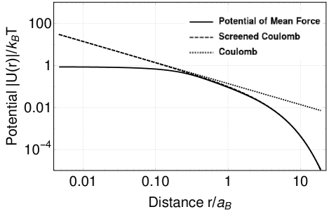
Figure 2: Example electron-deuteron scattering potentials in classical, weakly coupled regime $T=300{\rm eV}$ and $n=5.3\times 10^{23}{\rm cm}^{-3}$, for which $\Theta=13$ and $\Gamma_{e}=\Gamma_{i}=0.043$ (top) and degenerate, moderately-coupled regime with $T=3{\rm eV}$, $n=4.5\times 10^{23}$, for which $\Theta=0.14$, $\Gamma_{i}=4.1$ and $\Gamma_{e}=1.3$ (bottom). Here, $a_{B}$ is the Bohr radius. Solid line: potential of mean force; dashed line: screened Coulomb potential with screening length from equation (37); dotted line: bare Coulomb potential.

IV Transport Rates

IV.1 General Formalism

Temperature relaxation is a transport process of practical importance to WDM. It acts as a probe of electron-ion collisions in this environment, and the relaxation time $\tau$ serves as an important indicator of the underlying physics. WDM is often created in a state that is far from equilibrium. Due to the electron-ion mass ratio, electrons and ions quickly relax into separate populations at two different temperatures. Electron-ion scattering then more slowly equilibrates the two temperatures. The rate $\tau$ is additionally an experimentally accessible parameter. Recent experiments have begun measuring this relaxation in the WDM regime (Cho et al., 2016; Zaghoo et al., 2019), and are showing interesting effects due to both degeneracy and Coulomb coupling. Electron-ion relaxation has been difficult to address computationally as a consequence of the mass ratio along with degeneracy and correlation. However, recent advances have been made to finally make reliable predictions of relaxation rates using wave packet molecular dynamics (Ma et al., 2019) and mixed classical-quantum molecular dynamics (Simoni and Daligault, 2019; Daligault and Mozyrsky, 2018). These methods are opening the door for unprecedented validation of analytical and numerical models. Theoretical prediction of relaxation in a plasma is typified by the theory of Landau and Spitzer. The Landau-Spitzer (LS) theory depends on the Coulomb logarithm $\ln\Lambda_{ei}$, which vanishes in dense plasmas when the screening length becomes smaller than the Wigner-Seitz radius $a$. Current models of temperature relaxation include the Fermi Golden Rule (FGR) method (Hazak et al., 2001; Dharma-wardana and Perrot, 1998), a standard plasma approach using the quantum Landau equation (Daligault, 2016), a method based on a quantum field theory for plasmas (Brown et al., 2005; Brown and Singleton, 2007; Singleton, 2007), and an approach that incorporates correlation effects in a normal mode kinetic calculation through including local field corrections (LFCs) in the dielectric response (Daligault and Dimonte, 2009), and the quantum Lenard-Balescu equation (Benedict et al., 2012; Scullard et al., 2018). Finally, a new method provides the relaxation rate in terms of the electron-ion collision cross section (Daligault and Simoni, 2019) and allows for both degeneracy and correlation in a large area of parameter space. This approach treats the ions as classical particles obeying a Langevin-like equation while the populations of the electron states obey a master equation, with relaxation rates determined from the frictional forces felt by the ions.

Momentum relaxation is another important process in dense plasmas. A velocity drift between electron and ion populations gives rise to a current, and electron-ion collisional friction contributes to the conductivity. While it should be noted that electron-electron collisions also contribute in calculations of the conductivity, in certain regimes the electron-ion collisions are dominant. LS theory again provides the conductivity for a classical plasma, but neglects both correlation and quantum effects. To correct for this, Lee and More introduced a transport model attempting to extend LS theory to regimes with strong coupling and degeneracy (Lee and More, 1984). The quantum LFP equation has been applied to the calculation of momentum relaxation as well (Daligault, 2016). However, these methods do not accurately account for strong collisions. The effects of strong collisions with diffraction on temperature relaxation have been addressed by the so-called T-matrix approach, but without incorporating degeneracy (Gericke et al., 2002). Degeneracy has been addressed through a variety of methods. The quantum Lenard-Balescu equation has been applied to electrical conductivity (Lampe, 1968), but again is limited to weak coupling. A model for conductivity in a degenerate and strongly-coupled plasma was obtained via the Kubo-Greenwood formalism combined with an average-atom two-component plasma model, where the degeneracy is included through its influence on the electron-ion potential (Starrett, 2018; Gill and Starrett, 2019).

A binary mixture of two species $s$ and $s^{\prime}$ out of equilibrium will relax towards equilibrium through $s-s$, $s-s^{\prime}$ and $s^{\prime}-s^{\prime}$ collisions, which are modeled by the collision operator (34). Specifically, taking velocity moments of the kinetic equation produces a hierarchy of fluid equations which can be closed through a perturbative expansion about equilibrium. Transport coefficients are determined from moments of the collision operator. The relevant moments can be written

$$\left\langle\chi_{l}\right\rangle^{s-s^{\prime}}=\int d\boldsymbol{v}\chi\left(\boldsymbol{v}\right)C_{qB}^{s-s^{\prime}},$$ (38)

where $\chi(\boldsymbol{v})$ is some polynomial function of the velocity. To simplify we utilize the following properties: $d\Omega\frac{d\sigma}{d\Omega}$ is invariant under reversal of the collision, i.e. $\left(\boldsymbol{\boldsymbol{v}},\boldsymbol{v}^{\prime}\right)\leftrightarrow\left(\hat{\boldsymbol{v}},\hat{\boldsymbol{v}}^{\prime}\right)$ where $\boldsymbol{\boldsymbol{v}}\thinspace{\rm and\thinspace}\boldsymbol{v}^{\prime}$ are the pre-collision velocities of particles one and two respectively and the “hat” $\hat{}$ indicates a post-collision quantity, and the phase-space volume element is invariant, i.e. $\int d\boldsymbol{v}d\boldsymbol{v}^{\prime}=\int d\hat{\boldsymbol{v}}d\hat{\boldsymbol{v}^{\prime}}$. We thus obtain

$$\left\langle\chi_{l}\right\rangle^{s-s^{\prime}}=\int d\boldsymbol{v}\int d\Omega\frac{d\sigma}{d\Omega}u\int d\boldsymbol{v}^{\prime}\left[\chi\left(\hat{\boldsymbol{v}}\right)-\chi\left(\boldsymbol{v}\right)\right]$$

$$\times f_{s}f_{s^{\prime}}\left(1+\theta_{s}\hat{f_{s}}\right)\left(1+\theta_{s}\hat{f_{s^{\prime}}}\right).$$ (39)

Relevant $\chi\left(v\right)$ are

$$\chi\left(\boldsymbol{v}\right)=\begin{cases}1\thinspace\thinspace\thinspace\thinspace\thinspace\thinspace\thinspace\thinspace\thinspace\rightarrow&\left[\chi\left(\hat{\boldsymbol{v}}\right)-\chi\left(\boldsymbol{v}\right)\right]=0\\ m_{s}\boldsymbol{v}\thinspace\rightarrow&\left[\chi\left(\hat{\boldsymbol{v}}\right)-\chi\left(\boldsymbol{v}\right)\right]=m_{s}\boldsymbol{\Delta}v\\ m_{s}v^{2}\rightarrow&\left[\chi\left(\hat{\boldsymbol{v}}\right)-\chi\left(\boldsymbol{v}\right)\right]=m_{s}\Delta v^{2}\end{cases}$$ (40)

where $\Delta\boldsymbol{v}=\hat{\boldsymbol{v}}-\boldsymbol{v}$. Substituting variables $\boldsymbol{v}=\boldsymbol{v}^{\prime}+\boldsymbol{u}$ and the collision kinematics which determine

$$m_{s}\Delta\boldsymbol{v}=m_{ss^{\prime}}\Delta\boldsymbol{u},$$ (41)

$$\Delta\boldsymbol{u}\cdot\Delta\boldsymbol{u}=-2\boldsymbol{u}\cdot\Delta\boldsymbol{u}$$ (42)

and

$$\left(2\boldsymbol{v}\cdot\Delta\boldsymbol{v}+\Delta\boldsymbol{v}^{2}\right)=\frac{m_{ss^{\prime}}}{m_{s}}\Delta\boldsymbol{u}\cdot\left(\boldsymbol{v}^{\prime}+\frac{m_{ss^{\prime}}}{m_{s}}\boldsymbol{u}\right),$$ (43)

(see (Baalrud, 2012)) shows that

$$\chi\left(\boldsymbol{v}\right)=\begin{cases}1\thinspace\thinspace\thinspace\thinspace\thinspace\thinspace\thinspace\thinspace\thinspace\rightarrow&\left[\chi\left(\hat{\boldsymbol{v}}\right)-\chi\left(\boldsymbol{v}\right)\right]=0\\ m_{s}\boldsymbol{v}\thinspace\rightarrow&\left[\chi\left(\hat{\boldsymbol{v}}\right)-\chi\left(\boldsymbol{v}\right)\right]=m_{ss^{\prime}}\Delta\boldsymbol{u}\\ m_{s}v^{2}\rightarrow&\left[\chi\left(\hat{\boldsymbol{v}}\right)-\chi\left(\boldsymbol{v}\right)\right]=m_{ss^{\prime}}\left(\boldsymbol{v^{\prime}}-\boldsymbol{V}_{s}+\frac{m_{ss^{\prime}}}{m_{s^{\prime}}}\boldsymbol{u}\right)\cdot\Delta\boldsymbol{u}\end{cases}$$ (44)

where

$$\Delta\boldsymbol{u}=u\left({\rm sin}\theta{\rm cos}\phi\hat{\boldsymbol{x}}+{\rm sin}\theta{\rm sin}\phi\hat{\boldsymbol{y}}-2{\rm sin}^{2}\frac{\theta}{2}\hat{\boldsymbol{u}}\right).$$ (45)

The preceding discussion and the collision operator (34) are in principle applicable to transport in any semi-classical system. As it pertains to WDM, ion-ion scattering is contained within this formalism as ion dynamics are classical and electron degeneracy effects enter only via the potential of mean force. Application of the theory to ion-ion scattering was validated in (Daligault et al., 2016). The case of the electron-electron terms requires further work due to the subtleties discussed at the end of section II. The model at the level to which we have developed it has immediate applicability to the case of electron-ion scattering.

IV.2 The Relaxation Problem

Presently, we restrict our analysis to the class of problems in which electrons and ions in the plasma are in respective equilibrium with themselves with different fluid quantities $T_{e},\thinspace T_{i},\thinspace\boldsymbol{V}_{e}\thinspace{\rm and}\thinspace\boldsymbol{V}_{i}$, respectively. In such a system, the electron and ion fluid variables will equilibrate on a timescale long compared to the respective electron-electron and ion-ion collision times. The ions have a classical Maxwellian velocity distribution

$$f_{i}\left(\boldsymbol{v}^{\prime}\right)=\frac{n_{i}}{v_{Ti}^{3}}\frac{e^{-\left(\boldsymbol{v}^{\prime}-\boldsymbol{V}_{i}\right)^{2}/v_{Ti}^{2}}}{\pi^{3/2}}$$ (46)

and the electrons have an appropriately normalized Fermi-Dirac velocity distribution

$$f_{e}\left(\boldsymbol{v}\right)=n_{e}\left[v_{Te}^{3}\left(-\pi^{3/2}\text{Li}_{\frac{3}{2}}(-\xi)\right)\left(1+\frac{{\rm e}^{\left(\boldsymbol{v}-\boldsymbol{V}_{e}\right)^{2}/v_{Te}^{2}}}{\xi}\right)\right]^{-1}$$ (47)

where $v_{Ts}=\sqrt{2k_{B}T_{s}/m_{s}}$ and $\xi=\exp\left(\mu/k_{B}T\right)$, the ion velocity is $\boldsymbol{v^{\prime}}$ and electron velocity is $\boldsymbol{v}$. We can write

$$f_{e}f_{i}\left(1+\theta_{e}\hat{f_{e}}\right)=\frac{n_{i}}{v_{Ti}^{3}}\frac{e^{-\left(\boldsymbol{v}^{\prime}-\boldsymbol{V}_{i}\right)^{2}/v_{Ti}^{2}}}{\pi^{3/2}}n_{e}$$

$$\times\left[v_{Te}^{3}\left(-\pi^{3/2}\text{Li}_{\frac{3}{2}}(-\xi)\right)\left(1+\frac{{\rm e}^{\left(\boldsymbol{v}-\boldsymbol{V}_{e}\right)^{2}/v_{Te}^{2}}}{\xi}\right)\right]^{-1}$$

$$\times\left[1-\left(1+\frac{{\rm e}^{\left(\boldsymbol{v}+\Delta\boldsymbol{v}-\boldsymbol{V}_{e}\right)^{2}/v_{Te}^{2}}}{\xi}\right)^{-1}\right],$$ (48)

from which the relation of the factor $\left(1+\theta_{e}\hat{f_{e}}\right)$ to Pauli blocking can be seen in terms of the Fermi-Dirac occupation number: the contribution to the collision integral from collisions to or from occupied states is zero. This simplification occurs from the combination of $\theta_{e}$ with the Fermi Dirac distribution and the relation (3).

Electron-ion temperature and momentum relaxation rates depend on the energy exchange density $Q^{s-s^{\prime}}$ and friction force density $\boldsymbol{R}^{s-s^{\prime}}$, respectively. These can in turn be written in terms of the moments (39), assuming a uniform plasma, as

$$Q^{ei}=\left\langle\frac{1}{2}m_{e}\left(\boldsymbol{v}-\boldsymbol{V}_{e}\right)^{2}\right\rangle^{e-i}=\frac{3n_{e}}{2}\frac{dT_{e}}{dt}$$ (49)

(where in the last equality we have taken $\boldsymbol{V}_{e}=\boldsymbol{V}_{i}=0)$ and

$$\boldsymbol{R}^{ei}=\left\langle m_{e}\boldsymbol{v}\right\rangle^{e-i}=m_{e}d\left\langle\boldsymbol{v}\right\rangle/dt=m_{e}\frac{d\boldsymbol{V}_{e}}{dt}$$ (50)

which, in the respective limits of $\Delta T\ll T$ and $\Delta V\ll V$ yield simple relaxation rates $dT_{e}/dt=\nu_{ei}^{(\epsilon)}\Delta T$ and $d\boldsymbol{V}_{e}/dt=\nu_{ei}^{(p)}\Delta\boldsymbol{V}$.

The integration over the ion velocity can be simplified significantly in the limit that the ion velocities are much smaller than the electron velocities: $m_{e}T_{i}\ll m_{i}T_{e}$, which is true when temperature differences are not extreme, which coincides with our expansion about the equilibrium state. By expanding equation (48) in the limit that the electron distribution is approximately constant over the range of accessible ion velocities, the integral over the ion velocities can be carried out analytically. The evaluation of this integral differs for the calculation of $Q^{ei}$ versus $\boldsymbol{R}^{ei}$. Therefore we examine each case separately.

IV.2.1 Temperature Relaxation

The energy-exchange density (49) in this case becomes

$$Q^{ei}=\int d\boldsymbol{u}\int d\Omega\frac{d\sigma}{d\Omega}u\boldsymbol{\Delta u}$$

$$\cdot\int d\boldsymbol{v}^{\prime}m_{ei}\left(\boldsymbol{v^{\prime}}+\frac{m_{ei}}{m_{i}}\boldsymbol{u}\right)f_{i}f_{e}\left(1-|\theta|\hat{f_{e}}\right).$$

Inserting equation (48) and applying the expansion $|\boldsymbol{v}^{\prime}|\ll|\boldsymbol{u}|$ and assuming zero drift velocities and $\left|T_{e}-T_{i}\right|\ll T_{e},T_{i}$ we perform the integral over $\boldsymbol{v}^{\prime}$ and write

$$\boldsymbol{\Delta u}\cdot\int d\boldsymbol{v}^{\prime}m_{ei}\left(\boldsymbol{v^{\prime}}+\frac{m_{ei}}{m_{i}}\boldsymbol{u}\right)f_{i}f_{e}\left(1-|\theta|\hat{f_{e}}\right)\approx$$

$$\frac{n_{e}n_{i}\xi e^{-\eta^{2}}\sin^{2}\left(\frac{\theta}{2}\right)}{\pi^{3}v_{Te}\text{Li}_{\frac{3}{2}}\left(-\xi\right)\left(\xi e^{-\eta^{2}}+1\right)^{2}}$$

where $\eta\equiv u/v_{Te}$ and therefore obtain, written to facilitate comparison with the classical limit,

$$Q^{ei}=-3\frac{m_{e}}{m_{i}}n_{e}\nu_{ei}^{(\epsilon)}(T_{e}-T_{i}).$$ (51)

The collision frequency $\nu_{ei}^{(\epsilon)}$ can be written in terms of a reference frequency,

$$\nu_{0}\equiv\frac{4\sqrt{2\pi}n_{e}e^{4}}{3\sqrt{m_{e}}(k_{B}T_{e})^{3/2}}$$ (52)

and a generalized Coulomb integral $\Xi_{ei}^{(\epsilon)}$,

$$\nu_{ei}^{(\epsilon)}=\nu_{0}\Xi_{ei}^{(\epsilon)}.$$ (53)

Effects of degeneracy and strong coupling are contained in the function which replaces the Coulomb logarithm,

$$\Xi_{ei}^{(\epsilon)}=\frac{1}{2}\int_{0}^{\infty}d\eta G_{1}(\eta)\frac{\sigma_{1}^{(1)}\left(\eta,\Gamma\right)}{\sigma_{0}}$$ (54)

$$\equiv\frac{1}{2}\int_{0}^{\infty}d\eta I_{\epsilon}(\eta)$$

where

$$\sigma_{1}^{(1)}\left(\eta,\Gamma\right)=4\pi\int_{0}^{\pi}d\theta\sin^{2}\frac{\theta}{2}\sin\theta\frac{d\sigma}{d\Omega}$$ (55)

is the momentum transfer cross section, written in terms of the phase shifts $\delta_{l}$ as

$$\sigma_{1}^{(1)}=\frac{4\pi}{\eta^{2}}\sum_{l=0}^{\infty}(l+1)\sin^{2}(\delta_{l+1}-\delta_{l}).$$ (56)

The function

$$G_{1}(\eta)\equiv\frac{\xi{\rm e}^{-\eta^{2}}\eta^{5}}{\left[-\text{Li}_{\frac{3}{2}}\left(-\xi\right)\right]\left(\xi e^{-\eta^{2}}+1\right)^{2}}$$ (57)

determines the relative availability of states that contribute to the scattering. This is plotted in figure 3 for several values of the degeneracy parameter $\Theta$, where it is shown that in the classical limit scattering is dominated by energy transfers around the thermal energy, and as degeneracy increases the envelope of relevant momentum-transfers narrows about the Fermi momentum. It must be noted that the relaxation rate obtained is identical to that obtained in equation (71) of reference (Daligault and Simoni, 2019) by very different means, although the PMF does not appear naturally in this other formulation and must be manually included in the calculations of the cross sections.

IV.2.2 Momentum Relaxation

Electron-ion momentum relaxation is a major contributor to electrical resistivity, diffusion, and is also related to the stopping power of ions in a plasma. Here, we concentrate on the case that drift velocities are much slower than the electron thermal speed, with the goal of obtaining a relaxation rate rather than stopping power. Relaxation occurs through collisions between electron and ion populations with different average velocities. The force density (50) associated with these collisions is

$$\boldsymbol{R}^{ei}=\int d\boldsymbol{v}\int d\Omega\frac{d\sigma}{d\Omega}u\int d\boldsymbol{v}^{\prime}m_{ei}\boldsymbol{\Delta u}f_{e}f_{i}\left(1+\theta_{e}\hat{f_{e}}\right).$$ (58)

Inserting equation (48) into the above equation and applying the expansion $|\boldsymbol{v}^{\prime}|\ll|\boldsymbol{u}|$ and assuming $\left|T_{e}-T_{i}\right|\ll T_{e},T_{i}$ and $V_{i}\ll v_{Ti}$ and $V_{e}\ll v_{Te}$, the integral over $\boldsymbol{v}^{\prime}$ can be performed analytically and results in

$$\int d\boldsymbol{v}^{\prime}m_{ei}f_{e}f_{i}\left(1+\theta_{e}\hat{f_{e}}\right)$$

$$\approx\frac{2m_{e}n_{e}\xi n_{i}e^{-\eta^{2}}\left[\boldsymbol{u}\cdot\boldsymbol{\Delta V}-\xi e^{-\eta^{2}}\left(\boldsymbol{\Delta u}+\boldsymbol{u}\right)\cdot\boldsymbol{\Delta V}\right]}{\pi^{3/2}v_{Te}^{5}\left[-\text{Li}_{\frac{3}{2}}\left(-\xi\right)\right]\left(\xi e^{-\eta^{2}}+1\right){}^{3}}.$$

We follow the classical example and write

$$\boldsymbol{R}^{ei}=-n_{e}m_{e}\nu_{ei}^{(p)}(\boldsymbol{V}_{e}-\boldsymbol{V}_{i})$$ (59)

where the frequency

$$\nu_{ei}^{(p)}=\nu_{0}\Xi_{ei}^{(p)}$$ (60)

involves a Coulomb integral

$$\Xi_{ei}^{(p)}=\frac{1}{2}\int_{0}^{\infty}d\eta\left[G_{2}(\eta,\xi)\frac{\sigma_{1}^{(1)}\left(\eta,\Gamma\right)}{\sigma_{0}}-G_{3}(\eta,\xi)\frac{\sigma_{2}^{(1)}\left(\eta,\Gamma\right)}{\sigma_{0}}\right]$$

$$=\frac{1}{2}\int_{0}^{\infty}d\eta G_{2}(\eta,\xi)\frac{\sigma_{p}(\eta,\Gamma,\xi)}{\sigma_{0}}$$ (61)

$$\equiv\frac{1}{2}\int_{0}^{\infty}d\eta I_{p}(\eta,\Gamma,\xi),$$

which is different from that involved in the energy-exchange density. Here, $\sigma_{1}^{(1)}$ was defined previously and

$$\sigma_{2}^{(1)}\left(\eta,\Gamma\right)=4\pi\int_{0}^{\pi}d\theta\sin^{2}\frac{\theta}{2}\sin\theta\frac{d\sigma}{d\Omega}\cos\theta.$$ (62)

This differs from the classical case in which momentum and temperature relaxation differ only by a numerical factor and a mass ratio (Baalrud, 2012). The weighting functions

$$G_{2}(\eta,\xi)=\frac{\xi{\rm e}^{-\eta^{2}}\eta^{5}}{\left[-\text{Li}_{\frac{3}{2}}\left(-\xi\right)\right]\left(\xi e^{-\eta^{2}}+1\right)^{3}},$$ (63)

$$G_{3}(\eta,\xi)=\frac{\xi^{2}{\rm e}^{-2\eta^{2}}\eta^{5}}{\left[-\text{Li}_{\frac{3}{2}}\left(-\xi\right)\right]\left(\xi e^{-\eta^{2}}+1\right)^{3}},$$ (64)

are shown in figure 3 and compared with the statistical weighting factors in the case of temperature relaxation. The presence of the differing angular integrals between the energy and momentum relaxation cases warrants further discussion.

The function (62) behaves differently than a momentum transfer cross-section, and indeed can take on negative values. Through the use of the Wigner-3j function, $\sigma_{2}^{(1)}$ can be expanded in the phase shifts (see appendix B) as

$$\sigma_{2}^{(1)}=\frac{4\pi}{\eta^{2}}\sum_{l=0}^{\infty}\frac{\sin\delta_{l}}{4l(l+1)-3}$$

$$\times\left\{(l+1)(2l-1)\left[(l+2)\sin(\delta_{l}-2\delta_{l+2})-(2l+3)\sin(\text{$\delta_{l}$}-2\text{$\delta_{l+1}$})\right]-l^{2}(2l+3)\sin\delta_{l}\right\}.$$ (65)

While it is tempting to interpret the quantity $\sigma_{2}^{(1)}$ as a cross-section, $\sigma_{2}^{(1)}$ can become negative, and as will be shown in the following section, it is only in the combination $\sigma_{p}=\sigma_{1}^{(1)}\left(\eta,\Gamma\right)-\xi_{e}{\rm e}^{-\eta^{2}}\sigma_{2}^{(1)}\left(\eta,\Gamma\right)$ that this interpretation is justified. We thus refer to $\sigma_{p}$ as an effective transport cross section. We note that this second term arises due to degeneracy, and has no analog in the classical relaxation problem.

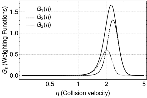
Figure 3: Statistical contributions to the integrands for temperature and momentum relaxation, $G_{1}$ (solid), $G_{2}$ (dashed) and $G_{3}$ (dotted), for three conditions: $\Theta=12.6$ and $\xi=0.017$ (top, weak degeneracy), $\Theta=0.85$ and $\xi=1.33$ (middle, moderate degeneracy), $\Theta=0.14$ and $\xi=1135$ (bottom, strong degeneracy). The relevant collision velocities for both momentum and temperature relaxation become narrowly centered around the Fermi velocity at strong degeneracy. The relative importance of the two different functions that contribute to momentum relaxation can be seen to depend on the degeneracy.

Figure 4: Top: Functions $\sigma_{1}^{(1)}$ (left) and $\sigma_{2}^{(1)}$ (right) calculated using the PMF (solid) and a screened Coulomb potential equation (36) (dashed) in the classical, weakly-coupled limit with $T=200\thinspace{\rm eV}$ and $n=0.774\thinspace{\rm g}\cdot{\rm cm}^{-3}$. Bottom: the same, but in the degenerate, moderately-coupled case with $T=3\thinspace{\rm eV}$ at the same density. This shows the different behaviors of the effective transport cross sections, and the breakdown of the screened Coulomb potential with the appearance of coupling effects at low temperature.

Figure 5: Integrands ($I_{\epsilon}(\eta)$ solid and $I_{p}(\eta)$ dashed) appearing in equations (54) and (61) for deuterium at $0.774\thinspace{\rm g\cdot cm}^{-3}$ at three different temperatures: $200\thinspace{\rm eV}$ ($\Theta\gg 1$) (top), $12\thinspace{\rm eV}$ ($\Theta\sim 1$) (middle), $3\thinspace{\rm eV}$ ($\Theta\ll 1$) (bottom).

V Relaxation Rates in Dense Deuterium Plasma

We illustrate the relaxation rates predicted by the quantum mean force theory for the case of dense deuterium with structural data provided by the average-atom two-component-plasma model (see (Starrett and Saumon, 2012, 2013)). We compare $\sigma_{2}^{(1)}$ with $\sigma_{1}^{(1)}$ in figure 4. The combined influence of the negative values of $\sigma_{2}^{(1)}$ and the preceding negative sign in equation (61) leads to interesting behavior in the integrand for the Coulomb integral. The full integrand of equation (61) is shown in figure 5 where it is seen that the resulting integrals are positive, as required. Note that the integrands are peaked functions; broad and peaked near the thermal velocity $v_{Ts}$ in the classical limit, and narrow with peak near the Fermi velocity in the degenerate limit. Also note that $I_{p}$ and $I_{\epsilon}$ are identical in the classical limit, but differ substantially in the degenerate case due to the presence of the $\sigma_{2}^{(1)}$ factor.

We proceed to use equations (51) and (59) to calculate relaxation rates for the case of deuterium compressed to $0.774$, $1.75$, and $20$ ${\rm g}\,{\rm cm}^{-3}$. So as to explore the parameter space targeted by our model; for each density we consider a range of temperatures so that the system ranges from classical and weakly coupled to degenerate with moderately coupled ions. The selected points can be seen in figure 1. We compare both the temperature and momentum relaxation rates to traditional weak-coupling models: the Landau-Spitzer rate, the quantum Landau-Fokker-Planck (LFP) rate (Daligault, 2016), and the Lee-More (LM) rate (Lee and More, 1984). These results are shown in figures 6-8.

Each model reproduces the well-established Landau-Spitzer result

$$\nu_{ei}^{{\rm LS}}=\nu_{0}\ln\Lambda$$ (66)

in the classical weakly-coupled limit. For a given density, the models diverge as temperature decreases and the threshold is crossed into either strong-coupling or degenerate regimes. For reference, we provide the scattering rates predicted by the LM and LFP theories here. The electrical conductivity coefficient predicted by the LM model (Lee and More, 1984) is

$$\sigma_{e}=\frac{ne^{2}}{m}\left\{\frac{3\sqrt{m}(kT)^{3/2}}{2\sqrt{2}\pi Z^{2}n_{i}e^{4}\ln\Lambda}\right\}\frac{4}{3}\frac{\int_{0}^{\infty}\frac{t^{3}dt}{1+\exp(t-\mu/kT)}}{\int_{0}^{\infty}\frac{t^{1/2}dt}{1+\exp(t-\mu/kT)}}$$ (67)

which is related to the friction force density $\boldsymbol{R}$ and thus the scattering rate: $\nu_{ei}^{(p)}=e^{2}n_{e}/\sigma m_{e}$ giving

$$\nu_{ei}^{{\rm LM}}=\nu_{0}\left[\ln\Lambda\frac{{\rm Li}_{3/2}(-\xi)}{{\rm Li}_{4}(-\xi)}\right].$$ (68)

The quantum LFP equation predicts a collision rate of (Daligault, 2016)

$$\nu_{ei}^{{\rm LFP}}=\nu_{0}\left(\ln\Lambda\frac{\xi}{1+\xi}\frac{3\sqrt{\pi}\Theta^{3/2}}{4}\right).$$ (69)

We further note our expression for the temperature relaxation rate (given by equations (51)-(56)) is the same as that recently obtained by a substantially different method as equations (71)-(75) by Daligault and Simoni (Daligault and Simoni, 2019). This equivalency can be seen through use of the relation $n_{e}\left(h/\sqrt{\pi}m_{e}V_{e}\right)^{3}=-2{\rm Li}_{3/2}\left(-\xi\right)$ from the normalization of the Fermi-Dirac distribution. We point out that the potential of mean force does not appear naturally in their expression but can be included ad-hoc in the calculation of the transport cross section.

The characteristic divergence of the Landau-Spitzer result due to the presence of the (inverse) Coulomb logarithm

$$\ln\Lambda_{{\rm LS}}=\ln\frac{b_{{\rm max}}}{b_{{\rm min}}},$$ (70)

restricts it from estimating transport even at moderate coupling. The maximum impact parameter is modeled as the larger of either the screening length $\lambda_{{\rm sc}}$ or the Wigner-Seitz radius $a=(3/4\pi n_{i})^{1/3}$, and the minimum is either the classical distance of closest approach $r_{L}=e^{2}/k_{B}T$, or more typically in dense plasmas the thermal de Broglie wavelength $\lambda_{{\rm dB}}=\hbar/\left(m_{e}k_{{\rm B}}T_{e}\right)^{1/2}$. In dense plasmas the vanishing Coulomb logarithm is often resolved through the modification (see e.g. (Lee and More, 1984))

$$\ln\Lambda_{{\rm LFP}}=\frac{1}{2}\ln\left(1+\frac{b_{{\rm max}}^{2}}{b_{{\rm min}}^{2}}\right),$$ (71)

which we apply in the LM and LFP cases. Furthermore in the LM model it is (artificially) enforced that the minimum value of the Coulomb logarithm be 2 (Lee and More, 1984):

$$\ln\Lambda_{{\rm LM}}={\rm max}\left[2,\frac{1}{2}\ln\left(1+\frac{b_{{\rm max}}^{2}}{b_{{\rm min}}^{2}}\right)\right].$$ (72)

The approximations inherent in this approach are two-fold: small-angle collisions must be assumed to obtain the LFP equation, and the choice of maximum and minimum impact parameters represents an uncontrolled expansion in the strongly coupled regime. The convergent kinetic equation in our approach avoids these limitations.

Temperature relaxation times are shown in figure 6 for compressed deuterium at $0.774,\thinspace 1.75\thinspace{\rm and}\thinspace 20\thinspace{\rm g}\cdot{\rm cm}^{-3}$. The potential of mean force force is calculated from pair distributions obtained via the average-atom/two-component plasma method of (Starrett and Saumon, 2012, 2013). The LS, LM and LFP rates are calculated according to equations (66)-(72). All expressions agree at high temperatures in the weakly-coupled classical regime, while at low temperature the models differ by a factor of $10^{2}-10^{3}$ as a result of the different levels of inclusion of the physics of strong coupling and degeneracy. In each case there is a minimum in the relaxation time. For the LS result this is a consequence of the disappearance of $\ln\Lambda$, indicating the transition to strong coupling. If the density is less than $10^{23}\thinspace{\rm cm}^{-3}$ this will occur at a temperature at which the plasma is not yet degenerate, and if the density is greater than $10^{23}\thinspace{\rm cm}^{-3}$ the electrons will be degenerate. However, in the other theories the minimum in $\tau$ persists, but is most prominent in the QMFKT while being least significant in the LM and LFP theories that do not account for strong coupling. This minimum can be attributed to a combination of both degeneracy and strong coupling.

At high temperatures, the plasma is classical and weakly coupled, and at low temperatures the plasma is degenerate and strongly coupled, while in between there is a mixture of moderate coupling and degeneracy effects. In order to assess the relative impact of large-angle collisions, correlations, Pauli blocking, and diffraction, we compare calculations with the following models: qLFP (no large-angle collisions or correlations), classical MFKT (no diffraction or Pauli blocking), quantum mean-force theory with classical scattering (no diffraction), quantum kinetic theory with a screened Yukawa potential (neglects strong correlations) and quantum mean-force theory with Maxwellian statistics (diffraction but no Pauli blocking), and finally the full QMFKT with degeneracy, diffraction, correlations and large-angle collisions included. We illustrate this comparison in figure 7 for the case of deuterium at $0.774\thinspace{\rm gpcc}$. Beginning with the full QMFKT, we can “turn off” various physical effects to determine their relative importance. For low-enough temperatures, the Pauli blocking contribution becomes significant as there is a large difference between the calculations with and without degeneracy, comparable to the difference between the weakly-coupled quantum LFP theory and the full QMFKT. The impact of diffraction continues to higher temperatures as can be seen in comparison of the calculations with quantum versus classical scattering. The relative importance of correlations and strong collisions vary depending on the density regime. At lower densities, both correlations and large-angle collisions become important at higher temperatures than the Fermi temperature; at higher densities strong collisions are suppressed by the Pauli blocking at all temperatures that would otherwise be strongly coupled. However, the correlations still persist at these densities and influence the scattering. Notably, the correlations and Pauli blocking both contribute to the increasing relaxation times at low temperature, as can be noted by comparison of the classical mean-force and the BUU with screened potential models which both flatten, with the combined effect in the full quantum mean-force model being a large increase in relaxation time at low temperatures. The BUU results with the screened Coulomb potential most closely resemble the LFP results as could be expected from the weak-coupling approximation. However, our method allows for large-angle collisions in addition to the correlations.

The relaxation time $\tau$ for energy and momentum relaxation are shown for compressed deuterium at three densities in figure 8. The rates are equal in the classical limit as expected, and differ for lower temperatures when degeneracy arises. The relaxation times differ for $T<T_{F}$, and notably the difference is larger for the higher density cases, even for similar levels of degeneracy $\Theta$. Generally, the rates are smaller for energy relaxation, with the maximum difference being a factor of $\sim 2$ at the lowest density $0.774\thinspace{\rm g}\cdot{\rm cm}^{-3}$ and only slightly larger at the higher densities. It is unclear whether the collision frequencies themselves differ for the case of different electron and ion temperatures versus different drift velocities. This could be clarified through a more general calculation of relaxation in a plasma with both different electron/ion temperatures and drift velocities. Experimental validation of this phenomenon will require accurate measurements of both momentum and temperature relaxation rates in WDM, a matter of considerable difficulty. However, further consideration of the physical basis for the difference between momentum and temperature relaxation is called for, and perhaps computational methods will prove to be effective to this end.

VI Conclusions

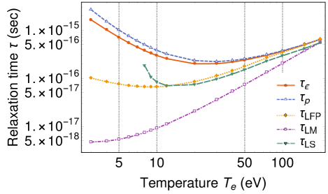
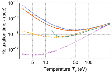
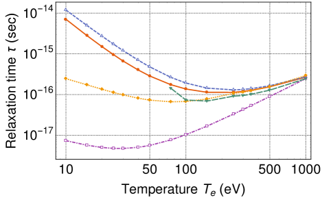
Figure 6: Electron-ion collisional relaxation times ($\tau=\nu_{ei}^{-1}$) as a function of temperature in deuterium at $0.774\thinspace{\rm g\cdot{\rm cm}^{-3}}$ (top), $1.75\thinspace{\rm g\cdot{\rm cm}^{-3}}$ (middle) and $20\thinspace{\rm g\cdot{\rm cm}^{-3}}$ (bottom).

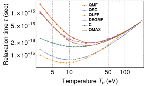
Figure 7: Comparison of temperature relaxation times from differing methods in order to elucidate the relative importance of Pauli blocking, correlations, large-angle scattering, and diffraction, for deuterium at $0.774\thinspace{\rm g\cdot cm}^{-3}$. The lines correspond to the different levels of evaluation of the collision operator in an attempt to “turn off” different combinations of physical processes: QMF (quantum mean-force kinetic theory), QSC (BUU with screened potential), QLFP (quantum LFP equation [screened potential with weak collisions]), DEGMF (QMFKT with the potential of mean force and classical scattering), C (fully-classical mean-force theory), and QMAX (mean-force theory with quantum scattering but Maxwellian statistics).

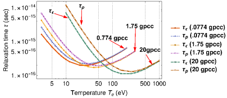
Figure 8: Comparison of temperature and momentum relaxation times in all three density regimes considered. In each case rates differ for $T<T_{F}$ but do not diverge widely even at very low temperature. The rates are smaller for temperature relaxation than for momentum relaxation.

We have presented a model for transport in plasmas with weak to moderate Coulomb coupling and weak to moderate electron degeneracy. The model is derived from the quantum BBGKY hierarchy with a closure scheme that expands about the deviation of correlations from their equilibrium values rather than in terms of the strength of the correlations. This incorporates correlations in the equilibrium limit while maintaining the simplicity of binary collisions in the dynamical equation. Although the expansion provides a general framework, it is difficult to solve in practice. A practical model was obtained by applying a quasi-classical approximation, closure at $n=2$, and the molecular chaos approximation. This is relevant to electron-ion collisions in warm dense matter. The result has the form of a Boltzmann-Uehling-Uhlenbeck equation, but where the binary collisions are mediated by the electron-ion potential of mean force (PMF), which is calculated directly from the pair distribution function $g_{ei}(r).$ Any means of obtaining $g_{ei}$ thus provides a means of obtaining the PMF.

The model was used to evaluate relaxation rates in warm dense deuterium, in which the $g_{ei}$ were provided by an average-atom two-component-plasma hybrid model (Starrett and Saumon, 2012). The temperature relaxation rate was written analogously to the classical Landau-Spitzer (LS) result in terms of a “Coulomb integral” that takes the place of the traditional Coulomb logarithm. The Coulomb integral for temperature relaxation depends on the level of degeneracy, and Coulomb coupling enters through the calculation of the momentum-transfer cross section solving the Schrödinger equation with the PMF as the scattering potential. The momentum relaxation rate differs from temperature relaxation in that it depends on a different transport cross section, which includes a term that is solely associated with degeneracy, and has no analog in the classical limit. The dependence of the integrands of the Coulomb integrals on the level of degeneracy was compared for the temperature and momentum relaxation cases.

We concluded by calculating the temperature and momentum relaxation rates in dense deuterium at three different densities over temperature ranges to cover the transitions between weak and moderate coupling and weak and moderate degeneracy. The temperature and momentum relaxation rates were compared with each other, and also compared with other common approximations for the relaxation rates. It was found that all models agree in the classical weak-coupling limit as expected, and diverge widely in the limit of a degenerate moderately-coupled plasma. We assessed the relative importance of the different relevant physical processes that complicate the problem as degeneracy and coupling simultaneously increase: diffraction, Pauli blocking, correlations, and large-angle scattering. Interestingly, in the degenerate regime there is a quantitative difference in the predicted relaxation rates for momentum versus energy. Ultimately, current and near-future experimental measurements and ab-initio simulations will be able to shed light on the applicability of the different models of transport for dense plasmas and WDM.

Further extensions of this work may be possible by solving the general formulation, rather than the semiclassical limit, to address electron-electron collisions in WDM. In this case the definition and interpretation of the PMF is complicated by both the exclusion and uncertainty principles. Further work will be required to obtain a rigorously derived convergent kinetic equation for electron-electron collisions. Finally, recent and upcoming experimental measurements of electrical conductivity and temperature relaxation (Cho et al., 2016; Zaghoo et al., 2019) may soon open the door for discrimination between the validity of the various models of relaxation in dense plasmas. This will enhance our understanding of the basic physics of dense plasmas, and allow increased fidelity in the rapid calculation of transport coefficients for use in hydrodynamic simulations of naturally and experimentally occurring WDM.

Appendix A Wigner Functions in The Wigner-Kirkwood Expansion

The reduced Wigner functions can be expressed in the semi-classical Wigner-Kirkwood expansion (Shalitin, 1973) as

$$f_{0}^{(n)}=\exp\left(-\frac{\beta}{2m}\sum_{i}^{n}p_{i}^{2}\right)\int d\boldsymbol{r}^{(N-n)}\exp\left(-\beta U\right)$$

$$\times\Bigg{\{}1+\hbar^{2}\beta^{2}\Bigg{[}-\frac{1}{24m}\sum_{i>n}\frac{\partial^{2}U}{\partial\boldsymbol{r}_{i}^{2}}$$

$$-\frac{1}{8m}\sum_{i\leq n}\frac{\partial^{2}U}{\partial\boldsymbol{r}_{i}^{2}}+\frac{\beta}{24m}\sum_{i\leq n}\left(\frac{\partial U}{\partial\boldsymbol{r}_{i}}\right)^{2}$$

$$+\frac{\beta}{24m^{2}}\sum_{i_{1}<n}\sum_{i_{2}\leq n}\frac{\partial^{2}U}{\partial\boldsymbol{r}_{i_{1}}\partial\boldsymbol{r}_{i_{2}}}:\boldsymbol{p}_{i_{1}}\boldsymbol{p}_{i_{2}}\Bigg{]}\Bigg{\}},$$

in which $\beta\equiv 1/k_{B}T$. Defining

$$C_{n}=\exp\left(-\frac{\beta}{2m}\sum_{i}^{n}p_{i}^{2}\right)\int d\boldsymbol{r}^{(N-n)}\exp\left(-\beta U\right)$$

$$Q_{n}=\hbar^{2}\beta^{2}\exp\left(-\frac{\beta}{2m}\sum_{i}^{n}p_{i}^{2}\right)\int d\boldsymbol{r}^{(N-n)}\exp\left(-\beta U\right)$$

$$\times\Bigg{[}-\frac{1}{24m}\sum_{i>n}\frac{\partial^{2}U}{\partial\boldsymbol{r}_{i}^{2}}-\frac{1}{8m}\sum_{i\leq n}\frac{\partial^{2}U}{\partial\boldsymbol{r}_{i}^{2}}+\frac{\beta}{24m^{2}}\sum_{i\leq n}\left(\frac{\partial U}{\partial\boldsymbol{r}_{i}}\right)^{2}$$

$$+\frac{\beta}{24m^{2}}\sum_{i_{1}<n}\sum_{i_{2}\leq n}\frac{\partial^{2}U}{\partial\boldsymbol{r}_{i_{1}}\partial\boldsymbol{r}_{i_{2}}}:\boldsymbol{p}_{i_{1}}\boldsymbol{p}_{i_{2}}\Bigg{]}$$

we can write

$$\frac{f_{0}^{(3)}}{f_{0}^{(2)}}=\frac{C_{3}+Q_{3}}{C_{2}+Q_{2}}$$ (73)

and, taking the expansion terms $Q_{n}$ to be small compared to the $C_{n}$, obtain

$$\frac{f_{0}^{(3)}}{f_{0}^{(2)}}\approx\exp\left(-\frac{\beta}{2m}p_{3}^{2}\right)\frac{g_{3}}{g_{2}}\left[1+\left(\frac{Q_{3}}{C_{3}}-\frac{Q_{2}}{C_{2}}\right)\right],$$ (74)

where $g_{3}=\int\exp\left(-\beta U\right)d^{3(N-3)}r$. The term in parenthesis is the first-order quantum correction, it is suppressed for small coupling and for small degeneracy. For the case of electron-ion collisions it can be neglected if both the degeneracy and coupling are only small to moderate. Dropping this term we obtain equation (24).

Appendix B Simplification of Cross Sections

Cross sections are calculated in the partial wave expansion

$$\frac{d\sigma}{d\Omega}=\left|\frac{1}{2ik}\sum_{l=0}^{\infty}\left(2l+1\right)\left({\rm e}^{2i\delta_{l}}-1\right)P_{l}\left({\rm cos}\theta\right)\right|^{2},$$ (75)

where the phase shifts $\delta_{l}$ are calculated from solution of the Schrödinger equation for the given potential. This can be written as a double sum

$$\frac{d\sigma}{d\Omega}=\frac{1}{k^{2}}\sum_{n=0}^{\infty}\sum_{m=0}^{\infty}\left(2m+1\right)\left(2n+1\right)$$

$$\times{\rm e}^{i\left(\delta_{m}-\delta_{n}\right)}\sin\delta_{m}\sin\delta_{n}{\rm P}_{m}(\cos\theta){\rm P}_{n}(\cos\theta)$$

which inserted into equation (62) results in

$$\sigma_{2}^{(1)}\left(\eta,\Gamma\right)=\frac{4\pi}{k^{2}}$$

$$\times\sum_{n=0}^{\infty}\sum_{m=0}^{\infty}\left(2m+1\right)\left(2n+1\right){\rm e}^{i\left(\delta_{m}-\delta_{n}\right)}\sin\delta_{m}\sin\delta_{n}$$

$$\times\int_{0}^{\pi}d\theta\sin^{2}\frac{\theta}{2}\sin\theta\cos\theta{\rm P}_{m}(\cos\theta){\rm P}_{n}(\cos\theta).$$

Taking advantage of the properties of the Legendre polynomials this is

$$\frac{4\pi}{k^{2}}\sum_{n=0}^{\infty}\sum_{m=0}^{\infty}\left(2m+1\right)\left(2n+1\right){\rm e}^{i\left(\delta_{m}-\delta_{n}\right)}\sin\delta_{m}\sin\delta_{n}$$

$$\times\frac{1}{2}\int_{0}^{\pi}\sin\theta\left[P_{1}(\cos\theta)-\frac{2}{3}P_{2}(\cos\theta)-\frac{P_{0}}{3}\right]$$

$$\times P_{m}(\cos\theta)P_{n}(\cos\theta)d\theta,$$

Finally, with the identity

$$\int_{0}^{\pi}d\theta\sin\theta P_{l}(\cos\theta)P_{m}(\cos\theta)P_{n}(\cos\theta)=2\left(\begin{array}[]{ccc}l&m&n\\ 0&0&0\end{array}\right)^{2},$$ (76)

where $\left(\begin{array}[]{c}\cdots\\ \cdots\end{array}\right)$ is the Wigner 3j symbol and using the specific values for $l=0,\thinspace 1,\thinspace{\rm and}\thinspace 2$, we obtain equation (65).

References

- Glenzer et al. (2016) S. H. Glenzer, L. B. Fletcher, E. Galtier, B. Nagler, R. Alonso-Mori, B. Barbrel, S. B. Brown, D. A. Chapman, Z. Chen, C. B. Curry, F. Fiuza, E. Gamboa, M. Gauthier, D. O. Gericke, A. Gleason, S. Goede, E. Granados, P. Heimann, J. Kim, D. Kraus, M. J. MacDonald, A. J. Mackinnon, R. Mishra, A. Ravasio, C. Roedel, P. Sperling, W. Schumaker, Y. Y. Tsui, J. Vorberger, U. Zastrau, A. Fry, W. E. White, J. B. Hasting, and H. J. Lee, Journal of Physics B Atomic Molecular Physics 49, 092001 (2016).
- Riley (2018) D. Riley, Plasma Physics and Controlled Fusion 60, 014033 (2018).
- Mančić (2010) A. Mančić, in Journal of Physics Conference Series, Vol. 257 (2010) p. 012009.
- Redmer et al. (2008) R. Redmer, N. Nettelmann, B. Holst, A. Kietzmann, and M. French, “Quantum Molecular Dynamics Simulations for Warm Dense Matter and Applications in Astrophysics,” in Condensed Matter Physics in the Prime of 21st Century: Phenomena, Materials, Ideas, Methods - 43rd Karpacz Winter School of Theoretical Physics (World Scientific Publishing Co. Pte. Ltd., 2008) pp. 223–236.
- Koenig et al. (2005) M. Koenig, A. Benuzzi-Mounaix, A. Ravasio, T. Vinci, N. Ozaki, S. Lepape, D. Batani, G. Huser, T. Hall, D. Hicks, A. MacKinnon, P. Patel, H. S. Park, T. Boehly, M. Borghesi, S. Kar, and L. Romagnani, Plasma Physics and Controlled Fusion 47, B441 (2005).
- Hu et al. (2015) S. X. Hu, V. N. Goncharov, T. R. Boehly, R. L. McCrory, S. Skupsky, L. A. Collins, J. D. Kress, and B. Militzer, Physics of Plasmas 22, 056304 (2015).
- Baalrud and Daligault (2019) S. D. Baalrud and J. Daligault, Physics of Plasmas 26, 082106 (2019), https://doi.org/10.1063/1.5095655 .
- Baalrud and Daligault (2013) S. D. Baalrud and J. Daligault, Physical Review Letters 110, 235001 (2013), arXiv:1303.3202 [physics.plasm-ph] .
- Baalrud and Daligault (2014) S. D. Baalrud and J. Daligault, Physics of Plasmas 21, 055707 (2014), arXiv:1403.1882 [physics.plasm-ph] .
- Daligault et al. (2016) J. Daligault, S. D. Baalrud, C. E. Starrett, D. Saumon, and T. Sjostrom, Physical Review Letters 116, 075002 (2016).
- Melrose and Mushtaq (2010) D. B. Melrose and A. Mushtaq, Phys. Rev. E 82, 056402 (2010).
- Daligault (2016) J. Daligault, Physics of Plasmas 23, 032706 (2016).
- Daligault (2018) J. Daligault, Physics of Plasmas 25, 082703 (2018), https://doi.org/10.1063/1.5045330 .
- Gericke et al. (2002) D. O. Gericke, M. S. Murillo, and M. Schlanges, Phys. Rev. E 65, 036418 (2002).
- Lee and More (1984) Y. T. Lee and R. M. More, Physics of Fluids 27, 1273 (1984).
- Starrett (2018) C. E. Starrett, Physics of Plasmas 25, 092707 (2018), arXiv:1808.07153 [physics.plasm-ph] .
- Daligault and Dimonte (2009) J. Daligault and G. Dimonte, Phys. Rev. E 79, 056403 (2009), arXiv:0902.1997 [physics.plasm-ph] .
- Lampe (1968) M. Lampe, Phys. Rev. 170, 306 (1968).
- Scullard et al. (2018) C. R. Scullard, S. Serna, L. X. Benedict, C. L. Ellison, and F. R. Graziani, Phys. Rev. E 97, 013205 (2018), arXiv:1710.00972 [physics.plasm-ph] .
- Brown et al. (2005) L. S. Brown, D. L. Preston, and R. L. Singleton, Jr., Physics Reports 410, 237 (2005), arXiv:physics/0501084 [physics.plasm-ph] .
- Brown and Singleton (2007) L. S. Brown and R. L. Singleton, Jr., Phys. Rev. E 76, 066404 (2007), arXiv:0707.2370 [physics.plasm-ph] .
- Singleton (2007) J. Singleton, Robert L., arXiv e-prints , arXiv:0706.2680 (2007), arXiv:0706.2680 [physics.plasm-ph] .
- Balzer and Bonitz (2013) K. Balzer and M. Bonitz, Nonequilibrium Green’s Functions Approach to Inhomogeneous Systems, Vol. 867 (2013).
- Bonitz (2016) M. Bonitz, Quantum Kinetic Theory (2016).
- Imam-Rahajoe and Curtiss (1967) S. Imam-Rahajoe and C. F. Curtiss, Journal of Chemical Physics 47, 5269 (1967).
- Hoffman et al. (1965) D. K. Hoffman, J. J. Mueller, and C. F. Curtiss, Journal of Chemical Physics 43, 2878 (1965).
- Hansen and McDonald (2006) J. Hansen and I. McDonald, Theory of Simple Liquids, 3rd ed. (Academic Press, Oxford, 2006).
- Shalitin (1973) D. Shalitin, J. Chem. Phys. 58, 5120 (1973).
- Grad (1958) H. Grad, Handbuch der Physik, Vol. Vol. 1 (Springer-Verlag, Berlin, 1958).
- Uehling and Uhlenbeck (1933) E. A. Uehling and G. E. Uhlenbeck, Physical Review 43, 552 (1933).
- Ross and Kirkwood (1954) J. Ross and J. G. Kirkwood, J. Chem. Phys. 22, 1094 (1954).
- Snider et al. (1995) R. F. Snider, W. J. Mullin, and F. Laloë, Physica A Statistical Mechanics and its Applications 218, 155 (1995).
- Boercker and Dufty (1979) D. B. Boercker and J. W. Dufty, Annals of Physics 119, 43 (1979).
- Landau and Lifshitz (1965) L. D. Landau and E. M. Lifshitz, Quantum mechanics (1965).
- Starrett and Saumon (2013) C. E. Starrett and D. Saumon, Phys. Rev. E 87, 013104 (2013).
- Shaffer and Baalrud (2019) N. R. Shaffer and S. D. Baalrud, Phys. Plasmas 26, 032110 (2019), arXiv:1902.02937 [physics.plasm-ph] .
- Starrett and Saumon (2012) C. E. Starrett and D. Saumon, Phys. Rev. E 85, 026403 (2012).
- Cho et al. (2016) B. I. Cho, T. Ogitsu, K. Engelhorn, A. A. Correa, Y. Ping, J. W. Lee, L. J. Bae, D. Prendergast, R. W. Falcone, and P. A. Heimann, Scientific Reports 6, 18843 (2016).
- Zaghoo et al. (2019) M. Zaghoo, T. R. Boehly, J. R. Rygg, P. M. Celliers, S. X. Hu, and G. W. Collins, Physical Review Letters 122, 085001 (2019), arXiv:1901.11410 [physics.plasm-ph] .
- Ma et al. (2019) Q. Ma, J. Dai, D. Kang, M. S. Murillo, Y. Hou, Z. Zhao, and J. Yuan, Phys. Rev. Lett. 122, 015001 (2019).
- Simoni and Daligault (2019) J. Simoni and J. Daligault, Phys. Rev. Lett. 122, 205001 (2019), arXiv:1904.04450 [physics.plasm-ph] .
- Daligault and Mozyrsky (2018) J. Daligault and D. Mozyrsky, Phys. Rev. B 98, 205120 (2018), arXiv:1708.06679 [physics.comp-ph] .
- Hazak et al. (2001) G. Hazak, Z. Zinamon, Y. Rosenfeld, and M. W. C. Dharma-wardana, Phys. Rev. E 64, 066411 (2001).
- Dharma-wardana and Perrot (1998) M. W. C. Dharma-wardana and F. Perrot, Phys. Rev. E 58, 3705 (1998).
- Benedict et al. (2012) L. X. Benedict, M. P. Surh, J. I. Castor, S. A. Khairallah, H. D. Whitley, D. F. Richards, J. N. Glosli, M. S. Murillo, C. R. Scullard, P. E. Grabowski, D. Michta, and F. R. Graziani, Phys. Rev. E 86, 046406 (2012).
- Daligault and Simoni (2019) J. Daligault and J. Simoni, Phys. Rev. E 100, 043201 (2019).
- Gill and Starrett (2019) N. M. Gill and C. E. Starrett, High Energy Density Physics 31, 24 (2019).
- Baalrud (2012) S. D. Baalrud, Physics of Plasmas 19, 030701 (2012).