A lazy decoder to reduce decoding hardware requirements for quantum computing

Hierarchical decoding to reduce hardware requirements for quantum computing

Abstract

Extensive quantum error correction is necessary in order to scale quantum hardware to the regime of practical applications. As a result, a significant amount of decoding hardware is necessary to process the colossal amount of data required to constantly detect and correct errors occurring over the millions of physical qubits driving the computation. The implementation of a recent highly optimized version of Shor’s algorithm to factor a 2,048-bits integer would require more 7 TBit/s of bandwidth for the sole purpose of quantum error correction and up to 20,000 decoding units.

To reduce the decoding hardware requirements, we propose a fault-tolerant quantum computing architecture based on surface codes with a cheap hard-decision decoder, the lazy decoder, combined with a sophisticated decoding unit that takes care of complex error configurations. Our design drops the decoding hardware requirements by several orders of magnitude assuming that good enough qubits are provided. Given qubits and quantum gates with a physical error rate $p=10^{-4}$, the lazy decoder drops both the bandwidth requirements and the number of decoding units by a factor 50x. Provided very good qubits with error rate $p=10^{-5}$, we obtain a 1,500x reduction in bandwidth and decoding hardware thanks to the lazy decoder.

Finally, the lazy decoder can be used as a decoder accelerator. Our simulations show a 10x speed-up of the Union-Find decoder and a 50x speed-up of the Minimum Weight Perfect Matching decoder.

Hundreds or thousands of high-quality qubits with an error rate of $10^{-10}$ or lower are necessary to implement quantum algorithms with industrial applications. In order to reach such high quality based on current quantum technology, logical qubits must be built from a large number of physical qubits and errors accumulating during the computation must be corrected at regular intervals.

The family of surface codes Dennis et al. (2002); Fowler et al. (2012a); Raussendorf and Harrington (2007); Fowler et al. (2009) is the most promising quantum error-correcting scheme to deal with current noise levels that barely reach $0.1\%$. Using a distance $d$ surface code, a logical qubit is encoded into a square grid of $d\times d$ data qubits as Fig. 2 shows. Error correction is based on the measurement of $r=d^{2}-1$ syndrome bits, extracted using syndrome measurement circuits implemented on the plaquettes of the qubit grid as shown in Fig. 2. The syndrome data is collected by the readout device and is sent to the decoding unit, which uses this information to detect and correct errors. In order to avoid accumulation of errors during the computation, the syndrome is constantly measured, producing $r$ syndrome bits for each syndrome measurement round. In the present work, we consider a syndrome measurement time of $1\mu s$, which is the time to implement the four rounds of CNOT gates and the final ancilla measurements of the syndrome measurement circuit. Consider as an example the recent RSA factorization algorithm of Gidney and Ekerå (2019), which relies on distance-27 surface codes, encoding $K\approx 10,000$ logical qubits (ignoring distillation qubits). The implementation of this algorithm requires a bandwidth of 7.3 TBit/s and two decoding units per logical qubit, that is 20,000 decoders, assuming independent correction of $X$-type and $Z$-type Pauli errors. It seems quite challenging to include such a formidable amount of decoding hardware to ensure fault tolerance in a quantum computer.

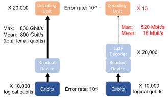
Figure 1: Left: Standard design with a readout device sending all syndrome data to the decoding unit. Two decoding units are used for each logical qubit, one for each type of error. Right: The readout device is equipped with a lazy decoder unit capable of correcting a large number of easy fault configurations, avoiding to transmit syndrome data to the decoding unit. We show the reduction in term bandwidth per logical qubit and number of decoding units obtained by introducing the lazy decoder in the case of physical error rate $p=10^{-5}$ with a logical error rate $p_{L}=10^{-15}$. In this case, including lazy decoding units, saves $99.9\%$ of the bandwidth requirement and $99.9\%$ of the complex decoding units.

In this work, we propose an alternative to the naive design that allocates one decoding unit for each decoding task by introducing a simple hard decision decoder, that we refer to as the lazy decoder. Fig. 1 illustrates our design and the saving obtained for a specific set of parameters. The lazy decoder can be seen as a pre-decoder which only attempt to correct easy error configurations. If no obvious correction exists, it quits and returns a failure mode. In that case, syndrome data is sent to a decoding unit that hosts a more sophisticated decoder achieving a good performance. Many complex decoding algorithms can play this role Dennis et al. (2002); Fowler et al. (2012b, c); Fowler (2015); Duclos-Cianci and Poulin (2010); Duclos-Cianci and Poulin (2013); Barrett and Stace (2010); Stace and Barrett (2010); Delfosse and Zémor (2017); Fowler (2013); Delfosse and Tillich (2014); Criger and Ashraf (2018); Nickerson and Brown (2019); Dennis (2005); Harrington (2004); Wootton and Loss (2012); Hutter et al. (2014); Wootton (2015); Herold et al. (2015); Breuckmann et al. (2016); Delfosse and Nickerson (2017); Tomita and Svore (2014); Heim et al. (2016); Torlai and Melko (2017); Baireuther et al. (2018); Krastanov and Jiang (2017); Varsamopoulos et al. (2017); Chamberland and Ronagh (2018); Breuckmann and Ni (2018); Sweke et al. (2018); Baireuther et al. (2019); Ni (2018); Andreasson et al. (2019); Davaasuren et al. (2018); Liu and Poulin (2019); Varsamopoulos et al. (2018, 2019); Wagner et al. (2019); Chinni et al. (2019); Sheth et al. (2019a); Colomer et al. (2019); Ferris and Poulin (2014); Bravyi et al. (2014); Darmawan and Poulin (2018); Tuckett et al. (2018)

The lazy decoder is designed to be as simple as possible. It consists of a single loop over syndrome bits, which makes it an ideal candidate for a low-level hardware implementation with FPGA or CMOS and it is also easy to parallelize. We picture the lazy decoder as a hardware unit, as close as possible to the readout device. In the worst case, we need two lazy decoder per logical qubit but given the speed of this module, one can expect sharing this unit between many of qubits. We assume that the measurement device (and therefore the lazy decoder) are placed in the proximity of the qubits in order to avoid long feedback loops increasing the physical qubit clock cycle.

The decoding unit, which is significantly more complex than the lazy decoder, may be challenging to implement close to the qubits without introducing additional noise to the quantum plane. Therefore, we consider a decoding unit placed at further distance from the qubits, which leads to latency issues, justifying our focus on the bandwidth of the readout-decoding unit link. We ignore the bandwidth between the readout-device and the adjacent lazy decoder.

Introducing the lazy decoder reduces the bandwidth required to send syndrome data from the readout device to the decoding unit because in most cases the nearby lazy decoder takes care of the correction. Moreover, the number of decoding units required is significantly reduced if one can rely on the lazy decoder a large fraction of the time. In what follows, we prove that this design leads to a reduction of the decoding hardware of several orders of magnitudes for good enough qubits. error rates below the standard assumption of $10^{-3}$.

I The surface code

The surface code encodes a logical qubit into a square grid of $d\times d$ data qubits where $d$ is the minimum distance of the code, as show in Fig. 2. Error correction relies on the syndrome measurement circuits represented in Fig. 2, consuming an additional $d^{2}-1$ qubits.

All plaquettes are measured simultaneously at regular intervals, producing rounds of syndrome data for the decoder which identifies errors based on this information. Fig. 2 shows the schedule used for the sequence of CNOT gates in order to allow for a parallel implementation and to preserve the code distance despite the propagation of errors by CNOT gates.

We simulate the surface code and the syndrome extraction circuit with a circuit level noise that represents imperfections on all qubits, gates, measurements, and waiting steps, by injecting random Pauli faults between any two steps of the circuit. A single qubit fault is included after each state preparation or waiting qubit with probability $p$. The Pauli fault is chosen uniformly in the set $\{X,Y,Z\}$. The outcome of a single qubit measurement is flipped with probability $2p/3$. The CNOT noise is modeled by a two-qubit Pauli fault injected after the CNOT with probability $p$. The fault is selected uniformly between the 15 non-trivial two-qubit Pauli operators acting on the support of the CNOT gate.

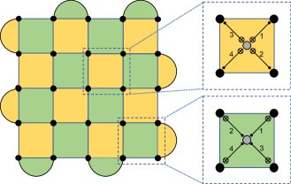
Figure 2: Distance five surface code with 25 (black) data qubits encoding 1 logical qubit. The measurement circuit on green and yellow plaquettes consume a (grey) ancilla qubit per plaquette. A syndrome extraction round is performed with three steps implemented simultaneously over all all the plaquettes: (i) Prepare the ancilla in the state $|+\rangle$ (green) or $|0\rangle$ (yellow). (ii) For each plaquette apply the four CNOT gates in the order prescribed by their indices, (iii) Measure the ancilla in the $Z$-basis (green) or in the $X$-basis (yellow). The final measurement produces a syndrome bit for each plaquette. Boundary plaquettes implement the restriction of the plaquette measurement circuit to two qubits.

Equipped with qubits and quantum gates affected by a circuit level noise with rate $p$, the surface code encoding provides a logical qubit whose error rate drops to Fowler et al. (2012a)

$$p_{L}(p,d)=0.1(100p)^{(d+1)/2}\cdot$$ (1)

where $d$ is the surface code minimum distance. One can use this heuristic formula to estimate the minimum distance $d$ required in order to achieve a given target logical error rate. Most practical applications necessitate a logical error rate that varies between $10^{-10}$ and $10^{-15}$, which is out of reach on current hardware without error correction.

Figure 3: A slice of the decoding graph obtained by placing a vertex in the center of each green plaquette and connecting incident plaquettes with an edge. A $Z$-fault is detected by either one or two plaquettes as shown with marked vertices.

After producing an encoded surface code state, we start measuring syndrome data. Non-trivial syndrome values indicate the presence of a fault. For simplicity, we focus on $Z$-type faults, detected by the measurement of green plaquettes as in Fig 3. $X$-type faults can be treated similarly. In what follows, we describe a graph that represents all possible faults in the syndrome measurement circuit. The whole simulation of the syndrome extraction circuit can be implemented based on this graph.

Consider the space-time locations $(x,y,t)$ of syndrome bits, where $(x,y)$ is the coordinates of the center of a plaquette and $t=0,1,2,\dots$ is the index of the syndrome round. Let $s(x,y,t)=0$ or $1$ be the syndrome value in location $(x,y,t)$. We record the changes of syndrome values, that is $\bar{s}(x,y,t)=s(x,y,t)-s(x,y,t-1)\pmod{2}$, and setting $\bar{s}(x,y,0)=0$ for the first round. A fault in the measurement circuit is detected by a set of syndrome locations $(x,y,t)$ where the syndrome value changes, i.e. $s(x,y,t)\neq 0$ A non-trivial fault is detected either in one location $u$ or in a pair of locations $u,v$, leading a natural graph structure.

The decoding graph represents all possible faults in the syndrome extraction circuit. The vertex set of the decoding graph is the set of syndrome locations. A half-edge $\{u,-\}$ or an edge $\{u,v\}$ is built from each potential fault in the syndrome extraction circuit. The decoding graph is a 3D cubic lattice with additional diagonal edges. Fig 3 shows a horizontal slice of the decoding graph. For each edge, we also store the probability of all circuit faults that map onto that edge. This edge weight can be processed by the decoder to provide a more accurate correction.

A surface code decoder takes as an input a set of consecutive rounds of syndrome data given by $\bar{s}$ and it aims at identifying the residual error on the $d^{2}$ data qubits. A standard decoding strategy consists in identifying a minimum set of edges that matches the observed syndrome $\bar{s}$.

II Lazy decoder

To simplify, we correct separately $X$-type and $Z$-type faults. Our objective is not to design a good decoder but to identify a set of fault configurations that is both very likely and easy to correct. The lazy decoder will correct exclusively this subset of easy configurations.

Let us first describe the most naive version of the lazy decoder. We simply check whether the syndrome is trivial and if so we send no data to the decoding unit. Clearly, it is easy to implement with low hardware costs. However, this does not help to reduce decoding hardware requirements since the probability to observed a trivial syndrome is generally too small. One could design a decoder that corrects any single fault or any fault of weight two, three and so on, but our numerical experiments show that either these sets of faults are still not likely enough for reasonable distances or the lazy decoder design becomes just as complex as the design of the whole decoding unit, defeating the whole purpose of the lazy decoder.

Algorithm 1 proposes a satisfying version of the lazy decoder for our architecture. We will prove that, when it succeeds, it returns a minimum set of faults explaining the syndrome observed. Our basic idea is to correct all configurations that can be corrected locally. This also guarantees a high potential for parallelism. If faults are sufficiently separated from each-other in space and time, we can obtain such a globally minimal solution from obvious locally optimal decisions.

The syndrome is given as an input of Algorithm 1 as a set of vertices $\bar{s}\subset V$ in the decoding graph induced by $Z$-type faults and the algorithm returns either an estimation ${\cal E}\subset E$ of the set of edges supporting faults, or a failure mode. The first block of Algorithm 1 looks for edges that match two neighbors syndrome bits $u,v\in\bf s$. Such an edge is locally optimal (it is the minimum number of faults explaining two non-trivial syndrome nodes) and can be safely added to the correction $\cal E$. The second block of Algorithm 1 takes care of remaining unmatched syndrome vertices, that come from faults on half-edges. The half-edge $\{u,-\}$ is a locally optimal choice to explain the non-trivial syndrome $\bar{s}(u)=1$ only if $u$ has no neighbor $v$ supporting a non-trivial syndrome value. Otherwise, the choice of $\{u,-\}$ is said to be ambiguous. We use the notation $N_{v}$ for the set of neighbors of a vertex $v$. In order to guarantee a globally optimal solution, we count the number of ambiguous choices $N_{\operatorname{amb}}$ and we return failure if at least two ambiguous half-edges are present in $\cal E$. Theorem 1 proves the optimality of our strategy.

Algorithm 1 Lazy decoder

0:  A syndrome set $\bar{s}\subset V$.

0:  Either a fault set ${\cal E}\subset E$ such that $\bar{s}({\cal E})=\bar{s}$ or failure.

1:  Set $s^{\prime}=s$, $\cal E=\emptyset$ and $N_{\operatorname{amb}}=0$.

2:  Run over all edges $e=\{u,v\}\in E$ and do:

3:        If $u\in\bar{s}^{\prime}$ and $v\in\bar{s}^{\prime}$:

4:            Add $e$ to $\cal E$ and remove $u$ and $v$ from $\bar{s}^{\prime}$.

5:  Run over all half-edges $e=\{u,-\}\in E$ and do:

6:        If $u\in\bar{s}^{\prime}$ do:

7:            Add $e$ to $\cal E$ and remove $u$ from $\bar{s}^{\prime}$.

8:            If $N_{v}\cap\bar{s}\neq\emptyset$, increment $N_{\operatorname{amb}}$

9:                If $N_{\operatorname{amb}}>1$ return failure.

10:  If $s^{\prime}\neq\emptyset$ return failure

11:  Return $\cal E$.

Theorem 1.

If the lazy decoder succeeds it returns a minimum set of faults for the syndrome $\bar{s}$.

Proof.

If $\bar{s}({\cal E})=\bar{s}$, the set $\cal E$ contains a set of paths that connects vertices of $\bar{s}$ either by pairs or to the boundary. Naively, we have $|{\cal E}|\geq|\bar{s}|/2$, with equality if and only if $\cal E$ pairs each vertex of $\bar{s}$ with one of its neighbors.

Let $\partial\bar{s}$ be the set of vertices $v$ of $\bar{s}$ indicent to a half-edge $\{v,-\}$. Consider the subset $\partial\bar{s}^{*}\subset\partial\bar{s}$ of vertices $v$ that have no neighbor in $\bar{s}$ (that is $N_{v}\cap\bar{s}=\emptyset$). For an arbitrary fault set ${\cal E}\subset E$, any vertex of $\partial\bar{s}^{*}$ is either part of a half-edge or it is connected to a vertex at distance $\geq 2$, leading to the bound

$$|{\cal E}|\geq(|\bar{s}|-|\partial\bar{s}^{*}|)/2+|\partial\bar{s}^{*}|\cdot$$ (2)

This equation is satisfied for all fault sets $\cal E$ with syndrome $\bar{s}$.

Consider now the fault set $\cal E$ produced by Algorithm 1 in case of success. The first block finds edges that match bulk vertices $v\in\bar{s}\backslash\partial\bar{s}$ to a neighbor. Vertices of $\partial\bar{s}^{*}$ are linked to a boundary by a half-edge in $\cal E$. Finally, the vertices $v\in\partial\bar{s}\backslash\partial\bar{s}^{*}$ are all matched to a neighboring vertex except at most one (because in case of success we have $N_{\operatorname{amb}}\leq 1$).

This proves that the set $\cal E$, returned by Algorithm 1 in case of success, satisfies

$$|{\cal E}|\leq(|\bar{s}|-|\partial\bar{s}^{*}|)/2+|\partial\bar{s}^{*}|+1/2\cdot$$ (3)

Together with the lower bound (2), this demonstrates that the size of $\cal E$ is minimum. ∎

One can perform the lazy decoding on the fly while reading the syndrome rounds. It is enough to store three consecutive rounds of syndrome values to apply the lazy decoder. When a failure of the lazy decoder is detected, we start sending syndrome information to the decoding unit which accumulates $d$ rounds of data to provide a correction. This leads to an asynchronous decoding between different logical blocks, that can be advantageous to share decoding hardware between logical qubits but that could induce stalling in the layout of logical operations. We do not explore the consequences of this asynchronous decoding in the current work. The locality of Algorithm 1 suggests an easy parallel implementation. Only the value $N_{\operatorname{amb}}$ is a global data.

III Bandwidth reduction

Without the lazy decoder, the bandwidth used per logical qubit is $\operatorname{bw}(d)=(d^{2}-1)/\tau$ bits, where $d$ is the code distance and $\tau$ is the time required per syndrome extraction round in seconds. All the numerical results of this article are obtained assuming $\tau=1\mu s$.

The readout-decoding unit bandwidth used for a logical qubit drops to zero while the lazy decoder succeeds. This induces a significant reduction of the average bandwidth used per logical qubit, as we can see in Fig. 4. With physical error rate $p=10^{-4}$, the average bandwidth saving varies between 1 order of magnitude for the distance-35 surface code to more than 3 orders of magnitude for distance $d=5$.

Figure 4: Average bandwidth used per logical qubit in Bit/s with the lazy decoder for surface codes with distance $d=5,15,25,35$. Dashed (continuous) lines represent the average bandwidth used per logical qubit without (with) lazy decoder. The lazy decoder does not help in reducing the bandwidth in the bandwidth saturation regime.

We observed a phenomenon of bandwidth saturation which occurs when using a large-distance code with a qubit quality that is not far enough below the threshold, e.g. $d\geq 15$ with $p=10^{-3}$. In this regime, the lazy decoder almost constantly fails and we do not observe any reduction of the bandwidth. Then, it may be preferable to remove the lazy decoder to avoid hurting the decoder’s performance by additional latency. This suggests that it is necessary to keep improving qubit quality far below the surface code threshold in order to scale up quantum hardware and its classical control to reach the regime of practical applications.

IV Bandwidth requirements

We observed a neat reduction of the average bandwidth use using the lazy decoder. However, the bandwidth utilization varies with time and the system often requires much more bandwidth than the average use. The required bandwidth and the number of decoding unit needed depends on the maximum number of failures of the lazy decoder over the $K$ logical qubits of the quantum computer.

To simplify, we consider a single communication channel connecting the readout devices of all logical qubits to the decoding units. A bandwidth failure occurs if at given point in time the bandwidth needs for the whole system surpass the bandwidth of the readout-decoder channel.

The bandwidth required is defined to be the minimum bandwidth such that the probability of bandwidth failure is smaller than $p_{L}$, which guarantees that the bandwidth bottleneck is not the dominant source of system failure (as suggested in Das et al. (2020)). To obtain the bandwidth required, consider the failure probability $p_{\bf fail}=p_{\bf fail}(p,d)$ for the lazy decoder over $d$ consecutive rounds of syndrome measurement for a single logical qubit. We assume that the noise on different logical qubits is independent, so that the probability of at least $m$ failures of the lazy decoder over the $K$ logical qubits is given by $\binom{2K}{m}p_{\bf fail}^{m}.$ The bandwidth required for the whole system of $K$ logical qubits is given by

$$\operatorname{bw}_{\operatorname{lazy}}(p,d,K)=M(p,d,K)\operatorname{bw}(d)$$ (4)

where $M=M(p,d,K)$ is the smallest integer such that

$$\binom{2K}{M+1}p_{\bf fail}(p,d)^{M+1}<p_{L}(p,d)$$ (5)

which ensures that a bandwidth failure occurs with probability at most $p_{L}$. It may be challenging to evaluate numerically $M(p,d,K)$ based in Eq. (5) for large values of $K$. The numerical results presented below rely on Chernoff bound to derive an upper bound on $M(p,d,K)$.

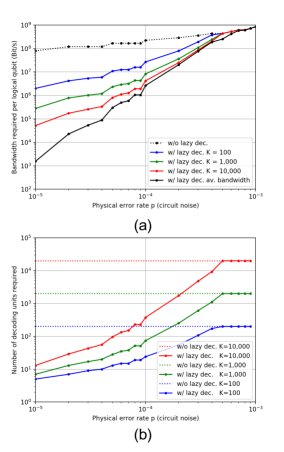
Figure 5: (a) Bandwidth required per logical qubit in Bit/s for different number of logical qubits $K$ to reach a target logical error rate of $10^{-15}$. (b) Number of decoding units required for a system of $K$ logical qubits in order to reach a target logical error rate of $10^{-15}$.

Fig. 5 shows the bandwidth required to reach a target logical error rate $p_{\operatorname{target}}=10^{-15}$. Given $p_{\operatorname{target}}$ and the physical error rate $p$ of the device, we first pick the smallest minimum distance $d$ that ensures $p_{L}(p,d)<p_{\operatorname{target}}$ using Eq. 1. The minimum distance varies discretely with $p$, inducing brutal jumps in the system requirements. Once the distance is fixed, we estimate the lazy decoder failure probability $p_{\bf fail}(p,d)$ by a Monte-Carlo simulation, from which we derive the value of $\operatorname{bw}_{\operatorname{lazy}}(p,d,K)$ based on Eq. (4). A better distribution of resources is achieved for a system that contains many logical qubits, dropping the bandwidth required per logical qubits closer to the average use. The bandwidth saturation appears again in the regime $p=10^{-3}$ where we require almost 1GBits/s per logical qubit. For error rates $p\geq 6.10^{-4}$, we observe no saving for bandwidth requirements.

V Decoding hardware requirements

In addition to a substantial bandwidth reduction, the lazy decoder induces savings in the decoding hardware. Indeed, the value $M(p,d,K)$ introduced in Eq. (4) is the largest number of decoding tasks to perform simultaneously over the whole system of $K$ logical qubits. Instead of allocating one decoding unit for each logical qubit, one can share $M(p,d,K)$ decoding units without notably affecting the failure rate of the quantum computer. Fig. 5, shows the saving in term of number of decoding units. In order to reach a target error rate of $10^{-15}$ with a system of $K=10,000$ logical qubits with physical error rate $p=10^{-4}$ (resp. $10^{-5}$) a naive design uses $2K=20,000$ decoding units while only 377 units (resp. 13) are sufficient with the lazy decoder, saving $98\%$ (resp. $99.9\%$) of the decoding hardware. Table 1 shows the saving and the hardware requirements for different target noise rate, qubit quality and system size. Again, the saturation in the regime $p=10^{-3}$ limits the saving. We need better qubits in order to scale up quantum computers to the massive size required for practical applications.

Table 1: Decoding Hardware Requirements with Lazy Decoder for different system sizes. We indicate the fraction of decoding hardware saved by the Lazy decoder.

$p_{target}=10^{-15}$
$p$	$K=100$	$K=1,000$	$K=10,000$
	$d=29$	$d=29$	$d=29$
$10^{-3}$	84 GBit/s	840 GBit/s	8.4 TBit/s
	200 dec. units	2,000 dec. units	20,000 dec. units
	save $0\%$	save $0\%$	save $0\%$
	$d=15$	$d=15$	$d=15$
$10^{-4}$	2,7 GBit/s	8,3 GBit/s	42 GBit/s
	24 dec. units	74 dec. units	377 dec. units
	save $88\%$	save $96\%$	save $98\%$
	$d=9$	$d=9$	$d=9$
$10^{-5}$	200 MBit/s	280 MBit/s	520 MBit/s
	5 dec. units	7 dec. units	13 dec. units
	save $97.5\%$	save $99.7\%$	save $99.9\%$
$p_{target}=10^{-12}$
$p$	$K=100$	$K=1,000$	$K=10,000$
	$d=23$	$d=23$	$d=23$
$10^{-3}$	53 GBit/s	530 GBit/s	5.3 TBit/s
	200 dec. units	2,000 dec. units	20,000 dec. units
	save $0\%$	save $0\%$	save $0\%$
	$d=11$	$d=11$	$d=11$
$10^{-4}$	900 MBit/s	2,4 GBit/s	10.5 GBit/s
	15 dec. units	40 dec. units	175 dec. units
	save $93\%$	save $98\%$	save $99\%$
	$d=7$	$d=7$	$d=7$
$10^{-5}$	96 MBit/s	144 MBit/s	216 MBit/s
	4 dec. units	6 dec. units	9 dec. units
	save $98\%$	save $99.7\%$	save $99.96\%$
$p_{target}=10^{-9}$
$p$	$K=100$	$K=1,000$	$K=10,000$
	$d=17$	$d=17$	$d=17$
$10^{-3}$	29 GBit/s	290 GBit/s	2.9 TBit/s
	200 dec. units	2,000 dec. units	20,000 dec. units
	save $0\%$	save $0\%$	save $0\%$
	$d=7$	$d=7$	$d=7$
$10^{-4}$	168 MBit/s	360 MBit/s	1.2 GBit/s
	7 dec. units	15 dec. units	51 dec. units
	save $97\%$	save $99.3\%$	save $99.8\%$
	$d=5$	$d=5$	$d=5$
$10^{-5}$	24 MBit/s	36 MBit/s	60 MBit/s
	2 dec. units	3 dec. units	5 dec. units
	save $99\%$	save $99.9\%$	save $99.98\%$

VI The lazy decoder as a decoder accelerator

The lazy decoder can be considered as a (hardware or software) decoder accelerator. It speeds up any decoding algorithm without significantly degrading the correction capability. Fig. 6 shows the average execution time for our implementation in C of two standard decoding algorithms with and without lazy pre-decoding. The speed-up reaches a factor 10x for the Union-Find (UF) decoder Delfosse and Nickerson (2017), which is already one of the fastest decoding algorithms and we obtain a 50x acceleration of the Minimum Weight Perfect Matching (MWPM) decoder Dennis et al. (2002). Note that both combinations Lazy + UF and Lazy + MWPM achieve a similar average runtime, although the worst-case execution time, which is a central parameter in the design of a decoding architecture Das et al. (2020), is substantially larger for the MWPM.

We also confirmed numerically that the lazy decoder does not deteriorate the performance of the MWPM decoder and the UF decoder as Theorem 1 suggests. On the contrary, the lazy decoder provides a slight improvement of the correction capacity of the UF decoder. This is because these two algorithms perform well on different types of fault configurations. The work of Seth et al. Sheth et al. (2019b) explores further the idea of combining different decoding strategies.

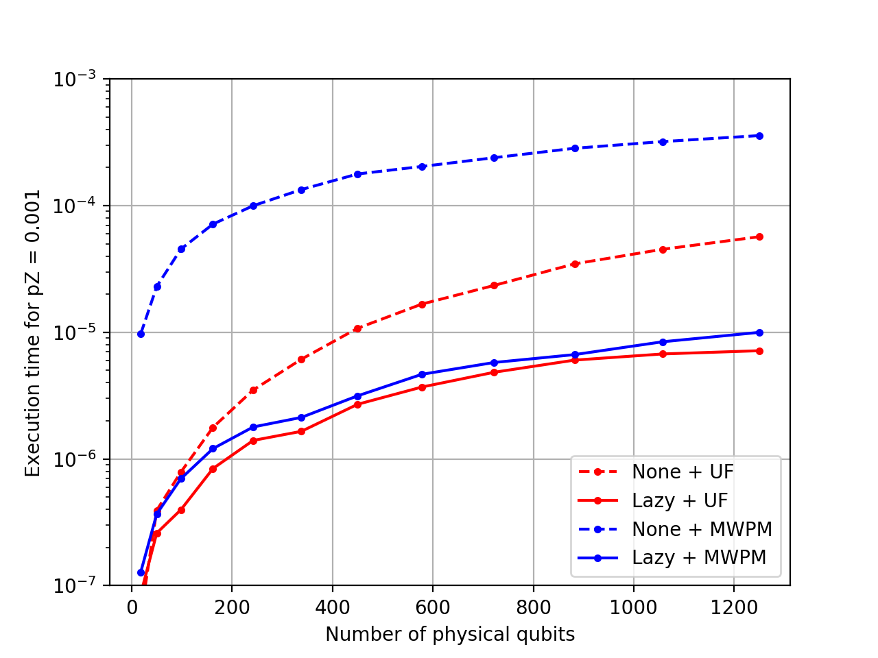
Figure 6: Execution time in seconds of the MWPM decoder and the UF decoder with and without lazy decoder. The runtime is estimated over $10^{6}$ trials, over the 2D toric code, assuming perfect measurements and an error rate of $10^{-3}$. We use an implementation in C of these algorithms executed on a MacBook Pro 2013 with a single thread processor 2,4 GHz Intel Core i5. We observe a 10x speed-up of the UF decoder and 50x for the MWPM decoder.

Conclusion – Error correction is a major bottleneck in fault-tolerant quantum computing which leads to a huge overhead in the implementation of quantum algorithms Reiher et al. (2017); Campbell et al. (2019); Gidney and Ekerå (2019). In this article, we designed a simple decoder that can be used in combination with a more complex decoding unit to correct errors simultaneously on many logical qubits with a minimum decoding hardware.

In future work, we plan to explore the impact of serialization latency on the decoder’s performance.

Although this work focuses on surface codes, the general principle of this design can be adapted to any quantum error correction code if we can identify a set of easy error configuration that is likely enough.

The lazy decoder applies to any type of surface code, including codes defined on non-trivial topology Zémor (2009); Breuckmann et al. (2017). The lazy decoder can be directly applied to color codes Bombin and Martin-Delgado (2006) using for instance the projection decoder Delfosse (2014); Kubica and Delfosse (2019).

Beyond topological codes, one can adapt the lazy decoder to quantum LDPC codes MacKay et al. (2004); Tillich and Zémor (2013); Gottesman (2014); Fawzi et al. (2018); Campbell (2019); Breuckmann and Londe (2020). The sparsity of the Tanner graph guarantees the success of our local strategy for low enough physical error rate.

The basic idea of using a pre-decoder dedicated to the correction of simple configurations is also central in the design of a flash memory controller where a hard-decision belief propagation (BP) decoder is used as a pre-decoder and, in case of failure, multiple levels of soft-decision BP are performed Cai et al. (2017). However, the noise rate of flash cells is far more favorable than in quantum hardware, allowing for using a single decoding unit to correct many encoded blocks in flash memory. Note that the execution time current flash BP decoders are far too long for the quantum setting if we suppose that the decoding must be implemented in $d\mu s$. ($80\mu s$ for hard decision decoder + $80\mu s$ per level of soft-BP) Cai et al. (2017).

The BP decoder provides a hierarchy of decoding algorithms with growing complexity as a function of the number of propagation levels. This flexibility allows for adjusting the number of levels in order to maximize the success probability of the decoder according the decoding available time. The Union-Find decoder Delfosse and Nickerson (2017) offers the same advantage by tuning the number of growth rounds.

In the future, it would be interesting to explore further the hardware implementation of the Lazy decoder following the approach of Das et al. (2020) and to fabricate an FPGA or ASIC prototype in order to obtain a better insight on practical applications of the lazy decoder.

Acknowledgement – The author would like to thank Krysta Svore, Michael Beverland, Jeongwan Haah, Adam Paetznick, Chris Pattison, Poulami Das, Alan Geller, Matthias Troyer, Helmut Katzgraber and Dave Wecker for insightful discussions and Poulami Das for her comments on a preliminary version of this article.

References

- Dennis et al. (2002) E. Dennis, A. Kitaev, A. Landahl, and J. Preskill, Journal of Mathematical Physics 43, 4452 (2002).
- Fowler et al. (2012a) A. G. Fowler, M. Mariantoni, J. M. Martinis, and A. N. Cleland, Physical Review A 86, 032324 (2012a).
- Raussendorf and Harrington (2007) R. Raussendorf and J. Harrington, Physical Review Letters 98, 190504 (2007).
- Fowler et al. (2009) A. G. Fowler, A. M. Stephens, and P. Groszkowski, Physical Review A 80, 052312 (2009).
- Gidney and Ekerå (2019) C. Gidney and M. Ekerå, arXiv preprint arXiv:1905.09749 (2019).
- Fowler et al. (2012b) A. G. Fowler, A. C. Whiteside, A. L. McInnes, and A. Rabbani, Physical Review X 2, 041003 (2012b).
- Fowler et al. (2012c) A. G. Fowler, A. C. Whiteside, and L. C. Hollenberg, Physical review letters 108, 180501 (2012c).
- Fowler (2015) A. G. Fowler, Quantum Information and Computation 15, 0145 (2015).
- Duclos-Cianci and Poulin (2010) G. Duclos-Cianci and D. Poulin, Physical review letters 104, 050504 (2010).
- Duclos-Cianci and Poulin (2013) G. Duclos-Cianci and D. Poulin, arXiv preprint arXiv:1304.6100 (2013).
- Barrett and Stace (2010) S. D. Barrett and T. M. Stace, Physical review letters 105, 200502 (2010).
- Stace and Barrett (2010) T. M. Stace and S. D. Barrett, Physical Review A 81, 022317 (2010).
- Delfosse and Zémor (2017) N. Delfosse and G. Zémor, arXiv preprint arXiv:1703.01517 (2017).
- Fowler (2013) A. G. Fowler, arXiv preprint arXiv:1310.0863 (2013).
- Delfosse and Tillich (2014) N. Delfosse and J.-P. Tillich, in 2014 IEEE International Symposium on Information Theory (IEEE, 2014), pp. 1071–1075.
- Criger and Ashraf (2018) B. Criger and I. Ashraf, Quantum 2, 102 (2018).
- Nickerson and Brown (2019) N. H. Nickerson and B. J. Brown, Quantum 3, 131 (2019).
- Dennis (2005) E. Dennis, arXiv preprint quant-ph/0503169 (2005).
- Harrington (2004) J. W. Harrington, Ph.D. thesis, California Institute of Technology (2004).
- Wootton and Loss (2012) J. R. Wootton and D. Loss, Physical review letters 109, 160503 (2012).
- Hutter et al. (2014) A. Hutter, J. R. Wootton, and D. Loss, Physical Review A 89, 022326 (2014).
- Wootton (2015) J. Wootton, Entropy 17, 1946 (2015).
- Herold et al. (2015) M. Herold, M. J. Kastoryano, E. T. Campbell, and J. Eisert, arXiv preprint arXiv:1511.05579 (2015).
- Breuckmann et al. (2016) N. P. Breuckmann, K. Duivenvoorden, D. Michels, and B. M. Terhal, arXiv preprint arXiv:1609.00510 (2016).
- Delfosse and Nickerson (2017) N. Delfosse and N. H. Nickerson, arXiv preprint arXiv:1709.06218 (2017).
- Tomita and Svore (2014) Y. Tomita and K. M. Svore, Physical Review A 90, 062320 (2014).
- Heim et al. (2016) B. Heim, K. M. Svore, and M. B. Hastings, arXiv preprint arXiv:1609.06373 (2016).
- Torlai and Melko (2017) G. Torlai and R. G. Melko, Physical review letters 119, 030501 (2017).
- Baireuther et al. (2018) P. Baireuther, T. E. O’Brien, B. Tarasinski, and C. W. Beenakker, Quantum 2, 48 (2018).
- Krastanov and Jiang (2017) S. Krastanov and L. Jiang, Scientific reports 7, 11003 (2017).
- Varsamopoulos et al. (2017) S. Varsamopoulos, B. Criger, and K. Bertels, Quantum Science and Technology 3, 015004 (2017).
- Chamberland and Ronagh (2018) C. Chamberland and P. Ronagh, Quantum Science and Technology 3, 044002 (2018).
- Breuckmann and Ni (2018) N. P. Breuckmann and X. Ni, Quantum 2, 68 (2018).
- Sweke et al. (2018) R. Sweke, M. S. Kesselring, E. P. van Nieuwenburg, and J. Eisert, arXiv preprint arXiv:1810.07207 (2018).
- Baireuther et al. (2019) P. Baireuther, M. Caio, B. Criger, C. W. Beenakker, and T. E. O’Brien, New Journal of Physics 21, 013003 (2019).
- Ni (2018) X. Ni, arXiv preprint arXiv:1809.06640 (2018).
- Andreasson et al. (2019) P. Andreasson, J. Johansson, S. Liljestrand, and M. Granath, Quantum 3, 183 (2019).
- Davaasuren et al. (2018) A. Davaasuren, Y. Suzuki, K. Fujii, and M. Koashi, arXiv preprint arXiv:1801.04377 (2018).
- Liu and Poulin (2019) Y.-H. Liu and D. Poulin, Physical review letters 122, 200501 (2019).
- Varsamopoulos et al. (2018) S. Varsamopoulos, K. Bertels, and C. G. Almudever, arXiv preprint arXiv:1811.12456 (2018).
- Varsamopoulos et al. (2019) S. Varsamopoulos, K. Bertels, and C. G. Almudever, arXiv preprint arXiv:1901.10847 (2019).
- Wagner et al. (2019) T. Wagner, H. Kampermann, and D. Bruß, arXiv preprint arXiv:1910.01662 (2019).
- Chinni et al. (2019) C. Chinni, A. Kulkarni, and D. M. Pai, arXiv preprint arXiv:1901.07535 (2019).
- Sheth et al. (2019a) M. Sheth, S. Z. Jafarzadeh, and V. Gheorghiu, arXiv preprint arXiv:1905.02345 (2019a).
- Colomer et al. (2019) L. D. Colomer, M. Skotiniotis, and R. Muñoz-Tapia, arXiv preprint arXiv:1911.02308 (2019).
- Ferris and Poulin (2014) A. J. Ferris and D. Poulin, Physical review letters 113, 030501 (2014).
- Bravyi et al. (2014) S. Bravyi, M. Suchara, and A. Vargo, Physical Review A 90, 032326 (2014).
- Darmawan and Poulin (2018) A. S. Darmawan and D. Poulin, Physical Review E 97, 051302 (2018).
- Tuckett et al. (2018) D. K. Tuckett, C. T. Chubb, S. Bravyi, S. D. Bartlett, and S. T. Flammia, arXiv preprint arXiv:1812.08186 (2018).
- Das et al. (2020) P. Das, C. A. Pattison, S. Manne, D. Carmean, K. Svore, M. Qureshi, and N. Delfosse, arXiv preprint arXiv:2001.06598 (2020).
- Sheth et al. (2019b) M. Sheth, S. Z. Jafarzadeh, and V. Gheorghiu, arXiv preprint arXiv:1905.02345 (2019b).
- Zémor (2009) G. Zémor, in International Conference on Coding and Cryptology (Springer, 2009), pp. 259–273.
- Breuckmann et al. (2017) N. P. Breuckmann, C. Vuillot, E. Campbell, A. Krishna, and B. M. Terhal, Quantum Science and Technology 2, 035007 (2017).
- Bombin and Martin-Delgado (2006) H. Bombin and M. A. Martin-Delgado, Physical review letters 97, 180501 (2006).
- Delfosse (2014) N. Delfosse, Physical Review A 89, 012317 (2014).
- Kubica and Delfosse (2019) A. Kubica and N. Delfosse, arXiv preprint arXiv:1905.07393 (2019).
- MacKay et al. (2004) D. J. C. MacKay, G. Mitchison, and P. L. McFadden, IEEE Transaction on Information Theory 50, 2315 (2004).
- Tillich and Zémor (2013) J.-P. Tillich and G. Zémor, IEEE Transactions on Information Theory 60, 1193 (2013).
- Gottesman (2014) D. Gottesman, Quantum Information & Computation 14, 1338 (2014).
- Fawzi et al. (2018) O. Fawzi, A. Grospellier, and A. Leverrier, in 2018 IEEE 59th Annual Symposium on Foundations of Computer Science (FOCS) (IEEE, 2018), pp. 743–754.
- Campbell (2019) E. Campbell, Quantum Science and Technology (2019).
- Breuckmann and Londe (2020) N. P. Breuckmann and V. Londe, arXiv preprint arXiv:2001.03568 (2020).
- Cai et al. (2017) Y. Cai, S. Ghose, E. F. Haratsch, Y. Luo, and O. Mutlu, arXiv preprint arXiv:1711.11427 (2017).
- Reiher et al. (2017) M. Reiher, N. Wiebe, K. M. Svore, D. Wecker, and M. Troyer, Proceedings of the National Academy of Sciences 114, 7555 (2017).
- Campbell et al. (2019) E. Campbell, A. Khurana, and A. Montanaro, Quantum 3, 167 (2019).