Kelly Betting with Quantum Payoff: a continuous variable approach
Abstract
The main purpose of this study is to introduce a semi-classical model describing betting scenarios in which, at variance with conventional approaches, the payoff of the gambler is encoded into the internal degrees of freedom of a quantum memory element. In our scheme, we assume that the invested capital is explicitly associated with the quantum analog of the free-energy (i.e. ergotropy functional by Allahverdyan, Balian, and Nieuwenhuizen) of a single mode of the electromagnetic radiation which, depending on the outcome of the betting, experiences attenuation or amplification processes which model losses and winning events. The resulting stochastic evolution of the quantum memory resembles the dynamics of random lasing which we characterize within the theoretical setting of Bosonic Gaussian channels. As in the classical Kelly Criterion for optimal betting, we define the asymptotic doubling rate of the model and identify the optimal gambling strategy for fixed odds and probabilities of winning. The performance of the model are hence studied as a function of the input capital state under the assumption that the latter belongs to the set of Gaussian density matrices (i.e. displaced, squeezed thermal Gibbs states) revealing that the best option for the gambler is to devote all their initial resources into coherent state amplitude.
1 Introduction
The problem of assessing the maximum growth of an optimal investment, or equivalently of the maximization of the long-run interest rate, is one of the central issues in quantitative finance. An especially simple but fundamental example is provided by horse-race markets, i.e. markets with the property that at every time step one of the assets pays off and all the other assets pay nothing (the wealth invested is lost completely). Remarkably, horse-race markets are very special cases of general markets, being, in a sense, the extremal points of the distribution of asset returns [1, 2]. As such they have been extensively investigated: they possess many of the usual attributes of financial markets but they also have the important additional property that each bet has a well defined end point at which its value becomes certain. This is rarely the case in finance, where asset values depend on an intrinsically uncertain future [3]. In the 1950s, J. L. Kelly, Jr. worked out a striking interpretation of the rate of transmission of information over a noisy communication channel in the setting of gambling theory [4].
In this context, the input symbols to the communication line were interpreted as the outcomes of an uncertain event on which betting is possible.
Exploiting this construction, under “fair" odds and independent and identically distributed (i.i.d.) horse-race markets assumptions (with no transactions costs), Kelly proved the optimality of
proportional betting strategies; specifically, he proved that the asymptotic growth rate of the cumulative wealth is maximal when the fraction of capital bet on each horse is proportional to its true winning probability. Remarkably, over the years, both theory and practice of the Kelly criterion in gambling and investment have developed prolifically [5].
In this paper, we present a theory of classical betting with a quantum payoff which investigates the behaviour of an economic agent whose initial capital is represented by the value of a quantum resource encoded into the state of a quantum memory that faces uncertainty under action of a stochastic environment.
In order to achieve this, we rely on the versatility of Bosonic Gaussian channels (BGCs) to mimic the action of the random gains and losses that affect the capital in a horse-race market.
BGCs play a fundamental role in quantum information theory
[6, 7]
where they act as the proper counterparts of Gaussian channels of classical information theory
(see, for instance [8, 9, 10]and references therein). Formally speaking, they can be identified
with the set of quantum evolutions which preserve the “Gaussian character" of the transmitted signals and possess the striking feature, heavily used in this paper, to be closed under composition [11]. At the physical level BGCs describe the most relevant transformations an optical pulse may experience when
propagating in a noisy environment. In particular, they provide a proper
representation of attenuation and amplification processes for continuous variable quantum systems [8, 10]. Differently from their classical counterparts, which can be always realized without extra added noise effects,
BGCs include vacuum fluctuation and display a non-commutative character
which has an intrinsic quantum mechanical origin. As a result, the setting we introduce here is inherently different from previously analyzed horse-market models [3, 12], giving rise to a non-trivial generalization of classical betting procedures.
The connection between game theory and quantum information has a long history dating back to the pioneering results presented in
Refs. [13, 14, 15].
The common denominator of these works is to grant players access to quantum resources
like entanglement or mere quantum coherence,
that help them in defining new strategies, thus enlarging the range of possible operations.
Our approach on the contrary relies on quantizing not the protocol itself but only the resource that is used to encode both the invested capital and the payoff of the game. Specifically,
in our model we identify the capital of our economic agent with the quantum ergotropy functional [16] associated to the density matrix of a single Bosonic mode that is under the control of the
agent. Ergotropy plays an important role in many different contexts, spanning from the characterization of optimal thermodynamical cycles [17, 18]
to energetic instabilities [19, 20], and to the study of quantum batteries models [16, 21, 22]: it
represents the maximum mean energy decrement obtainable when forcing the quantum system to undergo unitary evolutions induced by cyclic external modulations of its Hamiltonian. The use of the ergotropy as a quantifier of the wealth of the agent is legitimated by the fact that in the Kelvin-Planck formulation of the second law of thermodynamics,
can be interpreted as the maximum amount of useful energy (work) which we can extract form the state
via reversible coherent (i.e. unitary) transformations, i.e, in the absence of extra resources and without collateral dissipation events [23].
This choice follows also the long history of analogy making between economics (and finance) and (stastical)
thermodynamics discussed for instance in [24, 25, 26], and references therein. It is worth observing also that our representation of the invested capital reminds somehow the proposal of Orrell which used the energy (not the ergotropy) of an harmonic oscillator to describe the price of transactions occurring during a trading cycle [27, 28].
Regarding the uncertainty of the outcome of the horse race, we describe it with the random selection of one among a collection of a finite set of one-mode BGCs operating on . Their action includes both an attenuation part – associated with the partition of the capital determined by the strategy adopted by the gambler – and an amplification part –associated instead with the odds offered by the bookmaker. Each channel is therefore randomly selected and applied to according to the winning probability of the corresponding horse. The whole procedure is iterated to reproduce the i.i.d. horse-race markets framework, resulting into a stochastic
trajectory for in which the state of the system at the discrete time step , is obtained by a concatenation of elements of the selected BGCs set.
We notice that from a practical standpoint our construction is a simple idealization of a general random lasing process [29], so the formalism we introduce here could also serve as a modelization
of the thermodynamic aspects of light amplification in disordered materials.
The resulting payoff for the gambler is therefore computed by evaluating the ergotropy functional
on the final state of the problem. The aim of our work is characterizing the probability distribution of the resulting accumulated wealth and determining which, among all possible choices of the input state of , provides the best performance in terms of capital-gain for a given game strategy. It is worth stressing that at the level of the mere internal energy of the system , irrespective of the choice of the initial state , the process (3.16) behaves essentially as its classical horse-market counterpart, a part from a noisy contribution, where the BGCs are replaced by standard betting operations. On the contrary, at the level of ergotropy, the non-commutative nature of the involved quantum operation, combined with the classical randomness of the bet, results in the injection of extra noise terms which affect negatively the performance of the procedure, paving the way for a nontrivial optimization of the initial resource . In our analysis we shall address this problem by explicitly restricting the class of allowed inputs to the special (yet not trivial) subset of Gaussian density matrices [11]. This choice on one hand allows for some mathematical simplification while on the other hand
is physically motivated by the fact that this special collection of states includes a rather large class of electromagnetic configurations (notably thermal, coherent, and squeezed signals)
that are very well under experimental control.
The rest of the paper is organized as follows: we start in Sec. 2 with a brief review on BGCs. The Kelly model with quantum payoff is hence introduced in Sec. 3. In Sec. 4 we study its statistical properties and present
some numerical analysis. Conclusions are presented in Sec. 5.
The manuscript also contains an Appendix devoted to elucidate some technical aspects of the problem.
2 Preliminaries
2.1 Gaussian states
Let be a complex separable Hilbert space of infinite dimension associated with one mode of the electromagnetic radiation (or equivalently a 1-dimensional, quantum harmonic oscillator) of frequency . The model is fully described by the assignment of the canonical coordinate vector and the quadratic Hamiltonian
| (2.1) |
expressed in terms of (rescaled) position and momentum operators and which satisfy the (Bosonic) canonical commutation relation: ( being the Planck constant). We let be the set of the positive semidefinite operators with trace , and we call a quantum state of if . For each element of such set we can then associate a column vector of ,
| (2.2) |
given by the expectation values of the canonical coordinates, and a covariance matrix whose elements are
| (2.3) |
with denoting the anti-commutator operation, which describes instead the second order moments of the coordinate distributions on . Although no constraints hold on , on quantum uncertainty relations impose the inequality , with being the second Pauli matrix. An exhaustive description of is finally provided by the characteristic function formalism which, given a density matrix allows us to faithfully represents it in terms of the following complex functional
| (2.4) |
where is a column vector of , and is the Weyl operator of the system. In this context, the density matrix is thus said to be Gaussian if its associated characteristic function has a Gaussian form, i.e. namely if we have
| (2.5) |
with and defined as in Eqs. (2.2) and (2.3) respectively [11]. At the physical level Gaussian states represent thermal Gibbs density matrices of generic Hamiltonians which are (non-negative) quadratic forms of the canonical vector . A convenient parametrization is given by the following expression
| (2.6) |
where for , defines a thermal state of the mode Hamiltonian (2.1) with inverse temperature ( being the associated partition function) and where for complex we introduce the squeezing operator
| (2.7) |
with being a rotation matrix defined in terms of the first and third Pauli matrices and . With this choice we get that the associated characteristic function of (2.6) is in the form (2.5) with
| (2.8) | |||||
where is the identity matrix and is the average photon number of . Special cases of Gaussian states are the coherent states which often are referred to as semi-classical configurations of the electro-magnetic field obtained by setting in (2.6).
2.2 One-mode Bosonic Gaussian channels
A BGC is a Completely Positive, Trace Preserving (CPTP) dynamical transformation [6, 7] defined by assigning a column vector of , and two positive real matrices and fulfilling the constraint
| (2.9) |
When operating on a generic , sends it into a new density matrix whose characteristic function is expressed by the formula
| (2.10) |
At the level of first and second moments, this mapping induces the transformation
| (2.11) |
the couple , being associated with the input state , and , being instead associated with the output state . These transformations inherit their name from the notable fact that when applied to an arbitrary Gaussian input they will produce Gaussian outputs. Most importantly for us, these processes are closed under super-operator composition, meaning that given two BGC maps and identified respectively by the triples and , the transformation obtained by concatenating them in sequence is still a BGC channel characterized by the new triple
| (2.12) |
As already mentioned in the introduction, at physical level BGCs describe a vast variety of processes. In what follows we shall focus on the special subset of BGCs associated with amplification and attenuation events, possibly accompanied by thermalization effects. These maps have and , proportional to . In view of the constraint (2.9) and following a rather standard convention, we find it useful to express them in terms of two non-negative constants as , with
| (2.15) |
and use the notation to represent the associated channel. Notice that in this case Eq. (2.11) gets simplified as
| (2.16) | |||||
| (2.17) |
which allows us to interpret as a stretching parameter for the first moments of the state, and as an additive noise term. Furthermore from (2.12) it trivially follows that the BGC subset formed by the maps is also closed under channel composition leading to the following identity
| (2.18) |
with
| (2.19) |
For , defines a process where the mode interacts dispersively with an external thermal Bosonic envinronment characterized by a mean photon number (thermal attenuator channel). In particular for and (i.e. ) we get
| (2.20) |
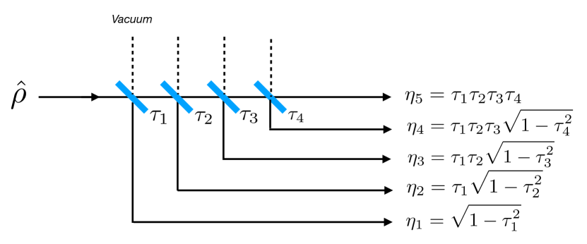
which describes a pure loss of energy from the system, corresponding to the evolution the mode experiences when passing through a medium (beam-splitter) of transmissivity . A special case of particular interest for us is depicted in Fig. 1 where a collection of beam-splitters (semitransparent mirrors [30]) are arranged to split an input optical signal into a different direction by properly mixing it with the vacuum. In this construction, while the joint state emerging from the set up may exhibit nontrivial correlations, the local density matrices associated to the various output ports are described as with being the corresponding effective transmissivity.
For , describes instead the interaction of and the thermal bath in terms of an amplification event (thermal amplifier). In this case for and (i.e. ) the transformation
| (2.21) |
defines a purely amplifying process induced by the interaction between and the vacuum mediated by a non-linear optical crystal [30]. Finally, we observe that in the special case where , the transformation
| (2.22) |
corresponds to the noise-additive channel which describes a random Gaussian displacement in the phase space [8].
2.3 Average energy and ergotropy
The mean energy of a generic state of the mode is given by
| (2.23) |
where is the square norm of , where in the second identity we made explicit use of Eqs. (2.2) and (2.3), and where without loss of generality we set . For a Gaussian state, exploiting the parametrization introduced in Eq. (2.6), this can be cast in a formula that highlights the squeezing, displacement, and thermal contributions to the final result, i.e.
| (2.24) |
Equations (2.23) and (2.24) represent the total energy stored in which one could extract from the , e.g. by putting it in thermal contact with an external zero-temperature environment. Yet, as pointed out in Ref. [31, 32], not all such energy will be nicely converted into useful work: part of will indeed necessarily emerge as dissipated heat. The quantity that instead properly quantifies the maximum amount of extractable work is given by the ergotropy. At variance with , the latter is a nonlinear functional of that we can compute as
| (2.25) |
where the minimization is performed over all unitary transformations . For a one-mode Bosonic Gaussian state a closed expression in terms of and is known which we shall use in the following, i.e. [22]
| (2.26) | |||||
This equation shows that the gap between and only depends upon the thermal component of , i.e.
| (2.27) |
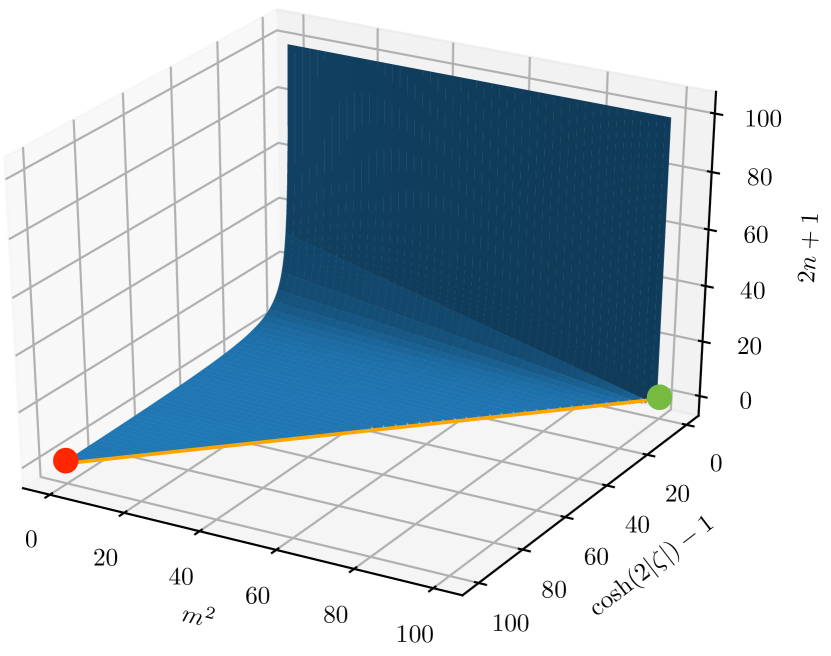
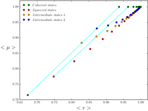
reaching its minimum value for pure (squeezed coherent) states (i.e. ) where it matches the vacuum energy level . Notice also that states which are characterized by the same ergotropy value form a continuous 2D manifold in the phase space associated with the variables , , and – see Fig. 2.
3 The playing field
Motivated by the Kelly Criterion for optimal betting and the versatility of the one-mode BGCs, we present here a theory of classical betting with a quantum payoff. First, in Subsection 3.1 we briefly review the conventional Kelly setting. Then in Subsection 3.2, we introduce the repeated-quantum-betting scheme as the iteration of single quantum bets, each bet being a probabilistic transmission of the quantum state of a single Bosonic mode through a one-mode BGC. We hence embed the protocol into a rigorous mathematical framework. Not only this allows for a more compact representation of the procedure over time, but also it enables to see the iterative scheme from the higher perspective of random dynamical systems: the action of a family of quantum transformations, corresponding to one-mode BGCs in the procedure, over a phase space of (single Bosonic mode) quantum states. Finally in Subsection 4 we construct a parallel between the quantum and the classical Kelly criterion.
3.1 The Kelly Criterion for optimal betting
Imagine that one has horses competing in a race, each characterized by a winning probability , . Formally speaking the ’s define a distribution of a random variable taking values in the alphabet with probability (symbols of the alphabet representing the horses whereas the variable the winning horse). If a gambler invests one dollar on horse then they receive dollars if horse wins and zero dollars if horse loses: the game is then said to be under unfair odds condition if ; on the contrary, if or we say that the odds are fair or super-fair respectively. In what follows we shall always focus on these last two cases for which one can show that the best gaming option for the gambler is always to distribute all of their wealth across the horses (constant allocation strategy). Accordingly we call the fraction of the gambler’s wealth invested in horse , and . We consider henceforth a sequence of repeated gambles on this race under i.i.d. assumptions, i.e. requiring that neither the probabilities s, the odds s, and the fractions s vary from betting stage to betting stage. The wealth of the gambler during such a sequence is a random variable defined by the expression
| (3.1) |
where for , represents the horse that has won the -th race delivering a payoff , the corresponding joint probability being
| (3.2) |
(to help readability hereafter we adopt the compact convention of dropping explicit reference of the functional dependence upon the indexes , , , of quantities evaluated along a given stochastic trajectory). In the asymptotic limit of large , the value of can be directly linked to the doubling rate of the horse race, i.e. the quantity
| (3.3) |
where , and are the three vectors which, under i.i.d. assumptions fully define the model: the first assigning the stochastic character of the race, the second the selected odds of the broker, and the last one the strategy the gambler adopts in placing his bets. More specifically, the connection between and is provided by the strong Law of Large Numbers (LLN) which in the present case establishes that for sufficiently large we have almost surely, or more precisely that
| (3.4) |
see for instance [33], Theorem 6.6.1. Exploiting this result, one can now identify the optimal gambling strategy that ensures the largest asymptotic wealth increase, by selecting which allows to reach its maximum value for fixed and . Such maximum is achieved by the proportional gambling scheme where (Kelly criterion) so that
| (3.5) |
with the Shannon entropy of the Bernoulli distribution defined by the vector (see [33], Theorem 6.1.2).
3.2 BGC betting model
As in the previous section we consider a horse-race model where at each step of the gambling scheme horses compete, their probability of winning being defined by a Bernoulli distribution . At variance with the typical Kelly setting we assume that the capital the gambler invests in the game is represented not by conventional money, but instead by the ergotropy (2.25) they store into a single Bosonic mode initially prepared into the density matrix which, as anticipated in the introduction, is assumed to belong to the Gaussian subset.
To place their bet, at each race the gambler divides his capital exploiting an optical splitter analogous to one shown in Fig. 1 which distributes the input mode into independent outputs characterized by effective transmissivities , each associated with an individual horse and fulfilling the normalization condition
| (3.6) |
This implies that the capital the gambler is placing on the horse is locally stored into the density matrix obtained by applying the purely lossy BGC mapping of Eq. (2.20) to the entry capital of the betting stage. The parameters clearly reflect the gambler game strategy and play the role of the fractions of the original Kelly’s model (more precisely, due to constraint (3.6) the exact correspondence is between the s and the squares of the network transmissivities). In case the -th horse wins, the corresponding output port will hence undergo a coherent amplification event which pumps up the energy level of the system via the gain parameter and is returned to the gambler, the other sub-modes being instead absorbed away. At the level of this results in a transformation described by the pure amplifier BGC mapping introduced in Eq. (2.21). The parameters reflect the odds parameters of the classical model. Again the exact correspondence is between the s and the squares of the amplification amplitudes which allows us to translate the fair odds and super-fair odds conditions into the requirements
| (3.7) | |||||
| (3.8) |
respectively, which we shall assume hereafter.
In summary, after each betting stage the gambler receives back the state of their single mode resource quantum memory, transformed via the combined action of a purely lossy map and a pure amplifier, i.e. the BGC map which according to (2.18) can be written as
| (3.9) |
where now, for all , the stretching and noise terms are given by
| (3.10) | |||||
| (3.11) |
The composition property (2.18) also lends itself well to the framework of repeated gambles described in Sec. 3.1.
Specifically, assuming the initial state of to be described by the density matrix , after the fist betting event, with probability , the gambler will get the state
| (3.12) |
which they will use to place the second bet (notice that following the same convention introduced in the previous section, the functional dependence of upon the index is left implicit). Accordingly, with conditional probability the second horse race will induce the following mapping on
| (3.13) |
At the level of input density matrix , Eq. (3.13) corresponds to the stochastic mapping
| (3.14) |
where
| (3.15) |
is the composite BGC map obtained by merging together and and occurs with joint probability . More generally, indicating with the state of after steps along a given stochastic realization of the horse race described by a winning string of event , the transformation (3.13) gets replaced by the mapping
| (3.16) |
which occurs with probability . Similarly the transformation (3.14) becomes
| (3.17) |
where now the -fold mapping is given by
| (3.18) |
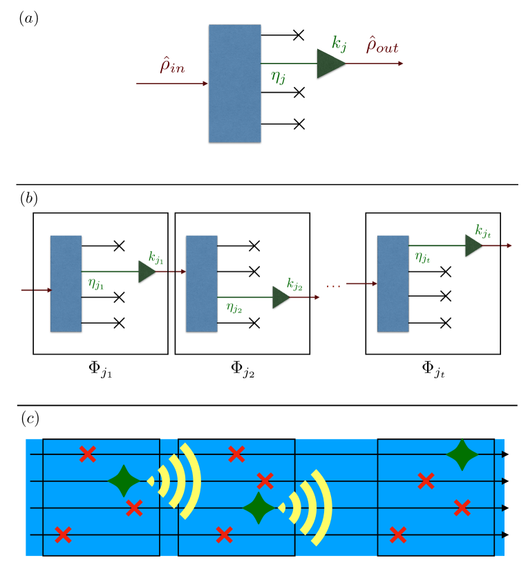
and occurs with joint probability defined as in Eq. (3.2) – the whole process being visualized in Fig. 3. We notice that from Eq. (3.9) and the general composition rule (2.18) it follows that
| (3.19) |
where the parameter is given by
| (3.20) |
while is defined by the recursive formula
| (3.24) |
which, as shown in Lemma 1 of the Appendix, admits the following solution
| (3.25) |
Before proceeding any further it is worth stressing that the map defined above describes the state of after steps along a given trajectory of the betting process. Taking the weighted mean of these super-operators with probabilities gives instead the transformation which defines the evolution of the system irrespective of the history of the betting process. Explicitly this is given by
| (3.26) |
with the CPTP map defined by the convex convolution
| (3.27) |
which does not necessarily correspond to a BGC. It is finally worth stressing that the scheme provides an effective, lumped-element model description of propagation of light modes inside a multi-layer material where, depending on the layer, they get randomly amplified (as in a stimulated emission process) or attenuated (as in an absorption process), the stochastic channel describing the system evolution conditioned to the realization of a specific history of events – see panel (c) of Fig. 3. As a matter of fact our setting provides an effective model for random lasing [29]. A random laser is a device where coherent light amplification is achieved without the presence of an optical cavity, through a sequence of stochastic events that may occur in disordered materials [34, 35] due to multiple-scattering effects [36, 37]. At the level of the the electromagnetic radiation, such processes will lead to trajectories which ultimately can be characterized as multi-mode versions of the maps introduced in Eq. (3.18), with the channels describing the gains and losses experienced by the signal in their random walk through the active media.
3.3 Quantum payoff of the BGC model
From the above results it is now easy to express the energy associated with the state of at a generic step along a given trajectory. Indeed from (2.16) and (2.17) it follows that the first order expectation vector and the covariance matrix of can be written as
| (3.28) | |||||
| (3.29) |
where and are their corresponding counterparts associated with the input state . Therefore, the mean energy of the system is now given by
| (3.30) |
where we introduced the quantity
| (3.31) |
and where is the mean energy of the input state. Parametrizing the latter as in (2.24), Eq. (3.30) can then be casted in the form
| (3.32) |
Similarly, reminding that is a Gaussian state, from Eqs. (2.27), (3.28), and (3.29), we can express the ergotropy of as
| (3.33) |
with being the thermal contribution to the total photon number of the final state computed as
| (3.34) |
In our construction Eq. (3.33) represents the payoff of the gambler after steps. By re-organizing the various contributions, it can be conveniently casted into the form
| (3.35) |
where
| (3.36) |
is the initial value of the ergotropy, i.e. the initial capital invested by the player. In the above expression
| (3.37) |
is a non-negative quantity which, while not being directly linked to , is an explicit functional of the selected input state (here ). This fact has profound consequences as it implies that, differently from the original Kelly’s scheme, in our setting the final payoff is not just proportional to the initial invested capital , but also depends in a nontrivial way on the type of input state that was selected to "carry" the value of such capital. Accordingly in discussing the performance of the betting scheme we are now facing an extra layer of optimization where the gambler, beside selecting the transmissivities and deciding the value of they want to invest in the game, has also the possibility of deciding which one of the input states that belongs to the same iso-ergotropy manifold (see of Fig. 2) they want to adopt: different choices will indeed result in different and hence in different payoff values .
3.4 Input state optimization
Let start observing that from Eq. (3.35) it follows that if the input state of the system is a purely Gibbs thermal state of the system Hamiltonian (i.e. if ) then the capital gain is strictly null at all time steps, i.e. for all : this implies that in order to have at a chance of getting some positive payoff, the player needs to invest at least a non-zero capital (a very reasonable contraint). Notice also that if we restrict to a semiclassical case in which is described by a noisy coherent state (i.e. for ), we get and hence
| (3.38) |
implying that under this assumption the capital evolves as the classical case of a geometric game. Departures from Eq. (3.38) can instead be observed when squeezing is present in the initial state of the system paving the way to the optimization problem mentioned at the end of the previous paragraph, i.e. deciding what is the best choice of to be employed in the betting scheme for assigned values of and .
To tackle this issue we find it useful to define two different figures of merit, i.e. the renormalized ergotropy functional which, as gauges the absolute payoff, and the output ergotropy ratio , aimed instead to characterize the amount of resources wasted in the process. The first quantity is simply obtained by rescaling the payoff capital by the term in order to contrast the potential divergent behaviour of the former, i.e.
| (3.39) |
For fixed choices of and , exhibits the same dependence upon upon the input state , with the main advantage of being bounded from above by 1 (on the contrary, as we already mentioned, can explode). The second quantity instead is defined as the ratio between the ergotropy and the mean energy of the state , i.e.
where
| (3.41) |
is the value of the ratio computed on the input state . Notice that by construction and are bounded quantities that cannot exceed the value 1. Furthermore irrespective of the parameters of the model and from the outcome of the stochastic process, cannot be larger than its initial value : indeed an upper bound for can be obtained by setting equal to zero the squeezing parameter of the initial state (i.e. ) which leads to
| (3.42) |
the rightmost inequality following as a consequence of the positivity of . Equation (3.42) implies that, even though the gambler has a chance of increasing its wealth (i.e the value of the ergotropy of the mode ), in the quantum model we are considering here this always occurs at the cost of an inevitable waste of resources.
It goes without mentioning that, as in the case of the payoff capital , the figures of merit introduced above are stochastic quantities which strongly depend on the random sequence of betting events. Interestingly enough however a mere analysis of the functional dependence of , upon the input data of the problem, allows us to draw some important conclusions even without carrying out a full statistical analysis of the process (a task which, as we shall see in the next section, is rather complex). For this purpose we first notice that from Eq. (3.38) it follows that setting , i.e. using input states which have no squeezing, is the proper choice to bust to its upper bound 1. This choice also ensures the saturation of the first inequality in Eq. (3.42), leading us to an output ergotropy ratio that expressed in terms of can be written as
| (3.43) |
the last inequality being saturated by setting . Accordingly we can conclude that, for fixed values of and game strategy , the best choice for the input density matrix is the pure coherent input state of the selected iso-ergotropy manifold (i.e. the green dot of Fig. 2) since, irrespective of the specific outcomes of the stochastic process that drives the system dynamics, this will ensure the saturation of the functional upper bounds for both the two figures of merit we have introduced. The above inequalities show the optimality of coherent input states for any and . At each step the resulting concatenation of BGCs results in a noisy attenuation/amplification map, so the gambler cannot gain more ergotropy by using a different strategy even with an adaptive one.
4 Statistical analysis
In Kelly’s language each bet in our gambling problem is identified with the drawing of a Bernoulli random variable and the overall gain/loss of each bet is identified with the parameters and . In particular, in the new playing field, the analogoue of the gambler’s wealth after races, of Sec. 3.1, is the quantity of Eq. (3.33). As discussed in the previous section the latter is computed through the action of the BGC of Eq. (3.19) which determines the evolution of the quantum mode via Eq. (3.17) and which is fully characterized by the parameters and . As anticipated in Eq. (3.38), in the absence of input squeezing (i.e. ) the first of these two quantities, i.e. , represents the amplification of the input signal in the model, the gambler’s wealth being directly proportional to . The presence of squeezing in the initial state, makes the connection between and the payoff more complex (see Eq. (3.33)) still a direct comparison between Eq. (3.20) and (3.1) makes it explicit that shares the same statistical properties of the function of the classical setting. In particular also in this case we can use the strong LLN to replace Eq. (3.4) with
| (4.1) |
where now
| (4.2) |
substitute the doubling rate of Eq. (3.3) – here , and . Accordingly we can claim that almost surely for sufficiently large. Furthermore simple algebra allows one to show that the optimal energy splitting strategy which yields the maximum doubling rate
| (4.3) |
which is obtained by setting
| (4.4) |
which represents precisely the Kelly criterion for the optimal choice of the betting strategy.
Let us now turn our attention to the second stochastic quantity which defines the model, i.e. the parameter . This term measures the noise generated in the process due to the random application of quantum BGC, and it appears thanks to the non-commutative nature of our quantum model. From a close inspection of Eq. (3.24) we observe that is generated by the iteration of a family of random Lipschitz maps[38], precisely affine random maps with random slope and random intercept. For instance in the case where the total number of horses in the race is with , , this can be made explicit by starting with and writing with
| (4.5) |
Depending on the value of we can distinguish different scenarios. The one that is best characterized at the mathematical level is when the model is contracting on average [39], i.e. when , which unfortunately is the less interesting case for our model as it represents a betting scheme where the player asymptotically looses all its capital. Under this condition there exists a unique stationary invariant probability measure for the process which can be singular or absolutely continuous [40]. For instance, referring to the parametrization introduced in Eq. (4.5), when in the case if then, up to an affine map, the invariant measure of the system is a Bernoulli convolution [41]. These measures have been studied since the 1930’s, revealing connections with harmonic analysis, the theory of algebraic numbers, dynamical systems and fractal geometry. It is well-known that in some cases they are singular (more precisely when the inverse of the contraction rate is an especially "symmetric" type of irrational algebraic number, a so-called Pisot number [42]). When instead, the measure is the Lebesgue measure whereas if it is the uniform measure on a Cantor set (i.e. a totally disconnected closed subset of the real line consisting entirely of boundary points). Such sets may have zero or positive Lebesgue measure. They are typically fractal sets and the uniform measure is equivalent to the the Hausdorff measure of dimension equal to the dimension of the Cantor set (see [43] for more details). Generally speaking in the contractive-on-average case the fundamental fact which one can exploit is that the random family of maps contracts the Wasserstein metric on compactly supported probability measures. If this assumption is not met then the situation is considerably more complex: orbits can be dense on the real half-line [44] and one can investigate to what extent their distribution is uniform [45].
The situation becomes even more problematic in the case which is more interesting for us, i.e. for maps that are expanding-on-average, i.e. when . Not much attention has been devoted to the study of this scenario: as a matter of fact, the only reference we could find[46] investigates only the orbits of the associated topological dynamical systems obtained by suitably renormalizing the –th iterates. We contribute to the effort by noticing that in these cases due to the fact that is almost surely a divergent quantity (see e.g. (4.1)), it is convenient to focus on the renormalized version of introduced in Eq. (3.31), which determines the stochastic evolution of indicators and defined in Sec. 3. It turns out that is rather regular and for finite , its first and second moments can be computed (see Lemma 2 of the Appendix). Furthermore it is possible to show that the random parameter converges almost surely whenever diverges exponentially almost surely: this is a consequence of the fact that is -th partial sum of the infinite series with -th term that always exists due to the non-negativity of the terms, and it is guaranteed to be finite when the denominator can be upper bounded by an exponentially diverging term, as it gives a trivial upper bound by a convergent geometric series (see the Theorem 1 of the Appendix for a more detailed derivation of this result). We also observe that, since both and are positive quantities bounded from above, it makes sense to determine the asymptotic values and as the (point-wise) limit of the distribution for :
| (4.6) |
Despite this nice property, determining the effective distribution of and (or those of and for finite), remains however a rather complex task and at present we are not able to make general claims. To compensate for this, we do however present a numerical analysis that allows us to at least get some insights on the problem.
4.1 Numerics
In this section we simulate numerically the evolution of and over a sufficiently long time horizon to infer their asymptotic behaviour. In Figs. 7–5 the temporal evolution of the empirical distributions of these quantities have been reconstructed by sampling simulations for each temporal step and for various choices of the parameters and in the two-horse case (i.e. ). In the plots we also report the temporal evolutions of the average values of and extracted from the sampling. It goes without mentioning that due to the nonlinear dependence of these functionals upon the state of the system, they do not coincide with the corresponding values computed on the average density matrix of the system obtained by applying the average map (3.26) to . In all the figures we also exhibit an educated guess for the average value of obtained by naively replacing the terms that appears in Eq. (3.4) with its average value computed as in the Appendix. This quantity can be thought of as a mean field approximation of our random variable and it is written as
| (4.7) |
with
| (4.8) |
converging to the asymptotic value .
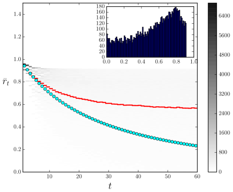
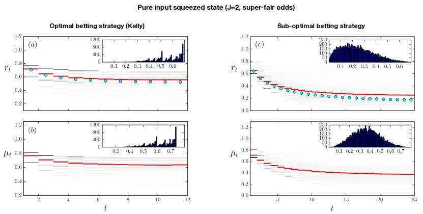
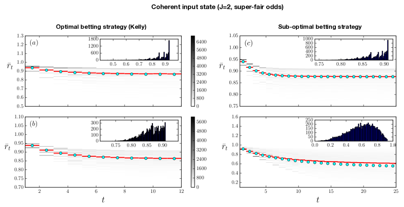
Let us now enter into the details of our numerical analysis. In Fig. 7, focusing on the same betting scenario, we compare the results obtained when adopting the optimal (Kelly) betting strategy (4.4) (panels (a) and (b)) with those of a sub-optimal one (panels (c) and (d)), for a pure squeezed input state, under super-fair odds conditions. As clear from the plots the Kelly strategy leads to a beneficial increment both in terms of the mean values of and (attaining higher values in the (a) and (b) panels), as well as in terms of their spreads (more concentrated toward higher values in the (a) and (b) panels). Similar findings are confirmed in Fig. 8 were instead we focus on the case of a pure coherent state (in this case we only present , since one always get for all due to Eq. (3.38)). A direct comparison between the panels (a) of the Figs. 7 and 8, also show that under the same betting conditions, and input ergotropy resources, the coherent inputs provide better performances than pure squeezed states in agreement with the results of Sec. 3.4. This fact is also confirmed by the data of Fig. 6 which present a numerical estimation of the asymptotic averaged values of and of Eq. (4.6) for various choices of pure (displaced-squeezed) input state while maintaining the same (optimal) betting strategy. The detrimental influence of thermal photons in the input state is instead addressed in Fig. 4 where the temporal distribution of is studied under optimal betting strategies and the same game conditions discussed in the panels (a) of Figs. 7 and 8: despite exhibiting the same input ergotropy one notices that the range and the mean value exhibited by get contracted with respect to both the coherent and squeezed case.
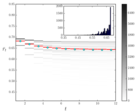
As a general remark we point out that the shape that we observe for the asymptotic distributions of and are a direct consequence of the underlying binomial process which generates a random walk on with steps whose length and direction at time depend on the position at time [47]. We highlight also that when choosing as the optimal Kelly-betting strategy (4.4) and to be a vector of super-fair odds (3.8), then we have finiteness of the first moment of – see panels (a) and (b) of Figs. 7–6. The same stability condition has been enforced also for all the other configurations we have considered, apart from the case reported in Fig. 5: here choosing as the optimal Kelly-betting strategy (4.4) and setting to be a vector of fair odds (3.7), while all the moments of remain finite (because it has support contained in the interval ), one has (see Lemma (2) in appendix) which tends to compromise the convergency of the simulations as evident from the reported data and the matching with the mean field estimation (4.7).
5 Conclusions and future perspectives
Betting (or gambling) is a practical tool for studying decision-making in face of classical uncertainty. The optimal betting strategy has been in the mathematical literature since the 1950s. Known as the classical Kelly criterion for optimal betting, it holds that under “fair" odds and i.i.d. repeated horse-races you should bet a fraction of capital on each horse that is proportional to the true winning probabilities of the latter in order to maximize the asymptotic growth rate of the cumulative wealth.
In this paper, we presented a semi-classical model describing betting scenarios where the payoff of the gambler is encoded into the internal degrees of freedom of a quantum memory element. We provided a translation of the classical Kelly framework into the new semi-classical playing field. Specifically, the invested capital was associated with the ergotropy of a single mode of the electromagnetic radiation; the losses and winning events with the attenuation and amplification processes of the just-mentioned single-mode; instead, the (random) evolution of the capital, represented by the evolution of the quantum memory, is characterized within the theoretical setting of Bosonic Gaussian channels. As in the classical Kelly Criterion for optimal betting, we defined the asymptotic doubling rate of the model and identified the optimal gambling strategy for fixed odds and winning probabilities. We carried out an accurate statistical and numerical analysis to determine the performance of the model.
We found that if the input capital state belongs to the set of Gaussian density matrices then the best option for the gambler is to devote all their initial resources into coherent state amplitude.
A first natural problem to address is the generalization of our constructions to multimode scenarios. This would pave the way for
the study of non-classical interference effects in betting games where the gambler can distribute their capital on parallel independent horse-races. In particular, this happens quite often in reality [3, 5] and the comparison across different racetrack markets is fundamental in analysing their informational efficiency. Moreover, since the late nineties, platforms allowing short as well as long bets have been introduced (betting exchanges). This allows bettors to wager against over-priced horses just as hedge fund managers can short financial contracts. Finding an adequate quantum setting for betting exchanges, including possibly general financial markets, would considerably extend the
set of applications of our framework.
Finally an interesting perspective is also offered by the possibility of employing the random
CPT trajectory model introduced in Sec. 3.2 to analyse the lasing effects in random materials [29].
The Authors would like to thank Giuseppe La Rocca for insightful discussions regarding the possible applications of the formalism to study random lasing events. V. G. acknowledges support by MIUR via PRIN 2017 (Progetto di Ricerca di Interesse Nazionale): project QUSHIP (2017SRNBRK).
The authors acknowledge the financial support of UniCredit Bank RD group through the Dynamics and Information Research Institute at the Scuola Normale Superiore.
References
- Bell and Cover [1988] R. Bell and T. M. Cover. Game-theoretic optimal portfolios. Management Science, 34(6):724–733, 1988. doi: 10.1287/mnsc.34.6.724.
- Iyengar and Cover [2000] G. N. Iyengar and T. M. Cover. Growth optimal investment in horse race markets with costs. IEEE Transactions on Information Theory, 46(7):2675–2683, 2000. doi: 10.1109/18.887881.
- Williams [2005] L. V. Williams. Information efficiency in financial and betting markets. Cambridge University Press, 2005. doi: 10.1017/CBO9780511493614.
- Kelly [1956] J. L. Kelly. A new interpretation of information rate. The Bell System Technical Journal, 35(4):917–926, 1956. doi: 10.1002/j.1538-7305.1956.tb03809.x.
- MacLean et al. [2011] L. C. MacLean, E. O. Thorp, and W. T. Ziemba. The Kelly capital growth investment criterion: Theory and practice, volume 3. World Scientific, 2011. doi: 10.1142/7598.
- Holevo [2012] A. S. Holevo. Quantum Systems, Channels, Information: A Mathematical Introduction. De Gruyter, 2012. doi: 10.1515/9783110273403.
- Wilde [2017] M. M. Wilde. Quantum Information Theory. Cambridge University Press, 2 edition, 2017. doi: 10.1017/9781316809976.
- Holevo and Werner [2001] A. S. Holevo and R. F. Werner. Evaluating capacities of bosonic gaussian channels. Physical Review A, 6(032312), 2001. doi: 10.1103/PhysRevA.63.032312.
- Caruso et al. [2006] F. Caruso, V. Giovannetti, and A. S. Holevo. One-mode bosonic gaussian channels: a full weak-degradability classification. New Journal of Physics, 8(12):310, 2006. doi: 10.1088/1367-2630/8/12/310.
- Giovannetti et al. [2014] V. Giovannetti, R. García-Patrón, N. J. Cerf, and A. S. Holevo. Ultimate classical communication rates of quantum optical channels. Nature Photonics, 8:796–800, 2014. doi: 10.1038/nphoton.2014.216.
- Serafini [2017] A. Serafini. Quantum Continuous Variables. CRC Press, 2017. doi: 10.1201/9781315118727.
- Hausch et al. [2008] D. B. Hausch, V. S. Lo, and W. T. Ziemba. Efficiency of racetrack betting markets, volume 2. World Scientific, 2008. doi: 10.1142/6910.
- Meyer [1999] D. A. Meyer. Quantum strategies. Physical Review Letters, 82(5):1052, 1999. doi: 10.1103/PhysRevLett.82.1052.
- Goldenberg et al. [1999] L. Goldenberg, L. Vaidman, and S. Wiesner. Quantum gambling. Physical Review Letters, 82(16):3356, 1999. doi: 10.1103/PhysRevLett.82.3356.
- Eisert et al. [1999] J. Eisert, M. Wilkens, and M. Lewenstein. Quantum games and quantum strategies. Physical Review Letters, 83(15):3077, 1999. doi: 10.1103/PhysRevLett.83.3077.
- Alicki and Fannes [2013] R. Alicki and M. Fannes. Entanglement boost for extractable work from ensembles of quantum batteries. Physical Review E, 87(042123), 2013. doi: 10.1103/PhysRevE.87.042123.
- Alicki and Kosloff [2018] R. Alicki and R. Kosloff. Introduction to Quantum Thermodynamics: History and Prospects, pages 1–33. Springer International Publishing, 2018. doi: 10.1007/978-3-319-99046-0_1.
- Bera et al. [2018] M. N. Bera, A. Winter, and M. Lewenstein. Thermodynamics from information, pages 799–820. Springer International Publishing, 2018. doi: 10.1007/978-3-319-99046-0_33.
- Pusz and Woronowicz [1978] W. Pusz and S. L. Woronowicz. Passive states and kms states for general quantum systems. Communications in Mathematical Physics, 58(3):273–290, 1978. doi: 10.1007/BF01614224.
- Lenard [1978] A. Lenard. Thermodynamical proof of the gibbs formula for elementary quantum systems. Journal of Statistical Physics, 19(6):575–586, 1978. doi: 10.1007/BF01011769.
- Andolina et al. [2019] G. M. Andolina, M. Keck, A. Mari, M. Campisi, V. Giovannetti, and M. Polini. Extractable work, the role of correlations, and asymptotic freedom in quantum batteries. Physical Review Letters, 122(047702), 2019. doi: 10.1103/PhysRevLett.122.047702.
- Farina et al. [2019] D. Farina, G. M. Andolina, A. Mari, M. Polini, and V. Giovannetti. Charger-mediated energy transfer for quantum batteries: An open-system approach. Physical Review B, 99(035421), 2019. doi: 10.1103/PhysRevB.99.035421.
- Niedenzu et al. [2019] W. Niedenzu, M. Huber, and E. Boukobza. Concepts of work in autonomous quantum heat engines. Quantum, 3:195, October 2019. doi: 10.22331/q-2019-10-14-195.
- Smith and Foley [2008] E. Smith and D. K. Foley. Classical thermodynamics and economic general equilibrium theory. Journal of economic dynamics and control, 32(1):7–65, 2008. doi: 10.1016/j.jedc.2007.01.020.
- Kim and Marmi [2015] D. H. Kim and S. Marmi. Distribution of asset price movement and market potential. Journal of Statistical Mechanics: Theory and Experiment, 2015(7):P07001, 2015. doi: 10.1088/1742-5468/2015/07/P07001.
- Saslow [1999] W. M. Saslow. An economic analogy to thermodynamics. American Journal of Physics, 67(12):1239–1247, 1999. doi: 10.1119/1.19110.
- Orrell [2020a] D. Orrell. A quantum model of supply and demand. Physica A: Statistical Mechanics and its Applications, 539:122928, 2020a. ISSN 0378-4371. doi: 10.1016/j.physa.2019.122928.
- Orrell [2020b] D. Orrell. The value of value: A quantum approach to economics, security and international relations. Security Dialogue, 51(5):482–498, 2020b. doi: 10.1177/0967010620901910.
- Wiersma [2008] D. S. Wiersma. The physics and applications of random lasers. Nature Physics, 4(5):359–367, May 2008. doi: 10.1038/nphys971.
- Walls and Milburn [2008] D. F. Walls and G. J. Milburn. Quantum Optics. Springer-Verlag, 2008. doi: 10.1007/978-3-540-28574-8.
- Allahverdyan et al. [2004] A. E. Allahverdyan, R. Balian, and Th. M. Nieuwenhuizen. Maximal work extraction from finite quantum systems. Europhysics Letters, 67(4):565, 2004. doi: 10.1209/epl/i2004-10101-2.
- Brown et al. [2016] E. G. Brown, N. Friis, and M. Huber. Passivity and practical work extraction using gaussian operations. New Journal of Physics, 18, 2016. doi: 10.1088/1367-2630/18/11/113028.
- Cover and Thomas [2012] T. M. Cover and J. A. Thomas. Elements of Information Theory. John Wiley & Sons, 2012. doi: 10.1002/047174882X.
- Markushev et al. [1986] V. M. Markushev, V. F. Zolin, and Ch. M. Briskina. Powder laser. Zhurnal Prikladnoi Spektroskopii, 45:847–850, 1986.
- Lawandy et al. [1994] N. M. Lawandy, R. M. Balachandran, A. S. L. Gomes, and E. Sauvain. Laser action in strongly scattering media. Nature, 368(6470):436–438, March 1994. doi: 10.1038/368436a0.
- Letokhov [1968] V.S. Letokhov. Generation of light by a scattering medium with negative resonance absorption. Soviet Physics JETP, 26(4):835, April 1968. URL https://ui.adsabs.harvard.edu/abs/1968JETP...26..835L/abstract.
- Wiersma and Lagendijk [1996] D. S. Wiersma and A. Lagendijk. Light diffusion with gain and random lasers. Physical Review E, 54:4256–4265, October 1996. doi: 10.1103/PhysRevE.54.4256.
- Bhattacharya and Majumdar [2007] R. Bhattacharya and M. Majumdar. Random dynamical systems: theory and applications. Cambridge University Press, 2007. doi: 10.1017/CBO9780511618628.
- Nicol et al. [2002] M. Nicol, N. Sidorov, and D. Broomhead. On the fine structure of stationary measures in systems which contract-on-average. Journal of Theoretical Probability, 15(3):715–730, 2002. doi: 10.1023/A:1016224000145.
- Diaconis and Freedman [1999] P. Diaconis and D. Freedman. Iterated random functions. SIAM review, 41(1):45–76, 1999. doi: 10.1137/S0036144598338446.
- Gouezel [2019] S. Gouezel. Méthodes entropiques pour les convolutions de bernoulli (d’après hochman, shmerkin, breuillard, varju). Asterisque, (414):251–287, 2019. doi: 10.24033/ast.1086.
- Bertin et al. [1992] M. J. Bertin, A. Decomps-Guilloux, M. Grandet-Hugot, M. Pathiaux-Delefosse, and J. Schreiber. Pisot and Salem Numbers. Birkhäuser Basel, 1992. doi: 10.1007/978-3-0348-8632-1.
- Falconer [2003] K. Falconer. Fractal Geometry: Mathematical Foundations and Applications. John Wiley & Sons, Ltd, 2 edition, 2003. doi: 10.1002/0470013850.
- Misiurewicz and Rodrigues [2005] M. Misiurewicz and A. Rodrigues. Real . Proceedings of the American Mathematical Society, 133(4):1109–1118, 2005. doi: 10.1090/S0002-9939-04-07696-8.
- Bergelson et al. [2006] V. Bergelson, M. Misiuriewicz, and S. Senti. Affine actions of a free semigroup on the real line. Ergodic Theory and Dynamical Systems, 26(5):1285–1305, 2006. doi: 10.1017/S014338570600037X.
- Demichel [2018] Y. Demichel. Renormalization of the hutchinson operator. SIGMA. Symmetry, Integrability and Geometry: Methods and Applications, 14:085, 2018. doi: 10.3842/SIGMA.2018.085.
- Evertsz and Mandelbrot [1992] C. J. G. Evertsz and B. B. Mandelbrot. Multifractal measures, volume 1092, pages 921–953. Springer-Verlag, New York, 1992. doi: 10.1007/978-1-4757-4740-9.
Lemma 1 (Recurrence relation for ).
The recurrence relation (3.24) admits the solution
| (.1) |
Proof.
The parameters and define the action of the BGC (3.19). By the equation (3.24) we have:
| (.2) |
Now using as defined in (3.20), we can find an explicit formula for :
So we can solve for , integrating the finite difference:
| (.3) |
since we have that we obtain:
| (.4) |
and recalling the definition 3.31 of we obtain the thesis. ∎
We conclude this part by deriving some properties of .
Lemma 2 (Moments of ).
If we call
then
| (.5) |
and
| (.6) |
Proof.
The expected value of is:
where we used the fact that the different bets are independent.
Regarding the second moment of , we split it into two terms as:
where the second term can also be written as:
| (.9) | |||||
∎
Corollary 1.
Under the assumptions that and it results that:
| (.10) |
Proof.
By definition is a positive and monotonically increasing sequence, so for the monotone convergence theorem we have that:
If we take the limit of the formulas in lemma (2) we obtain the thesis ∎
Theorem 1.
If diverges exponentially almost surely then converges almost surely.
Proof.
We just need to prove that the sequence is a Cauchy sequence almost everywhere in our probability space. To formally embed the statement in a rigorous mathematical framework, we should introduce a probability space where the Bernoulli distribution on , and to be the -algebra generated by the cylinder sets. Then taking we identify with the define quantity (3.20 ) computed on the first elements of , and define . In this language Eq. (4.1) formally translates into
| (.11) |
where is a short hand notation for . Accordingly given
| (.12) |
it follows that
| (.13) |
Now, let . Fix , and let as in Eq.(.12). Then for all
| (.14) |
Let , with . For a chosen
| (.15) | |||||
for some constants – we are using the convention of indicating with the quantity (3.31) associated with the first elements of . For a sufficiently large we have . Hence we proved that
or equivalently that is a Cauchy sequence almost everywhere. ∎