Prospects of tensor-based numerical modeling of the collective electrostatic potential in many-particle systems

Abstract

Recently the rank-structured tensor approach suggested a progress in the numerical treatment of the long-range electrostatic potentials in many-particle systems and the respective interaction energy and forces [39, 40, 2]. In this paper, we outline the prospects for tensor-based numerical modeling of the collective electrostatic potential on lattices and in many-particle systems of general type. We generalize the approach initially introduced for the rank-structured grid-based calculation of the collective potentials on 3D lattices [39] to the case of many-particle systems with variable charges placed on $L^{\otimes d}$ lattices and discretized on fine $n^{\otimes d}$ Cartesian grids for arbitrary dimension $d$. As result, the interaction potential is represented in a parametric low-rank canonical format in $O(dLn)$ complexity. The energy is then calculated in $O(dL)$ operations. Electrostatics in large biomolecules is modeled by using the novel range-separated (RS) tensor format [2], which maintains the long-range part of the 3D collective potential of the many-body system represented on $n\times n\times n$ grid in a parametric low-rank form in $O(n)$-complexity. We show that the force field can be easily recovered by using the already precomputed electric field in the low-rank RS format. The RS tensor representation of the discretized Dirac delta [45] enables the construction of the efficient energy preserving (conservative) regularization scheme for solving the 3D elliptic partial differential equations with strongly singular right-hand side arising, in particular, in bio-sciences. We conclude that the rank-structured tensor-based approximation techniques provide the promising numerical tools for applications to many-body dynamics, protein docking and classification problems, for low-parametric interpolation of scattered data in data science, as well as in machine learning in many dimensions.

Key words: Coulomb potential, Slater potential, long-range many-particle interactions, low-rank tensor decomposition, range-separated tensor formats, summation of electrostatic potentials, energy and force calculations.

AMS Subject Classification: 65F30, 65F50, 65N35, 65F10

1 Introduction

Numerical modeling of electrostatics in the large ensembles of charged particles is considered since long as a challenging problem. Computation of the electrostatic interactions in many-body dielectric systems like solute-solvent complexes is a complicated numerical problem in molecular dynamics simulations of large solvated biological systems, in docking or folding of proteins, pattern recognition, the assembly of polymer particles in colloidal physics and many other problems [31, 35, 8, 34, 36, 56, 57, 55]. Most numerical schemes for modeling these problems are based either on use of FEM/FDM discretization or on application of integral formulations for solving the arising PDEs. On the other hand, the complicated many-particle interaction processes are often modeled by using the stochastic Monte Carlo approaches, avoiding the traditional deterministic methods of high computational complexity.

Tensor-structured numerical methods are now becoming popular in scientific computing due to their intrinsic property of reducing the grid-based solution of multidimensional problems in $\mathbb{R}^{d}$ to basically “one-dimensional” computations. These methods evolved from bridging of the traditional rank-structured tensor formats in multilinear algebra [14, 12, 10, 69, 26, 24] with the nonlinear approximation theory based on a separable representation of multivariate functions and operators [27, 22, 42]. One of the important ingredients of tensor decomposition methods in multilinear algebra was the so-called higher order SVD (HOSVD) introduced for the rank reduction in the Tucker tensors [15] and further extended to the TT tensor format [62, 23, 60]. Development of tensor techniques for numerical solution of multidimensional problems in scientific computing was promoted by the reduced HOSVD (RHOSVD) method introduced in [47]. It allows to reduce the tensor rank in the canonical format by the canonical-to-Tucker (C2T) decomposition without the need to construct the full size tensor. The RHOSVD was initially used for the rank reduction in canonical tensors in calculation of three-dimensional convolution integrals in computational quantum chemistry, see [44, 41] and the references therein.

In this paper, we outline the beneficial features of the tensor-based numerical modeling of long-range interactions in many-particle systems, which allows to avoid the exponential complexity scaling in dimension, that is typical for the traditional numerical approaches. In the recent decade there was a burst of new results on rank-structured tensor approximation of radial-type multivariate functions arising in computer simulations of many-particle ensembles [39, 40, 2, 51]. In what follows, we generalize the tensor-based approach introduced in [39, 40] which allows to represent the collective electrostatic potential of a complex lattice-type system on an $n\times n\times n$ 3D Cartesian grid in a parametric canonical or Tucker-type formats by using a small number of terms leading to $O(n)$ complexity. We discuss how electrostatics in bio-molecular complexes can be modeled by using the RS tensor format, which maintains the long-range part of the 3D charge distribution and the collective potential in a low-parametric rank-structured form in $O(n)$-complexity [2, 45, 3]. The RS tensor decomposition can be applied to wide classes of radial functions providing the low-rank representation of long-range part in large sums of the corresponding generating kernels. In this paper we present the RS decomposition for the Slater function and provide the comparative analysis with the RS splitting of the Newton kernel. We show how the RS tensor representation of the free-space potential and electric field allows to calculate energy and forces for many-particle systems in low cost.

The rest of the paper is structured as follows. Section 2 presents a short overview of classical approaches for numerical modeling of the long-range interaction potentials. Section 2.1 recalls the construction of the canonical tensor representation of the Newton kernel, which was the base for further developments. Section 2.2 discusses the direct tensor summation of Newton kernels in the nuclear potentials, which yet does not maintain the full power of tensor-based modeling. Section 3.2 presents the new results on assembled tensor summation of the interaction potentials of charged particles centered at nodes of a 3D lattice, yielding the linear complexity scaling for energy calculation in the univariate lattice size. Section 4 describes the main ideas and advantages of the recent RS tensor format in numerical modeling of electrostatics in many-body systems of general type. Section 5 discusses the application of RS tensor format in bio-molecular modeling including the energy and force calculations. Section 7 sketches the main rank-structured tensor formats.

2 Canonical tensor approximation of interaction potentials

2.1 Low-rank canonical representation of radial functions

First, we recall the grid-based method for the low-rank canonical representation of a spherically symmetric kernel function $p(\|x\|)$, $x\in\mathbb{R}^{d}$ for $d=2,3,\ldots$, by its projection onto the finite set of basis functions defined on tensor grid. The approximation theory by a sum of Gaussians for the class of analytic potentials $p(\|x\|)$ was presented in [70, 27, 22, 42, 44]. The particular numerical schemes for rank-structured representation of the Newton and Yukawa Green’s kernels

$$p(\|x\|)=\frac{1}{4\pi\|x\|},\quad\mbox{ and }\quad p(\|x\|)=\frac{e^{-\lambda\|x\|}}{4\pi\|x\|},\quad x\in\mathbb{R}^{3},$$ (2.1)

discretized on a fine 3D Cartesian grid in the form of low-rank canonical tensor was described in [27, 42, 5].

In what follows, for the ease of exposition, we confine ourselves to the case $d=3$. In the computational domain $\Omega=[-b,b]^{3}$, let us introduce the uniform $n\times n\times n$ rectangular Cartesian grid $\Omega_{n}$ with mesh size $h=2b/n$ ($n$ even). Let $\{\psi_{\textbf{i}}=\prod_{\ell=1}^{3}\psi_{i_{\ell}}^{(\ell)}(x_{\ell})\}$ be a set of tensor-product piecewise constant basis functions, labeled by the $3$-tuple index ${\bf i}=(i_{1},i_{2},i_{3})$, $i_{\ell}\in I_{\ell}=\{1,...,n\}$, $\ell=1,\,2,\,3$. The generating kernel $p(\|x\|)$ is discretized by its projection onto the basis set $\{\psi_{\textbf{i}}\}$ in the form of a third order tensor of size $n\times n\times n$, defined entry-wise as

$$\mathbf{P}:=[p_{\bf i}]\in\mathbb{R}^{n\times n\times n},\quad p_{\bf i}=\int_{\mathbb{R}^{3}}\psi_{\bf i}({x})p(\|{x}\|)\,\,\mathrm{d}{x}.$$ (2.2)

The low-rank canonical decomposition of the $3$rd order tensor $\mathbf{P}$ is based on using exponentially convergent $\operatorname*{sinc}$-quadratures for approximating the Laplace-Gauss transform to the analytic function $p(z)$, $z\in\mathbb{C}$, specified by a certain weight $\widehat{p}(t)>0$,

$$p(z)=\int_{\mathbb{R}_{+}}\widehat{p}(t)e^{-t^{2}z^{2}}\,\mathrm{d}t\approx\sum_{k=-M}^{M}p_{k}e^{-t_{k}^{2}z^{2}}\quad\mbox{for}\quad|z|>0,\quad z\in\mathbb{R},$$ (2.3)

with the proper choice of the quadrature points $t_{k}$ and weights $p_{k}$. The $sinc$-quadrature based approximation to generating function by using the short-term Gaussian sums in (2.3) are applicable to the class of analytic functions in certain strip $|z|\leq D$ in the complex plane, such that on the real axis these functions decay polynomially or exponentially. We refer to basic results in [70, 7, 27], where the exponential convergence of the $sinc$-approximation in the number of terms (i.e., the canonical rank) was analyzed for certain classes of analytic integrands.

Now, for any fixed $x=(x_{1},x_{2},x_{3})\in\mathbb{R}^{3}$, such that $\|{x}\|>a>0$, we apply the $\operatorname*{sinc}$-quadrature approximation (2.3) to obtain the separable expansion

$$p({\|{x}\|})=\int_{\mathbb{R}_{+}}\widehat{p}(t)e^{-t^{2}\|{x}\|^{2}}\,\mathrm{d}t\approx\sum_{k=-M}^{M}p_{k}e^{-t_{k}^{2}\|{x}\|^{2}}=\sum_{k=-M}^{M}p_{k}\prod_{\ell=1}^{3}e^{-t_{k}^{2}x_{\ell}^{2}},$$ (2.4)

providing an exponential convergence rate in $M$,

$$\left|p({\|{x}\|})-\sum_{k=-M}^{M}p_{k}e^{-t_{k}^{2}\|{x}\|^{2}}\right|\leq\frac{C}{a}\,\displaystyle{e}^{-\beta\sqrt{M}},\quad\text{with some}\ C,\beta>0.$$ (2.5)

Combining (2.2) and (2.4), and taking into account the separability of the Gaussian basis functions, we arrive at the low-rank approximation to each entry of the tensor $\mathbf{P}=[p_{\bf i}]$,

$$p_{\bf i}\approx\sum_{k=-M}^{M}p_{k}\int_{\mathbb{R}^{3}}\psi_{\bf i}({x})e^{-t_{k}^{2}\|{x}\|^{2}}\mathrm{d}{x}=\sum_{k=-M}^{M}p_{k}\prod_{\ell=1}^{3}\int_{\mathbb{R}}\psi^{(\ell)}_{i_{\ell}}(x_{\ell})e^{-t_{k}^{2}x^{2}_{\ell}}\mathrm{d}x_{\ell}.$$

Define the vector (recall that $p_{k}>0$)

$$\textbf{p}^{(\ell)}_{k}=p_{k}^{1/3}\left[b^{(\ell)}_{i_{\ell}}(t_{k})\right]_{i_{\ell}=1}^{n_{\ell}}\in\mathbb{R}^{n_{\ell}}\quad\text{with }\quad b^{(\ell)}_{i_{\ell}}(t_{k})=\int_{\mathbb{R}}\psi^{(\ell)}_{i_{\ell}}(x_{\ell})e^{-t_{k}^{2}x^{2}_{\ell}}\mathrm{d}x_{\ell},$$ (2.6)

then the $3$rd order tensor $\mathbf{P}$ can be approximated by the $R$-term ($R=2M+1$) canonical representation

$$\mathbf{P}\approx\mathbf{P}_{R}=\sum_{k=-M}^{M}p_{k}\bigotimes_{\ell=1}^{3}{\bf b}^{(\ell)}(t_{k})=\sum\limits_{k=-M}^{M}{\bf p}^{(1)}_{k}\otimes{\bf p}^{(2)}_{k}\otimes{\bf p}^{(3)}_{k}\in\mathbb{R}^{n\times n\times n},\quad{\bf p}^{(\ell)}_{k}\in\mathbb{R}^{n}.$$ (2.7)

Given a threshold $\varepsilon>0$, in view of (2.5), we can chose $M=O(\log^{2}\varepsilon)$ such that in the max-norm

$$\|\mathbf{P}-\mathbf{P}_{R}\|\leq\varepsilon\|\mathbf{P}\|.$$

In the case of Newton kernel we have $p(z)=1/z$, $\widehat{p}(t)=\frac{2}{\sqrt{\pi}}$, so that the Laplace-Gauss transform representation reads

$$\frac{1}{z}=\frac{2}{\sqrt{\pi}}\int_{\mathbb{R}_{+}}e^{-z^{2}t^{2}}dt,\quad\mbox{where}\quad z=\|x\|,\quad x\in\mathbb{R}^{3},$$ (2.8)

which can be approximated by the sinc quadrature (2.4) with the particular choice of quadrature points $t_{k}$, providing the exponential convergence rate as in (2.5), [27, 42].

In the case of Yukawa potential the Laplace Gauss transform reads

$$\frac{e^{-\kappa z}}{z}=\frac{2}{\sqrt{\pi}}\int_{\mathbb{R}_{+}}e^{-\kappa^{2}/t^{2}}e^{-z^{2}t^{2}}dt,\quad\mbox{where}\quad z=\|x\|,\quad x\in\mathbb{R}^{3}.$$ (2.9)

The analysis of the sinc quadrature approximation error for this case can be found in particular in [42, 44], §2.4.7.

One can observe from numerical tests that there are canonical vectors representing the long- and short-range (highly localized) contributions to the total electrostatic potential. This interesting feature was also recognized for the rank-structured tensors representing a lattice sum of electrostatic potentials [39, 40].

grid size $n^{3}$	$8192^{3}$	$16384^{3}$	$32768^{3}$	$65536^{3}$	$131072^{3}$
Time (s)	$1$	$2$	$8$	$43$	$198$
Canonical rank $R_{N}$	$34$	$36$	$38$	$40$	$42$
Compression rate	$2\cdot 10^{6}$	$7\cdot 10^{6}$	$2\cdot 10^{7}$	$1\cdot 10^{8}$	$4\cdot 10^{8}$

Table 2.1: CPU time for generation of the canonical tensor representation of the Newton kernel ${\bf P}$, with accuracy $\varepsilon=10^{-6}$.

Table 2.1 demonstrates the times (using Matlab) for generating the Newton kernel in computational box with a given size of the 3D Cartesian grid. The accuracy (tolerance error) is chosen as $\varepsilon=10^{-6}$. Table 2.1 shows that the low-parametric tensor representation requires feasible computation time for large sizes of the three-dimensional grid and provides huge compression rate compared with the full size tensor.

Initially the representation of the convolving kernel $\frac{1}{\|{x}\|},\;x\in\mathbb{R}^{3}$ by a low-rank canonical tensor was used in calculation of the 3D convolution integral operators in 1D complexity in electronic structure calculations [47, 48, 41].

2.2 Many particle potential via direct tensor summation

Calculation of the nuclear potential operator in the tensor-based Hartree-Fock solver is performed by using the canonical tensor representation of the Newton kernel [41]. Nuclear potential operator in the Hartree-Fock equation is computed as the electrostatic potential created by all nuclei in a molecule,

$$V_{c}(x)=-\sum_{a=1}^{N}\frac{Z_{a}}{\|{x}-x_{a}\|},\quad Z_{a}\in\mathbb{R},\;\;x,x_{a}\in\mathbb{R}^{3},$$ (2.10)

where $N$ is the number of nuclei and $Z_{a}$ are their charges.

When using the tensor-based numerical approach, the nuclear potential operator is calculated in a computational box $[-b/2,b/2]^{3}$, using the $n\times n\times n$ 3D Cartesian grid. First, the reference canonical rank-$R$ tensor of size $2n\times 2n\times 2n$ representing the Newton kernel is generated in a box of a double size $[-b,b]^{3}$,

$$\widehat{\bf P}_{R}=\sum\limits_{q=1}^{R}\widehat{\bf p}^{(1)}_{q}\otimes\widehat{\bf p}^{(2)}_{q}\otimes\widehat{\bf p}^{(3)}_{q}.$$ (2.11)

In the course of potential calculation the reference tensor $\widehat{\bf P}_{R}$ should be translated to all nuclei positions by the shifting (windowing) operator

$${\cal W}_{a}={\cal W}_{a}^{(1)}\otimes{\cal W}_{a}^{(2)}\otimes{\cal W}_{a}^{(3)},$$ (2.12)

which is constructed for every nucleus $a$ in a molecule, to shift the reference Newton kernel to the number of grid-points corresponding to coordinates of a nucleus in variables $x$, $y$ and $z$, and then to make a cut-off of the shifted tensor to the computational box of size $[-b/2,b/2]^{3}$, see details in [41]. The upper indexes $(1)$, $(2)$ and $(3)$ of the operators ${\cal W}_{a}$ in (2.12) correspond to the axes $x$, $y$ and $z$, respectively.

The resulting electrostatic potential is composed as a sum of canonical tensors which are obtained by application of the corresponding scaled (with the charges of the corresponding nuclei) shifting-windowing operators to the reference Newton kernel,

$$V_{c}\approx{\bf P}_{c}=\sum_{a=1}^{N}Z_{a}{\cal W}_{a}\widehat{\bf P}_{R}=\sum_{a=1}^{N}Z_{a}\sum\limits_{q=1}^{R}{\cal W}_{a}^{(1)}\widehat{\bf p}^{(1)}_{q}\otimes{\cal W}_{a}^{(2)}\widehat{\bf p}^{(2)}_{q}\otimes{\cal W}_{a}^{(3)}\widehat{\bf p}^{(3)}_{q}\in\mathbb{R}^{n\times n\times n}.$$ (2.13)

In general, the rank of the resulting canonical tensor ${\bf P}_{c}$ is proportional to the number of nuclei, $N$, i.e., max(Rank(${\bf P}_{c}$)) = $RN$. It can be reduced by using the combination of the canonical-to-Tucker and the Tucker-to-canonical transforms. The accuracy of this rank reduction depends on the chosen $\varepsilon$-threshold for the tensor transforms. Hence, the direct tensor summation of the potentials maintaining the high accuracy leads, in general, to unacceptably large ranks of the resulting tensor.

In what follows we explain how to get rid of this drawback in the framework of rank-structured tensor calculations in case of both lattice-structured and unstructured locations of particles.

3 Assembled tensor summation for particles on a lattice

3.1 Sketch of classical approaches

Let us consider the well-known expressions for the electrostatic potentail of a number of charges particles and their interaction energy. The collective electrostatic potentials generated by $N$ charged particles is defined by (2.10)), while the energy of their electrostatic interaction is given by

$$E_{nuc}=\sum^{N}_{i=1}\sum^{N}_{j<i}\frac{Z_{i}Z_{j}}{\|x_{i}-x_{j}\|}.$$ (3.1)

When using the traditional numerical approaches, the potential (2.10)) may be computed for every point $x\in\mathbb{R}^{3}$ on $n\times n\times n$ grid separately, yielding the extensive computational work of the order of $O(Nn^{3})$. On the other hand, the low-rank parametric representation of the collective potential of $N$ generally distributed charged particles discretized over $n\times n\times n$ grid is not tractable. The straightforward calculation of the energy by (3.1) amounts to $O(N^{2})$ operations.

If particles are located on an $L\times L\times L$ lattice (i.e., $N=L^{3}$) the energy calculation an be accelerated. The traditional method of Ewald-type summation [20] is based on a specific local-global decomposition of the Newton kernel,

$$\frac{1}{r}=\frac{\tau(r)}{r}+\frac{1-\tau(r)}{r},\quad r=\|x\|,$$

where the cutoff function $\tau$ is chosen as the complementary error function

$$\tau(r)=\operatorname{erfc}(r):=\frac{2}{\sqrt{\pi}}\int_{r}^{\infty}\exp(-t^{2})dt.$$

In the Ewald summation method [20, 13, 64, 33, 34] the computation of the interaction energy on the long-range term is performed in the Fourier space (using periodic boundary conditions). It allows to reduce computational work for calculation of the interaction energy of particles placed in the nodes of the lattice from $O(L^{6})$ to $O(L^{3}\log L)$.

The fast multipole method (FMM) [25] is used for computation of the interaction energy of charged multiparticle systems of general type at the expense $O(N\log^{q}N)$. Notice that, both Ewald summation method and FMM operate only with the values of interaction potential at the particle centers, but they are not capable to calculate and store the potential function on the fine spacial $n\times n\times n$ grid at the cost that is noticeably lower than $O(N^{2}n^{3})$.

In the following section, we describe the novel tensor based techniques for fast grid-based calculation of electrostatic potential of a lattice-structured system and for efficient recovery of the many-particle interaction energy.

3.2 Low rank potential sum over rectangular lattice

Recently the rank-structured tensor approach suggested a progress in the numerical treatment of the long-range electrostatic potentials in many-particle systems. Here, we recall the method for fast summation of the electrostatic potentials placed on large 3D lattice, introduced by the authors in [39, 41], and generalize it to the case of rather general distribution of charges in $d$ -dimensional setting. We will show, that given the canonical tensor representation of the generating kernel, the collective many-particle potential on a $d$-dimensional rectangular lattice can be computed at the cost that is almost linear (or quadratic) proportional to the univariate lattice size independently on the number of dimensions $d$.

Let us consider first a sum of single Coulomb potentials with equal point charge $Z$ on a 3D finite $L\times L\times L$ lattice in a volume box $\Omega_{0}=[-b/2,b/2]^{3}$,

$$V_{c_{L}}(x)=\sum_{k_{1},k_{2},k_{3}\in{\cal K}}\frac{Z}{\|{x}-a_{1}(k_{1},k_{2},k_{3})\|},\quad x\in\Omega_{L}\in\mathbb{R}^{3},$$ (3.2)

where ${\cal K}=\{k:\,1\leq k\leq L\}$. The assembled tensor summation method applies to the lattice potentials defined on a fine $n\times n\times n$ 3D Cartesian grid that embeds also the lattice points. This techniques reduces the calculation of the collective potential sum over a rectangular 3D lattice,

$${\bf P}_{c_{L}}=\sum\limits_{{\bf k}\in{\cal K}^{\otimes 3}}{W}_{\nu({\bf k})}\widehat{\bf P}=\sum\limits_{k_{1},k_{2},k_{3}\in{\cal K}}{W}_{({\bf k})}\sum\limits_{q=1}^{R}(\widehat{\bf p}^{(1)}_{q}\otimes\widehat{\bf p}^{(2)}_{q}\otimes\widehat{\bf p}^{(3)}_{q})\in\mathbb{R}^{n\times n\times n},$$

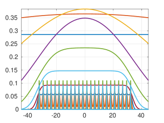
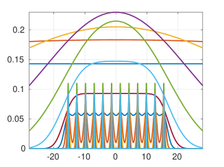
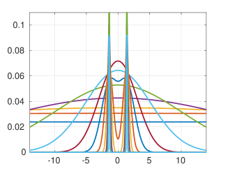
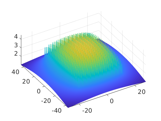
Figure 3.1: Assembled $x$-, $y$- and $z$-axis canonical vectors for a cluster of $24\times 12\times 2$ Hydrogen atoms and the collective 3D electrostatic potential at the cross-section corresponding to one of z-axis layers.

to the summation (assembling) of shifted directional vectors of the canonical tensor representation for a single Newton kernel [39],

$${\bf P}_{c_{L}}=\sum\limits_{q=1}^{R}(\sum\limits_{k_{1}\in{\cal K}}{W}_{({k_{1}})}\widehat{\bf p}^{(1)}_{q})\otimes(\sum\limits_{k_{2}\in{\cal K}}{W}_{({k_{2}})}\widehat{\bf p}^{(2)}_{q})\otimes(\sum\limits_{k_{3}\in{\cal K}}{W}_{({k_{3}})}\widehat{\bf p}^{(3)}_{q}).$$ (3.3)

Here $\widehat{\bf P}$ (similar to (2.11)) represents the single Newton kernel on a twice larger grid and

$${W}_{\nu({\bf k})}={W}_{(k_{1})}\otimes{W}_{(k_{2})}\otimes{W}_{(k_{3})}$$ (3.4)

is the shift-and-windowing (onto $\Omega_{L}$) separable transform along the ${\bf k}$-grid, analogous to the operator (2.12) for direct tensor summation. For rectangular finite 3D lattices the rank of the resulting sum is proven to be the same as for the $R$-term canonical tensor $\widehat{\bf P}$ representing a single Coulomb potential [39].

Figure 3.1 shows the shapes of the assembled canonical vectors for the tensor-based summation of the Hydrogen-nuclei potentials on a rectangular two-layers lattice with of size $24\times 24\times 2$. Left bottom figure shows the electrostatic potential at the cross-section perpendicular to the $z$-axis, which corresponds to the upper layer of the charges.

In the following statement, we generalize this theorem to the case of $d$-dimensional rectangular lattices, thus avoiding the curse of dimensionality.

Theorem 3.1

Given rank-$R$ reference canonical tensor ${\bf P}$, representing a single reference potential, the collective interaction potential $v_{c_{L}}(x)$, $x\in\Omega_{L}$, generated by point potentials on $L^{\otimes d}$ rectangular lattice is presented by the canonical tensor ${\bf P}_{c_{L}}$ of the same rank $R$,

$${\bf P}_{c_{L}}=Z\sum\limits_{q=1}^{R}(\sum\limits_{k_{1}=1}^{L}{\cal W}_{({k_{1}})}{\bf p}^{(1)}_{q})\otimes(\sum\limits_{k_{2}=1}^{L}{\cal W}_{({k_{2}})}{\bf p}^{(2)}_{q})\otimes\cdots\otimes(\sum\limits_{k_{d}=1}^{L}{\cal W}_{({k_{d}})}{\bf p}^{(d)}_{q}),$$ (3.5)

where ${\cal W}_{({k_{\ell}})}$, $\ell=1,\,2,\,\ldots,\,d$ are the shifting-windowing operators for the $d$-dimensional lattice $L\times L\times\cdots\times L$. The numerical cost for evaluation of this potential on $n^{\otimes d}$ tensor grid is estimated by $O(dRLn)$.

The proof is similar to that given in [39], and it is based on separability of the shifting-windowing operator (3.4) on rectangular lattices.

For 3D lattices with multiple vacancies, the tensor rank increases by a small factor [40]. Indeed, for composite geometries the electrostatic potential over defected lattices with simple inclusions can be represented by a sum of low-rank tensors supported on the particular vacancies, ${\cal L}_{q}$, which compose the total lattice ${\cal L}$,

$${\cal L}=\bigcup{\cal L}_{q}.$$

An example of the collective electrostatic potential over a composite lattice with two impurities with different interatomic distances is shown in Figure 3.2. One of the impurities is defined on the sub-lattice of size $3\times 3\times 1$, with a larger positive point charge, while the second one is supported by a sub-lattice of size $3\times 3\times 1$, and contains negative point charges. Further examples can be found in [41], where the assembled tensor summation is discussed in more detail.

In fact, the assembled tensor summation for lattices admits modeling of a number of such impurities since they are all living on the same $n\times n\times n$ 3D Cartesian grid. Then such low-rank canonical tensor representation the collective electrostatic potential enables operations like 3D convolution on 3D grids with $O(n)$ complexity.

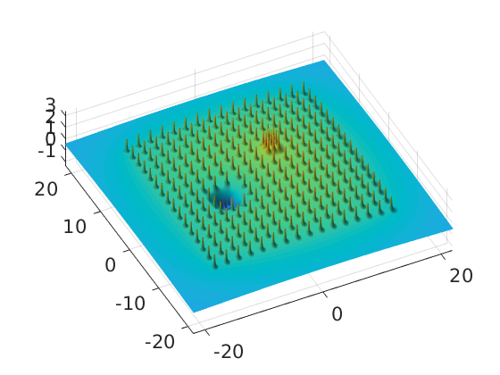
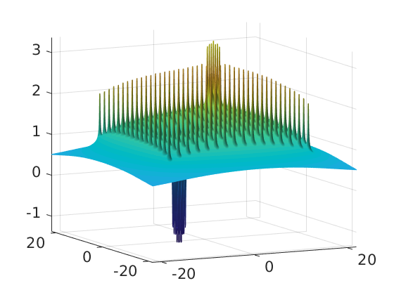
Figure 3.2: A cross-section of the potential at the plane with $z=0$ for the lattice of size $16\times 16\times 1$ with two impurities having different interatomic distances and different charges. The left and right figures show the views from different angles.

$L^{3}$	$64^{3}$	$128^{3}$	$256^{3}$	$512^{3}$
number of particles	262144	2097152	$16\cdot 10^{6}$	$134\cdot 10^{6}$
size in nanometers3	$7^{3}$	$13.4^{3}$	$26.2^{3}$	$51.8^{3}$
$n^{3}$	$4480^{3}$	$8576^{3}$	$16768^{3}$	$33152^{3}$
time	$1.2$	$2.4$	$8.9$	$37.2$
$n^{3}$	$8960^{3}$	$17152^{3}$	$33536^{3}$	$66304^{3}\quad(10^{14})$
time	$1.0$	$4.1$	$18.8$	$84.6$

Table 3.1: Times (sec.) for calculation of the free-space collective electrostatic potential of charged particles placed in nodes of a $L\times L\times L$ 3D lattice vs. the size of representation grid, $n^{3}$.

.

The numerical implementation of the representation (3.5) for the 3D collective electrostatic potential is extremely fast due to the fact that summation of the total potential is reduced to shifting and summation of vectors. Table 3.1 shows the computation times for summation of charges on large 3D lattices composed by nuclei of Hydrogen atoms with an inter-atomic distance of 1 bohr (atomic unit). For example a cluster of $512^{3}$ particles corresponds to a domain size $51.8^{\otimes 3}$ nanometers. We notice, that these calculations are performed in real space (not in the frequency domain).

Now we generalize the previous scheme to the case of variable charges. Consider the 3D case and introduce the three-fold charge tensor ${\bf Z}=\{z_{k_{1},k_{2},k_{3}}\}$, $k_{\ell}=1,\ldots,L$. Assume that tensor ${\bf Z}$ admits the rank-$R_{Z}$ canonical decomposition

$${\bf Z}=\sum\limits_{m=1}^{R_{Z}}{\bf z}^{(1)}_{m}\otimes{\bf z}^{(2)}_{m}\otimes{\bf z}^{(3)}_{m},\quad{\bf z}^{(\ell)}_{m}\in\mathbb{R}^{L}.$$ (3.6)

Consider the weighted electrostatic potential

$$V_{c_{L}}(x)=\sum_{k_{1},k_{2},k_{3}\in{\cal K}}\frac{z_{\bf k}}{\|{x}-a_{1}(k_{1},k_{2},k_{3})\|},\quad x\in\Omega_{L}\in\mathbb{R}^{3},$$ (3.7)

and the corresponding grid-based discretization represented as the canonical tensor

$${\bf P}_{c_{L}}=\sum\limits_{{\bf k}\in{\cal K}^{\otimes 3}}z_{\bf k}{W}_{\nu({\bf k})}\widehat{\bf P}=\sum\limits_{k_{1},k_{2},k_{3}\in{\cal K}}z_{\bf k}{W}_{({\bf k})}\sum\limits_{q=1}^{R}(\widehat{\bf p}^{(1)}_{q}\otimes\widehat{\bf p}^{(2)}_{q}\otimes\widehat{\bf p}^{(3)}_{q})\in\mathbb{R}^{n\times n\times n}.$$

We prove that tensor ${\bf P}_{c_{L}}$ can be calculated in the low-rank canonical format and stored in almost linear cost in $L$, provided that (3.6) holds.

Theorem 3.2

Given the rank-$R$ reference canonical tensor ${\bf P}$ representing the single Newton kernel, the collective interaction potential ${\bf P}_{c_{L}}$ generated by a sum of weighted potentials over $L^{\otimes 3}$ rectangular lattice, where weights ${\bf Z}$ are given in the low-rank form (3.6), can be presented by the canonical rank $\leq R_{Z}R$ tensor

$${\bf P}_{c_{L}}=\sum\limits_{m=1}^{R_{Z}}\sum\limits_{q=1}^{R}(\sum\limits_{k_{1}=1}^{L}z^{(1)}_{m}{\cal W}_{({k_{1}})}{\bf p}^{(1)}_{q})\otimes(\sum\limits_{k_{2}=1}^{L}z^{(2)}_{m}{\cal W}_{({k_{2}})}{\bf p}^{(2)}_{q})\otimes(\sum\limits_{k_{d}=1}^{L}z^{(3)}_{m}{\cal W}_{({k_{3}})}{\bf p}^{(3)}_{q}).$$ (3.8)

The numerical cost for evaluation of the potential (3.8) on $n^{\otimes 3}$ tensor grid is estimated by $O(R_{Z}RLn)$.

Proof. Recall that the separable 3D shift operator is defined by ${\cal W}_{({\bf k})}={\cal W}_{(k_{1})}^{(1)}\otimes{\cal W}_{(k_{2})}^{(2)}\otimes{\cal W}_{(k_{3})}^{(3)}$, ${\bf k}\in\mathbb{Z}^{L\times L\times L}$. Now the representation (3.6) implies

$$\begin{split}{\bf P}_{c_{L}}&=\sum\limits_{q=1}^{R}\sum\limits_{k_{1},k_{2},k_{3}=1}^{L}z_{\bf k}{\cal W}_{(k_{1})}^{(1)}{\bf p}^{(1)}_{q}\otimes{\cal W}_{(k_{2})}^{(2)}{\bf p}^{(2)}_{q}\otimes{\cal W}_{(k_{3})}^{(3)}{\bf p}^{(3)}_{q}\\ &=\sum\limits_{q=1}^{R}\sum\limits_{m=1}^{R_{Z}}\left[(\sum\limits_{k_{1}=1}^{L}z^{(1)}_{m}{\cal W}_{({k_{1}})}{\bf p}^{(1)}_{q})\otimes(\sum\limits_{k_{2},k_{3}=1}^{L}z^{(2)}_{m}{\cal W}_{({k_{2}})}{\bf p}^{(2)}_{q}\otimes z^{(3)}_{m}{\cal W}_{({k_{3}})}{\bf p}^{(3)}_{q})\right]\\ &=\sum\limits_{q=1}^{R}\sum\limits_{m=1}^{R_{Z}}(\sum\limits_{k_{1}=1}^{L}z^{(1)}_{m}{\cal W}_{({k_{1}})}{\bf p}^{(1)}_{q})\otimes(\sum\limits_{k_{2}=1}^{L}z^{(2)}_{m}{\cal W}_{({k_{2}})}{\bf p}^{(2)}_{q})\otimes(\sum\limits_{k_{3}=1}^{L}z^{(3)}_{m}{\cal W}_{({k_{3}})}{\bf p}^{(3)}_{q}).\end{split}$$

This proves the theorem.   

This theorem can be easily generalized to the $d$-dimensional case, cf. Theorem 3.1.

We conclude that the presented method of grid-based assembled tensor summation of the weighted electrostatics potentials represented on $L^{\otimes d}$ lattice can be performed at the numerical cost and storage size bounded by $O(dR_{Z}RLn)$ and $O(dR_{Z}Rn)$, respectively.

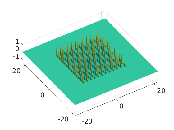
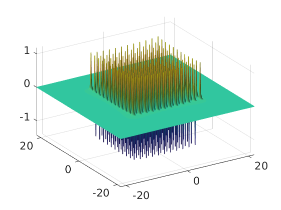
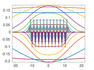
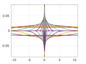
Figure 3.3: Collective 3D electrostatic potential modeling one-layer dipole-type system including $12\times 12\times 1$ positive and $11\times 11\times 1$ negative charges. Bottom figures show the $x$- and $z$-axis canonical vectors for this cluster.

Figure 3.3 presents the electrostatic potential of a dipole-type lattice with positive and negative charges mixed in a checkerboard order, see top figures. In this example the charge configuration is represented by rank-$2$ tensor array. Bottom figures show shapes of the assembled canonical vectors resulted by the tensor-based summation of the potentials on a lattice. One can distinguish separate picks for positive and negative contributions. The values of the negative charges are chosen to provide a neutral system.

3.3 Interaction energy of charged particles on 3D lattices

Notice that the traditional approaches, like Ewald-type summation [20] exhibit $O(L^{3}\log L)$ complexity for the energy calculations on $L\times L\times L$ 3D lattice. In turn calculation of the interaction energy of equally charged particles in 3D case by using tensor representation of the collective potential scales linearly in $L$ [39]. In this section we consider this issue in the more general setting.

The interaction energy of charged particles in a $L\times L\times L$ lattice is given by

$$E_{nuc}=\frac{1}{2}\sum^{L^{3}}_{i=1}\sum^{L^{3}}_{j=1,j\neq i}\frac{z_{i}z_{j}}{\|x_{i}-x_{j}\|},\quad x_{i},x_{j}\in\mathbb{R}^{3},$$

where $z_{i}$ and $z_{j}$ are the particle charges and $x_{i}$ and $x_{j}$ are their coordinates. $O(3RL)\ll L^{3}\log L$ Recall that the interaction energy of a systems of equal-charged particles in a lattice can be efficiently calculated by using the collective electrostatic potential of a lattice-type computed using the assembled vectors of the canonical (or Tucker) tensor representation of the Newton kernel.

Given $\widetilde{\bf P}_{c_{L}}$ that is the trace of the (rescaled by the factor $h^{3}$) collective potential ${\bf P}_{c_{L}}$ onto the lattice points, and denote the all-ones tensor of the same size by ${\bf 1}$, then the energy sum with accuracy $O(h^{2})$ is computed as (see [39])

$$E_{L,T}=\frac{Z^{2}}{2}(\langle\widetilde{\bf P}_{c_{L}},{\bf 1}\rangle-\sum\limits_{{\bf k}\in{\cal K}}{\bf P}_{|x_{\bf k}=0}),$$

where $Z$ is the point charge. Finally, by introducing the rank-$1$ tensor ${\bf P}_{0L}={\bf P}_{|x_{\bf k}=0}{\bf 1}$, we represent the interaction energy $E_{L,T}$ by a simple tensor operation

$$E_{L,T}=\frac{Z^{2}}{2}(\langle\widetilde{\bf P}_{c_{L}},{\bf 1}\rangle-\langle{\bf P}_{0L},{\bf 1}\rangle),$$ (3.9)

which can be implemented in $O(3RL)\ll L^{3}\log L$ complexity. Indeed, Theorem 3.1 implies that the tensor $\widetilde{\bf P}_{c_{L}}$ has the canonical rank not larger than $R$.

Likewise, in the case of variable charges, Theorem 3.2 justifies that the canonical rank of the corresponding collective potential $\widetilde{\bf P}_{c_{L}}$ does not exceed $R_{Z}R$. Hence, in this case the representation (3.9) takes the form

$$E_{L,T}=\frac{1}{2}(\langle\widetilde{\bf P}_{c_{L}},{\bf Z}\rangle-{\bf P}_{|x_{\bf k}=0}\langle{\bf Z},{\bf Z}\rangle),$$ (3.10)

which can be evaluated in $O(3R_{Z}RL)$ operations. The above arguments prove the following result.

Theorem 3.3

Given the tensor $\widetilde{\bf P}_{c_{L}}$, in the case of constant charges on the $L\times L\times L$-lattice the interaction energy of the lattice-structured system is calculated by (3.9) in the linear cost in $L$, $O(3RL)$. In the case of variable charge distributions with the charges given by a rank-$R_{Z}$ tensor, the interaction energy of the lattice-structured system is calculated by (3.10) at the expense $O(3R_{Z}RL)$.

Table 3.2 shows CPU times for computation of the interaction energy ($Z=1$) for several cubic clusters of charged particles using Matlab. Time T_full denotes the time for direct $O(L^{6})$ computations, while $T_{(L^{3})}$ presents the square root of this time, to show the $O(L^{3})$ complexity (restricted to $L=48$). The column T_tens. shows the times for tensor-based calculations.

$L^{3}$	Tfull $T_{(L^{3})}$	Ttens.	$E_{L,T}$	abs. err.
$32^{3}$	$250$, ($15.8$)	$1.5$	$1.5\cdot 10^{7}$	$1.5\cdot 10^{-9}$
$48^{3}$	$3374$, ($58.8$)	$2.8$	$1.12\cdot 10^{8}$	0
$64^{3}$	–	$5.7$	$5.0\cdot 10^{8}$	–
$128^{3}$	–	$13.5$	$1.6\cdot 10^{10}$	–
$256^{3}$	–	$68.2$	$5.2\cdot 10^{11}$	–

Table 3.2: Comparison of calculation times for computation of the interaction energy for increasing cluster size.

4 Tensor representation of multi-particle potentials

4.1 How to treat systems of generally distributed particles

What if a many-particle system is not of lattice-type, but is unstructured like a protein? Then summation of many canonical tensors

$$P_{0}(x)\mapsto{\bf P}_{0}=\sum_{\nu=1}^{N_{0}}{z_{\nu}}\,{\cal W}_{\nu}(\widehat{\bf P}_{R}).$$ (4.1)

yields large canonical ranks, like in direct tensor summation (see Section 2.2) when the number of particles increases (”a non-structured system“).

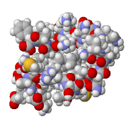
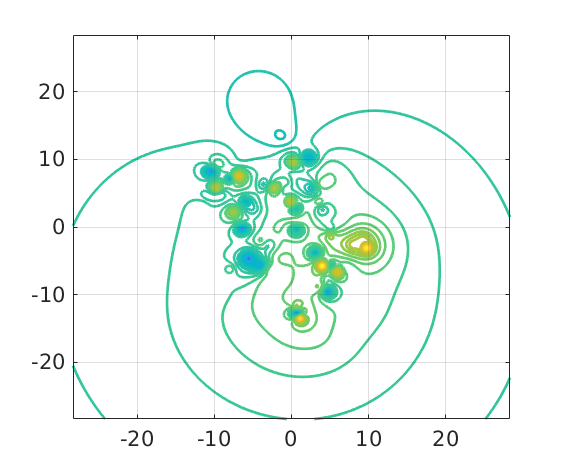
Figure 4.1: Left: a typical structure of moderate size protein molecule; right: the equi-potential contours of the total electrostatic potential of a protein-type molecule with 200 nuclei visualized at the plane with $z=0$.

Figure 4.1, left demonstrates the structure of a villin protein [6] and the level set for the collective electrostatic potential. We notice that at the lower values of potential the contours are smooth and unite large groups of particles, while at the vicinity of singularities we observe high density of levels. This observation advocates the idea to separate the low-level part of the collective potential.

Figure 4.2 illustrates the mode-$1$ singular values of the RHOSVD of the side matrices for the full potential of the protein-type system (left) and of its low-range parts (right) versus the number of particles $N_{0}=200,400,774$ , $n=1024$.

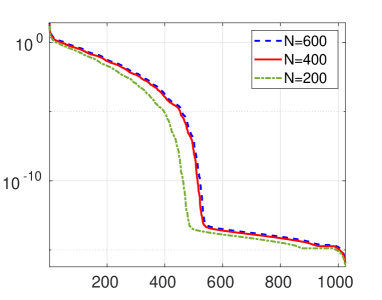
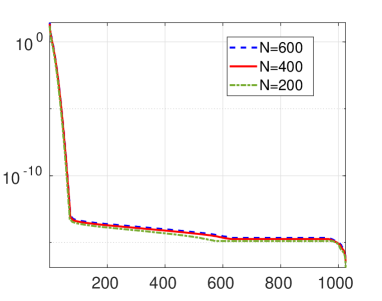
Figure 4.2: The singular values of the mode-$1$ RHOSVD for the large sum of Newton kernels.

This example indicates that in the case of a non-structured location of particles the Tucker/canonical rank of the corresponding grid-based tensor representation of the collective potential increases proportionally to the number of particles. The large ranks make the tensor decomposition of the full electrostatic potential of a the biomolecules useless. The application of the range separated tensor decompositions allows to get rid of this bottleneck.

4.2 Range-separated tensor splitting of the generating kernel

From the detailed consideration of the quadrature (2.7), we can observe that the full set of approximating Gaussians includes two classes of functions: those with small ”effective support” and the long-range functions. Consequently, functions from different classes may require different tensor-based schemes for their efficient numerical treatment. Hence, the idea of the new approach is the constructive implementation of a range separation scheme that allows the independent efficient treatment of both the long- and short-range parts in each summand in (2.10).

In what follows, without loss of generality, we confine ourselves to the case of the Newton kernel in $\mathbb{R}^{3}$, that is represented by the canonical sum in (2.7) with $k=0,1,\ldots,M_{0}$, $M_{0}=2M+1$. We observe that the sequence of quadrature points $\{t_{k}\}$, can be split into two subsequences, ${\cal T}:=\{t_{k}|k=0,1,\ldots,M_{0}\}={\cal T}_{l}\cup{\cal T}_{s},$ with

$${\cal T}_{l}:=\{t_{k}\,|k=0,1,\ldots,R_{l}\},\quad\mbox{and}\quad{\cal T}_{s}:=\{t_{k}\,|k=R_{l}+1,\ldots,M_{0}\}.$$ (4.2)

Here ${\cal T}_{l}$ includes quadrature points $t_{k}$ condensed “near” zero (more precisely, in the interval $(0,1]$), hence generating the long-range Gaussians (low-pass filters). In turn, ${\cal T}_{s}$ accumulates the increasing in $M\to\infty$ sequence of “large” sampling points $t_{k}$ (more precisely, in the interval $(1,\infty)$), with the upper bound $C_{0}^{2}\log^{2}(M)$, corresponding to the short-range Gaussians (high-pass filters). We further denote ${\cal K}_{l}:=\{k\,|t_{k}\in{\cal T}_{l}\}$ and ${\cal K}_{s}:=\{k\,|t_{k}\in{\cal T}_{s}\}$.

Splitting (4.2) generates the additive decomposition of the canonical tensor $\mathbf{P}_{R}$ onto the short- and long-range parts,

$$\mathbf{P}_{R}=\mathbf{P}_{R_{s}}+\mathbf{P}_{R_{l}},$$

where

$$\mathbf{P}_{R_{s}}=\sum\limits_{k\in{\cal K}_{s}}{\bf p}^{(1)}_{k}\otimes{\bf p}^{(2)}_{k}\otimes{\bf p}^{(3)}_{k},\quad\mathbf{P}_{R_{l}}=\sum\limits_{k\in{\cal K}_{l}}{\bf p}^{(1)}_{k}\otimes{\bf p}^{(2)}_{k}\otimes{\bf p}^{(3)}_{k}.$$ (4.3)

The choice of the critical number $R_{l}=\#{\cal T}_{l}-1$ (or equivalently, $R_{s}=\#{\cal T}_{s}=M-R_{l}$), that specifies the splitting ${\cal T}={\cal T}_{l}\cup{\cal T}_{s}$, is determined by the active support of the short-range components such that one can cut off the functions ${\bf p}_{k}(x)$, $t_{k}\in{\cal T}_{s}$, outside of the sphere $B_{\sigma}$ of radius ${\sigma}>0$, subject to a certain threshold $\delta>0$. Fixed $\delta>0$, the choice of $R_{s}$ is defined by the (small) parameter $\sigma$ and vise versa, see [2] for further details.

For example, in electronic structure calculations, the parameter $\sigma$ can be associated with the typical inter-atomic distance in the molecular system of interest.

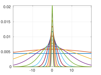
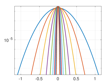
Figure 4.3: Long-range vectors (left) and short-range (in logarithmic scale) canonical vectors for the Newton kernel with $n=1024$, $R=24,R_{l}=13$.

Figure 4.3 illustrates the splitting (4.2) for the tensor ${\bf P}_{R}={\bf P}_{R_{l}}+{\bf P}_{R_{s}}$ in (4.3) represented on the $n\times n\times n$ grid with the parameters $R=20,R_{l}=12$ and $R_{s}=8$, respectively (cf. [2]). The canonical vectors of the discretized Newton kernel depicted in Figure 4.3, left, exhibit long-range behavior, while the corresponding vectors of the tensor ${\bf P}_{R_{s}}$ decay exponentially fast apart of the effective support, see Figure 4.3, right.

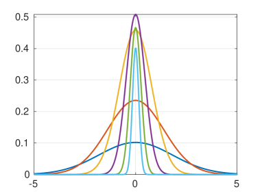
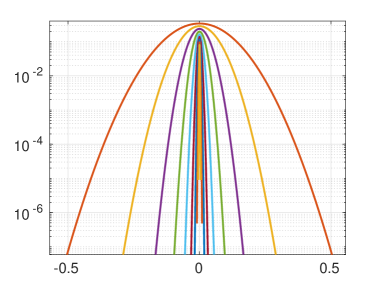
Figure 4.4: Long-range (left) and short-range (right) mode-1 canonical vectors for the 3D Slater function with $n=1024$, $R=24,R_{l}=6$. Short-range vectors are shown in logarithmic scale.

Figure 4.4 illustrates the splitting (4.2) for the tensor ${\bf P}_{R}={\bf P}_{R_{l}}+{\bf P}_{R_{s}}$ in (4.3) representing the Slater potential $P(x)=e^{-\|x\|}$ on the $n\times n\times n$ grid with the parameters $R=24,R_{l}=6$ and $R_{s}=18$. Notice that for this radial function the long-range part (Figure 4.4, left) includes much less canonical vectors compared with the case of Newton kernel. This anticipates the smaller total canonical rank for the long-range part in the large sum of Slater-like potentials arising, for example, in the representation of molecular orbitals and the electron density in electronic structure calculations. For instance, the wave function for the Hydrogen atom is given by the Slater function $e^{-\mu\|x\|}$, $x\in\mathbb{R}^{3}$.

The advantage of the range separation in the splitting of the canonical tensor in (4.3) is due to the opportunity for independent tensor representations of both sub-tensors ${\bf P}_{R_{s}}$ and ${\bf P}_{R_{l}}$ providing the separate grid-based treatment of the short- and long-range parts in the total sum of many pointwise interaction potentials as in (2.10).

4.3 Brief introduction to the RS tensor format

The novel range separated (RS) tensor format has been recently introduced in [2]. This format is well suited for modeling of the long-range interaction potential in multi-particle systems, as well as for the low-parametric interpolation of the scattered data. It is based on the partitioning of the tensor representation of the reference kernel (usually the radial basis function) into long- and short-range parts.

First, we recall the general definition of the RS tensor format

Definition 4.1

(RS-canonical tensors [2]). Given the separation parameter $\gamma\in\mathbb{N}$ and a set of points $x_{\nu}\in\mathbb{R}^{d}$, $\nu=1,\ldots,N$, the RS-canonical tensor format specifies the class of $d$-tensors ${\bf A}\in\mathbb{R}^{n_{1}\times\cdots\times n_{d}}$ which can be represented as a sum of a rank-${R}_{L}$ canonical tensor

$${\bf A}_{R_{L}}={\sum}_{k=1}^{R_{L}}\xi_{k}{\bf a}_{k}^{(1)}\otimes\cdots\otimes{\bf a}_{k}^{(d)}\in\mathbb{R}^{n_{1}\times...\times n_{d}}$$ (4.4)

and a cumulated canonical tensor $\widehat{\bf A}_{S}={\sum}_{\nu=1}^{N}c_{\nu}{\bf A}_{\nu},$ generated by replication of the reference tensor ${\bf A}_{0}$ to the predefined points $x_{\nu}$, $\nu=1,\ldots,N$. Then the RS canonical tensor is parametrized by

$${\bf A}={\bf A}_{R_{L}}+\widehat{\bf A}_{S}={\sum}_{k=1}^{R_{L}}\xi_{k}{\bf a}_{k}^{(1)}\otimes\cdots\otimes{\bf a}_{k}^{(d)}+{\sum}_{\nu=1}^{N}c_{\nu}{\bf A}_{\nu},$$ (4.5)

where $\mbox{rank}({\bf A}_{0})\leq R_{0}$ and $\mbox{diam}(\mbox{supp}{\bf U}_{0})\leq 2\gamma$ in the index size.

The storage size for the RS-canonical tensor ${\bf A}$ in (4.5) is estimated by ([2], Lemma 3.9),

$$\mbox{stor}({\bf A})\leq dRn+(d+1)N+dR_{0}\gamma.$$

The RS-Tucker tensor format is defined similar to Definition 4.1 such that the rank-$R_{L}$ canonical tensor (4.4) is substituted by the rank-$(r_{1},\ldots,r_{d})$ Tucker tensor.

The RS-canonical and Tucker tensor formats provide the powerful tool for data-sparse rank-structured representation of many-particle electrostatic potentials. In what follows we consider the basic example of the free space electrostatic potential of large system of charged particles.

According to the tensor canonical representation of the Newton kernel (2.7) as a sum of Gaussians, one can distinguish their supports into the short- and long-range parts, $\mathbf{P}_{R}=\mathbf{P}_{R_{s}}+\mathbf{P}_{R_{l}},$ given by (4.3). Then the RS splitting (4.3) is applied to the reference canonical tensor ${\bf P}_{R}$ and to its accompanying version $\widetilde{\bf P}_{R}=[\widetilde{p}_{R}(i_{1},i_{2},i_{3})]$, $i_{\ell}\in\widetilde{I}_{\ell}$, $\ell=1,2,3$ living on the double size grid with the same mesh width, such that

$$\widetilde{\bf P}_{R}=\widetilde{\mathbf{P}}_{R_{s}}+\widetilde{\mathbf{P}}_{R_{l}}\in\mathbb{R}^{2n\times 2n\times 2n}.$$

The total electrostatic potential $P_{0}(x)$ in (4.1) is represented by a projected tensor ${\bf P}_{0}\in\mathbb{R}^{n\times n\times n}$ that can be constructed by a direct sum of shift-and-windowing transforms of the reference tensor $\widetilde{\bf P}_{R}$ (see [39] for more details),

$${\bf P}_{0}=\sum_{\nu=1}^{N}{z_{\nu}}\,{\cal W}_{\nu}(\widetilde{\bf P}_{R})=\sum_{\nu=1}^{N}{z_{\nu}}\,{\cal W}_{\nu}(\widetilde{\mathbf{P}}_{R_{s}}+\widetilde{\mathbf{P}}_{R_{l}})=:{\bf P}_{s}+{\bf P}_{l}.$$ (4.6)

The shift-and-windowing transform ${\cal W}_{\nu}$ maps a reference tensor $\widetilde{\bf P}_{R}\in\mathbb{R}^{2n\times 2n\times 2n}$ onto its sub-tensor of smaller size $n\times n\times n$, obtained by first shifting the center of the reference tensor $\widetilde{\bf P}_{R}$ to the grid-point $x_{\nu}$ and then restricting (windowing) the result onto the computational grid $\Omega_{n}$.

The disadvantage of the tensor representation (4.6) is that the number of terms in the canonical representation of the full tensor sum ${\bf P}_{0}$ increases almost proportionally to the number $N$ of particles in the system.

The remedy was found in [2] by considering the global tensor decomposition of only the ”long-range part” in the tensor ${\bf P}_{0}$, defined by

$${\bf P}_{l}=\sum_{\nu=1}^{N}{z_{\nu}}\,{\cal W}_{\nu}(\widetilde{\mathbf{P}}_{R_{l}})=\sum_{\nu=1}^{N}{z_{\nu}}\,{\cal W}_{\nu}(\sum\limits_{k\in{\cal K}_{l}}\widetilde{\bf p}^{(1)}_{k}\otimes\widetilde{\bf p}^{(2)}_{k}\otimes\widetilde{\bf p}^{(3)}_{k}).$$ (4.7)

The tensor representation of the sum of short-range parts is given by a sum of cumulative tensors of small support (and small size), accomplished by the list of the 3D potentials coordinates.

In application to the calculation of multi-particle interaction potentials discussed above we associate the tensors ${\bf P}_{s}$ and ${\bf P}_{l}$ in (4.6) with short- and long-range components ${\bf A}_{R_{L}}$ and $\widehat{\bf A}_{S}$ in the RS representation of the collective electrostatic potential ${\bf P}_{0}$. The following theorem proofs the almost uniform in $N$ bound on the Tucker (and canonical) $\varepsilon$-rank of the tensor ${\bf A}_{R_{L}}={\bf P}_{l}$, representing the long-range part of ${\bf P}_{0}$.

Theorem 4.2

(Uniform rank bounds for the long-range part, [2]). Let the long-range part ${\bf P}_{l}$ in the total interaction potential, see (4.7), correspond to the choice of splitting parameter in (4.2) with $M_{0}=O(\log^{2}\varepsilon)$. Then the total $\varepsilon$-rank ${\bf r}_{0}$ of the Tucker approximation to the canonical tensor sum ${\bf P}_{l}$ is bounded by

$${\bf r}_{0}:=\mbox{rank}_{Tuck}({\bf P}_{l})=C\,b\,\log^{3/2}(|\log(\varepsilon/N)|),$$ (4.8)

where the constant $C$ does not depend on the number of particles $N$, as well as on the size of the computational box, $[-b,b]^{3}$.

The estimate (4.8) indicates that for fixed size of computational box embedding the many-particle system the numerical cost for the canonical approximation of the long range part in the collective potential depends only logarithmically on the approximation accuracy and the number of particles.

Corollary 4.3

The simple consequence of Theorem 4.2 is the following estimate on the CP rank and the TT-rank of the long-range part in the collective electrostatic potential ${\bf P}_{l}$,

$$\mbox{rank}_{CP}({\bf P}_{l})\leq{\bf r}_{0}^{2},\quad\mbox{rank}_{TT}({\bf P}_{l})\leq{\bf r}_{0}^{2},$$

where the Tucker rank ${\bf r}$ is bounded by (4.8).

Numerical rank reduction in the sum (4.7) with the initial canonical rank $R_{0}=RN$ is performed by the C2T algorithm that is based on the SVD of the $n\times R_{0}$ side matrices in the canonical sum (4.7). In case of very large number of particles $N$ the C2T algorithm can be applied in the “add-and-compress” version. In this approach the initial group of $N$ particles is decomposed into certain number $m_{0}$ of small subgroups such that the long-range part is precomputed for each subgroup and then rank compression applies to the sum of $m_{0}$ canonical tensors with a small rank. The optimal number $m_{0}$ can be easily estimated by solving simple optimization problem for the cost functional.

5 RS tensor format in bio-molecular modeling

5.1 Interaction energy and forces via long-range part in the potential

The RS tensor format introduced in [2] applies to many particle systems with rather generally located potentials all discretized on the fine tensor grid in $\mathbb{R}^{3}$. These can be the electrostatic potentials of large atomic systems like bio-molecules or the multidimensional scattered data modeled by radial basis functions. The main advantage of the RS tensor format is that the partition into the long- and short-range parts is performed just by sorting skeleton vectors in the tensor representation of the generating kernel,

$$\mathbf{P}_{R}=\mathbf{P}_{R_{s}}+\mathbf{P}_{R_{l}}.$$

Theorem 4.2 proves that the sum of long range contributions from all particles in the collective potential is represented by a low-rank canonical/Tucker tensor with a rank which only logarithmically depends on the number of particles $N$. The representation complexity of the short range part is $O(N)$ with a small constant independent on the number of particles.

The basic tool for fast calculation of the long-range part is the canonical-to-Tucker algorithm combined with the reduced higher order SVD (RHOSVD), see [47]. The error of the RS tensor representation is defined by the $\varepsilon$-truncation threshold for the Tucker-to-canonical algorithm in the rank reduction scheme. Figure 5.1 illustrates the cross-sections of the collective free space electrostatic potential for $650$ atomic biomolecule [50] computed by the RS tensor representation.

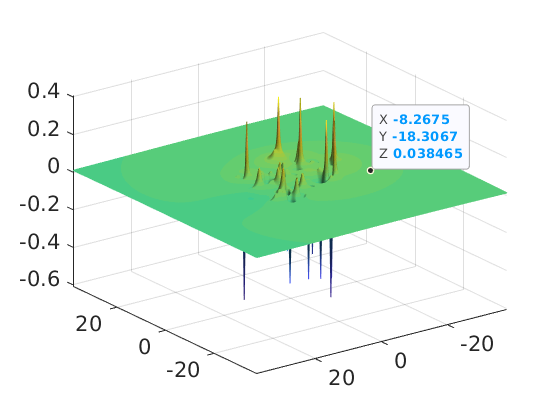
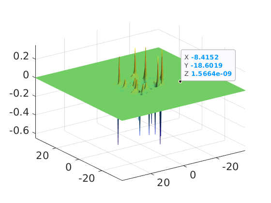
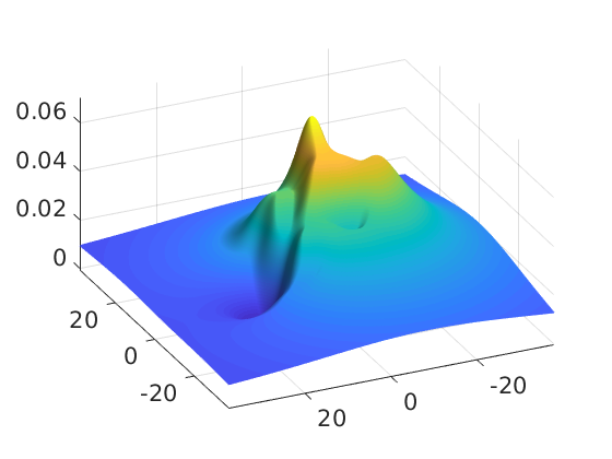
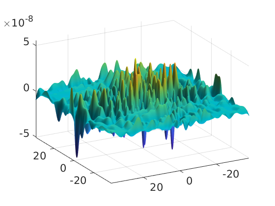
Figure 5.1: Top: Left: the free space electrostatic potential of a small biomolecule computed by RS tensor format. Right: the short-range part of the RS tensor. Bottom: The long-range part of the collective free space electrostatic potential of a small biomolecule (left) and the error of RS representation (right).

The beneficial feature of the RS decomposition is due to the low-parametric grid-based representation of the long-range component in the many-particle potential which allows to recover the most important physical characteristic of the system such that the interaction energy and forces. Recall that the electrostatic interaction energy is represented in the form

$$E_{N}=E_{N}(x_{1},\dots,x_{N})=\sum^{N}_{i=1}\sum^{N}_{j<i}\frac{z_{i}z_{j}}{\|x_{i}-x_{j}\|},$$ (5.1)

and it can be computed by direct summation in $O(N^{2})$ operations. Define vectors ${\bf z}=(z_{1},\ldots,z_{N})^{T}\in\mathbb{R}^{N}$ and ${\bf p}_{l}=({\bf P}_{l}({x}_{1}),\ldots,{\bf P}_{l}({x}_{N})0^{T}\in\mathbb{R}^{N}$. Given the long-range tensor representation ${\bf P}_{l}$, the following lemma represents the electrostatic interaction energy by simple operation with the vectors ${\bf z}$ and ${\bf p}_{l}$ which can be precomputed at $O(N)$ cost up to lower order terms. The following statement is the minor modification of Lemma 4.2 in [2].

Lemma 5.1

Let the effective support of the short-range components in the reference potential ${\bf P}_{R}$ do not exceed $\sigma>0$. Then the interaction energy $E_{N}$ of the $N$-particle system can be calculated by using only the long range part in the total potential sum

$$E_{N}=\frac{1}{2}\sum\limits_{{j}=1}^{N}z_{j}({\bf P}_{l}({x}_{j})-z_{j}{\bf P}_{R_{l}}(0))=\frac{1}{2}\langle{\bf z},{\bf p}_{l}\rangle-\frac{{\bf P}_{R_{l}}(0)}{2}\sum\limits_{{j}=1}^{N}z_{j}^{2},$$ (5.2)

in $O(dR_{l}N)$ operations, where $R_{l}$ is the canonical rank of the long-range component.

Here the term $\frac{1}{2}\langle{\bf z},{\bf p}_{l}\rangle$ denotes the ”non-calibrated” interaction energy with the long-range tensor component ${\bf P}_{l}$. Lemma 5.1 indicates that the interaction energy does not depend on the short-range part in the collective potential which is the key point for the construction of energy preserving regularized numerical schemes for solving the basic equations in bio-molecular modeling.

Notice that the energy expansion (3.9) is the particular version of (5.2) in the case of lattice structured system with equal charges.

The other important application of the RS format is due to the opportunity to recompute gradients and the force field at each particle location of interest in applications to multi-particle dynamics. In particular, such computational tasks arise in the problem of protein-ligand docking, in the process of electrostatic self-assembly, and for the general use in many-particle classical dynamics.

Calculation of electrostatic forces and gradients of the interaction potentials in multiparticle systems is a computationally extensive problem. The algorithms based on Ewald summation technique were discussed in [16, 30]. We propose an alternative approach using the RS tensor format.

First, we consider the gradients operator. Given an RS-canonical tensor ${\bf A}$ as in (4.5) with the width parameter $\gamma>0$, the discrete gradient $\nabla_{h}=(\nabla_{1},\ldots,\nabla_{d})^{T}$ applied to the long-range part in ${\bf A}={\bf A}_{s}+{\bf A}_{l}$ at all grid points of $\Omega_{h}$ simultaneously, can be calculated as the $R$-term canonical tensor by applying the simple one-dimensional finite-difference (FD) operations to each rank-$1$ term in the long-range part ${\bf A}_{l}$,

$$\nabla_{h}{\bf A}_{l}={\sum}_{k=1}^{R}\xi_{k}({\bf G}_{k}^{(1)},\ldots,{\bf G}_{k}^{(d)})^{T},$$ (5.3)

with rank-$1$ tensor entries ${\bf G}_{k}^{(\ell)}={\bf a}_{k}^{(1)}\otimes\cdots\otimes\nabla_{\ell}{\bf a}_{k}^{(\ell)}\otimes\cdots\otimes{\bf a}_{k}^{(d)},$ where $\nabla_{\ell}$ ($\ell=1,\dots,d$) is the univariate FD differentiation scheme in variable $x_{\ell}$ (by using backward or central differences). Numerical complexity of the representation (5.3) can be estimated by $O(dRn)$ provided that the canonical rank is almost uniformly bounded in the number of particles. The gradient operator applies locally to each short-range term in (4.5) which amounts in the complexity $O(dR_{0}N)$.

Given the electrostatic potential energy $E_{N}$, the force vector ${\cal F}_{j}$ on the particle $j$ is obtained by differentiating the functional $E_{N}(x_{1},\dots,x_{N})$ with respect to $x_{j}$,

$${\cal F}_{j}=-\frac{\partial}{\partial x_{j}}E_{N}=-\nabla_{|x_{j}}E_{N},$$

which can be calculated explicitly (see [30]) in the form,

$${\cal F}_{j}=\frac{1}{2}z_{j}\sum\limits_{{k}=1,{k}\neq{j}}^{N}z_{k}\frac{{x}_{j}-{x}_{k}}{\|{x}_{j}-{x}_{k}\|^{3}}.$$ (5.4)

The Ewald summation technique for force calculations on the positions of particles was discussed for example in [16, 30].

As an alternative to the direct summation by (5.4) we discuss two diffent approaches for fast evaluation of (5.4) based on the the RS tensor representation.

(A) The RS tensor approximation can be applied directly to the discretized electric field on the potential $P_{0}$, that is a sum of dipole-like terms,

$${\cal E}(x)=-\nabla P_{0}(x)=\sum\limits_{{k}=1}^{N}z_{k}\frac{{x}-{x}_{k}}{\|{x}-{x}_{k}\|^{3}}.$$

This approach will be considered elsewhere.

(B) Calculation the force field components ${\cal F}_{j}$ by the direct FD numerical differentiation of the energy functional $E_{N}$ by using RS tensor representation of the long-range part in the $N$-particle interaction potential $P_{0}(x)$ discretized on fine spacial grid (see [2]).

In approach (B), the differentiation in RS-tensor format with respect to $x_{j}$ is based on the explicit representation (5.2) which requires only the calculation of long-range tensor ${\bf P}_{l}$. We chose $j=N$ for example, and apply the FD differentiation to the energy representation (5.2) to obtain

$$E_{N}(x_{1},\dots,x_{N})-E_{N}(x_{1},\dots,x_{N}-h{\bf e}_{i})=\frac{1}{2}\langle{\bf z},{\bf p}_{l}(x_{1},\dots,x_{N})-{\bf p}_{l}(x_{1},\dots,x_{N}-h{\bf e}_{i})\rangle,$$

for three different values of the axis vectors ${\bf e}_{1}=(1,0,0)^{T}$, ${\bf e}_{2}=(0,1,0)^{T}$ and ${\bf e}_{3}=(0,0,1)^{T}$. The implementation needs a simple recalculation of the smooth potential ${\bf P}_{l}$ under small variation of the only one particle center $x_{N}$ leading to the cost $O(dRn)$, uniformly in $N$.

The energy and force field calculus discussed above are related to the free space electrostatic potential. The case of bio-molecular simulations, the protein like structures are modeled by solute-solvent systems in polarizable media, where substructures with different permeability constants are included. The electrostatics in such systems is most commonly described by the linear (or nonlinear) Poisson-Boltzmann equation to be addressed in what follows.

5.2 The linearized Poisson-Boltzmann equation

The Poisson-Boltzmann equation (PBE) describes the electrostatic potential of an ensemble of charged particles immersed in a continuum dielectric medium with fixed permittivity $\epsilon_{s}$ provided that each charge is embedded into a small sphere with different from $\epsilon_{s}$ dielectric constant. The PBE can be formulated either as the elliptic partial differential equation in $\mathbb{R}^{3}$ [31, 9], or as the boundary integral equation over the solute-solvent interface [8, 55, 73] (in the case of linear model in $\mathbb{R}^{3}$). The PBE model is supposed to capture the polarization effects in many-body systems.

The basic techniques on the analysis and numerical approximation of the boundary and volume integral equations have been addressed in [59, 32, 67]. The commonly used techniques for solving the arising discretized elliptic equations in $\mathbb{R}^{3}$ are based on either multigrid iteration [31] or domain decomposition methods [56, 9].

The linearized PBE in the differential form reads as the elliptic boundary value problem

$$-\nabla\cdot(\epsilon\nabla u)+\kappa^{2}u=\rho_{f}:={\sum}_{{k}=1}^{N}z_{k}\delta({x}-{x}_{k})\quad\mbox{in }\quad\Omega=\Omega_{s}\cup\Omega_{m},$$ (5.5)

where $u$ is the target electrostatic potential of a protein, $\rho_{f}$ is the scaled singular charge distribution (here $\delta(x)$ is the Dirac delta) supported at points $x_{k}\in\Omega_{m}$ in the solute region, where $\epsilon=\epsilon_{m}$ and $\kappa=0$, while in the external solvent domain $\Omega_{s}$ we have $\kappa\geq 0,\epsilon=\epsilon_{s}$. The interface conditions arise from the continuity of the potential and flaxes on $\Gamma=\partial\Omega_{m}$: $[u]_{\Gamma}=0,\;\left[\epsilon\frac{\partial u}{\partial n}\right]_{\Gamma}=0\;\mbox{on}\;\Gamma.$ Moreover, the trace of the solution on $\partial\Omega$ or some other quantities may be fixed.

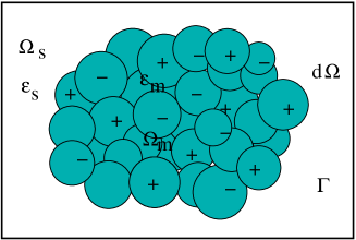
Figure 5.2: Computational domain for the PBE.

The traditional FEM discretization methods could not be applied directly to the equation (5.5) because the lack of regularity in the solution $u$. The traditional approaches are merely based on the regularization of this equation by subtraction of the exact free space electrostatic potential that solves the linear equation $-\Delta u_{0}=\rho_{f}$ in $\mathbb{R}^{3}$. Such approaches require the essential modification of the interface and boundary conditions, as well as the non-trivial (especially in the nonlinear case) recovery procedure of the total interaction energy since the component $u_{0}$ may include considerable portion of energy.

In what follows we discuss the recently introduced new energy preserving regularization scheme based on (A) the RS splitting of the discretized Dirac delta [45], and (B) using the RS tensor format [2] for the construction of the regularized solution [45, 3, 50].

5.3 The RS tensor decomposition of the discretized Dirac delta

The RS tensor splitting of the discretized Dirac delta introduced in [45] is based on the idea that discretized Dirac delta can be recovered from the governing equation

$$-\Delta\frac{1}{\|x\|}=4\pi\delta(x),\quad x\in\mathbb{R}^{3},$$ (5.6)

discretized on the fine tensor grid in the computational box in $\mathbb{R}^{3}$. Indeed, we can discretize all entities on the left hand side of the equation (5.6) via grid-based approximations which admit the low-rank representations as follows

$$\frac{1}{\|x\|}\rightsquigarrow\mathbf{P}_{R}=\mathbf{P}_{R_{s}}+\mathbf{P}_{R_{l}}\in\mathbb{R}^{n\times n\times n},\quad\mbox{and}\quad\Delta\rightsquigarrow{\Delta}_{h},$$

where ${\Delta}_{h}$ is the finite difference (FD) Laplacian over $n\times n\times n$ grid with mesh size $h$. In particular, we use the Kronecker rank-$3$ representation

$${\Delta}_{h}=\Delta_{1}\otimes I_{2}\otimes I_{3}+I_{1}\otimes\Delta_{2}\otimes I_{3}+I_{1}\otimes I_{2}\otimes\Delta_{3}.$$ (5.7)

This introduces the grid representation of the Dirac delta

$$\delta(x)\rightsquigarrow\boldsymbol{\delta}_{h}:=-\frac{1}{4\pi}{\Delta}_{h}\mathbf{P}_{R},$$ (5.8)

which is associated with its particular differential representation (5.6). Now the rank-$3R$ CP tensor representation $\boldsymbol{\delta}_{h}$ of the discretized Dirac delta ${\delta}$ approximated on $n\times n\times n$ Cartesian grid can be computed as the action of the Laplace operator on the Newton kernel given in the canonical rank-$R$ tensor format as follows

$$\boldsymbol{\delta}_{h}=-A_{\Delta}\mathbf{P}_{R}=\sum\limits_{k=1}^{R}(\Delta_{1}{\bf p}^{(1)}_{k}\otimes{\bf p}^{(2)}_{k}\otimes{\bf p}^{(3)}_{k}+{\bf p}^{(1)}_{k}\otimes\Delta_{2}{\bf p}^{(2)}_{k}\otimes{\bf p}^{(3)}_{k}+{\bf p}^{(1)}_{k}\otimes{\bf p}^{(2)}_{k}\otimes\Delta_{3}{\bf p}^{(3)}_{k}).$$

The short- and long-range splitting of the discretized $\boldsymbol{\delta}_{h}$ is defined by

$$\boldsymbol{\delta}_{h}=\boldsymbol{\delta}_{s}+\boldsymbol{\delta}_{l},\quad\mbox{where}\quad\boldsymbol{\delta}_{s}:=-{\Delta}_{h}\mathbf{P}_{R_{s}},\quad\mbox{and}\quad\boldsymbol{\delta}_{l}:=-{\Delta}_{h}\mathbf{P}_{R_{l}}.$$

In the PBE setting, the construction of short-range part $\mathbf{P}_{R_{s}}$ implies that $\boldsymbol{\delta}_{s}$ vanishes on the interface $\Gamma$, and hence the potential $\mathbf{P}_{R_{s}}$ satisfies the discrete Poisson equation in $\Omega_{m}$ with the right-hand side in the form $\boldsymbol{\delta}_{s}$ and zero boundary conditions on $\Gamma$.

The above RS decomposition of the Dirac delta can be extended to the case of many-atomic systems as in the case of PBE (5.5), see [45]. Lemma 3.1 in [45] proves that the Tucker rank of the long-range part in the $N$-particle discretized Dirac delta depends only logarithmically on the quantity $\varepsilon/N$, e.g.,

$${\mbox{rank}}_{Tuck}({\delta}_{s,N})=O(\log^{3/2}(\varepsilon/N)).$$

Now we are in a position to describe the energy preserving tensor regularization scheme for PBE.

5.4 Energy preserving tensor regularization scheme for PBE

To avoid some technical details we describe the energy preserving tensor regularization scheme for PBE (5.5) on the continuous level, see [45].

Let $u_{f}=u_{\mbox{\footnotesize short}}+u_{\mbox{\footnotesize long}}$ be the RS splitting of the free space potential generated by the density $\frac{1}{\epsilon_{m}}f_{\rho}$, i.e., satisfying the equation

$$-\epsilon_{m}\Delta u_{f}=f_{\rho}\quad\mbox{in}\quad\mathbb{R}^{3}.$$ (5.9)

This introduces the corresponding RS decomposition of the density $f_{\rho}$ in (5.5) due to the equation

$$-\epsilon_{m}\Delta(u_{\mbox{\footnotesize short}}+u_{\mbox{\footnotesize long}})=f_{\rho}=\rho_{\mbox{\footnotesize short}}+\rho_{\mbox{\footnotesize long}},$$ (5.10)

where

$$\rho_{\mbox{\footnotesize short}}=-\epsilon_{m}\Delta u_{\mbox{\footnotesize short}},\quad\mbox{and}\quad\rho_{\mbox{\footnotesize long}}=-\epsilon_{m}\Delta u_{\mbox{\footnotesize long}}.$$ (5.11)

The above RS decomposition suggests the new regularization scheme by the RS splitting of the solution $u$ of (5.5) in the form

$$u=\overline{u}_{\mbox{\footnotesize long}}+u_{\mbox{\footnotesize short}},$$ (5.12)

where the component ${u}_{\mbox{\footnotesize short}}$ is precomputed explicitly and stored in the canonical/Tucker tensor format living on the fine Cartesian grid, and the unknown function $\overline{u}_{\mbox{\footnotesize long}}$ satisfies the equation with the modified right-hand side

$$-\nabla\cdot\epsilon\nabla\overline{u}_{\mbox{\footnotesize long}}+\kappa^{2}\overline{u}_{\mbox{\footnotesize long}}=\rho_{\mbox{\footnotesize long}}\quad\mbox{in }\quad\Omega,$$ (5.13)

and equipped with the same interface and boundary conditions as the initial PBE. Indeed, since $u_{\mbox{\footnotesize short}}$ is localized within each sphere $S_{k}$ of a small radius $\sigma$ centers at $x_{k}$ (i.e., both $u_{\mbox{\footnotesize short}}$ and its co-normal derivative vanish on $\Gamma$), we deduce that $\overline{u}_{\mbox{\footnotesize long}}=u-u_{\mbox{\footnotesize short}}$ inherits the same interface conditions on $\Gamma$ as the solution $u$ of PBE.

The discrete version of the above regularization scheme is discussed in [45], §3.4, while the numerical tests for some moderate size proteins have been conducted in [3]. The extension of this regularization scheme to the case of nonlinear PBE is described in [50].

From Lemma 5.1 we know that the short range part in the tensor representation of collective potential does not contribute into the free-space electrostatic energy. Combining this with the fact that our regularization scheme effects only the data in the interior of $\Omega_{m}$, where the equation coefficient is constant, it can be shown that the energy of the regularized solution is the same as that for the solution of the initial PBE. This explains why we call the presented regularization scheme as energy preserving, i.e., conservative.

6 Conclusions

In this paper, we outline the prospects for tensor-based numerical modeling of the collective electrostatic potentials on lattices and in many-particle systems of general type. We introduce the low-rank tensor approximation method for calculation of interaction potential for many-body systems with variable charges placed on $L^{\otimes d}$ lattices and discretized on fine $n^{\otimes d}$ Cartesian grids. As result, the interaction potential is represented in a parametric low-rank canonical format in $O(dLn)$ complexity, while the energy is then calculated in $O(dL)$ operations.

Electrostatics in large biomolecules can be modeled by using the novel range-separated tensor format, which maintains the long-range part of the free space 3D collective potential of many-particle system by using a parametric low-rank format in $O(n)$-complexity. We demonstrate the RS decomposition for the Slater function and present the comparative analysis with the case of Newton kernel. We show how the force field can be easily recovered by using the already precomputed electric field in the low-rank RS format. We demonstrate that the RS tensor representation of the discretized Dirac delta enables the construction of the efficient energy preserving regularization scheme for solving the 3D elliptic PDEs with strongly singular right-hand side arising, in particular, in bio-molecular modeling.

The presented techniques demonstrate that the tensor-based approximation methods suggest the powerful numerical tools which can be applied for many-body dynamics, protein docking and classification problems, for low-parametric interpolation of big data, as well as in machine learning.

7 Appendix: Sketch of the rank-structured tensor formats

The tensor decompositions have been since long used in chemometrics, psychometrics, and signal processing for the quantitative analysis of the experimental data, without special demands on accuracy and data size [14, 12, 10, 69]. The basic rank-structured representations of tensors in multilinear algebra are the canonical [29] and Tucker [72] tensor formats.

We consider tensors of order $d$ as the multi-indexed data array

$${\bf T}=[t_{i_{1},\ldots,i_{d}}]\in\mathbb{R}^{n_{1}\times\ldots\times n_{d}}\;\mbox{ with }\quad i_{\ell}\in{\cal I}_{\ell}:=\{1,\ldots,n_{\ell}\}.$$ (7.1)

Multilinear operations with such tensors scale exponentially in the dimension parameter, as $O(n^{d})$ (assuming $n_{\ell}=n$).

A tensor in the $R$-term canonical format is defined by a sum of rank-$1$ tensors

$${\bf T}={\sum}_{k=1}^{R}\xi_{k}{\bf u}_{k}^{(1)}\otimes\ldots\otimes{\bf u}_{k}^{(d)},\quad\xi_{k}\in\mathbb{R},$$ (7.2)

where ${\bf u}_{k}^{(\ell)}\in\mathbb{R}^{n_{\ell}}$ are normalized vectors, and $R$ is the canonical rank. The storage cost of this parametrization is bounded by $dRn$, which is linear in both $n$ and $d$. Thus, the canonical tensor format avoids the curse of dimensionality when increasing the dimension parameter $d$. Though, there are no stable algorithms for the canonical-type approximate representation of full format tensors.

The Tucker tensor format is suitable for stable numerical decomposition of tensors with a fixed truncation threshold. We say that the tensor ${\bf T}$ is represented in the rank-$\bf r$ orthogonal Tucker format with the rank parameter ${\bf r}=(r_{1},\ldots,r_{d})$ if

$${\bf T}=\sum\limits_{\nu_{1}=1}^{r_{1}}\ldots\sum\limits^{r_{d}}_{{\nu_{d}}=1}\beta_{\nu_{1},\ldots,\nu_{d}}\,{\bf v}^{(1)}_{\nu_{1}}\otimes{\bf v}^{(2)}_{\nu_{2}}\ldots\otimes{\bf v}^{(d)}_{\nu_{d}},$$ (7.3)

where $\{{\bf v}^{(\ell)}_{\nu_{\ell}}\}_{\nu_{\ell}=1}^{r_{\ell}}\in\mathbb{R}^{n_{\ell}}$, $\ell=1,\ldots,d$ represents a set of orthonormal vectors and $\boldsymbol{\beta}=[\beta_{\nu_{1},\ldots,\nu_{d}}]\in\mathbb{R}^{r_{1}\times\cdots\times r_{d}}$ is the Tucker core tensor. The exponential growth of the storage size is not avoided for the Tucker type decomposition, but is reduced to the core size, $r^{d}$ ($r=\max r_{\ell}$), where in the usual practice $r\ll n$. Hence, this format is suited for applications in moderate dimensions, say, for problems in $\mathbb{R}^{3}$.

The standard Tucker tensor approximation method is based on the higher order singular value decomposition (HOSVD) [15, 14] of the complexity $O(n^{d+1})$. This techniques require the target tensor in full size format, hence, it becomes non-tractable in numerical analysis of tensors with large mode size or/and large $d$ due to storage limitations. The HOSVD was further extended to the TT/HT tensor formats [62, 23, 60].

Tensor numerical methods in scientific computing emerged when it was found that the Tucker/canonical tensor decompositions for function related tensors exhibit exceptional approximation properties. It was proven and demonstrated numerically [42, 46] that for tensors arising from the discretization of some classes of multivariate operators and functions in $\mathbb{R}^{d}$ the approximation error of the Tucker decomposition decays exponentially in the Tucker rank. Previous papers on the low-rank approximation of the multidimensional functions and operators, in particular, based on sinc-quadratures [21, 22, 27], described the constructive way for the analytical low-rank canonical representations.

The application of tensor numerical methods in computational quantum chemistry was an important motivating step [47, 48]. It was shown that calculation of the three-dimensional convolution operators in the Hartree-Fock equation can be reduced to operations which scale linearly in the univariate grid size $n$. In fact, both the direct and the assembled tensor summation methods for electrostatic potentials (see section 2.2 and [39]) were initiated by application of the tensor-based Hartree-Fock solver [41] to compact molecules and lattice-structured molecular systems, respectively.

An important ingredient of the tensor numerical methods was the canonical-to-Tucker decomposition for tensors of type (7.2) with large initial rank based on the reduced higher order singular value decomposition (RHOSVD) introduced in [47]. Its computational complexity scales linearly in the dimension size $d$, $O(dn^{2}R)$, since it does not require the construction of a full size tensor. The RHOSVD is the kernel of of the basic rank reduction schemes in tensor computations in scientific computing [41], in particular, for the construction of the RS tensor decompositions in the numerical treatment of electrostatics in many particle systems.

The most considerable contribution to tensor numerical methods in many dimensions is the invention of the tensor-train (TT) format in [62, 60], which provides computations on multidimensional data arrays with linear complexity scaling in both dimension $d$ and the univariate grid size $n$. This format is defined as follows: Given the rank parameter ${\bf r}=(r_{1},...,r_{d})$, $r_{d}=1$, the tensor ${\bf A}=[a_{\bf i}]\in\mathbb{R}^{n^{\otimes d}}$ belongs to the rank-${\bf r}$ TT format if it can be parametrized by contracted product of tri-tensors in $\mathbb{R}^{r_{\ell-1}\times n_{\ell}\times r_{\ell}}$,

$$a_{i_{1}...i_{d}} = {\sum}_{\boldsymbol{\alpha}}G^{(1)}_{\alpha_{1}}[{i_{1}}]G^{(2)}_{\alpha_{1}\alpha_{2}}[i_{2}]\cdots G^{(d)}_{\alpha_{d-1}}[i_{d}]\equiv{G^{(1)}[{i_{1}}]}{G^{(2)}[{i_{2}}]}...{G^{(d)}[{i_{d}}]},$$

where ${G^{(\ell)}[{i_{\ell}}}]$ is an $r_{\ell-1}\times r_{\ell}$ matrix for $1\leq i_{\ell}\leq n_{\ell}$. This explains the alternative name the matrix product state (MPS) traditionally used in quantum chemistry computations [74, 68]. The storage size for this product type parametrization is estimated by $dr^{2}n$. The canonical, Tucker, TT and hierarchical Tucker (HT) [26] tensor formats proved to provide the efficient numerical tools in various applications [61, 17, 18, 52, 53, 71, 4, 28].

The quantized tensor train (QTT) decomposition introduced in [43, 63] allows to further reduce the representation complexity for multidimensional tensors to logarithmic scale in the volume size, $O(d\log n)$. QTT tensor decompositions are nowadays widely used in solution of the multidimensional problems in numerical analysis, see for example, [65, 17, 37, 38, 53, 11], and [49, 19, 66, 58, 1, 54, 58], as well as the recent books on tensor numerical methods in computational quantum chemistry and in scientific computing [41, 44] and references therein.

References

- [1] M. Bachmayr, R. Schneider, and A. Uschmajew. Tensor networks and hierarchical tensors for the solution of high-dimensional partial differential equations. Foundations Comput. Math., 16 (6), 1423-1472, 2016.
- [2] P. Benner, V. Khoromskaia and B. N. Khoromskij. Range-Separated Tensor Format for Many-Particle Modeling. SIAM J Sci. Comput., 40 (2), A1034-A1062, 2018.
- [3] P. Benner, V. Khoromskaia, B. N. Khoromskij, C. Kweyu and M. Stein. Computing Biomolecular Electrostatics using a Range-separated Regularization for the Poisson-Boltzmann Equation. arXiv:1901.09864v1, 2019.
- [4] P. Benner, A. Onwunta, M. Stoll. A low-rank inexact Newton–Krylov method for stochastic eigenvalue problems Comput. Meth. Appl. Math., 19 (1), 5-22, 2019.
- [5] C. Bertoglio, and B.N. Khoromskij. Low-rank quadrature-based tensor approximation of the Galerkin projected Newton/Yukawa kernels. Comp. Phys. Communications, 183(4) (2012) 904–912.
- [6] F.C. Bernstein, T.F. Koetzle, G.J.B. Williams, E.F. Meyer Jr., M.D. Brice, J.R. Rodgers, O. Kennard, T. Shimanouchi, M. Tasumi. The Protein Data Bank: a computer-based archival file for macromolecular structures. J. Mol. Biol. 112: 535-542, 1977.
- [7] D. Braess. Nonlinear approximation theory. Springer-Verlag, Berlin, 1986.
- [8] E Cances, B Mennucci, J Tomasi. A new integral equation formalism for the polarizable continuum model: Theoretical background and applications to isotropic and anisotropic dielectrics. J. Chem. Phys., 107 (8), 3032-3041, 1997.
- [9] E. Cances, Y Maday, and B. Stamm. Domain decomposition for implicit solvation models. J. Chem. Phys., 139 (5), 2013, pp. 054111.
- [10] A. Cichocki and Sh. Amari. Adaptive Blind Signal and Image Processing: Learning Algorithms and Applications. Wiley, 2002.
- [11] A. Cichocki, N. Lee, I. Oseledets, A. H. Pan, Q. Zhao and D. P. Mandic. Tensor networks for dimensionality reduction and large-scale optimization: Part 1 low-rank tensor decompositions. Foundations and Trends in Machine Learning 9 (4-5), 249-429, 2016.
- [12] P. Comon. Tensor decompositions. Mathematics in Signal Processing V, 1-24, 2002.
- [13] T. Darten, D. York and L. Pedersen. Particle mesh Ewald: An method for Ewald sums in large systems. J. Chem. Phys., 98, 10089-10091, 1993.
- [14] L. De Lathauwer. Signal processing based on multilinear algebra. PhD Thesis. Katholeke Universiteit Leuven, 1997.
- [15] L. De Lathauwer, B. De Moor, J. Vandewalle. A multilinear singular value decomposition. SIAM J. Matrix Anal. Appl., 21 (2000) 1253-1278.
- [16] M. Deserno and C. Holm. How to mesh up Ewald sums. II. A theoretical and numerical comparison of various particle mesh routines. J. Chem. Phys., 109(18): 7694-7701, 1998.
- [17] S. V. Dolgov, B. N. Khoromskij, and I. Oseledets. Fast solution of multi-dimensional parabolic problems in the TT/QTT formats with initial application to the Fokker-Planck equation. SIAM J. Sci. Comput., 34 (6), 2012, A3016-A3038.
- [18] S. V. Dolgov and I. V. Oseledets. Solution of linear systems and matrix inversion in the TT-format. SIAM J. Sci. Comp., 34 (5), A2718-A2739, 2012.
- [19] S. Dolgov, B. N. Khoromskij, A. Litvinenko, and H. G. Matthies. Computation of the Response Surface in the Tensor Train data format. SIAM J. Uncert. Quantif., 2015, Vol. 3, pp. 1109-1135.
- [20] Ewald P.P. Die Berechnung optische und elektrostatischer Gitterpotentiale. Ann. Phys 64, 253 (1921).
- [21] I. P. Gavrilyuk, W. Hackbusch and B. N. Khoromskij. Data-Sparse Approximation to Operator-Valued Functions of Elliptic Operator. Math. Comp. 73, (2003), 1297-1324.
- [22] I. P. Gavrilyuk, W. Hackbusch and B. N. Khoromskij. Hierarchical Tensor-Product Approximation to the Inverse and Related Operators in High-Dimensional Elliptic Problems. Computing 74 (2005), 131-157.
- [23] L. Grasedyck. Hierarchical singular value decomposition of tensors. SIAM. J. Matrix Anal. Appl. 31, 2029, 2010.
- [24] L. Grasedyck, D. Kressner and C. Tobler. A literature survey of low-rank tensor approximation techniques. GAMM-Mitteilungen, 36(1):53-78, 2013.
- [25] L. Greengard and V. Rochlin. A fast algorithm for particle simulations. J. Comp. Phys. 73 (1987) 325.
- [26] W. Hackbusch. Tensor spaces and numerical tensor calculus. Springer, Berlin, 2012.
- [27] W. Hackbusch and B. N. Khoromskij. Low-rank Kronecker product approximation to multi-dimensional nonlocal operators. Part I. Separable approximation of multi-variate functions. Computing 76 (2006), 177-202.
- [28] W. Hackbusch, D. Kressner, A. Uschmajew. Perturbation of higher-order singular values. SIAM J. Appl. Algebra Geom., 1 (1), 374-387, 2017.
- [29] F.L. Hitchcock. The expression of a tensor or a polyadic as a sum of products. J. Math. Physics, 6 (1927), 164-189.
- [30] R. W. Hockney and J. W. Eastwood. Computer Simulation Using Particles. IOP, 1988.
- [31] M. J. Holst. Multilevel methods for the Poisson–Boltzmann equation. Ph.D. Thesis, Numerical Computing group, University of Illinois, Urbana-Champaign, IL, USA, 1994.
- [32] G. C. Hsiao, and W. L. Wendland. Boundary integral equations. Springer, Berlin (2008).
- [33] Philippe H. Hünenberger. Lattice-sum methods for computing electrostatic interactions in molecular simulations. CP492, L.R. Pratt and G. Hummer, eds., 1999, American Institute of Physics, 1-56396-906-8/99.
- [34] P. H. Hünenberger and J. A. McCammon. Effect of artificial periodicity in simulations of biomolecules under Ewald boundary conditions: a continuum electrostatics study. Biophys. Chemistry, 78:69-88, 1999.
- [35] J. D. Jackson. Classical Electrodynamics, third ed., Wiley, New York, 1999.
- [36] E. Kaxiras. Atomic and electronic structure of solids. Cambridge University Press, 2003.
- [37] V. Kazeev, M. Khammash, M. Nip, and Ch. Schwab. Direct Solution of the Chemical Master Equation Using Quantized Tensor Trains. PLoS Comput Biol 10(3), 2014.
- [38] V. Kazeev, O. Reichmann, C. Schwab. Low-rank tensor structure of linear diffusion operators in the TT and QTT formats. Lin. Algebra Appl., 438 (11), 4204-4221, 2013.
- [39] V. Khoromskaia, B. N. Khoromskij. Grid-based Lattice Summation of Electrostatic Potentials by Assembled Rank-structured Tensor Approximation. Comp. Phys. Comm., 185, 2014, pp. 3162-3174.
- [40] V. Khoromskaia and B. N. Khoromskij. Fast tensor method for summation of long-range potentials on 3D lattices with defects. Numer. Lin. Algebra Appl., 23:249-271, 2016.
- [41] V. Khoromskaia and B. N. Khoromskij. Tensor numerical methods in quantum chemistry. De Gruyter, Berlin, 2018.
- [42] B. N. Khoromskij. Structured Rank- Decomposition of Function-related Tensors in . Comp. Meth. Applied Math., 6, (2006), 2, 194-220.
- [43] B. N. Khoromskij. -Quantics Approximation of - Tensors in High-Dimensional Numerical Modeling. Constructive Approximation, v.34(2), 2011, 257-289.
- [44] B. N. Khoromskij Tensor Numerical Methods in Scientific Computing. De Gruyter Verlag, Berlin, 2018.
- [45] Boris N. Khoromskij. Range-separated tensor decomposition of the discretized Dirac delta and elliptic operator inverse. J. Comp. Physics, v. 401, 2020, 108998. E-Preprint arXiv:1812.02684v1, 2018.
- [46] B. N. Khoromskij and V. Khoromskaia. Low Rank Tucker-Type Tensor Approximation to Classical Potentials. Central European J. of Math., 5(3), pp.523-550, 2007.
- [47] B. N. Khoromskij and V. Khoromskaia. Multigrid Tensor Approximation of Function Related Arrays. SIAM J. Sci. Comp., 31(4), 3002-3026 (2009).
- [48] B.N. Khoromskij, V. Khoromskaia, and H.-J. Flad. Numerical Solution of the Hartree-Fock Equation in Multilevel Tensor-structured Format. SIAM J. Sci. Comp. 33(1) (2011) 45-65.
- [49] D. Kressner, M. Steinlechner, and A. Uschmajew. Low-rank tensor methods with subspace correction for symmetric eigenvalue problems. SIAM J Sci. Comp., 36 (5), A2346-A2368, 2014.
- [50] C. Kweyu, V. Khoromskaia, B. N. Khoromskij, M. Stein and P. Benner. Solution decomposition for the nonlinear Poisson-Boltzmann equation using the range-separated tensor format. Manuscript, 2020.
- [51] A. Litvinenko, D. Keyes, V. Khoromskaia, B. N. Khoromskij and H. G. Matthies. Tucker tensor analysis of Matern functions in spatial statistics. Comput. Meth. Appl. Math., 2019, 19(1) pp.101-122.
- [52] Ch. Lubich, T. Rohwedder, R. Schneider and B. Vandereycken. Dynamical approximation of hierarchical Tucker and tensor-train tensors. SIAM J Matrix Anal. Appl., 34 (2), 470-494, 2013.
- [53] C Lubich, I. V. Oseledets and B. Vandereycken. Time integration of tensor trains. SIAM J Numer. Anal., 53 (2), 917-941, 2015.
- [54] C. Marcati, M. Rakhuba and C. Schwab. Tensor Rank bounds for Point Singularities in . E-preprint: arXiv:1912.07996, 2019.
- [55] E.B. Lindgren, A. J. Stace, E. Polack, Y. Maday, B. Stamm and E. Besley. An integral equation approach to calculate electrostatic interactions in many-body dielectric systems. J. Comp. Phys., 371, 2018, pp.712-731.
- [56] F. Lipparini, B. Stamm, E. Cances, Y. Maday, and B. Mennucci. Domain decomposition for implicit solvation models. J. Chem. Theor. Comp., 9:3637-3648, 2013.
- [57] B. Z. Lu, Y. C. Zhou, M. J. Holst and J. A. McCammon. Recent progress in numerical methods for the Poisson-Boltzmann equation in biophysical applications. Commun. Comp. Phys., 3 (5), 2008, pp.973–1009.
- [58] H. G. Matthies, M. Espig, A. Litvinenko, W. Hackbusch and E. Zander. Post-Processing of High-Dimensional Data. E-preprint arXiv:1906.05669, 2019.
- [59] V. Maz’ya, G. Schmidt. Approximate Approximations, Math. Surveys and Monographs, vol. 141, AMS 2007.
- [60] I. V. Oseledets. Tensor-train decomposition. SIAM J. Sci. Comp., 33(5), pp. 2295-2317, 2011.
- [61] I. Oseledets and E. E. Tyrtyshnikov. TT-cross approximation for multidimensional arrays. Linear Algebra Appl. 432 (2010), no.1, 70-88.
- [62] I. V. Oseledets, and E. E. Tyrtyshnikov, Breaking the Curse of Dimensionality, or How to Use SVD in Many Dimensions. SIAM J. Sci. Comp., v. 31(5) (2009), 3744-3759.
- [63] I. V. Oseledets. Approximation of matrices by using tensor decomposition. SIAM J. Matrix Anal. Appl. 31 (4) (2010), 2130-2145.
- [64] E.L. Pollock, and Jim Glosli. Comments on , , and the Ewald method for large periodic Coulombic systems. Computer Phys. Communication 95 (1996), 93-110.
- [65] M. Rakhuba and I. Oseledets. Fast multidimensional convolution in low-rank tensor formats via cross approximation. SIAM J Sci. Comp., 37 (2), A565-A582, 2015.
- [66] M. V. Rakhuba and I. V. Oseledets. Grid-based electronic structure calculations. The tensor decomposition approach. J. Comput. Physics, 312, 19-30, 2016.
- [67] S. A. Sauter and Ch. Schwab. Boundary Element Methods. Springer, 2011.
- [68] U. Schollwöck. The density-matrix renormalization group in the age of matrix product states, Ann.Phys. 326 (1) (2011) 96-192.
- [69] A. Smilde, R. Bro, and P. Geladi. Multi-way analysis with applications in the chemical sciences. Wiley, 2004.
- [70] F. Stenger. Numerical methods based on Sinc and analytic functions. Springer-Verlag, 1993.
- [71] A. V. Sulimov, D. A. Zheltkov, I. V. Oferkin, D. C. Kutov, E. V. Katkova, E. E. Tyrtyshnikov and V. B. Sulimov. Tensor train global optimization: application to docking in the configuration space with a large number of dimensions. Russian Supercomputing Days, Springer, Cham, 2017, pp.151-167.
- [72] L. R. Tucker. Some mathematical notes on three-mode factor analysis. Psychometrika, 31 (1966) 279-311.
- [73] D. Xie, and J. Ying. A new box iterative method for a class of nonlinear interface problems with application in solving Poisson-Boltzmann equation. J. Comput. and Applied Math. 307: 3319-334 (2016).
- [74] S. R. White. Density-matrix algorithms for quantum renormalization groups. Phys. Rev. B, v. 48(14), 1993, 10345-10356.