Theta Surfaces

Abstract

A theta surface in affine 3-space is the zero set of a Riemann theta function in genus 3. This includes surfaces arising from special plane quartics that are singular or reducible. Lie and Poincaré showed that any analytic surface that is the Minkowski sum of two space curves in two different ways is a theta surface. The four space curves that generate such a double translation structure are parametrized by abelian integrals, so they are usually not algebraic. This paper offers a new view on this classical topic through the lens of computation. We present practical tools for passing between quartic curves and their theta surfaces, and we develop the numerical algebraic geometry of degenerations of theta functions.

1 Introduction

Our first example of a theta surface is Scherk’s minimal surface, given by the equation

$${\rm sin}(X)\,\,-\,\,{\rm sin}(Y)\cdot{\rm exp}(Z)\,\,=\,\,0.$$ (1)

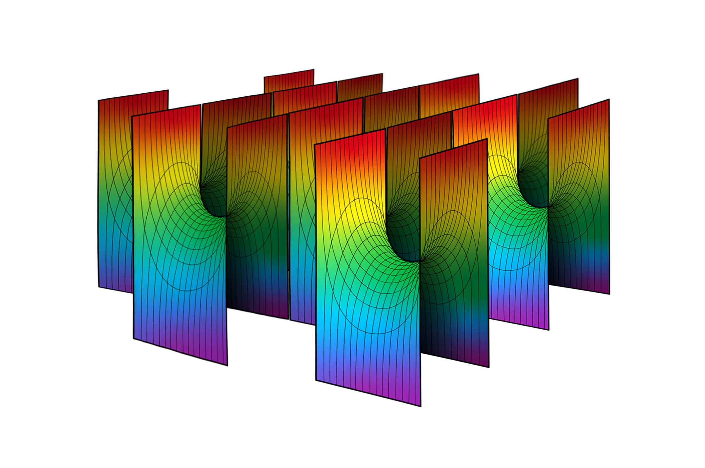
Figure 1: Scherk’s minimal surface.

This surface arises from the following quartic curve in the complex projective plane $\mathbb{P}^{2}$:

$$xy(x^{2}+y^{2}+z^{2})\,\,=\,\,0.$$ (2)

We use $X,Y,Z$ as affine coordinates for $\mathbb{R}^{3}$ and $x,y,z$ as homogeneous coordinates for $\mathbb{P}^{2}$. Scherk’s minimal surface is obtained as the Minkowski sum of two parametric space curves:

$$\begin{matrix}\!(X,Y,Z)\,\,&\,=&\bigl{(}{\rm arctan}(s),0,{\rm log}(s)-{\rm log}(s^{2}{+}1)/2\bigr{)}\\ &&+\,\,\bigl{(}0,-{\rm arctan}(t),-{\rm log}(t)+{\rm log}(t^{2}{+}1)/2\bigr{)}.\end{matrix}$$ (3)

The derivation of (1) from (2) via (3) is given in Example 1. This computation is originally due to Richard Kummer (Kum, , p. 52) whose 1894 dissertation also displays a plaster model.

Following the classical literature (cf. Little83 ; Sch ), a surface of double translation equals

$$\mathcal{S}\quad=\quad\mathcal{C}_{1}+\mathcal{C}_{2}\,\,=\,\,\mathcal{C}_{3}+\mathcal{C}_{4},$$

where $\mathcal{C}_{1},\mathcal{C}_{2},\mathcal{C}_{3},\mathcal{C}_{4}$ are curves in $\mathbb{R}^{3}$, and the two decompositions are distinct.

We note that Scherk’s minimal surface (1) is a surface of double translation. A first representation $\mathcal{S}=\mathcal{C}_{1}+\mathcal{C}_{2}$ was given in (3). A second representation $\mathcal{S}=\mathcal{C}_{3}+\mathcal{C}_{4}$ equals

$$\begin{matrix}X&=&{\rm arctan}(u)\,\,\,+\,\,\,{\rm arctan}(v)&=&{\rm arctan}\bigl{(}\frac{u+v}{1-uv}\bigr{)},\vskip 6.0pt plus 2.0pt minus 2.0pt\\ Y&=&{\rm arctan}(5u)\,\,+\,\,{\rm arctan}(5v)&=&\,{\rm arctan}\bigl{(}\frac{5u+5v}{1-25uv}\bigr{)},\vskip 3.0pt plus 1.0pt minus 1.0pt\\ Z&=&\frac{1}{2}{\rm log}\bigl{(}\frac{1+(5u)^{2}}{5(1+u^{2})}\bigr{)}\,+\,\frac{1}{2}{\rm log}\bigl{(}\frac{1+(5v)^{2}}{5(1+v^{2})}\bigr{)}.&&\end{matrix}$$ (4)

It is instructive to verify that both parametrizations (3) and (4) satisfy the equation (1).

A remarkable theorem due to Sophus Lie LieGes2 , refined by Henri Poincaré in Poin95 , states that these are precisely the surfaces derived from plane quartic curves by the integrals appearing in Abel’s Theorem. The implicit equation of such a surface is an analytic object introduced by Bernhard Riemann. Namely, if the quartic is smooth then this is Riemann’s theta function $\theta$. Modern algebraic geometers view the surface $\{\theta=0\}$ as the theta divisor in the Jacobian. We replace that abelian threefold by its universal cover $\mathbb{C}^{3}$ and we focus on the subset $\mathbb{R}^{3}$ of real points. Our object of study is the real analytic surface $\{\theta=0\}$ in $\mathbb{R}^{3}$.

The present article is organized as follows. Section 2 derives the parametrization of theta surfaces by abelian integrals. We review Abel’s Theorem 2.1, Riemann’s Theorem 2.2 and Lie’s Theorem 2.3, all from the perspective developed by Lie’s successors in Eies08 ; Eies09 ; Kum ; Sch ; Wie . In Section 3 we present a symbolic algorithm for computing theta surfaces. Here the input is a reducible quartic curve whose abelian integrals can be evaluated in closed form in a computer algebra system. As an illustration we show how (3) and (1) are derived from (2).

In Section 4 we discuss degenerations of curves and their Jacobians via tropical geometry. This leads to the formula in Theorem 4.1 for the implicit equation of a degenerate theta surface. Based on the combinatorics of Voronoi cells and Delaunay polytopes, this offers a present-day explanation for formulas, such as (1), that were found well over a century ago.

Theta surfaces are usually transcendental, but they can be algebraic in special situations. Algebraic theta surfaces were classified by John Eiesland in Eies08 . Examples include the cubic surface mentioned by Shiing-Shen Chern in (Chern, , p. 2), the quintic surface shown by John Little in (Little83, , Example 4.3) and the quadric surface arising from the union of four concurrent lines in Example 8. In Section 5 we revisit Eiesland’s census of quartics with algebraic theta surfaces. We present derivations and connections to sigma functions BEL ; naka .

In Section 6 we study theta surfaces via numerical computation. Building on state-of-the-art methods for evaluating abelian integrals and theta functions, we develop a numerical algorithm whose input is a smooth quartic curve in $\mathbb{P}^{2}$ and whose output is its theta surface.

Our article proposes the name theta surface for what Sophie Lie called a surface of double translation. We return to historical sources in Section 7, by offering a retrospective on the remarkable work done in Leipzig in the late $19$th century by Lie’s circle Lie ; Sch . Our presentation here serves to connect differential geometry and algebraic geometry, reconciling the $19$th and $20$th centuries, with a view towards applied mathematics in the $21$st century. On that note, there is a natural connection to integrable systems and mathematical physics. The three-phase solutions DFS to the KP equation are closely related to theta surfaces. Double translation surfaces also represent invariants in the study of 4-wave interactions in BalFer .

2 Parametrization by Abelian Integrals

We begin with the parametric representation of theta surfaces. Our point of departure is a real algebraic curve $\mathcal{Q}$ of degree four in the projective plane $\mathbb{P}^{2}$. This is the zero set of a ternary quartic that is unique up to scaling. We thus identify the curve with its polynomial

$$\qquad Q(x,y,z)\quad=\,\,\sum_{i+j+k=4}\!\!c_{ijk}x^{i}y^{j}z^{k},\qquad\qquad c_{ijk}\in\mathbb{R}.$$

This quartic can be reducible, as in (2), but we assume that it is squarefree. The symbol $\mathcal{Q}$ refers to the complex curve, and we write $\mathcal{Q}_{\mathbb{R}}$ for its subset of real points. If $\mathcal{Q}$ is nonsingular then it is a non-hyperelliptic Riemann surface of genus $3$, canonically embedded into $\mathbb{P}^{2}$.

The holomorphic differentials on $\mathcal{Q}$ comprise a $3$-dimensional vector space $H^{0}(\mathcal{Q},\Omega^{1}_{\mathcal{Q}})$. Assuming that $z$ does not divide $Q$, we choose a basis $\{\omega_{1},\omega_{2},\omega_{3}\}$ for this space as follows. Consider the dehomogenization $q(x,y)=Q(x,y,1)$, set $q_{x}=\partial q/\partial x$ and $q_{y}=\partial q/\partial y$, and fix

$$\omega_{1}\,=\,\frac{x}{q_{y}}dx\,,\quad\omega_{2}\,=\,\frac{y}{q_{y}}dx\,,\quad\omega_{3}\,=\,\frac{1}{q_{y}}dx.$$ (5)

As the quartic $q(x,y)$ is defined over $\mathbb{R}$, so is the basis. To be precise, all coefficients appearing in the $\omega_{i}$ are real numbers. Since $\,dq=q_{x}dx+q_{y}dy=0\,$ holds on $\mathcal{Q}$, we can also write

$$\omega_{1}\,=\,-\frac{x}{q_{x}}dy\,,\quad\omega_{2}\,=\,-\frac{y}{q_{x}}dy\,,\quad\omega_{3}\,=\,-\frac{1}{q_{x}}dy.$$ (6)

Remark 1

If $p=(x:y:1)$ is any point on $\mathcal{Q}$, then $\,(\omega_{1}(p):\omega_{2}(p):\omega_{3}(p))\,=\,p$. This reflects the fact that $\mathcal{Q}$ is the canonical embedding of the abstract curve underlying $\mathcal{Q}$.

Consider a path on the Riemann surface $\mathcal{Q}$ with end points $p$ and $r$. We can integrate the form $\omega_{i}$ along that path and obtain a complex number $\int_{p}^{r}\omega_{i}$. If the path is real, from $p$ to $r$ on a single connected component of the real curve $\mathcal{Q}_{\mathbb{R}}$, then $\int_{p}^{r}\omega_{i}$ is a real number. This number is computed in practise by regarding $y=y(x)$ as a function of $x$, defined by $q(x,y)=0$, and by computing the definite integral from the $x$-coordinate of $p$ to the $x$-coordinate of $r$. Alternatively, after replacing (5) with (6), we can regard $x=x(y)$ as an implicitly defined function of $y$, and take the definite integral from the $y$-coordinate of $p$ to that of $r$.

We fix a line $\mathcal{L}(0)$ in $\mathbb{P}^{2}$ that intersects $\mathcal{Q}$ in four distinct nonsingular points $p_{1}(0)$, $p_{2}(0),p_{3}(0)$ and $p_{4}(0)$. For $p_{j}\in\mathcal{Q}$ sufficiently close to $p_{j}(0)$, we obtain an analytic curve

$$\begin{matrix}\Omega_{j}(p_{j})\,\,=\,\,(\Omega_{1j},\Omega_{2j},\Omega_{3j})(p_{j})\,\,=\,\,\bigl{(}\,\int_{p_{j}(0)}^{p_{j}}\omega_{1}\,,\,\int_{p_{j}(0)}^{p_{j}}\omega_{2}\,,\,\int_{p_{j}(0)}^{p_{j}}\omega_{3}\,\bigr{)}.\end{matrix}$$ (7)

Remark 2

By the Fundamental Theorem of Calculus, the derivatives of these curves are

$$\dot{\Omega}_{j}(p_{j})\,\,\,=\,\,\,(\omega_{1}(p_{j}),\omega_{2}(p_{j}),\omega_{3}(p_{j}))\,\,\,=\,\,\,p_{j}.$$

Here, the derivative is performed with respect to the local parameter of the point $p_{j}$. The second equality is Remark 1. In words, the tangent direction to $\Omega_{j}$ at $p_{j}$ is $p_{j}$ itself.

The following theorem paraphrases a basic result from the theory of Riemann surfaces:

Theorem 2.1 (Abel’s Theorem)

Suppose that the points $p_{1},p_{2},p_{3},p_{4}$ are collinear. Then

$$\Omega_{1}(p_{1})\,+\,\Omega_{2}(p_{2})\,+\,\Omega_{3}(p_{3})\,+\,\Omega_{4}(p_{4})\,\,\,=\,\,\,0.$$

Now, let us fix analytic coordinates $s,t$ on the curve, centered at $p_{1}(0)$ and $p_{2}(0)$ respectively. Then, for every choice of $s,t$ in a small neighborhood of $0$, we obtain two nearby points $p_{1}(s),p_{2}(t)$. The corresponding theta surface $\mathcal{S}$ is the image of the parametrization

$$(s,t)\quad\mapsto\quad\Omega_{1}(p_{1}(s))\,+\,\Omega_{2}(p_{2}(t)).$$ (8)

The image is a complex analytic surface $\mathcal{S}$ in $\mathbb{C}^{3}$. However, if the points $p_{1}(0)$ and $p_{2}(0)$ are real then we take $s$ and $t$ in a small neighborhood of $0$ in $\mathbb{R}$, and $\mathcal{S}$ is a real surface in $\mathbb{R}^{3}$. This surface is analytic and only defined locally, since $s$ and $t$ are local parameters.

Shifting gears, let us now consider an arbitrary analytic surface $\mathcal{T}$ in $\mathbb{C}^{3}$. We say that $\mathcal{T}$ is a translation surface if there are two smooth analytic curves $\mathcal{C}_{1},\mathcal{C}_{2}\subset\mathbb{C}^{3}$ such that

$$\mathcal{T}\,\,=\,\,\mathcal{C}_{1}\,+\,\mathcal{C}_{2}\,\,=\,\,\bigl{\{}\,p_{1}+p_{2}\,\,|\,\,p_{1}\in\mathcal{C}_{1},p_{2}\in\mathcal{C}_{2}\,\bigr{\}}.$$

In words, $\mathcal{T}$ is the Minkowski sum of the two generating curves $\mathcal{C}_{1}$ and $\mathcal{C}_{2}$. We require the parametrization to be injective, i.e. for each point $x\in\mathcal{T}$ there are unique points $p_{1}\in\mathcal{C}_{1},p_{2}\in\mathcal{C}_{2}$ such that $x=p_{1}+p_{2}$. Note that, if $\alpha_{1},\alpha_{2}\colon\Delta\to\mathbb{C}^{3}$ are local parametrizations of the generating curves $\mathcal{C}_{1},\mathcal{C}_{2}$, then the translation surface $S$ has the parametrization

$$\mathcal{T}\,\,=\,\,\{\alpha_{1}(s)+\alpha_{2}(t)\}\,\,=\,\,\left\{\begin{pmatrix}\alpha_{11}(s)+\alpha_{21}(t)\\ \alpha_{12}(s)+\alpha_{22}(t)\\ \alpha_{13}(s)+\alpha_{23}(t)\end{pmatrix}\right\}.$$

Definition 1 (Double translation surfaces)

A translation surface $\mathcal{T}\subset\mathbb{C}^{3}$ as above is a double translation surface if there exists other smooth analytic curves $\mathcal{C}_{3},\mathcal{C}_{4}\subset\mathbb{C}^{3}$ such that

$$\mathcal{T}\,\,=\,\,\mathcal{C}_{1}\,+\,\mathcal{C}_{2}\,\,=\,\,\mathcal{C}_{3}\,+\,\mathcal{C}_{4}.$$ (9)

Returning to the setting of algebraic geometry, let $\mathcal{S}$ be the theta surface derived as above from a quartic curve $\mathcal{Q}$ in the plane $\mathbb{P}^{2}$. This formula (8) shows that $\mathcal{S}$ is a translation surface. In fact, the theta surface $\mathcal{S}$ is a double translation surface. This is a consequence of Abel’s Theorem. To see this, consider the line $\mathcal{L}$ that is spanned by the points $p_{1}(s)$ and $p_{2}(t)$ in $\mathbb{P}^{2}$. This line intersects the quartic curve $\mathcal{Q}$ in two other points $p_{3}(s,t)$ and $p_{4}(s,t)$, and these points are close to $p_{3}(0)$ and $p_{4}(0)$ respectively. Theorem 2.1 says that

$$\Omega_{1}(p_{1}(s))\,+\,\Omega_{2}(p_{2}(t))\,\,=\,\,-\Omega_{3}(p_{3}(s,t))\,-\,\Omega_{4}(p_{4}(s,t)).$$ (10)

The points $p_{3}(s,t)$ and $p_{4}(s,t)$ span the same line $\mathcal{L}$, so they determine $p_{1}(s)$ and $p_{2}(t)$ as the residual intersection points of the curve $\mathcal{Q}$ with $\mathcal{L}$. This means that the points $p_{3}(s,t)$ and $p_{4}(s,t)$ can move freely in neighborhoods of $p_{3}(0)$ and $p_{4}(0)$ on the curve $\mathcal{Q}$. If $u,v$ are analytic coordinates on $\mathcal{Q}$, centered in $p_{3}(0)$ and $p_{4}(0)$ respectively, then (10) shows that

$$(u,v)\quad\mapsto\quad-\Omega_{3}(p_{3}(u))-\Omega_{4}(p_{4}(v))$$

is another parametrization of the surface $\mathcal{S}$. Hence (9) holds, with generating curves

$$\mathcal{C}_{1}=\Omega_{1}(p_{1}(s)),\quad\mathcal{C}_{2}=\Omega_{2}(p_{2}(t)),\qquad\mathcal{C}_{3}=-\Omega_{3}(p_{3}(u)),\quad\mathcal{C}_{4}=-\Omega_{4}(p_{4}(v)).$$ (11)

In particular, we see that the two translation structures on the theta surface $\mathcal{S}$ are distinct. Indeed, Remark 2 tells us that the tangent lines to these curves at $0$ correspond to the four points $p_{1}(0),p_{2}(0),p_{3}(0),p_{4}(0)\in\mathbb{P}^{2}$, and these are distinct by construction.

Remark 3

Remark 2 shows that the tangent directions to the analytic curves in (11) are

$$\dot{\mathcal{C}}_{1}(s) =\phantom{-}\dot{\Omega}_{1}(p_{1}(s))=p_{1}(s), \dot{\mathcal{C}}_{2}(t) =\phantom{-}\dot{\Omega}_{2}(p_{2}(t))=p_{2}(t),$$

$$\dot{\mathcal{C}}_{3}(u) =-\dot{\Omega}_{3}(p_{3}(u))=p_{3}(u), \dot{\mathcal{C}}_{4}(v) =-\dot{\Omega}_{4}(p_{4}(v))=p_{4}(v).$$

Here $p_{1}(s),p_{2}(t),p_{3}(u),p_{4}(v)$ are regarded as points in the projective plane $\mathbb{P}^{2}$, indicating tangent directions in $\mathbb{C}^{3}$, so the sign does not matter. Hence, as in Remark 1, the analytic arcs $\dot{\mathcal{C}}_{1},\dot{\mathcal{C}}_{2},\dot{\mathcal{C}}_{3},\dot{\mathcal{C}}_{4}$ lie on the quartic $\mathcal{Q}$. In particular, if we are given a theta surface $\mathcal{S}$ and one generating curve $\mathcal{C}_{i}$, but not the quartic $\mathcal{Q}$, then we can recover $\mathcal{Q}$ as a quartic in $\mathbb{P}^{2}$ that contains the analytic arc $\dot{\mathcal{C}}_{i}$. This fact will be used in Section 7, together with a result of Lie, to give a differential-geometric solution to Torelli’s problem for genus three curves.

Now assume that $\mathcal{Q}$ is a smooth quartic curve. Then we can find an implicit equation for our surface via the Riemann theta function. Recall Fay ; Mum1 that this is the holomorphic function

$$\theta(\mathbf{x},B)\,\,=\,\,\sum_{n\in\mathbb{Z}^{3}}\mathbf{e}\left(-\frac{1}{2}n^{t}Bn\,+\,i\,n^{t}\mathbf{x}\right)\,\,=\,\,\sum_{n\in\mathbb{Z}^{3}}\exp\left(-\pi n^{t}Bn\right)\cdot\operatorname{cos}(2\pi n^{t}\mathbf{x}),$$ (12)

where $\mathbf{e}(t):=\exp(2\pi t)$, $\mathbf{x}=(X,Y,Z)\in\mathbb{C}^{3}$, and $B\in\mathbb{C}^{3\times 3}$ is a symmetric matrix with positive-definite real part. The second sum shows that $\theta$ takes real values if $B$ and $\mathbf{x}$ are real.

This definition is slightly different from the usual ones, where $B$ is taken either with positive definite imaginary part or with negative definite real part. We choose this version of the Riemann theta function in order to highlight the real numbers. Namely, the theta divisor

$$\Theta_{B}\,\,:=\,\,\{\,\mathbf{x}\,\,|\,\,\theta(\mathbf{x},B)=0\,\}\,\,\,\subset\,\,\,\mathbb{C}^{3}.$$ (13)

restricts to a real analytic surface when both $\mathbf{x}$ and $B$ are real. In general, we will show that the theta divisor coincides with the theta surface above. To this end, we choose a symplectic basis $\alpha_{1},\beta_{1},\alpha_{2},\beta_{2},\alpha_{3},\beta_{3}$ for $H_{1}(\mathcal{Q},\mathbb{Z})$. The intersection product on $\mathcal{Q}$ is given by

$$(\alpha_{j}\cdot\alpha_{k})=0,\qquad(\beta_{j}\cdot\beta_{k})=0,\quad{\rm and}\quad(\alpha_{j}\cdot\beta_{k})=\delta_{jk}.$$

The period matrix for the Riemann surface $\mathcal{Q}$ with respect to this basis equals

$$\Pi\,\,=\,\,\left(\Pi_{\alpha}\,|\,\Pi_{\beta}\right)\,\,\in\,\,\mathbb{C}^{3\times 6},$$ (14)

with entries $(\Pi_{\alpha})_{jk}=\int_{\alpha_{k}}\omega_{j}$ and $(\Pi_{\beta})_{jk}=\int_{\beta_{k}}\omega_{j}$. As a consequence of Riemann’s relations (Mum1, , Theorem 2.1), the matrix $\Pi_{\alpha}$ is invertible, and the corresponding Riemann matrix is

$$B\,\,=\,\,-i\cdot\Pi_{\alpha}^{-1}\Pi_{\beta}.$$ (15)

Riemann’s relations also show that the matrix $B$ is symmetric with positive-definite real part, so we can consider the theta divisor $\,\Theta_{B}\subset\mathbb{C}^{3}\,$ as in (13). A fundamental theorem of Riemann implies that this coincides with our theta surface, up to a change of coordinates.

Theorem 2.2 (Riemann’s Theorem)

The theta surface $\mathcal{S}$ and the theta divisor $\Theta_{B}$ coincide up to an affine change of coordinates on $\mathbb{C}^{3}$. More precisely, there is a vector $c\in\mathbb{C}^{3}$ such that

$$\mathcal{S}\,\,=\,\,\Pi_{\alpha}\cdot\Theta_{B}+c,$$ (16)

where the equality is meant on all points where the parametrized surface $\mathcal{S}$ is defined.

Proof

We outline how to obtain this result from the usual statement of Riemann’s Theorem. Let $(\eta_{1},\eta_{2},\eta_{3})$ be the basis of $H^{0}(\mathcal{Q},\Omega^{1}_{\mathcal{Q}})$ obtained from $(\omega_{1},\omega_{2},\omega_{3})$ by coordinate change with the matrix $\Pi_{\alpha}^{-1}$. Then $\int_{\alpha_{j}}\eta_{k}=\delta_{kj}$ and $\int_{\beta_{j}}\eta_{k}=i\cdot B_{kj}$. Fix a point $r\in\mathcal{Q}$, paths from $r$ to $p_{1}(0)$ and from $r$ to $p_{2}(0)$, and local coordinates $s,t$ on $\mathcal{Q}$ around $p_{1}(0)$ and $p_{2}(0)$. For $s,t$ small, we consider paths from $r$ to $p_{1}(s)$ and from $r$ to $p_{2}(t)$. This gives an analytic map

$$(s,t)\,\,\,\mapsto\,\,\,\begin{pmatrix}\int_{r}^{p_{1}(s)}\eta_{1}\\ \int_{r}^{p_{1}(s)}\eta_{2}\\ \int_{r}^{p_{1}(s)}\eta_{3}\end{pmatrix}\,+\,\begin{pmatrix}\int_{r}^{p_{2}(t)}\eta_{1}\\ \int_{r}^{p_{2}(t)}\eta_{2}\\ \int_{r}^{p_{2}(t)}\eta_{3}\end{pmatrix}.$$

The familiar form of Riemann’s theorem (Mum1, , Theorem 3.1) shows that there is a constant $\kappa\in\mathbb{C}^{3}$ such that the image of this map coincides with $\Theta_{B}-\kappa$. Now, it is enough to write

$$\int_{r}^{p_{1}(s)}\!\!\!\eta_{j}\,\,=\,\,\int_{r}^{p_{1}(0)}\!\!\!\eta_{j}\,\,+\,\,\int_{p_{1}(0)}^{p_{1}(s)}\!\!\!\eta_{j}\qquad{\rm and}\qquad\int_{r}^{p_{2}(t)}\!\!\!\eta_{j}\,\,=\,\,\int_{r}^{p_{2}(0)}\!\!\!\eta_{j}\,\,+\,\,\int_{p_{2}(0)}^{p_{2}(t)}\!\!\!\eta_{j},$$

and then change the coordinates from the basis $(\eta_{1},\eta_{2},\eta_{3})$ back to the basis $(\omega_{1},\omega_{2},\omega_{3})$.

Our discussion shows that each theta surface is also a surface of double translation, and the Riemann theta function provides an implicit equation when the quartic $\mathcal{Q}$ is smooth. A fundamental result of Lie states that all nondegenerate surfaces of double translation whose two parametrizations are distinct arise in this way. Here nondegenerate and distinct are technical conditions. The precise definition, phrased in modern language, can be found in (Little83, , Definition 2.2). In particular, the nondegeneracy hypothesis assures that none of the generating curves can be a line. This rules out special surfaces such as cylinders or planes.

We recall briefly Lie’s construction. Let $\mathcal{S}=\mathcal{C}_{1}+\mathcal{C}_{2}=\mathcal{C}_{3}+\mathcal{C}_{4}$ be any surface of double translation in $\mathbb{C}^{3}$. Then we can identify the tangent lines to the curves $\mathcal{C}_{j}$ with points in $\mathbb{P}^{2}$, and taking all these tangent lines we obtain analytic arcs $\dot{\mathcal{C}}_{1},\dot{\mathcal{C}}_{2},\dot{\mathcal{C}}_{3},\dot{\mathcal{C}}_{4}\subset\mathbb{P}^{2}$. If $\mathcal{S}$ is a theta surface then, by Remark 3, all these arcs lie on a common quartic curve $\mathcal{Q}$. Lie proved that this property holds for all nondegenerate surfaces of double translation $\mathcal{S}$.

Theorem 2.3 (Lie’s Theorem)

The arcs $\,\dot{\mathcal{C}}_{1},\dot{\mathcal{C}}_{2},\dot{\mathcal{C}}_{3},\dot{\mathcal{C}}_{4}\,$ lie on a common reduced quartic curve $\mathcal{Q}$ in the projective plane $\mathbb{P}^{2}$, and $\mathcal{S}$ coincides with the theta surface associated to $\mathcal{Q}$.

Lie’s original proof Lie involves a complicated system of differential equations satisfied by the parametrizations of the curves $\mathcal{C}_{j}$. These differential equations force the arcs $\dot{\mathcal{C}}_{j}$ to lie on a quartic. A much simpler proof was subsequently given by Darboux Darb . A modern exposition is found in Little’s paper Little83 , together with generalizations to higher dimensions.

3 Symbolic Computations for Special Quartics

There is a fundamental dichotomy in the study of theta surfaces, depending on the nature of the underlying quartic in $\mathbb{P}^{2}$. If it is a smooth quartic then Riemann’s Theorem 2.2 furnishes the defining equation of the theta surface. This is the case to be studied numerically in Section 6. At the other end of the spectrum are the singular quartics considered in the classical literature. Here methods from computer algebra can be used to compute the theta surface. This is our topic in the current section. Our focus lies on evaluating the abelian integrals in (7) by exact symbolic computations, as opposed to numerical evaluations of the integrals.

We begin by explaining these methods for our running example from the Introduction.

Example 1 (Scherk’s minimal surface)

We here derive (3) from (2). This serves as a first illustration for Algorithm 1 below. We start with the quartic $q(x,y)=xy(x^{2}+y^{2}+1)$. This is the dehomogenization of (2) with respect to $z$. Using the partial derivatives $q_{y}(x,y)=x^{3}+3xy^{2}+x$ and $q_{x}(x,y)=3x^{2}y+y^{3}+y$, we compute the differential forms in (5) and (6).

We choose to evaluate the integrals in (7) over the lines $y=0$ and $x=0$. These will give us the two summands in the parametrization (8). The first summand is obtained by setting $x=s$ and $y=0$, so that $q_{y}(s,0)=s(s^{2}+1)$, and by computing the antiderivatives of the resulting specialized forms $\omega_{j}(s,0)$ for $j=1,2,3$. The three coordinates of $\Omega_{1}(p_{1}(s))$ are

$$\begin{matrix}\Omega_{11}(p_{1}(s))&=&\int\frac{s}{s(s^{2}+1)}ds&=&\arctan(s),\vskip 3.0pt plus 1.0pt minus 1.0pt\\ \Omega_{21}(p_{1}(s))&=&\int\frac{0}{s(s^{2}+1)}ds&=&0,\vskip 3.0pt plus 1.0pt minus 1.0pt\\ \Omega_{31}(p_{1}(s))&=&\int\frac{1}{s(s^{2}+1)}ds&=&\log(s)-\frac{1}{2}\log(s^{2}+1).\end{matrix}$$

The second summand is obtained by integrating over the line $x=0$, with parameter $y=t$, so that $q_{x}(0,t)=t(t^{2}+1)$ in (6). The three coordinates of $\Omega_{2}(p_{2}(t))$ are found to be

$$\begin{matrix}\Omega_{12}(p_{2}(t))&=&-\int\frac{0}{t(t^{2}+1)}dt&=&0,\vskip 3.0pt plus 1.0pt minus 1.0pt\\ \Omega_{22}(p_{2}(t))&=&-\int\frac{t}{t(t^{2}+1)}dt&=&-\arctan(t),\vskip 3.0pt plus 1.0pt minus 1.0pt\\ \Omega_{32}(p_{2}(t))&=&-\int\frac{1}{t(t^{2}+1)}dt&=&-\log(t)+\frac{1}{2}\log(t^{2}+1).\end{matrix}$$

By adding these integrals, we obtain the parametrization of the corresponding theta surface:

$$X\,=\,\arctan(s)\,,\quad Y\,=\,-\arctan(t)\,,\quad Z\,=\,\log\Big{(}\frac{s}{\sqrt{s^{2}+1}}\Big{)}-\log\Big{(}\frac{t}{\sqrt{t^{2}+1}}\Big{)}.$$ (17)

This is Scherk’s minimal surface (3). Trigonometry now yields the implicit equation in (1).

The following algorithm summarizes the steps we have performed in Example 1. Starting from the quartic curve in $\mathbb{P}^{2}$, we compute the two generating curves of the associated theta surface in $\mathbb{C}^{3}$. This is done by evaluating the integrals in (7) as explicitly as possible.

Input: A quartic equation $q(x,y)$ describing a reduced plane quartic curve.

Output: The parametrization (8) of the theta surface $\mathcal{S}$ in affine $3$-space.

Step 1: Specify two points $p_{1}$ and $p_{2}$ on the quartic.

Step 2: Fix local parameters $(x_{1},y_{1})$ and $(x_{2},y_{2})$ around $p_{1}$ and $p_{2}$ respectively.

Step 3: Write $y_{j}$ as an algebraic function in $x_{j}$ on its branch.

Step 4: Compute the partial derivative $q_{y}$ on the two branches.

Step 5: Substitute $x_{1}=s$ and $x_{2}=t$ into the differential forms $\omega_{1},\omega_{2},\omega_{3}$ in (5).

Step 6: By integrating these differential forms, compute the vectors

$$\begin{matrix}\Omega_{1}(p_{1}(s))&=&(\int\frac{s}{q_{y}(s,y_{1}(s))}ds,\int\frac{y_{1}(s)}{q_{y}(s,y_{1}(s))}ds,\int\frac{1}{q_{y}(s,y_{1}(s))}ds),\\ \Omega_{2}(p_{2}(t))&=&(\int\frac{t}{q_{y}(t,y_{2}(t))}dt,\int\frac{y_{2}(t)}{q_{y}(t,y_{2}(t))}dt,\int\frac{1}{q_{y}(t,y_{2}(t))}dt).\end{matrix}$$

Step 7: Output the sum $\Omega_{1}(p_{1}(s))+\Omega_{2}(p_{2}(t))$ of the generating curves as in (8).

Algorithm 1 Computing the parametrized theta surface from its plane quartic

One important part of Algorithm 1 is Step 3, where $y_{j}$ is represented as an algebraic function in $x_{j}$. This function has algebraic degree at most four, so it can be written in radicals. After all, the steps above are meant as a symbolic algorithm. However, we found the representation in radicals to be infeasible for practical computations unless the quartic is very special. Even more crucial is the computation of the indefinite integrals in Step 6. This can be done explicitly whenever the quartic is reducible and all the components are rational: in that special case, the holomorphic differentials of (5) restrict to a differential $\frac{f(t)}{g(t)}dt$ on $\mathbb{P}^{1}$ where $f(t),g(t)$ are polynomials, and any such expression can be integrated symbolically.

In what follows we focus on instances where the quartic $q(x,y)$ is reducible. A reducible plane quartic is one of the followings: four straight lines, a conic and two straight lines, two conics, or a cubic and a line. In the sequel, we show the computations of such theta surfaces using Algorithm 1. The first three cases were worked out by Richard Kummer Kum in his thesis, and the latter case was studied by Georg Wiegner Wie . We here present three further examples of non-algebraic theta surfaces. The algebraic ones will be discussed in Section 5.

Consider the first three of the four cases above. Then $q(x,y)$ factors into two conics. The two conics meet in four points in $\mathbb{P}^{2}$. We consider the pencil of conics through these points.

Remark 4

A result due to Lie states that the theta surface $\mathcal{S}$ for a product of two conics only depends on their pencil, provided $p_{1}$ and $p_{2}$ lie on the same conic (cf. (Kum, , Section 3)). Hence $\mathcal{S}$ has infinitely many distinct representations $\mathcal{C}_{1}+\mathcal{C}_{2}$ as a translation surface. We shall return to this topic in Theorem 7.2, where it is shown how to compute these representations.

For instance, for Scherk’s surface in Example 1, the four points in $\mathbb{P}^{2}$ are $(i:0:1),(-i:0:1),(0:i:1),(0:-i:1)$, and the pencil is generated by $xy$ and $x^{2}+y^{2}+z^{2}$. We can replace these two quadrics by any other pair in the pencil and obtain two generating curves.

We now examine another case which is similar. It will lead to the theta surface in (20).

Example 2

Fix the four points $(1:0:0),(0:1:0),(0:0:1),(1:1:1)$ in $\mathbb{P}^{2}$. Their pencil of conics is generated by $y(x-z)$ and $(x-y)z$. We multiply the first conic with a general member of the pencil to get the quartic $Q=y(x-z)\cdot((1+\lambda)xy-xz-\lambda yz)$. Here $\lambda$ is a parameter, which we included in order to illustrate Remark 4. Dehomogenizing $Q$, we get $q=y(x-1)((1+\lambda)xy-x-\lambda y)$. We compute $\omega_{1},\omega_{2},\omega_{3}$ from the partial derivatives

$$q_{x}\,=\,y((1+\lambda)xy-x-\lambda y)+y(x-1)((1+\lambda)y-1)),$$

$$q_{y}\,=\,(x-1)((1+\lambda)xy-x-\lambda y)+y(x-1)((1+\lambda)x-\lambda).$$

We integrate over the two lines given by $y(x-1)=0$. On the first line $\{y=0\}$, we have $q_{y}=-x(x-1)$. The indefinite forms of the three abelian integrals in $\Omega_{1}(p_{1}(s))$ are

$$\begin{matrix}\int\frac{s}{-s(s-1)}ds\,=\,\log\left(\frac{1}{s-1}\right)\,,\quad\int\frac{0}{-s(s-1)}ds\,=\,0\,,\quad\int\frac{1}{-s(s-1)}ds\,=\,\log\bigl{(}\frac{s}{s-1}\bigr{)}.\end{matrix}$$

For the line $\{x-1=0\}$ we transform the differentials by passing from (5) to (6). We find

$$\begin{matrix}\int\frac{1}{-t(t-1)}dt=\log\bigl{(}\frac{t}{t-1}\bigr{)}\,,\quad\int\frac{t}{-t(t-1)}dt=\log\left(\frac{1}{t-1}\right)\,,\quad\int\frac{1}{-t(t-1)}dt=\log\bigl{(}\frac{t}{t-1}\bigr{)}.\end{matrix}$$

We conclude that the resulting theta surface has the parametric representation

$$\begin{matrix}&X&=&\log\left(\frac{1}{s-1}\right)\,+\,\log\bigl{(}\frac{t}{t-1}\bigr{)},\vskip 3.0pt plus 1.0pt minus 1.0pt\\ &Y&=&\qquad 0\,\,\,\,+\,\,\,\log\left(\frac{1}{t-1}\right),\vskip 3.0pt plus 1.0pt minus 1.0pt\\ &Z&=&\log\bigl{(}\frac{s}{s-1}\bigr{)}\,+\,\log\bigl{(}\frac{t}{t-1}\bigr{)}.\end{matrix}$$ (18)

Remark 5

The output of Algorithm 1 looks like (17) or (18). It gives the theta surface $\mathcal{S}$ in parametric form. Whenever the quartic is rational nodal, meaning that all the components are rational and with at most nodes as singularities, as in Figure 2, the expressions found for $X$, $Y$ and $Z$ are $\mathbb{C}$-linear combinations of logarithms of linear functions in $s$ and $t$. Indeed, since the singularities are nodal, the differentials of (5) restrict to each rational component $\Gamma\cong\mathbb{P}^{1}$ as meromorphic differentials with at most simple poles (ACG, , Chapter 2). Each such differential can be written as a sum of terms of the form $\frac{1}{(t-a)}$, which integrate to $\log(t-a)$.

From a representation as a $\mathbb{C}$-linear combination of logarithms we find an implicit equation for $\mathcal{S}$ by familiar elimination techniques from symbolic computation, such as resultants or Gröbner bases. Namely, we choose constants $\alpha,\beta,\gamma\in\mathbb{C}$ such that ${\rm exp}(\alpha X)$, ${\rm exp}(\beta Y)$ and ${\rm exp}(\gamma Z)$ are written as rational functions in $s$ and $t$, and we then eliminate $s$ and $t$ to obtain a trivariate polynomial $\Psi(u,v,w)$ such that $\mathcal{S}$ is defined locally by

$$\Psi\bigl{(}\,{\rm exp}(\alpha X),\,{\rm exp}(\beta Y),\,{\rm exp}(\gamma Z)\,\bigr{)}\,\,\,=\,\,\,0.$$ (19)

For the output (17), we take $\alpha=\beta=i$, $\,\gamma=1$ and $\,\Psi=uv^{2}w-u^{2}v-uw+v$. With these choices, (19) is precisely the implicit equation (1) of Scherk’s surface, times a constant.

For Example 2, the implicit equation is especially nice. The output (18) suggests the choices $\alpha=\beta=\gamma=1$ and $\,\Psi=u+v-w+1$, and hence the theta surface is given by

$${\rm exp}(X)\,+\,{\rm exp}(Y)\,-\,{\rm exp}(Z)\,\,=\,\,-1.$$ (20)

An explanation for the occurrence of such exponential sums is offered in Section 4.

We present two more illustrations of our methodology for special quartics. In each case we carry out both Algorithm 1 and the subsequent implicitization step as in Remark 5.

Example 3

Consider the quartic $q=xy(1-x^{2}+y^{2})$. This corresponds to the pencil of conics through $(0:i:1),(0:-i:1),(1:0:1),(-1:0:1)$. For the abelian integrals, we compute the partial derivatives $q_{x}=y(y^{2}-x^{2}+1)-2x^{2}y$ and $q_{y}=x(y^{2}-x^{2}+1)+2xy^{2}$.

We first integrate the differential forms in (6) over the line $y=0$, with local parameter $x=s$. On this component, $q_{x}=x(1-x^{2})$. The indefinite integrals are found to be

$$\begin{matrix}\!\int\!\!\frac{s}{-s(s^{2}-1)}ds=\frac{1}{2}\log(\frac{{s{+}1}}{{s{-}1}})),\quad\quad\int\!\!\frac{0}{-s(s^{2}-1)}ds=0,\quad\quad\int\!\!\frac{1}{-s(s^{2}-1)}ds=\log(s)-\!\frac{1}{2}\log(s^{2}{-}1).\end{matrix}$$

We next integrate over the line $x=0$, using (5) with $q_{y}=y(y^{2}+1)$. The abelian integrals are

$$\begin{matrix}\int\frac{0}{-t(1+t^{2})}dt\,=\,0\,,\quad\int\frac{t}{-t(1+t^{2})}dt\,=\,-\arctan(t)\,,\quad\int\frac{1}{-t(1+t^{2})}dt\,=\,-\log(t)\,+\,\frac{1}{2}\log(1+t^{2}).\end{matrix}$$

We conclude that the output of Step 7 in Algorithm 1 equals

$$X\,\,=\,\,\frac{1}{2}\log(s+1)-\frac{1}{2}\log(s-1),$$

$$Y\,\,=\,\,-\arctan(t)\,=\,-\frac{1}{2i}\log(t-i)+\frac{1}{2i}\log(t+i),$$

$$Z\,\,=\,\,\log(s)-\frac{1}{2}\log(s^{2}-1)-\log(t)+\frac{1}{2}\log(1+t^{2}).$$

From this we find that the implicit equation of the theta surface equals

$$-2\,{\rm exp}(Z)\,{\rm exp}(X)\,{\rm sin}(Y)\,-\,{\rm exp}(2X)\,-\,1=0.$$

Finding the two pairs of generating curves on a theta surface is particularly pleasant when the underlying quartic is the union of four lines in $\mathbb{P}^{2}$ that are defined over $\mathbb{Q}$.

Example 4

Consider the quartic $q=(y+x-1)(y-x-1)(y+x+1)(y-x+1)$. For the first pair of generating curves, we compute the abelian integrals over the first two lines:

$$\begin{matrix}\int\!\frac{1}{8(s-1)}ds\,=\,\frac{1}{8}\log(s-1),&\int\!-\frac{1}{8s}ds\,=\,-\frac{1}{8}\log(s),&\int\!\frac{1}{8s(s-1)}ds\,=\,\frac{1}{8}\log(s-1)-\frac{1}{8}\log(s),\\ \int\!\frac{1}{8(t+1)}dt\,=\,\frac{1}{8}\log(t+1),&\int\!\frac{1}{8t}dt=\frac{1}{8}\log(t),&\int\!\frac{1}{8t(t+1)}dt\,=\,-\frac{1}{8}\log(t+1)+\frac{1}{8}\log(t).\end{matrix}$$

Hence, the coordinates of the theta surface are given in terms of the parameters $s$ and $t$ by

$$8X\,\,=\,\,\log(s-1)+\log(t+1),$$

$$8Y\,\,=\,\,-\log(s)\,+\,\log(t),$$

$$8Z\,\,=\,\,\log(s-1)-\log(s)-\log(t+1)+\log(t).$$

Choosing $\alpha=\beta=\gamma=8$ in Remark 5, and hence $\,u={\rm exp}(8X),\,v={\rm exp}(8Y)$ and $w={\rm exp}(8Z)$, the implicit equation (19) of the theta surface is represented by the polynomial

$$\Psi(u,v,w)\,\,=\,\,u^{2}vw^{2}-2u^{2}vw-uv^{2}w+uvw^{2}+u^{2}v-4uvw-v^{2}w+uv-uw-2vw-w.$$

The same method works fairly automatically for any arrangement of four lines in the plane.

4 Degenerations of Theta Functions

We saw in Theorem 2.2 that the equation of the theta surface associated with a smooth plane quartic is a Riemann theta function. However, all theta surfaces seen in the classical literature were computed from quartics that are singular. In this section we explain how singularities induce degenerate theta functions. These are finite sums of exponentials, given combinatorially by the cells in the associated Delaunay subdivision of $\mathbb{Z}^{3}$. This furnishes a conceptual explanation of the equations defining theta surfaces like (1) or (20). Our approach is from the point of tropical geometry, which mirrors the theory of toroidal degenerations GruHu .

In what follows we focus on the rational nodal quartic curves. These are quartic curves whose irreducible components are rational. The special properties of such curves were already discussed briefly in Remark 5. Rational nodal quartics appear in five types: an irreducible quartic with three nodes, a nodal cubic together with a line, two smooth conics, a smooth conic with two lines, and an arrangement of four lines.

$\begin{array}[]{lllll}\includegraphics[width=56.9055pt]{nodalrationalquartic.pdf}&\includegraphics[width=56.9055pt]{nodalcubicline.pdf}&\includegraphics[width=56.9055pt]{twoconics.pdf}&\,\,\includegraphics[width=34.1433pt]{conictwolines.pdf}&\,\,\includegraphics[width=56.9055pt]{fourlines.pdf}\end{array}$

Figure 2: The five types of rational nodal quartics.

To each of these curves we associate its dual graph $\Gamma=(V,E)$. This has a vertex for each irreducible component and one edge for each intersection point between two components. A node on an irreducible component counts as an intersection of that component with itself.

$\begin{array}[]{lllll}\includegraphics[width=56.9055pt]{graph_nodalrationalquartic.pdf}&\includegraphics[width=56.9055pt]{graph_nodalcubicline.pdf}&\includegraphics[width=56.9055pt]{graph_twoconics.pdf}&\includegraphics[width=56.9055pt]{graph_conictwolines.pdf}&\includegraphics[width=56.9055pt]{graph_fourlines.pdf}\end{array}$

Figure 3: The dual graphs corresponding to the five types of rational nodal quartics.

The dual graphs play a key role in tropical geometry, namely in the tropicalization of curves and their Jacobians. We follow the combinatorial construction in (BBC, , Section 5). Fix one of the graphs $\Gamma$ in Figure 3 with an orientation for each edge. The first homology group

$$H_{1}(\Gamma,\mathbb{Z})\,\,=\,\,\ker\left(\partial\colon\mathbb{Z}^{E}\to\mathbb{Z}^{V}\right)$$

is free abelian of rank $3$. Let us fix a $\mathbb{Z}$-basis $\gamma_{1},\gamma_{2},\gamma_{3}$ for $H_{1}(\Gamma,\mathbb{Z})$. Each $\gamma_{j}$ is a directed cycle in $\Gamma$. We encode our basis in a $3\times|E|$ matrix $\Omega$. The entries in the $j$-th row of $\Omega$ are the coordinates of $\gamma_{j}$ with respect to the standard basis of $\mathbb{Z}^{E}$. Our five matrices $\Omega$ are

$$\!\begin{bmatrix}1&0&0\\ 0&1&0\\ 0&0&1\end{bmatrix}\!,\,\begin{bmatrix}1&\!\!\!-1&0&0\\ 0&1&\!\!-1&0\\ 0&0&0&1\end{bmatrix}\!,\,\begin{bmatrix}1&\!\!\!-1&0&0\\ 0&1&\!\!-1&0\\ 0&0&1&\!\!-1\end{bmatrix}\!,\,\begin{bmatrix}1&0&1&0&0\\ \!-1&1&0&\!\!-1&0\\ 0&\!\!\!-1&0&0&\!\!-1\end{bmatrix}\!,\,\begin{bmatrix}1&\!\!\!-1&0&1&0&0\\ \!-1&0&1&0&\!\!-1&0\\ 0&1&\!\!\!-1&0&0&1\end{bmatrix}\!.$$

We define the Riemann matrix of $\Gamma$ to be the positive definite symmetric $3\times 3$ matrix

$$B\,\,:=\,\,\Omega\cdot\Omega^{T}.$$ (21)

If we change the orientations and cycle bases then the matrix $B$ transforms under the action of ${\rm GL}(3,\mathbb{Z})$ by conjugation. The Riemann matrices of our five graphs are the matrices in the fourth column in Figure 4. The label  Form  refers to the quadratic form represented by $B$.

Figure 4: The Voronoi polytopes corresponding to the five types of rational nodal quartics, in reverse order to Figure 3. This diagram is taken from the dissertation of Frank Vallentin (Val, , Section 4.3, page 49). The first column gives the number $d$ of edges in the dual graph.

We now explain how a Riemann matrix $B$ of the dual graph as in (21) induces a degeneration to a singular curve with dual graph as in Figure 3. Let $B_{0}$ be a fixed (real or complex) symmetric $3\times 3$ matrix with positive definite real part. Consider the one-parameter family of classical Riemann matrices

$$B_{t}\,\,:=\,\,tB+B_{0}\qquad\text{for }\,\,t\geq 0.$$ (22)

We note that the real part of $B_{t}$ is always positive definite. If the chosen matrix $B_{0}$ does not belong to the hyperelliptic locus, then the set of positive real numbers $t$ such that $B_{t}$ lies on the hyperelliptic locus is discrete. Thus, almost all Riemann matrices $B_{t}$ correspond to non-hyperelliptic curves of genus three, and hence to smooth quartic curves in the plane.

We consider the Riemann theta functions for these curves. More precisely, we evaluate $\theta(\,\bullet\,,B_{t})$ at ${\bf x}$ translated by the vector $i\cdot tB\mathbf{a}$, where $\mathbf{a}=(a_{1},a_{2},a_{3})^{T}\in\mathbb{R}^{3}$. This gives

$$\begin{matrix}\theta\bigl{(}\mathbf{x}-i\cdot tB\mathbf{a},B_{t}\bigr{)}&=&\sum_{n\in\mathbb{Z}^{3}}\mathbf{e}\left(-\frac{1}{2}n^{T}(tB+B_{0})n+i\cdot n^{T}\left(\mathbf{x}-i\cdot tB\mathbf{a}\right)\right)\vskip 6.0pt plus 2.0pt minus 2.0pt\\ &=&\sum_{n\in\mathbb{Z}^{3}}\mathbf{e}\left(-\frac{1}{2}\left(n^{T}Bn-2n^{T}B\mathbf{a}\right)t-\frac{1}{2}n^{T}B_{0}n+i\cdot n^{T}\mathbf{x}\right)\vskip 6.0pt plus 2.0pt minus 2.0pt\\ &=&\sum_{n\in\mathbb{Z}^{3}}\mathbf{e}\left(-\frac{1}{2}(n^{T}Bn-2n^{T}B\mathbf{a})t\right)\cdot\mathbf{e}\left(-\frac{1}{2}n^{T}B_{0}n+i\cdot n^{T}\mathbf{x}\right).\end{matrix}$$

As $t\to+\infty$, the term $\mathbf{e}\left(-\frac{1}{2}(n^{T}Bn-2n^{T}B\mathbf{a})t\right)$ converges if and only if $\,n^{T}Bn-2n^{T}B\mathbf{a}\geq 0$. For each $n\in\mathbb{Z}^{3}$, this condition is a linear inequality in ${\bf a}$, which can be rewritten as follows:

$$\mathbf{a}^{T}B\mathbf{a}\,\,\,\leq\,\,(\mathbf{a}-n)^{T}B(\mathbf{a}-n).$$ (23)

Hence, in order for the theta function above to converge to a degenerate theta function, we must choose $\mathbf{a}$ in such a way that (23) is satisfied for every $n\in\mathbb{Z}^{3}$. The positive definite quadratic form given by $B$ defines a metric on $\mathbb{R}^{3}$. The condition (23) says that, among all lattice points $n$ in $\mathbb{Z}^{3}$, the origin is a closest one to $\mathbf{a}$ in this metric. This means that $\mathbf{a}$ is contained in the Voronoi cell with respect to the lattice $\mathbb{Z}^{3}$ and the metric defined by $B$.

The Voronoi cell is a $3$-dimensional polytope. It belongs to the class of unimodular zonotopes. The third column of Figure 4 shows this for each of the five types of nodal quartics in Figure 2. The translates of the Voronoi cell by vectors in $\mathbb{Z}^{3}$ define a tiling of $\mathbb{R}^{3}$. Their boundaries form an infinite $2$-dimensional polyhedral complex. See (BBC, , Figure 15) for the case of four lines, on the right in Figures 2 and 3. This surface is the tropical theta divisor in $\mathbb{R}^{3}$. It can be viewed as a polyhedral model for our degenerate theta surface. For details on these objects see BBC ; Chan and references therein. We encourage our readers to spot Figure 3 in (Chan, , Figures 1 and 8) and to examine the tropical Torelli map in (Chan, , Theorem 6.2).

We now assume that $\mathbf{a}$ is a vertex of the Voronoi cell. We write $\mathcal{D}_{{\bf a},B}$ for the set of all vectors $n\in\mathbb{Z}^{3}$ for which equality holds in (23). This set is finite for each Riemann matrix $B$ derived from a graph in Figure 3. We note the following behavior for the summands above:

$$\,\mathbf{e}\biggl{(}-\frac{1}{2}(n^{T}Bn-2n^{T}B\mathbf{a})t\biggr{)}\,\,\,\xrightarrow{t\rightarrow+\infty}\,\,\,\begin{cases}\,\,1&{\rm if}\,\,n\in\mathcal{D}_{{\bf a},B},\\ \,\,0&{\rm if}\,\,n\in\mathbb{Z}^{3}\backslash\mathcal{D}_{{\bf a},B}.\end{cases}$$ (24)

From this we shall infer the following theorem, which is our main result in this section.

Theorem 4.1

Fix a vertex ${\bf a}$ of the Voronoi cell for the degeneration (22). The associated theta function is the following finite sum over all vertices of the Delaunay polytope dual to ${\bf a}$:

$$\sum_{n\in\mathcal{D}_{{\bf a},B}}\mathbf{e}\left(-\,\frac{1}{2}n^{T}B_{0}n\,+\,i\cdot n^{T}\mathbf{x}\right).$$ (25)

The number of summands in (25) equals $\,8$ for a rational quartic, $6$ for a nodal cubic plus line, $4$ or $6$ for two conics, $4$ or $5$ for a conic plus two lines, and $4$ for four lines. This recovers the equations for theta surfaces given by Eiesland in (Eies08, , eqns.(5),(6)) and (Eies09, , eqn.(5)).

Proof

The subdivision of $\mathbb{R}^{3}$ dual to the Voronoi decomposition is the Delaunay subdivision; see (BBC, , Section 5) or (Chan, , Section 4.2). Its cells are dual to those of the Voronoi decomposition. In particular, each vertex ${\bf a}$ of the Voronoi polytope corresponds to a $3$-dimensional Delaunay polytope. The vertices of the Delaunay polytope are the elements of the set $\mathcal{D}_{{\bf a},B}$.

For instance, consider the case of four lines, which is listed last in Figures 2, 3 and first in Figure 4. The Voronoi cell is the permutohedron, also known as the truncated octahedron. Each of its $24$ vertices ${\bf a}$ is dual to a tetrahedron in the Delaunay subdivision. See (BBC, , Example 5.5) and the left diagram in (BBC, , Figure 15). Hence all Delaunay polytopes are tetrahedra, i.e. $|\mathcal{D}_{{\bf a},B}|=4$. This explains the four terms in (20) or (Eies08, , eqns. (6)).

The four other Delaunay subdivisions are obtained by moving the matrix $B$ to a lower-dimensional stratum in the tropical moduli space, proceeding downwards in (Chan, , Figure 8). The resulting Delaunay polytopes are obtained by fusing the tetrahedra in (BBC, , Figure 15). Hence all Delaunay polytopes ${\rm conv}(\mathcal{D}_{{\bf a},B})$ are naturally triangulated into unit tetrahedra.

We now present a list, up to symmetry, of all vertices ${\bf a}$ of the Voronoi polytopes. Our five special Riemann matrices $B$ here appear in the order given in Figure 4. In each case, we display the Delaunay set $\mathcal{D}_{{\bf a},B}$. This is the support of the degenerate theta function in (25):

$$\begin{matrix}\text{\em type of curve}&\text{\# \em orbit}&{\bf a}^{T}&\mathcal{D}_{{\bf a},B}\vskip 6.0pt plus 2.0pt minus 2.0pt\\ \text{$4$ lines}&24&\bigl{(}\frac{3}{4},\frac{1}{2},\frac{1}{4}\bigr{)}&\{(000),(100),(110),(111)\}\vskip 6.0pt plus 2.0pt minus 2.0pt\\ \text{conic + $2$ lines}&8&\bigl{(}\frac{3}{4},\frac{1}{2},\frac{1}{4}\bigr{)}&\{(000),(100),(110),(111)\}\vskip 3.0pt plus 1.0pt minus 1.0pt\\ \text{conic + $2$ lines}&10&\bigl{(}\frac{5}{8},\frac{1}{4},\frac{5}{8}\bigr{)}&\{(000),(001),(100),(101),(111)\}\vskip 6.0pt plus 2.0pt minus 2.0pt\\ \text{$2$ conics}&8&\bigl{(}\frac{3}{4},\frac{1}{2},\frac{1}{4}\bigr{)}&\{(000),(100),(110),(111)\}\vskip 3.0pt plus 1.0pt minus 1.0pt\\ \text{$2$ conics}&6&\bigl{(}\frac{1}{2},1,\frac{1}{2}\bigr{)}&\{(000),(010),(011),(110),(111),(121)\}\vskip 6.0pt plus 2.0pt minus 2.0pt\\ \text{cubic+line}&12&\bigl{(}\frac{2}{3},\frac{1}{3},\frac{1}{2}\bigr{)}&\{(000),(001),(100),(101),(110),(111)\}\vskip 6.0pt plus 2.0pt minus 2.0pt\\ \text{rational quartic}&8&\bigl{(}\frac{1}{2},\frac{1}{2},\frac{1}{2}\bigr{)}&\{(000),(001),(010),(011),\vskip 6.0pt plus 2.0pt minus 2.0pt\\ &&&\quad\hskip 25.60747pt(100),(101),(110),(111)\}\vskip 6.0pt plus 2.0pt minus 2.0pt\\ \end{matrix}$$

The column # orbit gives the cardinality of the symmetry class of the vertex ${\bf a}$ of the Voronoi cell. We see that the Delaunay polytope $\,{\rm conv}(\mathcal{D}_{{\bf a},B})\,$ is either a tetrahedron, an Egyptian pyramid, an octahedron, or a cube. Given the type in Figure 2, for a suitable choice of Riemann matrix $B$ and Voronoi vertex ${\bf a}$, we recover precisely the tetrahedron in (Eies08, , eqn. (6)), the octahedron in (Eies08, , eqn. (6)), and the cube in (Eies09, , eqn. (5)). Eiesland’s coefficients $A,B,C,\ldots$ for these theta surfaces are determined by the fixed symmetric matrix $B_{0}$ that define the degeneration (22). In conclusion, equation (24) implies that $\,\theta\bigl{(}\mathbf{x}-i\cdot tB\mathbf{a},B_{t}\bigr{)}\,$ converges to the function given by the finite sum in (25), with $\mathcal{D}_{{\bf a},B}$ as derived above.

In the table above, the same four-element set $\mathcal{D}_{{\bf a},B}$ occurs for 4 lines, for conic + 2 lines and for 2 conics. This is explained by Remark 4 because all three choices are possible for the basis of a fixed pencil of conics. Our running example belongs to this tetrahedron case.

Example 5 (Scherk’s minimal surface)

We here use theta functions to recover the surface in Figure 1. The rational nodal quartic (2) consists of a smooth conic and two lines. The second row in Figure 4 shows that the corresponding tropical period matrix is $\,B=\tiny\begin{pmatrix}\,\,2&\!-1&\,0\,\\ -1&3&\!\!-1\\ \,\,0\,&\!\!-1&2\,\end{pmatrix}$.

We consider the degenerate theta function of Theorem 4.1 with the data

$$\small B_{0}\,=\,i\cdot\begin{pmatrix}-1&0&0\\ 0&1&0\\ 0&0&-1\end{pmatrix},\quad\mathbf{a}\,=\,\begin{pmatrix}3/4\\ 1/2\\ 1/4\end{pmatrix},\quad\mathbf{x}=\frac{1}{2\pi}\begin{pmatrix}2X\\ -X+Y-iZ\\ -2Y\end{pmatrix}.$$

Then $\,\mathcal{D}_{\mathbf{a},B}\,=\,\{(0,0,0),\,(1,0,0),\,(1,1,0),\,(1,1,1)\}$, and the four-term sum in (25) equals

$$\begin{matrix}&1-{\rm exp}(2iX)+{\rm exp}(iX+iY+Z)-{\rm exp}(iX-iY+Z)\\ =&-2i\cdot{\rm exp}(2iX)\cdot\bigl{(}\,\sin(X)\,-\,\sin(Y)\exp(Z)\,\bigr{)}.\end{matrix}$$ (26)

In the parentheses on the right we see expression (1) from the beginning of this paper.

Example 6 (Irreducible quartic)

This class of theta surfaces was studied by Eiesland in Eies09 . His “unicursal quartic” is the rational quartic with three nodes on the left in Figure 2. Here, $B$ is the identity matrix and the Voronoi cell is the cube with vertices $\left(\pm\frac{1}{2},\pm\frac{1}{2},\pm\frac{1}{2}\right)$. Fixing the vertex $\mathbf{a}^{T}=\left(\frac{1}{2},\frac{1}{2},\frac{1}{2}\right)$, the Delaunay polytope is the cube with vertex set $\{0,1\}^{3}$.

We choose an arbitrary real symmetric $3\times 3$ matrix $B_{0}$, and we abbreviate

$$\begin{matrix}A_{n}\,\,:=\,\,\mathbf{e}\bigl{(}-\frac{1}{2}n^{t}B_{0}n\bigr{)}\qquad{\rm for}\,\,\,n\in\{0,1\}^{3}.\end{matrix}$$ (27)

Note that $A_{(000)}=1$. Writing $\mathbf{x}=-i\cdot(X,Y,Z)$, the degenerate theta function in (25) equals

$$\begin{matrix}\lim_{t\to+\infty}\theta\left(\mathbf{x}-i\cdot tB\mathbf{a},B_{t}\right)\,\,=\,\,\,1\,+\,A_{(100)}\,\mathbf{e}(X)\,+\,A_{(010)}\,\mathbf{e}(Y)\,+\,A_{(001)}\,\mathbf{e}(Z)\qquad\qquad\\ \qquad\qquad+\,A_{(011)}\,\mathbf{e}(Y{+}Z)+A_{(101)}\,\mathbf{e}(X{+}Z)+A_{(110)}\,\mathbf{e}(X{+}Y)+A_{(111)}\,\mathbf{e}(X{+}Y{+}Z).\end{matrix}$$

This is precisely the theta surface derived in the theorem in (Eies09, , page 176). Here we have

$$A_{(100)}A_{(010)}A_{(001)}A_{(111)}\,\,=\,\,A_{(000)}A_{(011)}A_{(101)}A_{(110)}.$$

This follows directly from (27), and it matches Eiesland’s identity in (Eies09, , eqn. (6)).

5 Algebraic Theta Surfaces

Theta surfaces are usually transcendental. But, in some special cases, it can happen that they are algebraic. These cases were classified by Eiesland Eies08 . Our aim is to present his result.

Example 7

We begin by showing that the following quartic surface is a theta surface:

$$Y^{4}\,-\,4XY^{2}\,-\,4X^{2}\,+\,8Z\,\,=\,\,0.$$ (28)

The underlying quartic curve consists of a cuspidal cubic together with its cuspidal tangent:

$$q\,=\,(y^{2}-x^{3})y.$$

We evaluate the abelian integrals over the line $y=0$ and the cubic, parametrized respectively $x=s$ and $x=t$. It turns out that all required antiderivatives are algebraic functions, namely

$$\begin{matrix}X&=&\frac{1}{2}\int\frac{s}{s^{3}}ds\,-\,\int\frac{t}{t^{3}}dt&=&-\frac{1}{2s}+\frac{1}{t},\vskip 6.0pt plus 2.0pt minus 2.0pt\\ Y&=&\frac{1}{2}\int\frac{s^{3/2}}{s^{3}}ds\,-\,\int\frac{0}{t^{3}}dt&=&-\frac{1}{\sqrt{s}}\,,\vskip 6.0pt plus 2.0pt minus 2.0pt\\ Z&=&\frac{1}{2}\int\frac{1}{s^{3}}ds\,-\,\int\frac{1}{t^{3}}dt&=&-\frac{1}{4s^{2}}+\frac{1}{2t^{2}}.\end{matrix}$$

This is a parametrization of the rational surface (28), which is singular along a line at infinity.

Example 8

Another one is the quadric whose equation $3XY-Z=0$. It arises from the quartic which is the union of the four concurrent lines $x=-y$, $x=y$, $2x=-y$, $2x=y$.

Eiesland Eies08 identified all scenarios where the abelian integrals are essentially rational.

Theorem 5.1 (Eiesland)

Every algebraic theta surface is rational and has degree $2,3,4,5$ or $6$. The underlying quartic has rational components and none of its singularities are nodes.

In Example 7 we already saw our first algebraic theta surface. In the next examples we present further surfaces, of degrees $5,4,6,3$, in this order. In each case, the quartic curve satisfies the condition in the second sentence of Theorem 5.1. The section will conclude with a discussion on degenerations of abelian functions. This will establish the link to Section 4.

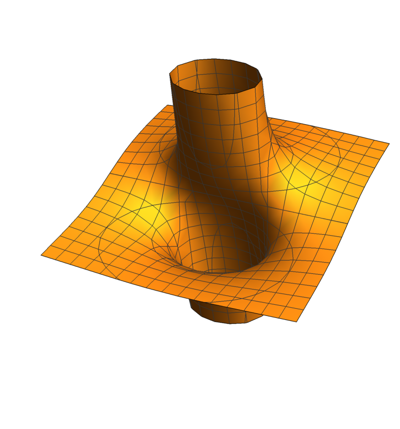
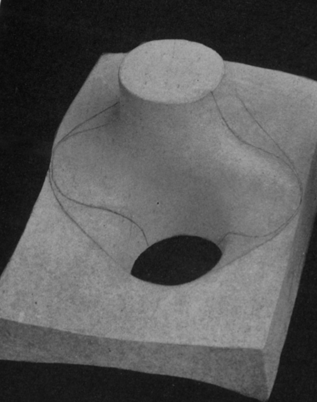
Figure 5: The cardioid surface in Example 12. On the right is Eiesland’s plaster model Eies08 .

Example 9

The following toric curve a is rational quartic with a triple point:

$$Q\,\,=\,\,x^{4}-yz^{3}.$$

Following (Little83, , Example 4.3), the abelian integrals on this curve evaluate to

$$\begin{matrix}X&=&\int sds+\int{t}dt&=&\frac{1}{2}(s^{2}+t^{2}),\vskip 3.0pt plus 1.0pt minus 1.0pt\\ Y&=&\int s^{4}ds+\int t^{4}dt&=&\frac{1}{5}(s^{5}+t^{5}),\vskip 3.0pt plus 1.0pt minus 1.0pt\\ Z&=&\int ds+\int dt&=&s+t.\end{matrix}$$

Elimination of the parameters $s$ and $t$ reveals the equation for this quintic theta surface:

$$Z^{5}-20X^{2}Z+20Y\,\,=\,\,0.$$ (29)

Little Little83 generalizes this and other theta surfaces to higher dimensions. He presents a geometric derivation of theta divisors in $\mathbb{C}^{g}$ from (degenerate) canonical curves of genus $g$.

Our next example shows how transcendental theta surfaces can degenerate to algebraic surfaces. This kind of analysis plays an important role in Eiesland’s proof of Theorem 5.1.

Example 10

We consider an irreducible rational quartic with two singular points, namely one ordinary cusp and one tacnode. The following curve has these properties for general $\lambda$:

$$q\,\,=\,\,x^{3}y+\lambda x^{4}+(1-\lambda)x^{2}y-y^{2}\qquad{\rm with}\quad q_{y}\,\,=\,\,x^{3}+(1-\lambda)x^{2}-2y.$$

Following Eiesland’s derivation in (Eies08, , Section III), we choose the rational parametrization

$$\begin{matrix}x\,\,=\,\,\frac{w^{2}\,+\,(\lambda+1)w}{w\,+\,1}\quad{\rm and}\quad y\,\,=\,\,\frac{(w^{2}\,+\,(\lambda+1)w)^{2}}{w\,+\,1}\end{matrix}$$

The differential form $dx$ can be written in terms of the curve parameter $w$ as follows:

$$\begin{matrix}dx\,\,=\,\,\bigl{(}1+\frac{\lambda}{(w+1)^{2}}\bigr{)}dw.\end{matrix}$$

We substitute these expressions into (5), and we find the three antiderivatives

$$\begin{matrix}\frac{\log(w+\lambda+1)}{\lambda+1}-\frac{\log(w)}{\lambda+1}\,,\quad-w\,,\quad\frac{(\lambda-1)\log(w+\lambda+1)}{(\lambda+1)^{3}}-\frac{(\lambda-1)\log(w)}{(\lambda+1)^{3}}-\frac{(\lambda-1)w-\lambda-1}{(\lambda+1)^{2}w^{2}+(\lambda+1)^{3}w}.\end{matrix}$$

The two generating curves are found by setting $w=s$ and $w=t$. Hence our theta surface is

$$\begin{matrix}X&=&\frac{\log(s+\lambda+1)}{\lambda+1}-\frac{\log(s)}{\lambda+1}\,\,+\,\,\frac{\log(t+\lambda+1)}{\lambda+1}-\frac{\log(t)}{\lambda+1},\vskip 3.0pt plus 1.0pt minus 1.0pt\\ Y&=&-\,s\,-t,\qquad\qquad\vskip 3.0pt plus 1.0pt minus 1.0pt\\ Z&=&\frac{(\lambda-1)\log(s+\lambda+1)}{(\lambda+1)^{3}}-\frac{(\lambda-1)\log(s)}{(\lambda+1)^{3}}-\frac{(\lambda-1)s-\lambda-1}{(\lambda+1)^{2}s^{2}+(\lambda+1)^{3}s}\vskip 3.0pt plus 1.0pt minus 1.0pt\\ &&\quad\quad+\frac{(\lambda-1)\log(t+\lambda+1)}{(\lambda+1)^{3}}-\frac{(\lambda-1)\log(t)}{(\lambda+1)^{3}}-\frac{(\lambda-1)t-\lambda-1}{(\lambda+1)^{2}t^{2}+(\lambda+1)^{3}t}.\end{matrix}$$

From this parametrization we infer that the theta surface is transcendental for $\lambda\not=-1$.

Now let $\lambda=-1$. Then $q=x^{3}y-x^{4}+2yx^{2}-y^{2}$ and the tacnode is now a node-cusp. This is a singular point obtained by merging a node and a cusp. Using the calculus identity $\,{\rm lim}_{\lambda\rightarrow-1}\bigl{\{}\frac{\log(s+\lambda+1)}{\lambda+1}-\frac{\log(s)}{\lambda+1}\bigr{\}}=\frac{d}{ds}{\rm log}(s)=\frac{1}{s}$, the parametrization of our surface becomes

$$\begin{matrix}X\,=\,\frac{1}{s}+\frac{1}{t},\quad\quad Y\,=\,-s-t,\quad\quad Z\,=\,\frac{3s+2}{6s^{3}}+\frac{3t+2}{6t^{3}}.\end{matrix}$$

Eliminating $s$ and $t$, we obtain the implicit equation.

$$2X^{3}Y+3X^{2}Y+6X^{2}-6YZ+6X\,\,=\,\,0.$$

Hence, the theta surface is a rational quartic for $\lambda=-1$, and it is transcendental for $\lambda\not=-1$.

The maximum degree of any algebraic theta surface is six. The next example attains this.

Example 11

Following Eiesland (Eies08, , p. 381–383 and VI on p. 386), we consider the quartic

$$q\,\,=\,\,(y-x^{2})^{2}\,+\,2xy(y-x^{2})\,+\,y^{3}.$$

The unique singular point, at the origin, is a tacnode cusp. The theta surface is given by

$$\begin{matrix}X&=&\int\!\frac{s+1}{s^{4}}ds\,+\,\int\!\frac{t+1}{t^{4}}dt&=&-\frac{1}{2s^{2}}-\frac{1}{3s^{3}}\,-\,\frac{1}{2t^{2}}-\frac{1}{3t^{3}},\vskip 3.0pt plus 1.0pt minus 1.0pt\\ Y&=&\int\!\frac{1}{s^{2}}ds\,+\,\int\!\frac{1}{t^{2}}dt,&=&-\frac{1}{s}\,-\,\frac{1}{t},\vskip 3.0pt plus 1.0pt minus 1.0pt\\ Z&=&\int\!\frac{2s+1}{s^{6}}ds\,+\,\int\!\frac{2t+1}{t^{6}}&=&-\frac{1}{5s^{5}}-\frac{1}{2s^{4}}\,-\,\frac{1}{5t^{5}}-\frac{1}{2t^{4}}.\\ \end{matrix}$$

The implicit equation is found to be

$$4Y^{6}-24Y^{5}-60XY^{3}+45Y^{4}+180XY^{2}-180X^{2}+180YZ-180Z\,\,\,=\,\,\,0.$$

This sextic looks different from that in (Eies08, , VI on p. 386) because of a coordinate change.

We conclude our panorama of algebraic theta surfaces with two classical cubic surfaces.

Example 12 (Cardioid Surface)

We first consider the cardioid $q=(x^{2}+y^{2}-2x)^{2}-4(x^{2}+y^{2})$. Note that $q_{y}=4x^{2}y+4y^{3}-8xy-8y$. We choose a rational parametrization as follows:

$$\begin{matrix}x\,\,=\,\,\frac{4(1-w^{2})}{(w^{2}+1)^{2}}\,,\quad\hbox{hence}\quad dx=\frac{8w(w^{2}-3)}{(w^{2}+1)^{3}}dw\,,\quad\hbox{and}\quad y\,\,=\,\,\frac{8w}{(w^{2}+1)^{2}}.\end{matrix}$$

We substitute this into the differential forms in (5), and we compute the three antiderivatives:

$$\begin{matrix}\int\frac{w^{2}-1}{2(1+w^{2})^{2}}dw=-\frac{w}{2(w^{2}+1)}\,,\quad\int\frac{-w}{(1+w^{2})^{2}}dw=\frac{1}{2(w^{2}+1)}\,,\quad\int\frac{-1}{8}dw=-\frac{w}{8}.\end{matrix}$$

Similar to the computations in the previous examples, we obtain the theta surface as follows:

$$\begin{matrix}X\,=\,-\frac{s}{2(s^{2}+1)}-\frac{t}{2(t^{2}+1)},\quad\quad Y\,=\,\frac{1}{2(s^{2}+1)}+\frac{1}{2(t^{2}+1)},\quad\quad Z\,=\,-\frac{s}{8}-\frac{t}{8},\vskip 6.0pt plus 2.0pt minus 2.0pt\\ 8X^{2}Z+8Y^{2}Z-4YZ-X\,\,=\,\,0.\end{matrix}$$

Two pictures of the cardioid surface, from the 19th and 21st century, are shown in Figure 5.

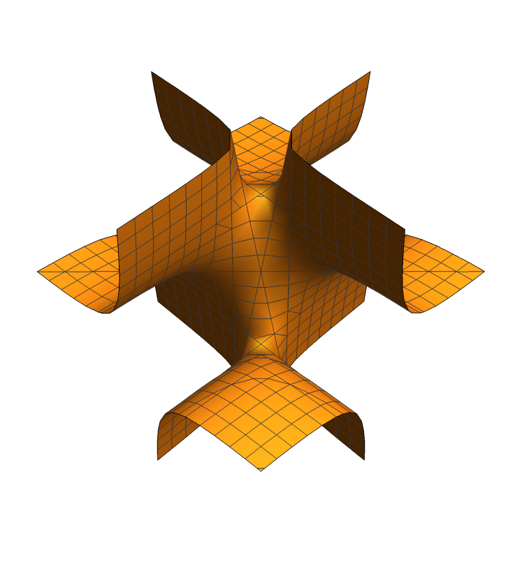
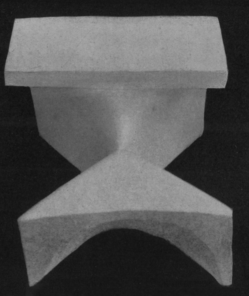
Figure 6: The Deltoid Surface. On the right ist Eiesland’s plaster model Eies08 .

Example 13 (Deltoid Surface)

We consider the deltoid curve with parametrization

$$\begin{matrix}x\,\,=\,\,\frac{4}{(w+1)^{2}},\quad{\rm and}\quad y\,\,=\,\,\frac{4}{w^{2}+6w+9}.\end{matrix}$$

This defines the quartic $\,q=y^{2}+x^{2}-2xy+x^{2}y^{2}-2x^{2}y-2xy^{2}$. The abelian integrals give

$$\begin{matrix}&X&=&\int\frac{1}{(s+1)^{2}}ds+\int\frac{1}{(t+1)^{2}}dt&=&-\frac{1}{(s+1)}-\frac{1}{(t+1)},\vskip 3.0pt plus 1.0pt minus 1.0pt\\ &Y&=&\int\frac{1}{(3+s)^{2}}ds+\int\frac{1}{(3+t)^{2}}dt&=&-\frac{1}{s+3}-\frac{1}{(t+3)},\vskip 3.0pt plus 1.0pt minus 1.0pt\\ &Z&=&\int\frac{1}{4}ds+\int\frac{1}{4}dt&=&\frac{s}{4}+\frac{t}{4}.\end{matrix}$$

Elimination yields the following cubic equation. This surface is exhibited in Figure 6:

$$4XYZ+4XY+2XZ-2YZ+3X-Y\,\,=\,\,0.$$

This equation can be transformed into the cubic $\,XYZ=a_{1}X+a_{2}Y+a_{3}Z\,$ given by Chern (Chern, , p. 2) via a linear change of coordinates, similar to that in (Eies08, , page 376, equation (11)). We saw the algebraic theta surfaces of lowest degree three in Figures 5 and 6, in views that take us back to the 19th century. We will learn more about the plaster models in Section 7.

In Section 4 we derived special transcendental theta surfaces by degenerations from Riemann’s theta function. An example was the formula for Scherk’s surface in (26). This raises the question whether our algebraic theta surfaces can be obtained in a similar manner. While the answer is affirmative, the details are complicated and we can only offer a glimpse. The role of the theta function is now played by a variant called the sigma function (naka, , §5).

We illustrate this for the singular quartic of Example 9, given by the affine equation

$$x^{4}-z^{3}\,\,=\,\,0.\qquad\qquad$$ (30)

This belongs to the family of $(3,4)$-curves (BEL, , eqn (5.1)). These plane curves are defined by

$$\qquad x^{4}-z^{3}\,+\,\lambda_{1}x^{2}z+\lambda_{2}x^{2}+\lambda_{3}xz+\lambda_{4}x+\lambda_{5}z+\lambda_{6}\,\,=\,\,0.$$ (31)

The binomial (30) is the most degenerate instance where all six coefficients $\lambda_{i}$ are zero. Such curves, and the more general $(n,s)$ curves, were introduced in the theory of integrable systems by Buchstaber, Enolski and Leykin BEL and studied further by Nakayashiki naka . They considered the sigma function associated to (31). This is an abelian function which generalizes Klein’s classical sigma function for hyperelliptic curves. The sigma function for a $(3,4)$-curve is a multigraded power series in $X,Y,Z$ whose coefficients are polynomials in $\lambda_{1},\lambda_{2},\ldots,\lambda_{6}$. By (BEL, , Example 4.5), the term of lowest degree in the sigma function equals

$$\sigma_{3,4}\,\,\,=\,\,\,\,Z^{5}\,-\,5X^{2}Z\,+\,4Y.$$

This is precisely the quintic in (29), after the coordinate scaling $(X,Y,Z)\mapsto(2X,5Y,Z)$. Thus, our algebraic theta surface arises from the sigma function by setting $\lambda_{1}=\cdots=\lambda_{6}=0$.

Similarly, the theta surface in Example 11 is closely related to the sextic $\sigma_{2,7}$ in (BEL, , Example 4.5). The polynomials $\sigma_{n,s}$ are known as Schur-Weierstrass polynomials. These play a fundamental role for rational analogs of abelian functions, and hence in the design of special solutions to the KP equation. For details we refer to BEL ; naka and the references therein. Even the genus $3$ case offers opportunities for further research. It would be interesting to revisit this topic from the perspectives of theta surfaces and tropical geometry, as in Section 4.

6 A Numerical Approach for Smooth Quartics

In this section we assume that the given quartic curve $\mathcal{Q}$ is nonsingular in $\mathbb{P}^{2}$. Then $\mathcal{Q}$ is a compact Riemann surface of genus $3$. Riemann’s Theorem 2.2 shows that its theta divisor coincides with its theta surface, up to an affine transformation. We here validate that result computationally using current tools from numerical algebraic geometry. We sample points on the theta surface using Algorithm 2 below, and we then check that Riemann’s theta function vanishes at these points using the Julia package Theta.jl by Agostini and Chua Julia .

Input: The inhomogeneous equation $q(x,y)$ of a smooth plane quartic

Output: A point on the corresponding theta surface in $\mathbb{R}^{3}$ or $\mathbb{C}^{3}$

Step 1: Specify two points $p_{1}$ and $p_{2}$ on the quartic.

Step 2: Take two other points $p_{1}^{\prime}$ and $p_{2}^{\prime}$ nearby $p_{1}$ and $p_{2}$ respectively.

Step 3: Compute the following triples of integrals numerically:

$$\begin{matrix}c_{1}&=&(\int_{p_{1}}^{p_{1}^{\prime}}\omega_{1},\int_{p_{1}}^{p_{1}^{\prime}}\omega_{2},\int_{p_{1}}^{p_{1}^{\prime}}\omega_{3}),&c_{2}&=&(\int_{p_{2}}^{p_{2}^{\prime}}\omega_{1},\int_{p_{2}}^{p_{2}^{\prime}}\omega_{2},\int_{p_{2}}^{p_{2}^{\prime}}\omega_{3}).\end{matrix}$$

Step 4: Output the sum $c_{1}+c_{2}$.

Algorithm 2 Sampling from a theta surface given its plane quartic

This algorithm is similar to Algorithm 1. However, the difference is that computation is now done by numerical evaluation. Indeed, when the polynomial $q(x,y)$ defines a smooth quartic, it is impractical to work with an algebraic formula for $y$ in terms of $x$, so we employ numerical methods even for Steps 1 and 2 above. Of course, when such an expression is available, it can be used to strengthen the numerical computations, as we will see later.

The central point of Algorithm 2 is computing the abelian integrals in Step 3. Such integrals appear throughout mathematics, from algebraic geometry to number theory and integrable systems, and there is extensive work in evaluating them numerically. Notable implementations are the library abelfunctions in SageMath SwiDec , the package algcurves in Maple DecHoe , and the MATLAB code presented in MATLAB . The software we used for our experiments is the package RiemannSurfaces in SageMath due to Bruin, Sijsling and Zotine BruSijZot .

The underlying algorithm views a plane algebraic curve $\mathcal{Q}$ as a ramified cover $\mathcal{Q}\to\mathbb{P}^{1}$ of the Riemann sphere $\mathbb{P}^{1}$ via the projection $(x,y)\mapsto x$. The package lifts paths from $\mathbb{P}^{1}$ to paths on the Riemann surface $\mathcal{Q}$ and integrates the abelian differentials in (5) along these paths via certified homotopy continuation. In order to carry this out, it is essential to avoid the ramification points of the projection to $\mathbb{P}^{1}$. This is done by computing the Voronoi decomposition of the Riemann sphere $\mathbb{P}^{1}$ given by the branch points of $\mathcal{Q}\to\mathbb{P}^{1}$. The integration paths are obtained from edges of the Voronoi cells. Avoidance of the ramification points is also a feature in the other packages such as algcurves and abelfunctions.

It is important to note that avoiding the ramification points conflicts with our desire to create real theta surfaces and to work with Riemann matrices and theta equations over $\mathbb{R}$. The cycle basis that is desirable for revealing the real structure, as in Sil , forces us to compute integrals near ramification points. We had to tweak the method in BruSijZot to make this work.

In what follows we present a case study that illustrates Algorithm 2. Our instance is the Trott curve. This is a smooth plane quartic $\mathcal{Q}$, defined by the inhomogeneous polynomial

$$q(x,y)\,\,=\,\,144(x^{4}+y^{4})-225(x^{2}+y^{2})+350x^{2}y^{2}+81.$$ (32)

The Trott curve is a widely known example of a real quartic whose $28$ bitangent lines are all real and touch at real points. It is also a M-curve, meaning that the real locus $\mathcal{Q}_{\mathbb{R}}$ has four connected components, which is the highest possible number for a real genus 3 curve.

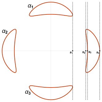
Figure 7: The Trott curve, together with some branching points and some homology cycles.

Given any M-curve $\mathcal{Q}$, there exists a symplectic basis for the homology group $H^{1}(\mathcal{Q},\mathbb{Z})$ whose associated period matrix $\Pi$ in (14) respects the real structure (cf. Sil ). With such a choice of basis, the Riemann matrix $B$ in (15) is real, and the theta function defines a surface in real $3$-space $\mathbb{R}^{3}$. According to Theorem 2.2, this surface is precisely our theta surface.

We now verify this numerically. The first step consists in identifying a real period matrix for $\mathcal{Q}$. To do so, we follow Silhol Sil . First we observe that the Trott curve is highly symmetric: its automorphism group is the dihedral group $D_{4}$, generated by the automorphisms

$$(x,y)\mapsto(x,-y),\qquad(x,y)\mapsto(-x,y),\qquad(x,y)\mapsto(-x,-y),\qquad(x,y)\mapsto(y,x).$$ (33)

We choose a symplectic basis of $H^{1}(\mathcal{Q},\mathbb{Z})$ as follows: the cycles $\alpha_{1},\alpha_{2},\alpha_{3}$ are as indicated in Figure 7, where we take $\alpha_{1},\alpha_{3}$ with clockwise orientation and $\alpha_{2}$ with counterclockwise orientation. Furthermore, referring again to Figure 7, we take $\beta_{1},\beta_{3}$ to be the two cycles lying over the interval $[s_{1},s_{2}]$ and intersecting $\alpha_{1},\alpha_{3}$ respectively. Instead, the path $\beta_{2}$ is the one lying over the interval $(-\infty,-s_{4}]\cup[s_{4},+\infty)$. Then, with these choices, there exist real numbers $a_{j}$ and purely imaginary numbers $b_{i}$ such that the two $3\times 3$ blocks in (14) satisfy

$$\Pi_{\alpha}\,=\,\begin{pmatrix}0&-a_{1}&0\,\\ -a_{1}&0&a_{1}\,\\ \,a_{2}&-a_{2}&a_{2}\,\end{pmatrix},\qquad\Pi_{\beta}\,=\,\begin{pmatrix}\,b_{1}&2b_{1}&\,b_{1}\\ b_{1}&0&-b_{1}\\ \,b_{2}&0&b_{2}\end{pmatrix}.$$ (34)

The scalars $a_{j}$ are real because the paths $\alpha_{1},\alpha_{2},\alpha_{3}$ and the differentials $\omega_{1},\omega_{2},\omega_{3}$ are real. The scalars $b_{i}$ are purely imaginary because, by construction, the paths $\beta_{1},\beta_{2},\beta_{3}$ are anti-invariant with respect to complex conjugation on $\mathcal{Q}$. The symmetries in the matrices $\Pi_{\alpha}$ and $\Pi_{\beta}$ reflect the action of the automorphism group of (33). Since $\Pi_{\alpha}$ is real and $\Pi_{\beta}$ is purely imaginary, we conclude that the Riemann matrix $\,B=-i\cdot\Pi_{\alpha}^{-1}\cdot\Pi_{\beta}\,$ has all its entries real.

At this point it should be straightforward to compute all the above explicitly. However, as we see from Figure 7, the paths that we have chosen pass through the ramification points of the projection $\mathcal{Q}\to\mathbb{P}^{1}$ to the $x$-axis. Hence, we cannot use the existing routines, such as RiemannSurfaces or abelfunctions straight away. To solve this problem we mix the numerical strategy together with the symbolic one in Algorithm 1. Indeed, since the Trott curve is highly symmetric, we can compute its points symbolically in terms of radicals: more precisely, for any $x\in\mathbb{C}$, the four corresponding points $(x,y)$ on the Trott curve are given by

$$y\,\,=\,\,\pm{\frac{\sqrt{225-350x^{2}\pm\sqrt{39556x^{4}-27900x^{2}+3969}}}{12\sqrt{2}}}.$$ (35)

With this formula, we represent the abelian integrals on the Trott curve as symbolic integrals in the single variable $x$, and we then compute these numerically. We have implemented this strategy in Maple and we found the parameters in the period matrices of (34) to be

$$a_{1} \,=\,-0.02498252478, a_{2} \,=\,0.03154914935,$$

$$b_{1} \,=\,\phantom{-}0.01384015941i, b_{2} \,=\,0.02348847438i.$$

Consequently, the Riemann matrix for the Trott with our choice of homology basis equals

$$B\,\,=\,\,\begin{pmatrix}0.926246&0.553994&0.372252\\ 0.553994&1.10799&0.553994\\ 0.372252&0.553994&0.926246\end{pmatrix}.$$

The next step is to compute some points in the theta surface $\mathcal{S}$. This can be done via Algorithm 2 using the methods of RiemannSurfaces, as long as we integrate away from the ramification points of the projection to the $x$ axis. Otherwise, we can employ again the symbolic representation of (35), together with numerical integration.

We proceed as follows: first, we can choose the points $p_{1},p_{2}$ in Algorithm 2 in such a way that the line passing through them is bitangent to $\mathcal{Q}$ and parallel to the $x$ axis. Then we compute the integrals in Algorithm 2 for points in small neighborhoods of $p_{1},p_{2}$. Further details on such computations can be found in Section 7, following the definition of an envelope in (36). The rows below are five points on $\mathcal{S}$ we obtained with Maple:

$$10^{-5}\cdot\begin{pmatrix}2.58293&\>-4.55191&\>-6.38839\\ 2.53203&\>-4.46200&\>-6.26220\\ 2.48111&\>-4.37204&\>-6.13596\\ 2.43015&\>-4.28204&\>-6.00964\\ 2.37916&\>-4.19200&\>-5.88327\end{pmatrix}.$$

The last step is to check that these points are zeroes of the theta function $\theta(\mathbf{x},B)$, up to an affine transformations. To do so, we employ the Julia package Theta.jl that is described in Julia . This package is the latest software for computing with theta functions. It is especially optimized for the case of small genus and, more importantly, for repeatedly evaluating a theta function $\theta(\mathbf{x},B)$ at multiple points $\mathbf{x}$ for the same fixed Riemann matrix $B$. This allows for a fast evaluation of the theta function which is very helpful for our problems.

In our situation, we now have a sample of points $\mathbf{x}_{1},\dots,\mathbf{x}_{N}$ on the theta surface. These are given numerically. We consider the transformed points $\Pi^{-1}_{\alpha}\mathbf{x}_{1},\dots,\Pi^{-1}_{\alpha}\mathbf{x}_{N}$. According to the proof of Riemann’s Theorem 2.2, there exists a vector $\kappa\in\mathbb{C}^{3}$ such that the translated theta function $\theta(\textbf{x}+\kappa,B)$ vanishes on $\Pi^{-1}_{\alpha}\mathbf{x}_{1},\dots,\Pi^{-1}_{\alpha}\mathbf{x}_{N}$. According to the full version of Riemann’s Theorem (Mum1, , Appendix to §3), which incorporates theta characteristics, the vector $\kappa$ can be assumed to have the form $\kappa=\frac{1}{2}\left(iB\varepsilon+\delta\right)$, where $\varepsilon,\delta\in\{0,1\}^{3}$. In particular, there are only $64$ possible choices for $\kappa$. We can check explicitly all of the $64$ possibilities.

In our experiments, we computed $N=10404$ points on the surface $\mathcal{S}$, and we evaluated

$$m(\varepsilon,\delta):=\max_{i=1,\dots,N}|\theta(\mathbf{x}_{i}+\kappa,B)|$$

for each of the 64 possible choices of $(\varepsilon,\delta)$. This was computed by Theta.jl on a standard laptop in approximately 9.6 minutes. We found that

$$m\left(\varepsilon_{0},\delta_{0}\right)\approx 6\cdot 10^{-12},\qquad\text{ for }\qquad\varepsilon_{0}=\begin{pmatrix}1\\ 1\\ 1\end{pmatrix},\,\,\delta_{0}=\begin{pmatrix}0\\ 0\\ 1\end{pmatrix}.$$

For all the other choices of the pair $\varepsilon,\delta$, we determined that $10^{-3}\leq m(\varepsilon,\delta)\leq 2$.

This computation amount to a numerical verification of Riemann’s Theorem 2.2. We have

$$\mathcal{S}=\Pi_{\alpha}\cdot(\Theta_{B}-\kappa_{0}),\qquad\text{ for }\,\,\kappa_{0}=\frac{1}{2}\left(iB\varepsilon_{0}+\delta_{0}\right).$$

To conclude, this gives also a real analytic equation for $\mathcal{S}$. Indeed, for any $\kappa=\frac{1}{2}\left(iB\varepsilon+\delta\right)$, the translated theta divisor $\Theta_{B}-\kappa$ is cut out by the theta function with characteristic

$$\theta[\varepsilon,\delta](\mathbf{x},B) =\sum_{n\in\mathbb{Z}^{3}}\mathbf{e}\left(-\frac{1}{2}\left(n+\frac{\varepsilon}{2}\right)^{t}B\left(n+\frac{\varepsilon}{2}\right)+i\left(n+\frac{\varepsilon}{2}\right)^{t}\left(\mathbf{x}+\frac{\delta}{2}\right)\right)$$

$$=\sum_{n\in\mathbb{Z}^{3}}\exp\left(-\pi\left(n+\frac{\varepsilon}{2}\right)^{t}B\left(n+\frac{\varepsilon}{2}\right)\right)\cdot\cos\left(2\pi\left(n+\frac{\varepsilon}{2}\right)^{t}\left(\mathbf{x}+\frac{\delta}{2}\right)\right).$$

This is a real analytic function since the matrix $B$ is real.

7 Sophus Lie in Leipzig

Felix Klein held the professorship for geometry at the University of Leipzig until 1886 when he moved to Göttingen. In the same year, Sophus Lie was appointed to be Klein’s successor and he moved from Christiania (Oslo) to Leipzig. Lie also became one of the three directors of the Mathematical Seminar, an institution that Felix Klein had founded with the aim of strengthening the connection between education and research. In his first years at Leipzig, Lie was busy with completing his major work Theory of Transformation Groups with the assistance of Friedrich Engel. It was released in three volumes in 1888, 1890 and 1893. Thereafter, the subject of double translation surfaces moved back in the focus of his teaching and research, and it caught the attention of the mathematical community for the first time.

In what follows we discuss notable historical developments, we revisit Lie’s pre-Leipzig work on these surfaces, and we show how it relates to our discussion in the previous sections. In 1892 Lie published an article explaining how theta surfaces can be parametrized by abelian integrals (LieGes2, , p. 481). He invited two of his Leipzig students, Richard Kummer and Georg Wiegner, to rework the classification he had given in 1882 by means of abelian integrals. The work of Kummer and Wiegner was published in their doctoral theses Kum ; Wie . Under the supervision of Lie’s assistant Georg Scheffers, the two students also constructed a series of twelve plaster models that visualize the diverse shapes exhibited by theta surfaces. It is surprising that the models were commissioned by Lie, who, unlike his predecessor Klein, had not been known for an engagement in popularizing mathematics in this manner.

The collection of mathematical models at the University of Leipzig was initiated by Felix Klein in 1880. At the end of the 19th century, the collection included around $350$ models and drawings. During the 20th century, many models were lost or broken. A project for cataloging and restoring the collection was initiated by Silvia Schöneburg in 2014. A catalogue describing all $240$ remaining models is expected to be published in 2021. There are some very rare models in the collection, among them nine of the surfaces created by Lie’s students. These plaster models and their mathematics are the topic of the third author’s diploma thesis Struwe , submitted to Leipzig University in 2020. It was her find of the models by Kummer and Wiegner that brought us together for our project on theta surfaces.

In 1895 Poincaré presented his proof of the relation between double translation surfaces and Abel’s Theorem Poin1895 ; Poin95 . This led to the idea that these surfaces can be seen as theta divisors of Jacobians (Chern, , p.2). Darboux Darb and Scheffers Sch also published variants of the proof. Eiesland Eies08 ; Eies09 completed the classification initiated by Kummer and Wiegner. He also constructed plaster models for some of his surfaces (cf. Figures 5 and 6). Eiesland’s plaster models of theta surfaces were donated to the collection at John Hopkins University.

Later on, our theme found its way into modern research. Shiing-Shen Chern Chern characterized theta surfaces in terms of the web geometry that was developed by Blaschke and Bol in the 1930’s. In 1983, John Little Little83 studied the theory for curves of genus $g\geq 3$, and he proposed a solution of the Schottky problem of recognizing Jacobians in terms of translation manifolds. More precisely, he showed that a principally polarized abelian variety of dimension $g$ is the Jacobian of a non-hyperelliptic curve if and only if its theta divisor can be written locally as a Minkowski sum of $g-1$ analytic curves. Little’s article Little92 connects this point of view to the integrable systems approach (cf. DFS ) to the Schottky problem.

The doctoral theses of Kummer and Wiegner built on Lie’s earlier results. One of these is the recovery of generating curves for a theta surface $\mathcal{S}$ from the equation of $\mathcal{S}$ by means of differential geometry. This was helpful for constructing real surfaces in situations when the abelian integrals delivered complex values. We state Lie’s result using a slight modification of the set-up in Section 2. Fix a quartic $\mathcal{Q}\subset\mathbb{P}^{2}$ and let $\mathcal{L}(0)$ be a line that is tangent to $\mathcal{Q}$ at a smooth point $p_{1}(0)$ and intersects $\mathcal{Q}$ in other two points $p_{3}(0),p_{4}(0)$. Using the points $p_{1}(z)$ near $p_{1}(0)$, where $z$ is a local coordinate, we obtain a parametrization as in (8):

$$(s,t)\,\,\mapsto\,\,\,\Omega_{1}(p_{1}(s))\,+\,\Omega_{1}(p_{1}(t)).$$ (36)

The surface $\mathcal{S}$ is the Minkowski sum $\mathcal{S}=\mathcal{C}+\mathcal{C}$, where $\mathcal{C}$ is the curve $z\mapsto\Omega_{1}(p_{1}(z))$. The scaled curve $2\cdot\mathcal{C}$ lies in $\mathcal{S}$. This curve was called an envelope by Lie.

In classical differential geometry, an asymptotic curve on a surface $\mathcal{S}$ is a curve whose tangent direction at each point has normal curvature zero on $\mathcal{S}$. This means that the tangent direction at each point is isotropic with respect to the second fundamental form of $\mathcal{S}$.

Theorem 7.1 (Lie)

Let $\mathcal{S}=\mathcal{C}+\mathcal{C}$ be the theta surface given by the parametrization (36). Then the envelope $\,2\cdot\mathcal{C}\,$ is an asymptotic curve of the surface $\mathcal{S}$.

This result appears in (LieGes2, , p. 211), albeit in a different formulation that emphasizes minimal surfaces. Our version in Theorem 7.1 was presented by Kummer in (Kum, , p. 15).

Lie’s reconstruction is remarkable in that it solves Torelli’s problem for genus $3$ curves. Indeed, Lie found his result several decades before Torelli Tor proved his famous theorem in algebraic geometry. Torelli’s problem asks to recover an algebraic curve $\mathcal{C}$ from its Jacobian $J(\mathcal{C})$ together with the theta divisor $\Theta\subset J(\mathcal{C})$. In our situation, once we recover the envelope $\mathcal{C}$ as the asymptotic curve of the surface $\mathcal{S}$, we can reconstruct the quartic curve $\mathcal{Q}$ as in Remark 3. Note that this reconstruction technique also works for singular quartics.

Algebraic geometers will notice a connection between Lie’s approach and Andreotti’s geometric proof Andr of Torelli’s theorem. Indeed, the second fundamental form of $\mathcal{S}$ is the differential of the Gauss map $\,\mathcal{S}\rightarrow{(\mathbb{P}^{2})}^{*}$. This map associates to each point of $\mathcal{S}$ its tangent space in $\mathbb{C}^{3}$. Andreotti observed that the Gauss map of the theta divisor $\Theta\subset J(\mathcal{C})$ is branched precisely over the curve in ${(\mathbb{P}^{2})}^{*}$ dual to $\mathcal{C}\subset\mathbb{P}^{2}$. Hence $\mathcal{C}$ can be recovered thanks to the biduality theorem. It would be interesting to further study Lie’s differential-geometric approach to the Torelli problem via the Gauss map. One natural question is whether Theorem 7.1 extends to curves of higher genus and how this relates to Andreotti’s method.

Example 14

To illustrate Lie’s result, we determine an envelope for Scherk’s minimal surface directly from the equation (1). After computing the second fundamental form, we see that a curve $(X(t),Y(t),Z(t))$ in the surface is asymptotic if and only if it satisfies

$$\frac{\dot{X}(t)^{2}}{\sin^{2}(X(t))}\,=\,\frac{\dot{Y}(t)^{2}}{\sin^{2}(Y(t))}\,,\quad\text{ or equivalently }\quad\frac{\dot{X}(t)}{\sin(X(t))}\,=\,\pm\frac{\dot{Y}(t)}{\sin(Y(t))}.$$

The solutions to this differential equation are given by the following two families of curves:

$$\frac{\tan\left(X/2\right)}{\tan\left(Y/2\right)}\,=\,c\qquad{\rm and}\qquad\tan\left(\frac{X}{2}\right)\cdot\tan\left(\frac{Y}{2}\right)\,=\,c\qquad{\rm for}\quad c\in\mathbb{R}\setminus\{0\}.$$

Consider a curve from the first family. Setting $X=2\arctan(t)$, we can parametrize it as

$$\left(2\arctan(t)\,,\,\,2\arctan\left(\frac{t}{c}\right)\,,\,\,\log\left(\frac{c^{2}+t^{2}}{c(t^{2}+1)}\right)\right).$$

The last expression comes from the fact that $Z=\log\left(\frac{\sin(X)}{\sin(Y)}\right)$ holds on Scherk’s surface. Now, setting $c=\frac{1}{5}$ and using Theorem 7.1, we obtain the generating curve $\mathcal{C}$ given by

$$\left(\arctan(t),\arctan\left(5t\right),\frac{1}{2}\log\left(\frac{1+(5t)^{2}}{5(t^{2}+1)}\right)\right).$$

The resulting representation $\mathcal{S}=\mathcal{C}+\mathcal{C}$ is precisely the one we presented in equation (4).

Already in 1869, Lie studied the parametrization of tetrahedral theta surfaces

$$\mathcal{S}\,\,=\,\,\bigl{\{}\,\alpha\cdot\exp(X)\,+\,\beta\cdot\exp(Y)\,+\,\gamma\cdot\exp(Z)\,=\,\delta\,\bigr{\}}.$$ (37)

Here $\alpha,\beta,\gamma,\delta$ are nonzero constants. These surfaces play a prominent role in Theorem 4.1. The adjective “tetrahedral” refers to the fact that the Delaunay polytope is a tetrahedron. Example 5 shows that Scherk’s surface is tetrahedral, after a coordinate change over $\mathbb{C}$.

Lie proved that tetrahedral theta surfaces admit infinitely many representations $\mathcal{S}=\mathcal{C}_{1}+\mathcal{C}_{2}$. This was already mentioned in Remark 4. We present Lie’s method for identifying these infinitely many pairs of generating curves. A key tool is the logarithmic transformation

$$X=\log(U),\quad Y=\log(V),\quad Z=\log(W).$$

This transforms the surface $\mathcal{S}\subset\mathbb{C}^{3}$ into the plane $\mathcal{P}\subset(\mathbb{C}^{*})^{3}$ defined by the equation

$$\mathcal{P}\,\,=\,\,\bigl{\{}\,\alpha\cdot U\,+\,\beta\cdot V\,\,+\,\,\gamma\cdot W\,=\,\delta\,\bigr{\}}.$$ (38)

The generating curves in $\mathcal{S}=\mathcal{C}_{1}+\mathcal{C}_{2}$ correspond to curves $\mathcal{D}_{1},\mathcal{D}_{2}$ such that $\mathcal{P}=\mathcal{D}_{1}\cdot\mathcal{D}_{2}$. Here $\mathcal{D}_{1}\cdot\mathcal{D}_{2}$ denotes the Hadamard product of the two curves, i.e. the set obtained from the coordinatewise product of all points in $\mathcal{D}_{1}$ with all points in $\mathcal{D}_{2}$. Lie studied this alternative formulation and found infinitely many pair of lines $\mathcal{D}_{1},\mathcal{D}_{2}\subset(\mathbb{C}^{*})^{3}$ such that $\mathcal{P}=\mathcal{D}_{1}\cdot\mathcal{D}_{2}$.

We shall state Lie’s result more precisely. The action of the group of translations on $\mathbb{C}^{3}$ corresponds under the logarithmic transformation to the action of the torus $(\mathbb{C}^{*})^{3}$ on itself. Thus, we are free to rescale the coordinates $U,V,W$. In particular, we can assume that our plane $\mathcal{P}$ and the desired lines $\mathcal{D}_{1}$ and $\mathcal{D}_{2}$ contain the point $\mathbf{1}=(1,1,1)$. With this, the identity $\mathcal{P}=\mathcal{D}_{1}\cdot\mathcal{D}_{2}$ implies $\mathcal{D}_{1},\mathcal{D}_{2}\subset\mathcal{P}$. On the theta surface side, this corresponds to translating the surface and the curves until all of them pass through the origin $\mathbf{0}=(0,0,0)$.

We next consider the closure of the plane $\mathcal{P}$ and the lines $\mathcal{D}_{1},\mathcal{D}_{2}$ inside the projective space $\mathbb{P}^{3}$ with coordinates $U,V,W,T$. The arrangement of coordinate planes $\{UVWT=0\}$ in $\mathbb{P}^{3}$ intersects our plane $\mathcal{P}$ in four lines $\mathcal{H}_{1},\mathcal{H}_{2},\mathcal{H}_{3},\mathcal{H}_{4}$. Here now is the promised result.

Theorem 7.2 (Lie)

Let $\mathcal{D}_{1},\mathcal{D}_{2}$ be lines through $\mathbf{1}=(1:1:1:1)$ in $\mathcal{P}$. Then $\mathcal{P}=\mathcal{D}_{1}\cdot\mathcal{D}_{2}$ if and only if the six lines $\,\mathcal{D}_{1},\mathcal{D}_{2},\,\mathcal{H}_{1},\mathcal{H}_{2},\mathcal{H}_{3},\mathcal{H}_{4}\,$ are tangent to a common conic in $\,\mathcal{P}$.

This result is featured in (LieGes2, , p. 526). We here present a self-contained proof.

Proof

We identify $\mathcal{P}$ with the affine plane with coordinates $s$ and $t$ by setting

$$U\,=\,1+as+bt\,,\,\,\,V\,=\,1+cs+dt\,,\,\,\,W\,\,=\,\,1+es+ft\quad{\rm and}\quad T=1.$$ (39)

The origin $(s,t)=(0,0)$ corresponds to the distinguished point ${\bf 1}$. The two lines of interest are $\mathcal{D}_{1}=\{s=0\}$ and $\mathcal{D}_{2}=\{t=0\}$. The four coordinate lines are $\mathcal{H}_{1}=\{U=0\}$, $\mathcal{H}_{2}=\{V=0\}$, $\mathcal{H}_{3}=\{W=0\}$, and $\mathcal{H}_{4}$ is the line at infinity in the $(s,t)$-plane. Thus, the six scalars $a,b,c,d,e,f$ in (39) specify the inclusions $\,\mathcal{D}_{1},\mathcal{D}_{2}\subset\mathcal{P}\subset\mathbb{P}^{3}$. With these conventions, $\,\mathcal{D}_{1},\mathcal{D}_{2},\,\mathcal{H}_{1},\mathcal{H}_{2},\mathcal{H}_{3},\mathcal{H}_{4}\,$ are tangent to a common conic in $\mathcal{P}$ if and only if

$${\rm det}\begin{pmatrix}a&b&ab\\ c&d&cd\\ e&f&ef\end{pmatrix}\,\,=\,\,0.$$ (40)

The Hadamard product $\,\mathcal{D}_{1}\cdot\mathcal{D}_{2}\,$ is a surface in $\mathbb{P}^{3}$. It has the parametric representation

$$\tilde{U}\,=\,(1+as)(1+bt)\,,\,\,\,\tilde{V}\,=\,(1+cs)(1+dt)\,,\,\,\,\tilde{W}\,=\,(1+es)(1+ft)\,,\,\,\,\tilde{T}=1.$$ (41)

This can be rewritten as

$$\tilde{U}\,=\,U\,+\,ab\cdot st\,,\,\quad\tilde{V}\,=\,V\,+\,cd\cdot st\,,\,\quad\tilde{W}\,=\,W\,+\,ef\cdot st\,,\,\quad\tilde{T}\,=\,T.$$

Hence the surface $\,\mathcal{D}_{1}\cdot\mathcal{D}_{2}\,$ equals the plane $\mathcal{P}$ in $\mathbb{P}^{3}$ if and only if the point $(ab:cd:ef:0)$ lies in $\mathcal{P}$. This happens if and only if the condition (40) holds. Now the proof is complete.

Given the tetrahedral theta surface (37), we can now construct a one-dimensional family of pairs $\mathcal{C}_{1},\mathcal{C}_{2}$ of generating curves. The corresponding line pairs $\mathcal{D}_{1},\mathcal{D}_{2}$ in the plane (38) are found as follows. We consider the one-dimensional family of conics that are tangent to $\mathcal{H}_{1},\mathcal{H}_{2},\mathcal{H}_{3},\mathcal{H}_{4}$. Each such conic has tangent lines pass through $\mathbf{1}$. These are $\mathcal{D}_{1}$ and $\mathcal{D}_{2}$.

In the algebraic formulation above, the geometric constraints can be solved as follows. The given theta surface (37) is specified by any solution to $\alpha+\beta+\gamma=\delta$. The desired one-dimensional family is the solution set to five equations in the six unknowns $a,b,c,d,e,f$. In order for the planes in (39) and (38) to agree, we need $\,\alpha a+\beta c+\gamma e\,=\,\alpha b+\beta d+\gamma f\,=\,0$. To get unique parameters for our lines, we may also fix $a$ and $f$ in $\mathbb{C}$. Finally, the quadratic equation (40) must be satisfied. These five constraints define a curve in $\mathbb{C}^{6}$ whose points are the solutions $\,(\mathcal{D}_{1},\mathcal{D}_{2})\,$ to $\,\mathcal{D}_{1}\cdot\mathcal{D}_{2}=\mathcal{P}\,$ and hence the solutions $\,(\mathcal{C}_{1},\mathcal{C}_{2})\,$ to $\,\mathcal{C}_{1}+\mathcal{C}_{2}=\mathcal{S}$.

We demonstrate this algorithm for computing generating curves of (37) in an example.

Example 15

We revisit Example 2 and the corresponding tetrahedral theta surface given (20). After replacing $Z$ with $Z+\log(3)$, the resulting surface passes through $\mathbf{0}$. We have

$$\begin{matrix}\mathcal{S}&=&\,\,\{\,\exp(X)\,+\,\exp(Y)\,-\,3\exp(Z)\,+\,1\,\,=\,\,0\,\}&\subset\,\,\mathbb{C}^{3},\vskip 3.0pt plus 1.0pt minus 1.0pt\\ \mathcal{P}&=&\{\,U\,+\,V\,-\,3W\,+\,T\,\,=\,\,0\,\}&\subset\,\,\mathbb{P}^{3}.\end{matrix}$$

To find a valid parametrization of $\mathcal{P}$ as in (41), we consider the equations in $a,b,c,d$, $e,f$ described above. We fix $a=1,f=0$ and we leave $b$ unspecified. The remaining parameters are determined as $\,c=1$, $\,d=-b$, $\,e=2/3$, by requiring (40) and that (41) lies on $\mathcal{P}$.

We conclude that the plane $\mathcal{P}$ has the parametrizations

$$\tilde{U}\,=\,(1+s)\cdot(1+bt)\,,\,\tilde{V}\,=\,(1+s)\cdot(1-bt)\,,\,\tilde{W}\,=\,\left(1+\frac{2}{3}s\right)\cdot 1,\,\hbox{for all}\,\,\,\quad b\in\mathbb{C}\backslash\{0\}.$$

Our tetrahedral theta surface $\mathcal{S}$ has the one-dimensional family of parametrizations:

$$X\,=\,{\rm log}(1+s)\,+\,{\rm log}(1+bt)\,,\quad Y\,=\,{\rm log}(1+s)\,+\,{\rm log}(1-bt)\,,\quad Z\,=\,{\rm log}\left(1+\frac{2}{3}s\right).$$

This example is admittedly quite special, but the method works for all tetrahedral theta surfaces, i.e. whenever the quartic curve $\mathcal{Q}$ is among the last three types in Figures 2 and 3.

We conclude this article by returning to the twelve plaster models of theta surfaces constructed by the doctoral students of Sophus Lie at Leipzig in 1892. In Figure 8 we display one model due to Richard Kummer Kum and one model due to Georg Wiegner Wie .

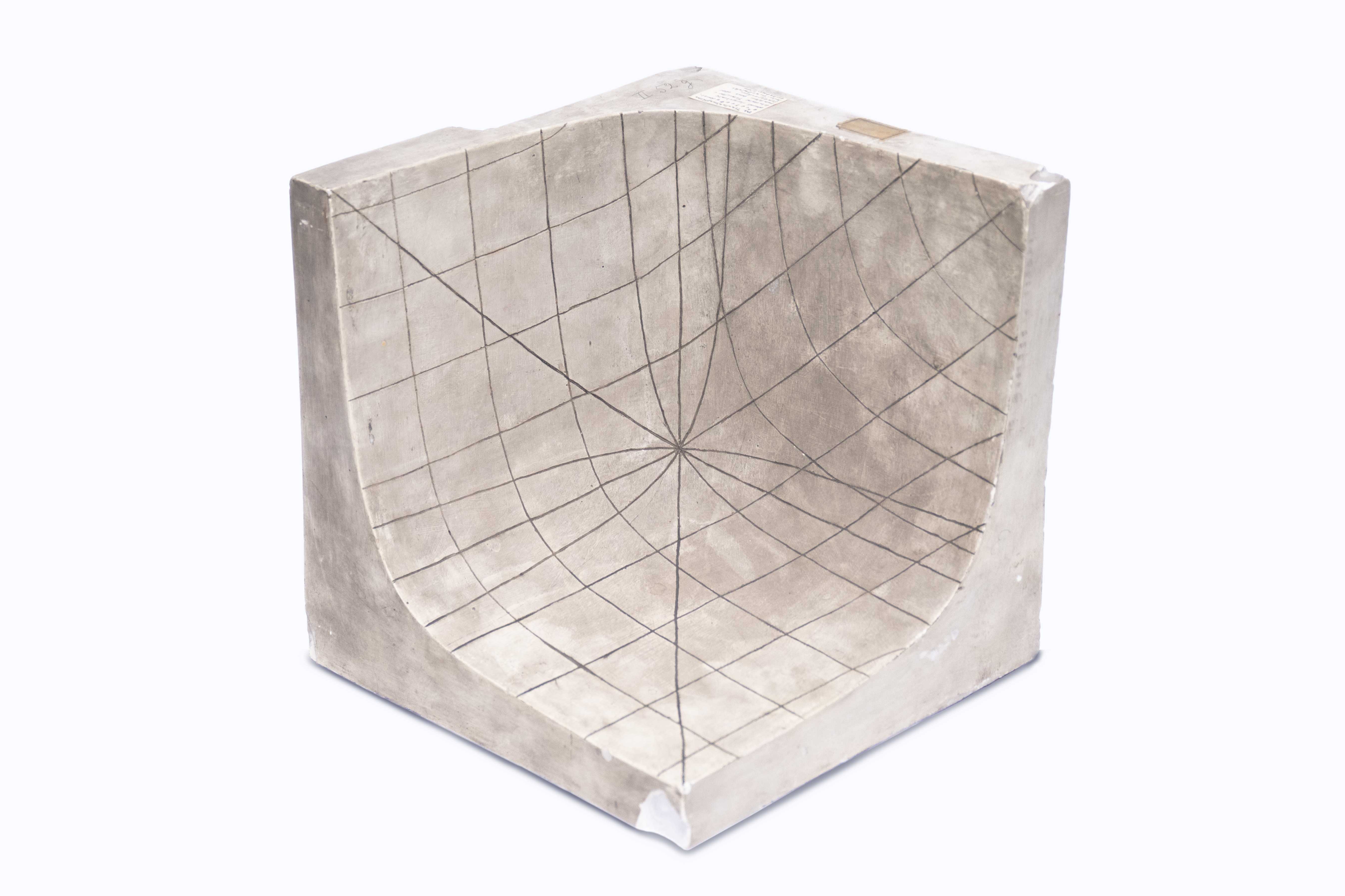
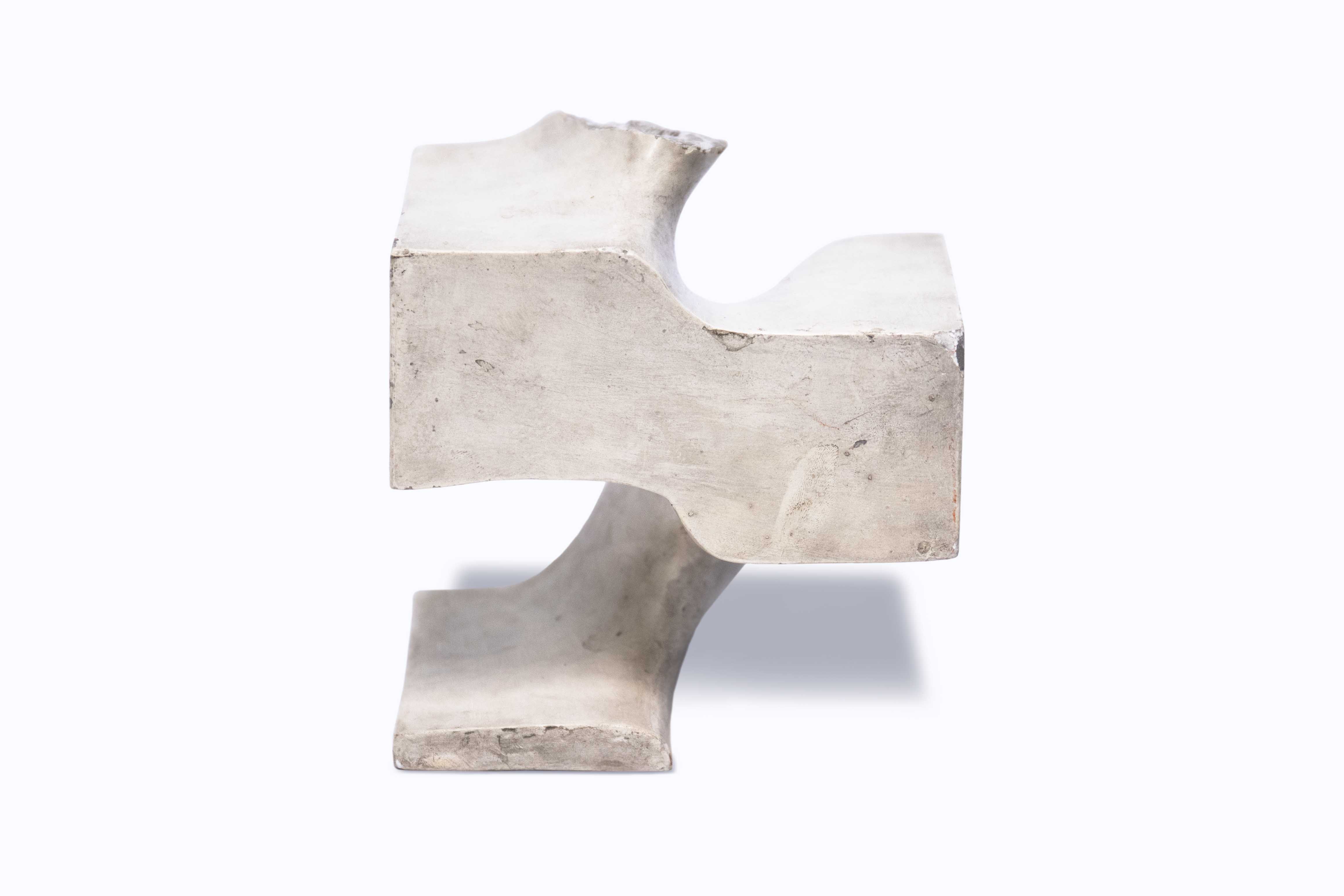
Figure 8: Plaster models of theta surfaces constructed in the 1890s by Lie’s students Kummer (left) and Wiegner (right). These models are still in the collection at Universität Leipzig.

The model on the left in Figure 8 shows the tetrahedral theta surface

$$\mathcal{S}\quad=\quad\bigl{\{}\,10^{-X}+10^{-Y}+10^{-Z}\,=\,1\,\bigr{\}}.$$

Kummer derives this surface in (Kum, , Section III.6) from a pencil of conics like in Example 2. In (Kum, , p. 32) he applies a particular transformation to the surface, which seems to be advantageous for the practical construction of a plaster model. The one-dimensional family of Minkowski decompositions $\,\mathcal{S}=\mathcal{C}_{1}+\mathcal{C}_{2}\,$ into curves can be found using our algorithm for Theorem 7.2. The model on the right in Figure 8 shows another theta surface, namely

$$\mathcal{S}\quad=\quad\biggl{\{}\,{\rm tan}(Z)\,+\,\frac{2X}{X^{2}+2Y}\,\,=\,\,0\,\biggr{\}}.$$

Wiegner derives this equation in (Wie, , Section IV.11) from a quartic $\mathcal{Q}$ that decomposes into a cubic curve and one of its flex lines. In (Wie, , Section II.4), Wiegner rederives the Weierstrass normal form, and he fixes the flex line to be the line at infinity. For the surface $\mathcal{S}$ he starts with the rational cubic $\,q=y^{2}-x^{2}(x-1)$, and he ends up on (Wie, , p. 65) with the equation seen above. The surface $\mathcal{S}$ is shown in (Wie, , Figure II, Tafel A). In his appendix (Wie, , p. 82), Wiegner offers a delightful description of how one actually builds a plaster model in practice.

This final section connects the 19th century with the 21st century, and differential geometry with algebraic geometry. Theta surfaces are beautiful objects, not just for 3D printing, but they offer new vistas on the moduli space of genus $3$ curves. The explicit degenerations in Sections 4 and 5, and the tools from numerical algebraic geometry in Section 6, should be useful for many applications, such as three-phase solutions of the KP equation DFS .

Acknowledgments: We are thankful to the referees for their helpful comments and remarks. We are grateful to John Little for informing us of the quadric double translation surfaces of Example 8 and to Evgeny Ferapontov for mentioning his paper BalFer to us.

References

- (1)
- (2) D. Agostini and L. Chua: Computing theta functions with Julia, arXiv:1906.06507, (2019).
- (3) A. Andreotti: On a theorem of Torelli, Am. J. Math. 80, 801–828 (1958).
- (4) E. Arbarello, M. Cornalba and P.A. Griffiths: Geometry of Algebraic Curves, Volume II, Springer, (2011).
- (5) A. Balk and E. Ferapontov: Invariants of 4-wave interactions, Physica D, 65, 274–288 (1993).
- (6) B. Bolognese, M. Brandt and L. Chua: From curves to tropical Jacobians and back, in Combinatorial Algebraic Geometry, Fields Inst. Commun. Springer New York, 21–45 (2017).
- (7) N. Bruin, J. Sijsling and A. Zotine: Numerical computation of endomorphism rings of Jacobians, Proceedings of the 13th Algorithmic Number Theory Symposium (ANTS), Open Book Ser. 2, 155–171 (2019).
- (8) V.M. Buchstaber, V.Z. Enolski and D.V. Leykin: Rational analogs of abelian functions, Funct. Anal. its Appl. 33, 83–94 (1999).
- (9) M. Chan: Combinatorics of the tropical Torelli map, Algebra Number Theory 6, 1133–1169, (2012).
- (10) S.-S. Chern: Web geometry, Bull. Am. Math. Soc. 6, 1–8 (1982).
- (11) G. Darboux: Leçons sur la théorie générale des surfaces, 2nd edition, Gauthier-Villars, (1914).
- (12) B. Deconinck and M. van Hoeij: Computing Riemann matrices of algebraic curves, Physica D 152/153, 2–46 (2001) .
- (13) B. Dubrovin, R. Flickinger and H. Segur: Three-phase solutions of the Kadomtsev-Petviashvili equation, Stud. Appl. Math. 99, 137–203 (1997).
- (14) J. Eiesland: On a certain class of algbraic translation surfaces, Am. J. Math. 29, 363-386 (1908).
- (15) J. Eiesland: On translation surfaces connected with a unicursal quartic, Am. J. Math. 30 170–208 (1909).
- (16) J. D. Fay: Theta functions on Riemann Surfaces, Springer, (1973).
- (17) J. Frauendiener and C. Klein: Algebraic curves and Riemann surfaces in Matlab, in Computational Approach to Riemann Surfaces, Lecture Notes in Math. 2013, Springer, (2011).
- (18) S. Grushevsky and K. Hulek: Principally polarized semi-abelic varieties of small torus rank, and the Andreotti-Mayer loci, Pure Appl. Math. Q. 7, 1309–1360 (2011).
- (19) R. Kummer: Die Flächen mit unendlichvielen Erzeugungen durch Translation von Kurven, Dissertation, Universität Leipzig, (1894).
- (20) S. Lie: Gesammelte Abhandlungen, 1. Abteilung, Teubner Verlag, Leipzig, (1934).
- (21) S. Lie: Gesammelte Abhandlungen, 2. Abteilung, Teubner Verlag, Leipzig, (1937).
- (22) J. Little: Translation manifolds and the converse to Abel’s theorem, Compos. Math. 49, 147–171 (1983).
- (23) J. Little: Another relation between approaches to the Schottky problem, arXiv:9202010, (1992).
- (24) D. Mumford: Tata Lectures on Theta, I, Birkhäuser, (1983).
- (25) A. Nakayashiki: On algebraic expressions of sigma functions for curves, Asian J. Math. 14, 175–212 (2010).
- (26) H. Poincaré: Fonctions abeliennes, J. Math. Pures Appl. 5, 219–314 (1895).
- (27) H. Poincaré: Sur les surfaces de translation et les fonctions abéliennes, Bull. Soc. Math. Fr. 29, 61–86 (1901).
- (28) G. Scheffers: Das Abel’sche Theorem und das Lie’sche Theorem über Translationsflächen, Acta Math. 28 65–91 (1904).
- (29) R. Silhol: The Schottky problem for real genus 3 M-curves, Math. Z. 236, 841–881 (2001).
- (30) J. Struwe: The Double Translation Surfaces of Sophus Lie, Diploma Thesis, Universität Leipzig, (2020).
- (31) C. Swierczewski and B. Deconinck: Computing Riemann theta functions in Sage with applications, Math Comput Simul 127, 263–272 (2016).
- (32) R. Torelli: Sulle varietà di Jacobi, Rendiconti della Reale accademia nazionale dei Lincei 22, 98–103, (1913).
- (33) F. Vallentin: Sphere Coverings, Lattices, and Tilings, Dissertation, TU Munich, (2003).
- (34) G. Wiegner: Über eine besondere Klasse von Translationsflächen, Dissertation, Universität Leipzig, (1895).