Kinetic models of tangential discontinuities in the solar wind

Abstract

Kinetic-scale current sheets observed in the solar wind are frequently approximately force-free despite the fact that their plasma $\beta$ is of the order of one. In-situ measurements have recently shown that plasma density and temperature often vary across the current sheets, while the plasma pressure is approximately uniform. In many cases these density and temperature variations are asymmetric with respect to the center of the current sheet. To model these observations theoretically we develop in this paper equilibria of kinetic-scale force-free current sheets that have plasma density and temperature gradients. The models can also be useful for analysis of stability and dissipation of the current sheets in the solar wind.

1 Introduction

The early in-situ measurements in the solar wind indicated the ubiquity of magnetic field discontinuities or, equivalently, current sheets with spatial scales below a few tens of ion thermal gyroradii or ion inertial lengths (e.g., Burlaga et al., 1977; Tsurutani & Smith, 1979; Lepping, 1986). The magnetic reconnection within these kinetic-scale structures may provide ion and electron heating (e.g., Osman et al., 2011; Gosling, 2012; Pulupa et al., 2014), though the overall contribution of the current sheets to the solar wind heating is unknown (e.g., Cranmer et al., 2009). The disruption of the kinetic-scale current sheets via the magnetic reconnection is potentially a mechanism resulting in the spectral break of the magnetic field turbulence spectrum at ion scales (e.g., Mallet et al., 2017; Franci et al., 2017; Vech et al., 2018). The mechanisms responsible for formation of the current sheets include Alfven wave steepening (e.g., Medvedev et al., 1997) and the natural appearance of sheet-like structures in the course of development of the turbulence cascade (e.g., Greco et al., 2009, 2016; Franci et al., 2017).

The early in-situ measurements focused on classifying the current sheets in terms of tangential and rotational discontinuities based on the analysis of the magnetic field component perpendicular to the current sheet plane (e.g., Tsurutani & Smith, 1974; Burlaga et al., 1977; Lepping, 1986). However, the estimates of the fraction of tangential and rotational discontinuities in the solar wind are still controversial (e.g., Knetter et al., 2004; Neugebauer, 2006; Artemyev et al., 2019b). The in-situ measurements unambiguously showed that current sheets in the solar wind are often approximately one-dimensional and force-free, i.e. the current density is mostly parallel to the magnetic field and the magnetic field rotates across a current sheet, while its magnitude remains constant (e.g., Burlaga et al., 1977; Lepping, 1986; Neugebauer, 2006; Paschmann et al., 2013). Recent statistical analyses (Artemyev et al., 2018, 2019b) have shown that the plasma density $n$ and ion and electron temperatures $T_{i,e}$ typically vary across a current sheet. In these analyses it was also shown that the density and temperature variations are anti-correlated $\Delta T_{i,e}/T_{i,e}\propto-\Delta n/n$, so that the plasma pressure is essentially uniform across the current sheets as required by the pressure balance.

Within the large number of known one-dimensional kinetic current sheet models (e.g., Lemaire & Burlaga, 1976; Bobrova & Syrovatskiǐ, 1979; Roth et al., 1996; Kocharovsky et al., 2010; Panov et al., 2011), the most relevant to

the solar wind observations mentioned above are the recently developed models of force-free current sheets representing tangential (Harrison & Neukirch, 2009a; Wilson & Neukirch, 2011; Allanson et al., 2015) and rotational (Artemyev, 2011; Vasko et al., 2014) discontinuities. In these kinetic models of both force-free tangential and rotational discontinuities the plasma density and temperature are uniform across the current sheet.

We remark that there is a much broader class of collisionless tangential discontinuity models (Roth et al., 1996) that can in principle be used to describe magnetic fields of solar wind discontinuities (De Keyser et al., 1996; De Keyser & Roth, 1997) and does even allow for the inclusion of plasma velocity shear (De Keyser et al., 1997, 2013), which is observed for some solar wind discontinuities (De Keyser et al., 1998; Paschmann et al., 2013; Artemyev et al., 2019b).

These models start from specifying the dependence of the distribution functions on the constants of motion and have been developed to give a detailed description different plasma populations in magnetic current sheets (Roth et al., 1996). When starting from specifying the particle distribution functions any self-consistent model of a collisionless configuration has to be completed by solving Maxwell’s equations. With the form of the distribution functions used for a detailed description of current sheets (see e.g. the model-data comparison in De Keyser et al., 1996, 1997) it is usually not possible to obtain analytical solutions for the electromagnetic fields and hence these have to be determined using numerical methods. This in turn implies that the exact spatial variation of the particle densities, the pressure and the temperature is only available after the numerical calculation of the electromagnetic fields has been carried out.

In this paper we use a different approach, mainly for two reasons. Firstly, as already mentioned above, the magnetic field configuration of many of the current sheets observed in the solar wind is observed to be force-free to a good approximation (e.g., Artemyev et al., 2019a). For one-dimensional tangential discontinuities this directly implies that the magnetic field strength $|\mathbf{B}|$ and the plasma pressure do not vary across the discontinuity (see e.g. Harrison & Neukirch, 2009b; Neukirch et al., 2018). This puts additional constraints on the possible dependence of the particle distribution functions on the constants of motion and makes finding such distribution functions for force-free magnetic field configurations non-trivial. As a number of self-consistent distribution functions for the force-free version of the Harris sheet (Harris, 1962) have been found (e.g. Harrison & Neukirch, 2009a; Neukirch et al., 2009; Wilson & Neukirch, 2011; Kolotkov et al., 2015; Allanson et al., 2015; Wilson et al., 2017, 2018), we use one of those force-free distribution functions as a starting point for the investigation in this paper.

Moreover, secondly, in the case we consider in this paper the process of determining appropriate distribution functions for a force-free magnetic tangential discontinuity starts from a known electromagnetic field configuration (here the force-free Harris sheet) and one determines compatible distribution functions that lead to a self-consistent equilibrium by solving this ”inverse” problem (see e.g. Allanson et al., 2016, 2018; Neukirch et al., 2018). Starting from an analytically known magnetic field configuration and corresponding distribution functions as a starting point of the investigation allows us more control direct control. An additional advantage of a completely analytical approach could be that it usually simplifies the implementation of the kinetic equilibrium as initial conditions in numerical simulations using, for example, particle-in-cell (PIC) codes.

The crucial point is that none of the currently known collisionless force-free current sheet models is capable of describing the recently observed non-uniform density and temperature profiles in the solar wind current sheets. Thus, it is our main motivation to develop analytical kinetic models of force-free current sheets that include the observed features. From a more theoretical point of view, the development of analytical kinetic current sheet models including the observed gradients will also simplify further investigations of their dynamics. For example, it is known that the stability of current sheets is rather sensitive to the initial equilibrium configuration (e.g., Pucci et al., 2018). Moreover, PIC simulations have recently shown that the nonlinear evolution of the reconnection process and particle acceleration is strongly dependent on the presence of the guide field and plasma density and temperature gradients across the current sheets (e.g., Wilson et al., 2016; Lu et al., 2019b).

In this paper we present observations of the solar wind current sheets with plasma density and temperature gradients and develop a class of collisionless force-free equilibrium models that incorporate the observed (asymmetric) variations of the plasma density and temperature.

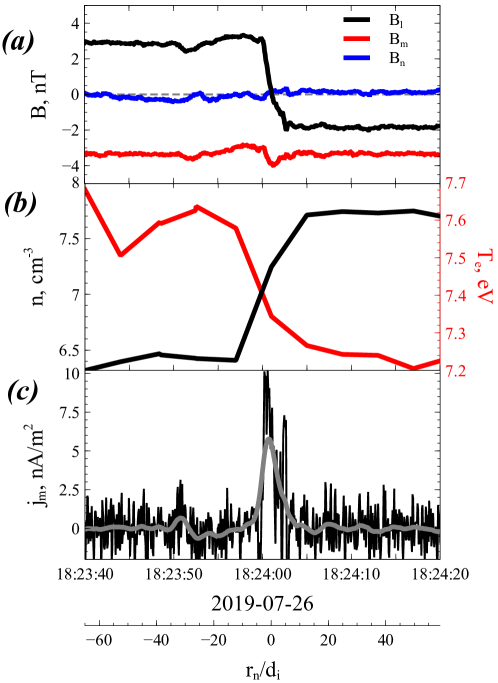
Figure 1: An example of a current sheet crossing by ARTEMIS spacecraft: (a) three magnetic field components in the local coordinate system (Sonnerup & Cahill, 1968) with the additional constraint $\langle B_{n}\rangle=0$ (see section 8.2.6 in Sonnerup & Scheible, 2000), (b) electron density and temperature measurements, (c) current density profile (grey color shows smoothed profile). Bottom horizontal axis show spatial coordinate across the sheet (normalized on the ion inertial length, $d_{i}$).

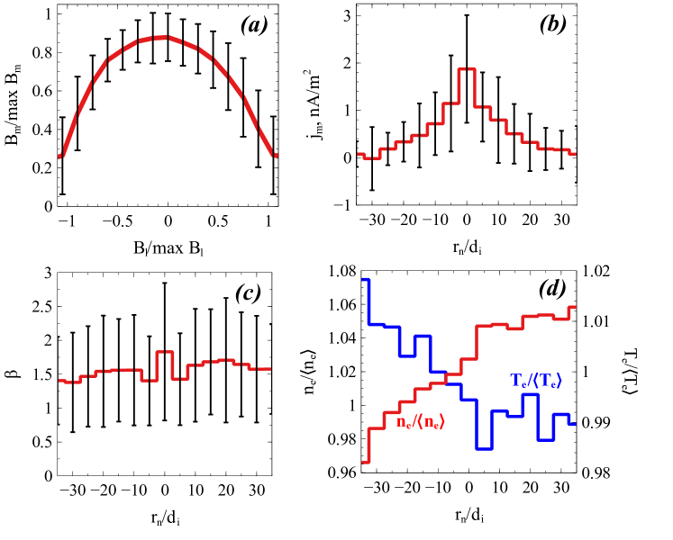
Figure 2: Average profiles of magnetic field, current density, plasma characteristics for a dataset of $\sim 200$ discontinuities observed by the ARTEMIS spacecraft in the near-Earth solar wind (see details of the dataset in Artemyev et al., 2019a). The main criterion of discontinuity selection to the dataset is the peak current density exceeding $1$ nA/m². Black error bars show the standard deviation. In each case, electron densities and temperatures are normalized by the average value across the discontinuity. Orientation of $r_{n}$ is chosen to have $dn_{e}/dr_{n}>0$ for all selected discontinuities.

2 Observations

We present observations of current sheets by the ARTEMIS spacecraft, which probes the solar wind at a few tens of Earth radii upstream of the Earth’s bow shock (Angelopoulos, 2011). We use the magnetic field measurements with temporal resolution of 5 vectors per second (Auster et al., 2008) and measurements of electron density and temperature available at 4s cadence (all plasma parameters are measured by electrostatic analyzers onboard ARTEMIS, see McFadden et al. (2008)).

Figure 1 presents an example of a particular current sheet observed aboard ARTEMIS. Panel (a) presents the magnetic field in the coordinate system (l,m,n) determined using the Minimum Variance Analysis (MVA) (Sonnerup & Cahill, 1968). The magnetic field component $B_{n}$ is perpendicular to the current sheet plane, $B_{l}$ reverses the sign across the current sheet, $B_{m}$ is the so-called guide field. In a 1D approximation all variables vary across the current sheet that is along the normal ${\bf n}$. Panel (a) shows that the current sheet is approximately force-free, because $B_{l}^{2}+B_{m}^{2}\approx{\rm const}$. For the single spacecraft measurements the determination of the normal ${\bf n}$ is generally not sufficiently accurate (e.g., Horbury et al., 2001; Knetter et al., 2004) to separate rotational and tangential discontinuities. Thus, we assume that the observed discontinuity is tangential and apply an additional constraint to the local coordinate system, namely $\langle B_{n}\rangle=0$ (see section 8.2.6 in Sonnerup & Scheible, 2000). Panel (b) shows that the plasma density and electron temperature variations across the current sheet are anti-correlated. The plasma density increases across the current sheet by about 20$\%$, while the electron temperature decreases by about $5\%$. ARTEMIS measurements of the ion temperature in the solar wind are much less accurate than electron temperature measurements. The assumption of the pressure balance across the current sheet suggests that the ion temperature should also decrease across the current sheet by a few tens of percent. Because the Taylor hypothesis applies for the current sheets in the solar wind, we can estimate the current densities $j_{l}\propto-dB_{m}/dt$ and $j_{m}\propto dB_{l}/dt$ (see Artemyev et al., 2019a, for details). Panel (c) shows that the current density reaches values of 10 nA/m², which is comparable to the highest current densities in the solar wind (e.g., Podesta, 2017). The use of the Taylor hypothesis allows translating the observations in time into space. The spatial axis in Figure 1 shows that the current sheet is an ion-scale structure with the thickness of a few ion inertial lengths or, equivalently, a few hundred kilometers. To demonstrate that the current sheet in Figure 1 is not exceptional, we use a dataset of more than four hundred current sheets collected by the ARTEMIS spacecraft over two years of observations (see Artemyev et al., 2019a, for details).

Figure 2 presents the averaged properties of the selected current sheets. Panel (a) shows the current sheets in the solar wind typically have a half-ring $B_{m}$ vs. $B_{l}$. This is equivalent to the statement that ion-scale current sheets in the solar wind are predominantly force-free, i.e. $B_{m}^{2}+B_{l}^{2}\approx{\rm const}$. Panel (b) shows that the $B_{l}$ reversal across the current sheet corresponds to the current density $j_{m}\sim 1$ nA/m² localized within about ten ion inertial lengths. Panel (c) shows that the plasma beta, $\beta=8\pi p/B^{2}$, is typically about unity and does not vary across the current sheets in accordance with the force-free nature of the current sheets. Panel (d) shows that though $\beta$ is approximately uniform across the current sheets, there are clearly variations of the plasma density and electron temperature. Statistically, the plasma density varies by about 10$\%$, while the electron temperature varies by about 3$\%$ across the current sheet.

Although there are kinetic current sheet models that are sufficiently flexible to describe a large variety of tangential discontinuities (see e.g. the review by Roth et al., 1996, and references therein), these models generally require a numerical solution of Maxwell’s equations to achieve self-consistency. This complicates the matching of these models to the observations, in particular with regards to the additional constraints that have to be satisfied by distribution functions for force-free collisionless current sheets. Therefore we will start from a kinetic current sheet model that is completely analytical and already satisfies the force-free condition. However, there are currently no simple analytical kinetic current sheet models which incorporate all of the observed features: (1) the force-free current sheet with spatial scales of a few ion inertial lengths and $\beta$ of the order of unity; (2) anti-correlated plasma density and temperature variations across the current sheet. In the next section we develop kinetic models for such current sheets assuming that they are tangential in nature, that is $B_{n}=0$.

We should mention that not all the discontinuities that were observed (and included in our statistics) are tangential, but that distinguishing observationally between tangential and rotational discontinuities is not a well resolved problem (see discussion in Neugebauer, 2006). The dataset presented in Fig.2 has been collected by the two ARTEMIS probes, whereas at least four-spacecraft observations are required for an accurate determination of the local coordinate system and estimation of $B_{n}$ (Knetter et al., 2004). Therefore, in this paper we focus on modelling tangential discontinuities and leave the question of the relative percentage of tangential versus rotational discontinuities within the total amount of solar wind discontinuities to future investigations.

Independently of the classification of the discontinuities, the observations of these plasma structures in the solar wind are often associated with measurements of plasma shear flow (De Keyser et al., 1998; Paschmann et al., 2013; Artemyev et al., 2019a). This shear flow, which is related to the cross-field plasma (both ion and electron) velocity, can result in the generation of polarization electric fields (e.g., Roth et al., 1996; De Keyser et al., 2013) that are enhanced by plasma pressure gradients across the discontinuities (e.g., Yoon & Lui, 2004; Lu et al., 2019a). However, there are no such gradients in force-free discontinuities. Moreover, some population of these discontinuities have the main magnetic field reversal along solar wind flow, i.e. the plasma shear flow is along the magnetic field and there is almost no cross-field shear flow. For this type of discontinuity the effect of the polarization electric field is negligible. In this paper we will focus on the theoretical description of this type of discontinuity and will not consider a finite electric field. A more general case could, for example, be described in future studies following the approach from De Keyser et al. (2013).

3 Kinetic model of a force-free tangential discontinuity

In this section the local coordinate system $({\bf l},{\bf m},{\bf n})$ is denoted $(x,y,z)$. We consider a one-dimensional current sheet with the magnetic field ${\bf B}=B_{x}(z){\bf e}_{x}+B_{y}(z){\bf e}_{y}$. The development of a stationary kinetic current sheet model requires to provide a class of electron and ion distribution functions $F_{i,e}({\bf v},z)$, which would result in the current density ${\bf j}=j_{x}(z){\bf e}_{x}+j_{y}(z){\bf e}_{y}$ consistent with the magnetic field ${\bf B}$, and the desired spatial distribution of the plasma density and ion and electron temperatures across the current sheet. The particle distribution functions, being solutions of the Vlasov equation, can be written as functions of the integrals of particle motion (e.g., Schindler, 2007). In the considered one-dimensional current sheet there are three integrals of particle motion: the total energy $H_{s}=m_{s}{\bf v}^{2}/2+q_{s}\Phi$ and generalized momenta $p_{xs}=m_{s}v_{x}+q_{s}A_{x}/c$ and $p_{ys}=m_{s}v_{y}+q_{s}A_{y}/c$, where $\Phi(z)$ is the electrostatic potential, ${\bf A}=A_{x}(z){\bf e}_{x}+A_{y}(z){\bf e}_{y}$ is the vector potential, $m_{s}$ and $q_{s}$ are particle mass and charge, $s=i,e$ correspond to ions and electrons ($q_{i}=-q_{e}\equiv e$).

Figure 3 illustrates the macroscopic quantities consistent with the class of kinetic models of force-free current sheets with the magnetic field $B_{x}(z)=B_{0}\tanh(z/L)$ and $B_{y}(z)=B_{0}\cosh^{-1}(z/L)$ developed by Harrison & Neukirch (2009a). In that class of models $B_{x}^{2}+B_{y}^{2}=B_{0}^{2}$, the plasma density and particle temperatures are uniform across the current sheet, and the model parameters are chosen in such a way that the electrostatic field vanishes identically, $\Phi(z)=0$. The plasma $\beta$ is above unity in the original class of Harrison & Neukirch (2009a) models, but $\beta$ can be arbitrary in more generalized models (see Neukirch et al., 2018, for a review). The simplest example from that class of models is the one with the ion distribution function given by the Maxwellian distribution, $F_{0i}({\bf v},z)=n_{0}(m_{i}/2\pi T_{i})^{3/2}\exp(-H_{i}/T_{i})$, and electron distribution function given as follows

$$F_{0e} ({\bf v},z)=n_{0}(1+b)^{-1}\left(\frac{m_{e}}{2\pi T_{e}}\right)^{3/2}\exp(-H_{e}/T_{e})\cdot$$

$$\cdot [b+\exp(u_{0}p_{ye}/T_{e})\exp(-m_{e}u_{0}^{2}/2T_{e})-$$

$$- \frac{1}{2}\cos(u_{0}p_{xe}/T_{e})\exp(m_{e}u_{0}^{2}/2T_{e})],$$

where $n_{0}$ is the plasma density, $T_{e}$ and $T_{i}$ are electron and ion temperatures (here and in the remainder of this paper we absorb the Boltzmann constant factor, $k_{B}$ into the temperature), $u_{0}$ is related to $B_{0}$ and $L$ by the relations $en_{0}u_{0}=-cB_{0}/4\pi L$ and $B_{0}L=-2T_{e}/eu_{0}$. This implies that $L^{2}=cT_{e}/2\pi e^{2}n_{0}u_{0}^{2}$. The electron temperature determines the amplitude of the magnetic field, $B_{0}^{2}=8\pi n_{0}T_{e}$. The parameter $b$ sets the density of the background electron population not contributing to the current density, it has to be large enough to keep the electron velocity distribution function positive. In what follows we generalize the models developed by Harrison & Neukirch (2009a) to have the asymmetric distribution of the plasma density across the current sheet similar to that in Figures 1 and 2.

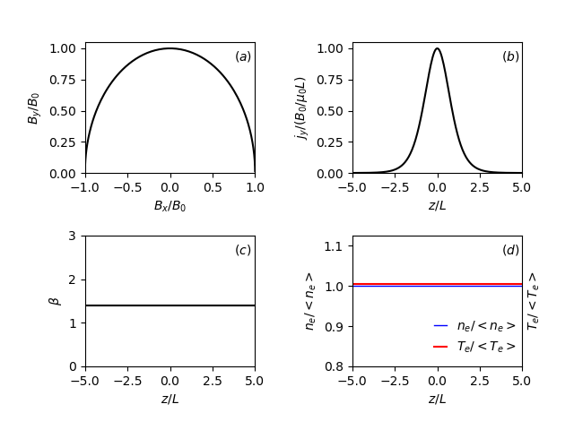
Figure 3: The summary of the macroscopic properties of the current sheet models developed by Harrison & Neukirch (2009b): (a) the half-ring $B_{x}$ vs. $B_{y}$ shape is due to $B_{x}^{2}+B_{y}^{2}=B_{0}^{2}$; (b) the profile of the $y$-component of the current density (c,d) the plasma $\beta$ is generally above unity, while the plasma density and electron and ion temperatures are uniform across the current sheet.

The models of force-free current sheets with asymmetric plasma density profile can be developed within rather wide class of particle velocity distribution functions: $F_{s}=F_{0s}(H_{s},p_{xs},p_{ys})+\Delta F_{s}(H_{s},p_{xs})$, where $F_{0s}$ is, for example, the class of distribution functions suggested by Harrison & Neukirch (2009b), while $\Delta F_{s}(H_{s},p_{xs})$ corresponds to additional electron and ion populations. In principle, $F_{0s}$ can be any distribution function consistent with the magnetic field profile (e.g. Kolotkov et al., 2015; Allanson et al., 2015, 2016; Wilson et al., 2017, 2018). The distribution function of the additional populations should be chosen so that they provide no contribution to the current density, $\int v_{x}\Delta F_{s}d^{3}{\bf v}=0$, but contribute to the density $\int\Delta F_{s}(H_{s},p_{xs})d^{3}{\bf v}=\Delta n_{s}(A_{x})$, where $\Delta n_{s}$ should be an odd function of $A_{x}$ that is $\Delta n_{s}(-A_{x})=-\Delta n_{s}(A_{x})$. In that case the magnetic field remains identical to that in the models of Harrison & Neukirch (2009a), while the electron density distribution will be asymmetric across the current sheet, because $A_{x}(z)=B_{0}L\arctan[\sinh(z/L)]$ is asymmetric with respect to $z=0$. Because the magnetic field configuration remains force-free that is $B^{2}={\rm const}$, the pressure balance across the CS $p_{zz}+B^{2}/8\pi={\rm const}$ results in a constant $zz-$component of the pressure tensor, $p_{zz}={\rm const}$. For a non-uniform plasma density the variation of the temperature $T_{zz}$ across the current sheet is anti-correlated with the density variation.

One of the simplest choices of the velocity distribution functions of the additional populations is $\Delta F_{s}=g_{s}(H_{s})u_{0}p_{xs}/T_{e}$, where $g_{s}(H_{s})$ should satisfy $\int v_{x}^{2}g_{s}(H_{s})d^{3}{\bf v}=0$. The class of functions $g_{s}(H_{s})$ satisfying the latter condition is rather broad, while a particular example is

$$g_{s} = \delta n_{s}\left(\frac{m_{s}}{2\pi T_{s}}\right)^{3/2}\frac{\kappa_{s}^{5/2}e^{-\kappa_{s}H_{s}/T_{s}}-\tilde{\kappa}_{s}^{5/2}e^{-\tilde{\kappa}_{s}H_{s}/T_{s}}}{\kappa_{s}-\tilde{\kappa}_{s}}$$

where $\delta n_{s}$, $\kappa_{s}$ and $\tilde{\kappa}_{s}$ are free parameters. The number of free parameters can be reduced by taking the limit $\tilde{\kappa}_{s}\to\kappa_{s}$, which leads to the following class of $\Delta F_{s}$

$$\Delta F_{s} = \delta n_{s}\left(\frac{\kappa_{s}m_{s}}{2\pi T_{s}}\right)^{3/2}\left(\frac{5}{2}-\frac{\kappa_{s}H_{s}}{T_{s}}\right)e^{-\kappa_{s}H_{s}/T_{s}}\frac{u_{0}p_{xs}}{T_{s}},$$

The additional particle density is given by

$$\Delta n_{s}=-\frac{q_{s}}{e}\delta n_{s}\exp(-q_{s}\kappa_{s}\beta_{s}\Phi)(1-q_{s}\kappa_{s}\beta_{s}\Phi)\frac{2A_{x}}{B_{0}L}.$$ (1)

The quasi-neutrality condition $\sum_{s}q_{s}n_{s}=0$ has the solution $\Phi=0$, if we let $\delta n_{i}=-\delta n_{e}$.

The expression in Eq. (3) is a relatively simple member of a wider class of functions with the desired property that they contribute to the particle density, but not to the current density (if $\Phi=0$). We remark that by choosing parameters appropriately it is always possible to ensure that the total DF, $F_{s}+\Delta F_{s}$, is positive definite.

With $\Phi=0$, $q_{e}=-e$, $q_{i}=e$ (and defining $\delta n_{e}=\epsilon n_{0}$) the additional density term is given by

$$\Delta n_{s}=\Delta n=\epsilon n_{0}\frac{2A_{x}}{B_{0}L}.$$ (2)

Because $A_{x}(z)$ is asymmetric with respect to $z$, $\Delta n_{s}$ introduces the desired density asymmetry across the current sheet. If we define the temperature via the equation $p_{zz,e}=k_{B}T_{e}n_{e}$, the temperature will also be asymmetric due to the pressure remaining constant, as found in the observations (Artemyev et al., 2019b).

In order to construct a realistic example we now assume that $L/d_{i}=10$ (the ratio of the current sheet width to the ion inertial length), $\beta_{p}=1.4$, $T_{e}/T_{i}=1.0$ and $m_{i}/m_{e}=1836$. We then find that $u_{0}/v_{th,e}=\sqrt{2m_{e}/m_{i}\beta_{p}}d_{i}/L\approx-3.9\cdot 10^{-3}$. Using $\kappa_{e}=\kappa_{i}=1.1$ and $\epsilon=0.05$, both distribution functions can be shown to be positive. We show example plots of the variation of the full electron and the ion distribution functions with $v_{x}$ (for fixed values of $z$, $v_{y}$ and $v_{z}$) in Figs. 4 and 5. Due to the relatively small value of $u_{0}/v_{th,e}$, the difference between the total electron and ion distribution functions is also very small. In the same figures we also show how $\Delta F_{s}$ varies with $v_{x}$.

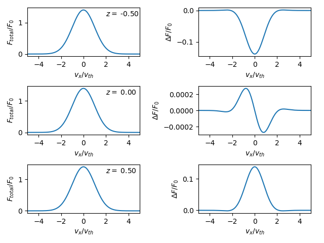
Figure 4: In the left column the dependence of the total electron DF $F_{0e}+\Delta F_{e}$ on $v_{x}$ (for $v_{y}=v_{z}=0$) is shown at three different positions: $z/L=-0.5$ (top row), $z/L=0.0$ (middle row) and $z/L=0.5$ (bottom row). The right column shows the same plots for $\Delta F_{e}$ alone. Here $\epsilon=0.05$ and $u_{0}/v_{th,e}=-3.9\cdot 10^{-3}$.

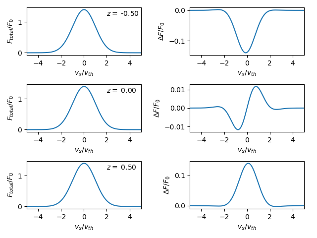
Figure 5: The same plots as in Fig. 4, but for the ions. The only noticeable difference to the plots for the electrons is the larger amplitude of $\Delta F_{i}$ at $z=0$ and the symmetry reversal of its minimum and maximum values.

In Fig. 6 we show the resulting modified density and temperature profiles for the same parameter values that were used for the distribution function plots. As desired the density and temperature profiles show the general behaviour that is also seen in the observation shown in Fig. 2

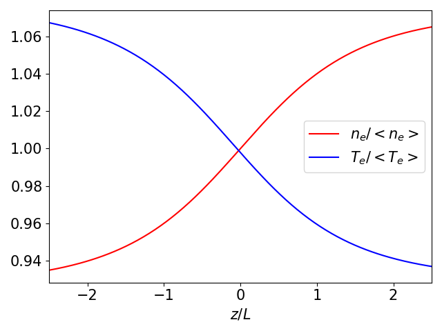
Figure 6: An example of asymmetric density and temperature profiles resulting from the theoretical models ($\epsilon=0.05$).

The structure of the distribution function in velocity space is seen to be very close to a Maxwellian distribution function (see Fig. 4 and Fig. 5). This structure suggests that the distribution functions presented in this paper are likely to be stable to small perturbations (e.g. see standard stability arguments by Gardner, 1963; Krall & Trivelpiece, 1973).

4 Discussion and Conclusion

Recent spacecraft observations have shown that current sheets in the solar wind frequently exhibit non-symmetric and anti-correlated electron density and temperature distributions with respect to the current sheet center (Artemyev et al., 2018). The origin and effects of these features on the stability of the current sheets in the solar wind remains unknown, partly due to absence of kinetic models that could be used in the stability analysis. Self-consistent kinetic models of force-free current sheets have only been developed relatively recently (e.g Harrison & Neukirch, 2009a) and in these models the plasma and temperature distributions are uniform.

In this paper we have demonstrated that by adding a suitable further term to the distribution function of Harrison & Neukirch (2009a) it is possible to generate self-consistent kinetic equilibria which have asymmetric spatial profiles of particle density and temperature, while retaining the macroscopic current sheet equilibrium unchanged. We have presented an illustrative example which showed that for parameter values which are typical for solar wind current sheets observed at 1 A.U., one can easily find self-consistent particle distributions functions giving rise to macroscopic spatial variations in particle density and temperature that closely resemble those found in the observations.

The work presented in this paper could be further extended in a number of ways. For example, instead of using the distribution functions of Harrison & Neukirch (2009a) as $F_{0s}$, one can in principle choose any other particle distribution function giving rise to the same magnetic field profile. While the distribution functions used for $F_{0s}$ in this paper always lead to an equilibrium with plasma $\beta>1$ as well as spatially constant density and temperature profiles, other distribution functions allow for values of plasma $\beta<1$ (e.g. Allanson et al., 2015, 2016; Wilson et al., 2018) or for additional symmetric variations in the particle density and temperature (e.g. Kolotkov et al., 2015).

Another possible extension of the work presented here relates to the specific and relatively simple form for $\Delta F_{s}$ that we have used. This form for $\Delta F_{s}$ is just one example taken from a family of possible $\Delta F_{s}$; other examples include $\Delta F_{s}\propto\sin(K_{s}p_{xs})g_{s}(H_{s})$ and $\Delta F_{s}\propto\exp(K_{s}p_{xs})g_{s}(H_{s})$ (with $\int v_{x}^{2}g_{s}(H_{s})d^{3}{\bf v}=0$ and $K_{s}$ a model dependent constant).

It is also important to point out that within the same class of particle velocity distribution functions one can develop models of force-free current sheets with symmetric density profiles having either maximum or minimum in center of the current sheet (similar to models of Kolotkov et al. (2015)). The symmetric profiles of the plasma density are obtained for distribution functions for which $\Delta n_{s}(A_{x})$ is an even function of $A_{x}$. The additional population should not contribute to the current density and the simplest choice of such particle distribution functions is $\Delta F_{s}=g_{s}(H_{s})(\beta_{e}u_{0}p_{xs})^{2}$, where $g_{s}(H_{s})$ should again satisfy the condition $\int v_{x}^{2}g_{s}(H_{s})d^{3}{\bf v}=0$. For the example distribution function given above, using the same $g_{s}(H_{s})$ that was used in section 3 the plasma density is as $n_{s}=n_{0}(1+\epsilon 4A_{x}^{2}/B_{0}^{2}L^{2})$. As $A_{x}(z)$ is an odd function of $z$, $A^{2}_{x}(z)$ is an even function of $z$ and the density profile is symmetric with respect to the current sheet center.

The self-consistent kinetic current sheet models presented here could, for example, be used as initial conditions for future analyses of collisionless kinetic processes involving tangential discontinuities in the solar wind plasma.

References

- Allanson et al. (2016) Allanson, O., Neukirch, T., Troscheit, S., & Wilson, F. 2016, Journal of Plasma Physics, 82, 905820306
- Allanson et al. (2015) Allanson, O., Neukirch, T., Wilson, F., & Troscheit, S. 2015, Physics of Plasmas, 22, 102116
- Allanson et al. (2018) Allanson, O., Troscheit, S., & Neukirch, T. 2018, IMA Journal of Applied Mathematics, 83, 849
- Angelopoulos (2011) Angelopoulos, V. 2011, Space Sci. Rev., 165, 3
- Angelopoulos et al. (2019) Angelopoulos, V., Cruce, P., Drozdov, A., et al. 2019, Space Sci. Rev., 215, 9
- Artemyev (2011) Artemyev, A. V. 2011, Physics of Plasmas, 18, 022104
- Artemyev et al. (2018) Artemyev, A. V., Angelopoulos, V., Halekas, J. S., et al. 2018, ApJ, 859, 95
- Artemyev et al. (2019a) Artemyev, A. V., Angelopoulos, V., & Vasko, I.-Y. 2019a, J. Geophys. Res., 124, doi:10.1029/2019JA026597
- Artemyev et al. (2019b) Artemyev, A. V., Angelopoulos, V., Vasko, I.-Y., et al. 2019b, Geophys. Res. Lett., 46, 1185–1194
- Auster et al. (2008) Auster, H. U., Glassmeier, K. H., Magnes, W., et al. 2008, Space Sci. Rev., 141, 235
- Bobrova & Syrovatskiǐ (1979) Bobrova, N. A., & Syrovatskiǐ, S. I. 1979, Soviet Journal of Experimental and Theoretical Physics Letters, 30, 567
- Burlaga et al. (1977) Burlaga, L. F., Lemaire, J. F., & Turner, J. M. 1977, J. Geophys. Res., 82, 3191
- Cranmer et al. (2009) Cranmer, S. R., Matthaeus, W. H., Breech, B. A., & Kasper, J. C. 2009, ApJ, 702, 1604
- De Keyser et al. (2013) De Keyser, J., Echim, M., & Roth, M. 2013, Annales Geophysicae, 31, 1297
- De Keyser & Roth (1997) De Keyser, J., & Roth, M. 1997, in ESA Special Publication, Vol. 415, Correlated Phenomena at the Sun, in the Heliosphere and in Geospace, ed. A. Wilson, 75
- De Keyser et al. (1996) De Keyser, J., Roth, M., Lemaire, J., et al. 1996, Sol. Phys., 166, 415
- De Keyser et al. (1998) De Keyser, J., Roth, M., & Söding, A. 1998, Geophys. Res. Lett., 25, 2649
- De Keyser et al. (1997) De Keyser, J., Roth, M., Tsurutani, B. T., Ho, C. M., & Phillips, J. L. 1997, A&A, 321, 945
- Franci et al. (2017) Franci, L., Cerri, S. S., Califano, F., et al. 2017, ApJ, 850, L16
- Gardner (1963) Gardner, C. S. 1963, The Physics of Fluids, 6, 839
- Gosling (2012) Gosling, J. T. 2012, Space Sci. Rev., 172, 187
- Greco et al. (2009) Greco, A., Matthaeus, W. H., Servidio, S., Chuychai, P., & Dmitruk, P. 2009, ApJ, 691, L111
- Greco et al. (2016) Greco, A., Perri, S., Servidio, S., Yordanova, E., & Veltri, P. 2016, ApJ, 823, L39
- Harris (1962) Harris, E. 1962, Nuovo Cimento, 23, 115
- Harrison & Neukirch (2009a) Harrison, M. G., & Neukirch, T. 2009a, Physical Review Letters, 102, 135003
- Harrison & Neukirch (2009b) —. 2009b, Physics of Plasmas, 16, 022106
- Horbury et al. (2001) Horbury, T. S., Burgess, D., Fränz, M., & Owen, C. J. 2001, Geophys. Res. Lett., 28, 677
- Knetter et al. (2004) Knetter, T., Neubauer, F. M., Horbury, T., & Balogh, A. 2004, J. Geophys. Res., 109, A06102
- Kocharovsky et al. (2010) Kocharovsky, V. V., Kocharovsky, V. V., & Martyanov, V. J. 2010, Physical Review Letters, 104, 215002
- Kolotkov et al. (2015) Kolotkov, D. Y., Vasko, I. Y., & Nakariakov, V. M. 2015, Physics of Plasmas, 22, 112902
- Krall & Trivelpiece (1973) Krall, N. A., & Trivelpiece, A. W. 1973, Principles of plasma physics (McGraw-Hill)
- Lemaire & Burlaga (1976) Lemaire, J., & Burlaga, L. F. 1976, Ap&SS, 45, 303
- Lepping (1986) Lepping, R. P. 1986, Advances in Space Research, 6, 269
- Lu et al. (2019a) Lu, S., Artemyev, A. V., Angelopoulos, V., et al. 2019a, J. Geophys. Res., sumbitted
- Lu et al. (2019b) Lu, S., Angelopoulos, V., Artemyev, A. V., et al. 2019b, ApJ, 878, 109
- Mallet et al. (2017) Mallet, A., Schekochihin, A. A., & Chandran, B. D. G. 2017, MNRAS, 468, 4862
- McFadden et al. (2008) McFadden, J. P., Carlson, C. W., Larson, D., et al. 2008, Space Sci. Rev., 141, 277
- Medvedev et al. (1997) Medvedev, M. V., Diamond, P. H., Shevchenko, V. I., & Galinsky, V. L. 1997, Physical Review Letters, 78, 4934
- Neugebauer (2006) Neugebauer, M. 2006, J. Geophys. Res., 111, A04103
- Neukirch et al. (2018) Neukirch, T., Wilson, F., & Allanson, O. 2018, Plasma Physics and Controlled Fusion, 60, 014008
- Neukirch et al. (2009) Neukirch, T., Wilson, F., & Harrison, M. G. 2009, Physics of Plasmas, 16, 122102
- Osman et al. (2011) Osman, K. T., Matthaeus, W. H., Greco, A., & Servidio, S. 2011, ApJ, 727, L11
- Panov et al. (2011) Panov, E. V., Artemyev, A. V., Nakamura, R., & Baumjohann, W. 2011, J. Geophys. Res., 116, A12204
- Paschmann et al. (2013) Paschmann, G., Haaland, S., Sonnerup, B., & Knetter, T. 2013, Annales Geophysicae, 31, 871
- Sonnerup & Scheible (2000) Sonnerup, B. U. Ö., & Scheible, M. 2000, ESA Special Publication, Vol. 449, ISSI Book on Analysis Methods for Multi-Spacecraft Data, ed. G.Paschmann and Patrick W. D.
- Podesta (2017) Podesta, J. J. 2017, J. Geophys. Res., 122, 2795
- Pucci et al. (2018) Pucci, F., Velli, M., Tenerani, A., & Del Sarto, D. 2018, Physics of Plasmas, 25, 032113
- Pulupa et al. (2014) Pulupa, M. P., Salem, C., Phan, T. D., Gosling, J. T., & Bale, S. D. 2014, ApJ, 791, L17
- Roth et al. (1996) Roth, M., De Keyser, J., & Kuznetsova, M. M. 1996, Space Science Reviews, 76, 251
- Schindler (2007) Schindler, K. 2007, Physics of Space Plasma Activity (Cambridge University Press)
- Sonnerup & Cahill (1968) Sonnerup, B. U. Ö., & Cahill, Jr., L. J. 1968, J. Geophys. Res., 73, 1757
- Tsurutani & Smith (1974) Tsurutani, B. T., & Smith, E. J. 1974, J. Geophys. Res., 79, 118
- Tsurutani & Smith (1979) —. 1979, J. Geophys. Res., 84, 2773
- Vasko et al. (2014) Vasko, I. Y., Artemyev, A. V., Petrukovich, A. A., & Malova, H. V. 2014, Annales Geophysicae, 32, 1349
- Vech et al. (2018) Vech, D., Mallet, A., Klein, K. G., & Kasper, J. C. 2018, ApJ, 855, L27
- Wilson & Neukirch (2011) Wilson, F., & Neukirch, T. 2011, Physics of Plasmas, 18, 082108
- Wilson et al. (2017) Wilson, F., Neukirch, T., & Allanson, O. 2017, Physics of Plasmas, 24, 092105
- Wilson et al. (2018) —. 2018, Journal of Plasma Physics, 84, 905840309
- Wilson et al. (2016) Wilson, F., Neukirch, T., Hesse, M., Harrison, M. G., & Stark, C. R. 2016, Physics of Plasmas, 23, 032302
- Yoon & Lui (2004) Yoon, P. H., & Lui, A. T. Y. 2004, J. Geophys. Res., 109, 11213