Spherically symmetric black holes with electric and magnetic charge in extended gravity:
Physical properties, causal structure, and stability analysis in Einstein’s and Jordan’s frames

Abstract

Novel static black hole solutions with electric and magnetic charges are derived for the class of modified gravities: $f({\mathcal{R}})={\mathcal{R}}+2\beta\sqrt{{\mathcal{R}}}$, with or without a cosmological constant. The new black holes behave asymptotically as flat or (A)dS space-times with a dynamical value of the Ricci scalar given by $R=\frac{1}{r^{2}}$ and $R=\frac{8r^{2}\Lambda+1}{r^{2}}$, respectively. They are characterized by three parameters, namely their mass and electric and magnetic charges, and constitute black hole solutions different from those in Einstein’s general relativity. Their singularities are studied by obtaining the Kretschmann scalar and Ricci tensor, which shows a dependence on the parameter $\beta$ that is not permitted to be zero. A conformal transformation is used to display the black holes in Einstein’s frame and check if its physical behavior is changed w.r.t. the Jordan one. The thermal stability of the solutions is discussed by using thermodynamical quantities, in particular the entropy, the Hawking temperature, the quasi-local energy, and the Gibbs free energy. Also, the casual structure of the new black holes is studied, and a stability analysis is performed in both frames using the odd perturbations technique and the study of the geodesic deviation. It is concluded that, generically, there is coincidence of the physical properties of the novel black holes in both frames, although this turns not to be the case for the Hawking temperature.

I Introduction

The discovery of gravitational waves (GW) has shed light on a new possibility to probe the laws of physics in strong gravitational fields Abbott et al. (2016a). General relativity (GR) has been confirmed to a very good precision on weak gravitational field backgrounds Will (2014); however, the precise form of the anticipated, necessary modification of GR to deal with strong gravitational fields is not confirmed yet, although different possibilities have been proposed. The discovery of GW definitely provides an excellent chance to test those modified gravity theories in the strong gravitational fields of black hole solutions Abbott et al. (2016b) and neutron stars Abbott et al. (2017).

The simplest generalizations of GR are the $f({\mathcal{R}})$ gravitational theories, whose Lagrangian involves nonlinear terms in ${\mathcal{R}}$. A simple possibility is power-law gravity, described by a Lagrangian of the form

$$f({\mathcal{R}})={\mathcal{R}}+\frac{{\mathcal{R}}^{n}}{6m^{2}},$$

where $n$ is an arbitrary number and with $m^{2}$ being a positive mass squared. The term ${\mathcal{R}}^{2}$ has a natural interpretation as corresponding to the lowest order quantum perturbative additions to classical gravity, and it is, at the same time, responsible for the inflation at early epoch. In addition, this term should be seriously considered when dealing with local objects on the background of a strong gravitational field. related to this, a numerous of research papers have been focused on the study of black hole solutions, as e.g. Lü et al. (2017); de la Cruz-Dombriz et al. (2009); Nelson (2010); Nojiri and Odintsov (2017, 2013); Kehagias et al. (2015); Cañate et al. (2016); Yu et al. (2018); Cañate (2018); Sultana and Kazanas (2018), and neutron stars solutions Cooney et al. (2010); Arapoglu et al. (2011); El Hanafy and Nashed (2016); Orellana et al. (2013); Awad et al. (2017); Astashenok et al. (2013); Shirafuji and Nashed (1997); Nashed and El Hanafy (2017); Ganguly et al. (2014); Nashed (2011); Capozziello et al. (2016); Nashed and Bamba (2018); Aparicio Resco et al. (2016); Nashed (2014). We should note that $f({\mathcal{R}})$ theories can be related with theories of Brans-Dicke type (see, e.g., Brans and Dicke (1961)), in particular with the ones involving a scalar and a potential of gravitational origin O’Hanlon (1972); Chiba (2003). Similar to what happens with black holes, in Brans-Dicke theories involving a potential with a squared positive mass, a “no-hair (B theorem)” holds, preventing the appearance of non-trivial scalar hair Hawking (1972); Bekenstein (1995). The same theorem forbids the existence of hairy black hole solutions in the case of the ${\mathcal{R}}^{2}$ model de la Cruz-Dombriz et al. (2009); Nelson (2010); Yu et al. (2018); Cañate (2018). Several black holes have been got already for $f({\mathcal{R}})$ theories de la Cruz-Dombriz et al. (2009); Nashed (2018); Moon et al. (2011); Nashed (2018a); Rodrigues et al. (2016); Nashed (2018b); Cañate et al. (2016); Moon and Myung (2011); Ayon-Beato et al. (2010); Hendi et al. (2012, 2014); Cao et al. (2013). And their physical properties are discussed in, e.g., Addazi (2017); Fan and Lü (2015); Akbar and Cai (2007); Faraoni (2010).

The observation of the mathematical similarity between gravitational and electromagnetic fields goes back at least to the eighteenth century, when Coulomb constructed his inverse square law to formulate the force between two charges at a distance $r$ Griffiths (2013). Coulomb’s law is, in this sense, a complete analogue of the gravitational law Newton (1687) for the force acting on two masses separated by the same distance. The similarity between this expression for the two forces led scientists to conjecture that the gravitational force exerted by the sun on the planets could be accompanied by a magnetic force leading to the precession of their orbits and, thence, they would investigate from this standpoint the discrepancy found by Newton in the precession of Mercury’s orbit. In fact, Mercury’s perihelion precession was definitely explained by Einstein’s GR, sometime after this similarity between gravitational and electromagnetic fields had been exploited, in some regimes. Moreover, it is known that gravitation involves a gravitomagnetic field because of the mass current Thirring (1918); Lense and Thirring (1918, 1918); CIUFOLINI and WHEELER (1995). Additionally, Einstein GR forecasts a gravitomagnetic field because of the proper rotation of the Sun that effects the planetary orbits Mashhoon et al. (1984); de Sitter (1916); Dass and Liberati (2019). Those are well-known facts. The aim of the present paper is to construct brand new black hole solutions, possessing electric and magnetic charge, within the family of $f({\mathcal{R}})$ modified gravities, to describe them in both the Jordan and the Einstein frames, and to study a number of their physical properties, by calculating associated thermodynamical quantities. Moreover, we will study their causal structure and perform a detailed stability analysis by using odd perturbation techniques and the study of the geodesic deviation.

The formulation of this study is as follows. A brief introduction to the theory of Maxwell-$f({\mathcal{R}})$ gravity is given in Sec. II. In Sec. III, restricting to spherical symmetry, an exact solution of the field equations of the Maxwell-$f({\mathcal{R}})$ theory is obtained. In Sec. IV, the same derivation is performed for the case of the Maxwell-$f({\mathcal{R}})$ theory involving a cosmological constant. We obtain a novel solution which asymptotically has AdS or dS space. We discuss in detail the characteristic features of these solutions in Sec. V. In Sec. VI, by using conformal transformation, we derive the black hole solutions in the Einstein frame. In Sec. VII, basic thermodynamical quantities, such as the entropy, quasi-local energy, the Hawking temperature, and the Gibbs energy are calculated in both the Einstein and the Jordan frames. These calculations show that (with the sole exception of the Hawking temperature) the physical behavior of the black holes obtained do not change generically in going from one to the other frame. Using the odd perturbations technique, the analysis of the linear stability of the solutions obtained in Secs. III, IV and VI is performed in Sec. VIII. Stability conditions, in relation with geodesic motion are obtained in Sec. IX. And the causal structure of the solution derived in Sec. III is discussed in Sec. X. Finally, in Sec. XI we present a summary of the main results of this work, draw some compelling conclusions, and discuss some ideas for future work.

II Brief note on the Maxwell–$f({\mathcal{R}})$ theory

The theory of $f({\mathcal{R}})$ gravity is an extension of Einstein’s GR, first discussed in Buchdahl (1970); Capozziello and De Laurentis (2011); Nojiri and Odintsov (2011); Nojiri et al. (2017); Capozziello et al. (2003); Capozziello (2002); Nojiri and Odintsov (2003); Carroll et al. (2004). The Lagrangian of this theory is

$${\mathop{\mathcal{L}}}:={\mathop{\mathcal{L}}}_{g}+{\mathop{\mathcal{L}}}_{E.M.},$$ (1)

its gravitational term being ${\mathop{\mathcal{L}}}_{g}$, which is given by

$${\mathop{\mathcal{L}}}_{g}:=\frac{1}{2\kappa}\int d^{4}x\sqrt{-g}(f({\mathcal{R}})-\Lambda).$$ (2)

Here ${\mathcal{R}}$ represents the Ricci scalar, $\kappa$ is the Newtonian constant, $\Lambda$ is the cosmological constant, $g$ the metric determinant, and $f({\mathcal{R}})$ a certain analytic function. Here, we have defined the energy-momentum as ${\mathop{\mathcal{L}}}_{{}_{{}_{E.M.}}}$, the Lagrangian of the electromagnetic field, which is given by

$${\mathop{\mathcal{L}}}_{{}_{{}_{E.M.}}}:=-\frac{1}{2}F^{2},$$ (3)

where $F^{2}=F_{\mu\nu}F^{\mu\nu}$ and $F_{\mu\nu}=2\xi_{[\mu,\nu]}$, where $\xi_{\mu}$ is the gauge potential and comma refers to the ordinary differentiation Hendi and Momeni (2011).

Performing the variations of the Lagrangian of Eq. (1) w.r.t. the metric tensor $g_{\mu\nu}$ and w.r.t. the strength tensor $F$, respectively, one gets the field equations of the Maxwell-$f({\mathcal{R}})$ theory, in the form Cognola et al. (2005)

$$\zeta_{\mu\nu}={\mathcal{R}}_{\mu\nu}f_{\mathcal{R}}-\frac{1}{2}g_{\mu\nu}f({\mathcal{R}})-2g_{\mu\nu}\Lambda+g_{\mu\nu}\Box f_{\mathcal{R}}-\nabla_{\mu}\nabla_{\nu}f_{\mathcal{R}}-8\pi T_{\mu\nu}\equiv 0,$$ (4)

$$\partial_{\nu}\left(\sqrt{-g}{\textrm{F}}^{\mu\nu}\right)=0,$$ (5)

where ${\mathcal{R}}_{\mu\nu}$ is the Ricci tensor and $\Box$ is the d’Alembertian operator, $\nabla_{\alpha}A^{\beta}$ is the covariant derivative of the vector $A^{\beta}$, and ${\displaystyle f_{\mathcal{R}}=\frac{df({\mathcal{R}})}{d{\mathcal{R}}}}$. Here, we define the energy-momentum tensor, $T_{\mu\nu}$, as

$$T_{\mu\nu}:=\frac{1}{4\pi}\left({\textrm{g}}_{\rho\sigma}{{\textrm{F}}_{\nu}{}^{\rho}}{{{\textrm{F}}}_{\mu}}^{\sigma}-\displaystyle{1\over 4}{\textrm{g}}_{\mu\nu}F^{2}\right).$$ (6)

Taking the trace in Eq. (4), one gets

$$\zeta={\mathcal{R}}f_{\mathcal{R}}-2f({\mathcal{R}})-8\Lambda+3\Box f_{\mathcal{R}}=0\,.$$ (7)

Now, we shall take a specific form for the field Eqs. (4), both with and without a cosmological constant to derive exact charged black holes, which behave asymptotically as AdS/dS or flat space-times, respectively.

III Black hole solutions with magnetic and electric charge

In this section, we are going to derive a charged black hole for the following specific model

$$f({\mathcal{R}})={\mathcal{R}}+2\beta\sqrt{{\mathcal{R}}}.$$ (8)

To achieve this, we introduce the following spherically symmetric ansatz

$$ds^{2}=-w(r)dt^{2}+\frac{dr^{2}}{w(r)}+r^{2}(d\theta^{2}+\sin^{2}d\phi^{2}).$$ (9)

The Ricci scalar of the line-element (9) is given by

$${\mathcal{R}}=\frac{2-r^{2}w^{\prime\prime}-4rw^{\prime}-2w}{r^{2}},$$ (10)

where $w\equiv w(r)$, $w^{\prime}\equiv\frac{dw(r)}{dr}$, and $w^{\prime\prime}\equiv\frac{d^{2}w(r)}{dr^{2}}$. Using Eqs. (9) in (4), (5) and (7), after using Eq. (10) we get a system of fourth order differential equations which are listed in Appendix A. The off-diagonal components of these system, $(A\cdot 2)$, $(A\cdot 4)$ and $(A\cdot 5)$, can be solved to determine the unknown functions $n$, $p$, $s$, and $k$. Substituting the values of these function into the diagonal components, as well as into the trace field equation, we obtain

$$w(r)=\frac{1}{2}+\frac{c_{1}}{r}+\frac{{q_{{}_{E}}}{}^{2}+{q_{{}_{M}}}{}^{2}}{r^{2}},\qquad q=\frac{{q_{{}_{E}}}}{r},\qquad n=c_{2}\theta,\qquad s=c_{2}r,\qquad p=c_{3}r,\qquad k=c_{4}\theta-{q_{{}_{M}}}\cos\theta,$$ (11)

where the $c_{i}$, $i=1\cdots 4$, are constant, and $q_{{}_{E}}$ and $q_{{}_{M}}$ are other constants related to the electric and magnetic charge, respectively. The analytic solution (11) satisfies the system of differential equations presented in Appendix A, including the trace of the field equations, provided that $c_{1}=\frac{1}{3\beta}$. The Ricci scalar is obtained, in the form

$${\mathcal{R}}=\frac{1}{r^{2}}\,.$$ (12)

This is a consistency check of the procedure, too. The solution (11) metric reads

$$ds^{2}=-\left(\frac{1}{2}+\frac{1}{3\beta r}+\frac{{\mathcal{K}}^{2}}{r^{2}}\right)dt^{2}+\left(\frac{1}{2}+\frac{1}{3\beta r}+\frac{{\mathcal{K}}^{2}}{r^{2}}\right)^{-1}dr^{2}+r^{2}d\Omega^{2},$$ (13)

where we have set ${q_{{}_{E}}}{}^{2}+{q_{{}_{M}}}{}^{2}={\mathcal{K}}^{2}$. Eq. (13) behaves asymptotically as a flat space-time. Solution (11) coincides with that obtained in Sebastiani and Zerbini (2011) when ${\mathcal{K}}^{2}=0$, i.e. $q_{E}=q_{M}=0$. Also, the solution obtained (13) corresponds to the spherically symmetric space-time in $f({\mathcal{R}})$ gravitational theories, and differs from the corresponding one in Nashed and Capozziello (2019) by the more general expression of the 1-form gauge potential, given in Eq. $(A\cdot 9)$, and by the parameter ${\mathcal{K}}$ that couples to electric and magnetic fields.

IV Analytic AdS/dS charged solutions

In order to obtain a black hole solution with charge, behaving asymptotically as AdS/dS, we take $f(R)$ of the form

$$f({\mathcal{R}})={\mathcal{R}}+2\beta\sqrt{{\mathcal{R}}-8\Lambda}.$$ (14)

Using now the anzatz (9) in the field Eqs. (4), (5), and (7), and after applying (10), we obtain a system of fourth order differential equations listed in Appendix B.

Using the previous procedure, namely solving the off-diagonal components and substituting their values in the diagonal ones, we get the following exact solution

$$w(r)=\frac{1}{2}-\frac{2r^{2}\Lambda}{3}+\frac{1}{3\beta r}+\frac{{q_{{}_{E}}}{}^{2}+{q_{{}_{M}}}{}^{2}}{r^{2}},\qquad q=\frac{{q_{{}_{E}}}}{r},\qquad n=c_{2}\theta,\qquad s=c_{2}r,\qquad p=c_{3}r,\qquad k=c_{4}\theta-{q_{{}_{M}}}\cos\theta.$$ (15)

Introducing Eq. (15) into (10), we obtain the Ricci scalar, as follows

$${\mathcal{R}}=\frac{8r^{2}\Lambda+1}{r^{2}}.$$ (16)

The solution (15) metric reads

$$ds^{2}=-\left(\frac{1}{2}-\frac{2r^{2}\Lambda}{3}+\frac{1}{3\beta r}+\frac{{q_{{}_{E}}}{}^{2}+{q_{{}_{M}}}{}^{2}}{r^{2}}\right)dt^{2}+\left(\frac{1}{2}-\frac{2r^{2}\Lambda}{3}+\frac{1}{3\beta r}+\frac{{q_{{}_{E}}}{}^{2}+{q_{{}_{M}}}{}^{2}}{r^{2}}\right)^{-1}dr^{2}+r^{2}d\Omega^{2}\,,$$ (17)

and behaves asymptotically as AdS/dS space-time. The solution (15) is different from the one derived in Sebastiani and Zerbini (2011), owing to the same reason already discussed for the solution (11).

V Properties of the found black holes

For the solution (11), the metric can be put as

$$ds^{2}=-\left(\frac{1}{2}-\frac{m}{r}+\frac{{\mathcal{K}}^{2}}{r^{2}}\right)dt^{2}+\left(\frac{1}{2}-\frac{m}{r}+\frac{{\mathcal{K}}^{2}}{r^{2}}\right)^{-1}dr^{2}+r^{2}d\Omega^{2}\;,\qquad\textrm{where}\qquad m=-c_{1}=-\frac{1}{3\beta}.$$ (18)

Eq. (18) indicates that the dimensional parameter $\beta$ cannot vanish. And this says that the line-element is the same as for Reissner-Nordström space-time when ${\mathcal{K}}=q_{{}_{E}}$ and $q_{{}_{M}}=0$.

The line-element of the solution (15) can be written as

$$ds^{2}=\left(\frac{1}{2}-\frac{2r^{2}\Lambda}{3}-\frac{m}{r}+\frac{{\mathcal{K}}^{2}}{r^{2}}\right)dt^{2}-\left(\frac{1}{2}-\frac{2r^{2}\Lambda}{3}-\frac{m}{r}+\frac{{\mathcal{K}}^{2}}{r^{2}}\right)^{-1}dr^{2}-r^{2}d\Omega^{2}\;,\qquad\textrm{where, again}\qquad m=-c_{1}=-\frac{1}{3\beta},$$ (19)

which tells us that the line-element (19) does behave asymptotically as AdS/dS and that it coincides with the Reissner-Nordström space-time when ${\mathcal{K}}=q_{{}_{E}}$ and $q_{{}_{M}}=0$. Eqs. (18) and (19) insure that $\beta\neq 0$.

We now turn to the regularity of the solutions (11) and (15), for $w(r)=0$. For (11), we calculate the scalar invariants, with the result

$${\mathcal{R}}^{\mu\nu\lambda\rho}{\mathcal{R}}_{\mu\nu\lambda\rho}=\frac{4r^{2}-4\beta r^{3}+3r^{4}\beta^{2}+{\mathcal{K}}^{2}[48r\beta-12r^{2}\beta^{2}+168\beta^{2}]+336\beta q_{{}_{M}}^{2}q_{{}_{M}}^{2}}{3\beta^{2}r^{8}},$$

$${\mathcal{R}}^{\mu\nu}{\mathcal{R}}_{\mu\nu}=\frac{r^{4}+{\mathcal{K}}^{2}[4r^{2}+8{\mathcal{K}}^{2}]}{2r^{8}},\qquad\qquad{\mathcal{R}}=\frac{1}{r^{2}},$$ (20)

where ${\mathcal{R}}$, ${\mathcal{R}}^{\mu\nu}{\mathcal{R}}_{\mu\nu}$, and ${\mathcal{R}}^{\mu\nu\lambda\rho}{\mathcal{R}}_{\mu\nu\lambda\rho}$ are the Ricci scalar, the Ricci tensor square, and the Kretschmann scalars, respectively. Eqs. (V) show that, at $r=0$, the solutions develop a true singularity in which the dimensional parameter $\beta$ cannot vanish, so that the solution (11) is not reducible to one of GR. Thus, this black hole is a brand new one of the class of $f({\mathcal{R}})$ modified theories.

Employing Eq. (15), we obtain the scalar invariants, as

$${\mathcal{R}}^{\mu\nu\lambda\rho}{\mathcal{R}}_{\mu\nu\lambda\rho}=\frac{4r^{2}-4\beta r^{3}+3r^{4}\beta^{2}+{\mathcal{K}}^{2}[48r\beta-12r^{2}\beta^{2}+168\beta^{2}]+336\beta q_{{}_{M}}^{2}q_{{}_{M}}^{2}+8r^{6}\beta^{2}\Lambda[4r^{2}\Lambda+1]}{3\beta^{2}r^{8}},$$

$${\mathcal{R}}^{\mu\nu}{\mathcal{R}}_{\mu\nu}=\frac{r^{4}+{\mathcal{K}}^{2}[4r^{2}+8{\mathcal{K}}^{2}]+8r^{6}\beta^{2}\Lambda[4r^{2}\Lambda+1]}{2r^{8}},\qquad\qquad\qquad{\mathcal{R}}=\frac{8r^{2}\Lambda+1}{r^{2}}.$$

The same considerations already done for the solution (11) can also be applied now to the solution (15), what will insure also that (15) is a brand new, charged solution constructed in the class of $f({\mathcal{R}})$ gravities, and that it cannot possibly be reduced to a GR solution.

VI Charged black hole solutions in the Einstein frame

In this section we will construct charged black holes in the Einstein frame. We thus start with a brief description of $f(R)$ theories in the Einstein frame. It is rather well-know that $f(R)$ gravitational theories can be rewritten under the form of a Brans-Dicke theory, by involving a subsidiary field, $\psi$, through a non-minimal coupling term, as

$${\mathcal{L}}:=\int d^{4}x\sqrt{-g}\,\left[\frac{1}{2\kappa}f_{\psi}(\psi)(R-\Lambda)-\left(\frac{\psi f_{\psi}(\psi)-f(\psi)}{2\kappa}\right)\right]+{\mathop{\mathcal{L}}}_{{}_{E.M.}},$$ (22)

where $f_{\psi}(\psi)=\frac{f(\psi)}{d\psi}$ and ${\mathop{\mathcal{L}}}_{{}_{E.M.}}$ is the Lagrangian of the electromagnetic field, given by Eq. (3). Variation of Eq. (22) w.r.t. $\psi$ gives $f_{\psi\psi}(R-\Lambda-\psi)=0$. For $f_{\psi\psi}\neq 0$, one can obtain $\psi=R-\Lambda$ and the above action returns back to the one of Eq. (1). This means that the field equations produced by the action (22) exactly coincide with those previously derived from the Lagrangian (1), namely (4) and (5).

When choosing $\sigma=f_{\psi}(\psi)$, the Lagrangian (22) is termed as a Brans–Dicke’s like theory with a non-minimal coupling term $\sigma R$ and a scalaron potential $V(\sigma)$. It is well-know that the non-minimal coupling term can be eliminated from the Jordan frame, by moving to the Einstein frame, using the following conformal transformation

$$g_{\mu\nu}\to{\bar{g}}_{\mu\nu}(x)=\Omega^{2}(x)g_{\mu\nu}(x),$$ (23)

where the space-time conformal factor has been chosen as $\Omega^{2}(x)=f_{\mathcal{R}}$, what demands that $f_{\mathcal{R}}>0$ Bahamonde et al. (2017, 2016). From the transformation (23), one can show that the Ricci scalar transforms as $R\to\bar{R}$. Using now the canonical scalar field

$$\psi=\sqrt{\frac{6}{\kappa}}\,\ln\Omega=\sqrt{\frac{3}{2\kappa}}\,\ln f_{\mathcal{R}},$$ (24)

and from the conformal transformation (23), the Lagrangian (22) converts into a scalar-tensor theory in the Einstein frame, as

$${\mathop{\mathcal{L}_{E}}}:=\int d^{4}x\sqrt{-{\bar{g}}}\left[\frac{1}{2\kappa}({\bar{\mathcal{R}}}-\Lambda)-\frac{1}{2}{{\bar{g}}}^{\mu\nu}\partial_{\mu}\psi\partial_{\nu}\psi-V(\psi)\right]+\mathcal{L}_{{}_{E.M.}},$$ (25)

where

$$V_{E}(\psi)=\displaystyle\frac{{\mathcal{R}}f_{\mathcal{R}}-f}{2\kappa{f_{\mathcal{R}}}^{2}}=\frac{V(\psi)}{f_{R}^{2}},$$ (26)

is the potential of the canonical scalar field $\psi$. The potential $V_{E}(\psi)$ can be rewritten in terms of $\psi$ by using the inverse relation $f_{\mathcal{R}}=e^{\sqrt{2\kappa/3}\,\psi}$. Performing the conformal transformation (23), the energy–momentum tensor converts into Hendi (2010); Bhattacharya and Majhi (2017); Capozziello et al. (2010); Bahamonde et al. (2016); Bamba and Odintsov (2015); Chakraborty et al. (2019)

$$T_{\mu\nu}\to\bar{T}_{\mu\nu}=\Omega(x)^{-2}T_{\mu\nu}.$$ (27)

In the following, we are going to apply the conformal transformation (23) to the space-time metric (18), i.e. $d\bar{s}_{E}^{2}=\Omega^{2}ds_{J}^{2}$, where the conformal factor of the $f(R)$ gravity (8) is given by

$$\Omega^{2}=f_{R}=1+r\beta.$$ (28)

The relation between the scalar field $\Omega$ and the radial coordinate $r$ is plotted in Fig. 1.

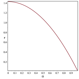
Figure 1: Plot of the radial coordinate, $r$, in terms of the scalar field, $\Omega$

Finally, using Eq. (26), the potential of this model reads

$$V(r)=-\frac{\beta}{2\kappa^{2}r(1+\beta r)^{2}},\Rightarrow V(\Omega)=\frac{\beta^{2}}{2\kappa^{2}\Omega^{4}(1-\Omega^{2})}.$$ (29)

Eq. (29) is plotted in Fig.2.

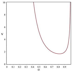
Figure 2: Schematic plot of the scalar field $\Omega$ versus the potential $V$.

Thus, we can write the Einstein frame metric as

$$d\bar{s}_{E}^{2} = \Omega^{2}\left[-w(r)dt^{2}+\frac{dr^{2}}{w(r)}+r^{2}\left(d\theta^{2}+\sin^{2}\theta d\phi^{2}\right)\right],$$ (30)

$$= -\bar{w}(\bar{r})dt^{2}+\frac{d\bar{r}^{2}}{\bar{w_{1}}(\bar{r})}+\bar{r}^{2}\left(d\theta^{2}+\sin^{2}\theta d\phi^{2}\right),$$

where

$$\bar{r}=\Omega(r)r,\qquad\bar{w}(\bar{r})=w(r(\bar{r}))=\Omega^{2}(\bar{r})w(\bar{r}),\quad\bar{w}_{1}(\bar{r})=w_{1}(r(\bar{r}))=\frac{\Omega^{2}(\bar{r})[x^{2}(\bar{r})+12x(\bar{r})+144]^{2}}{16x(\bar{r})[x^{2}(\bar{r})+6x(\bar{r})+144]}\,,\quad\textrm{where}$$

$$x(\bar{r})=\Bigg{\{}12\Big{[}9\beta\bar{r}+\sqrt{81\beta^{2}\bar{r}^{2}-12}\Big{]}\Bigg{\}}^{2/3}.$$ (31)

Eq. (VI) shows that the solutions (11) and (15) have been deformed due to the conformal transformation (23) and that the dimensional parameter $\beta$ must satisfy $\beta>\frac{2}{3\sqrt{3}\bar{r}}$. Is this deformation effect conveying the physics in both the Jordan and the Einstein frames? We will answer this question in the next section.

VII Black hole thermodynamics in the Jordan frame

The Hawking temperature is usually defined as Sheykhi (2012, 2010); Hendi et al. (2010); Sheykhi et al. (2010)

$$T_{+}=\frac{w^{\prime}(r_{+})}{4\pi},$$ (32)

where the event horizon $r=r_{+}$ is the positive solution of the equation $w(r_{+})=0$ which satisfies $w^{\prime}(r_{+})\neq 0$. In the framework of $f({\mathcal{R}})$ gravity, the entropy is given by Cognola et al. (2011); Zheng and Yang (2018)

$$S(r_{+})=\frac{1}{4}Af_{{\mathcal{R}}}(r_{+}),$$ (33)

where $A$ represents the area. The quasi-local energy is defined in the context of $f({\mathcal{R}})$ theory as Cognola et al. (2011); Zheng and Yang (2018)

$$E(r_{+})=\frac{1}{4}\displaystyle{\int}\Bigg{[}2f_{{\mathcal{R}}}(r_{+})+r_{+}{}^{2}\Big{\{}f({\mathcal{R}}(r_{+}))-{\mathcal{R}}(r_{+})f_{{\mathcal{R}}}(r_{+})\Big{\}}\Bigg{]}dr_{+}.$$ (34)

The constraint $w(r_{+})=0$ yields

$${r_{+}}_{{}_{{}_{{}_{{}_{\tiny Eq.(\ref{sol})}}}}}=-\frac{1}{3\beta}\left[1+\sqrt{1-18\beta^{2}{\mathcal{K}}^{2}}\right],\qquad\qquad{r_{-}}_{{}_{{}_{{}_{{}_{\tiny Eq.(\ref{sol})}}}}}=\frac{1}{3\beta}\left[\sqrt{1-18\beta^{2}{\mathcal{K}}^{2}}-1\right],$$

$${r_{+}}_{{}_{{}_{{}_{{}_{\tiny Eq.(\ref{sol1})}}}}}=Root(4y^{4}\beta\Lambda+2y-3\beta y^{2}-6\beta{\mathcal{K}}^{2}),$$ (35)

where $Root(4y^{4}\beta\Lambda-3\beta y^{2}+2y+2)$ are the roots of the equation $(4y^{4}\beta\Lambda+2y-3\beta y^{2}-6\beta{\mathcal{K}}^{2}=0)$, which is proven to have one real root. The first equation of (VII) The first of Eqs. (VII) tells us that the parameter $\beta$ cannot vanish, therefore the solution (11) has no corresponding one in the GR limit. Also, Eq. (VII) indicates that the parameter $\beta$ must be negative, therefore, when there is no charge the horizons have a positive real value. Furthermore, Eq. (VII) also sets constraints on $\beta$, namely $\beta<\frac{1}{3{\mathcal{K}}\sqrt{2}}$. The behavior of the radial coordinate, $r$, in terms of the parameter $\beta$ is plotted in Fig. 32(a). Also, we plot there the behavior of the radial coordinate $r$ and the parameter $\beta$ for the third equation of (VII). We now resume our consideration of the thermodynamics, assuming $\beta<0$, in accordance with the previous discussion, and considering the outer event horizon, $r_{+}$, which agrees with the constraint $\beta<0$.

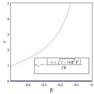
(a)  Spherically symmetric space-time

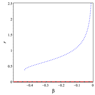
(b)  Spherically symmetric AdS/dS space-times

Figure 3: Plot of $r$ versus $\beta$ for the black holes (11) and (15), respectively.

From Eq. (33), the entropy of solutions (11) and (15) takes the form

$${S_{+}}_{{}_{{}_{{}_{{}_{\tiny Eq.(\ref{sol})}}}}} = \frac{\pi}{27\beta^{2}}\left[1-\sqrt{1-18\beta^{2}{\mathcal{K}}^{2}}\right]^{2}\left[2+\sqrt{1-18\beta^{2}{\mathcal{K}}^{2}}\right],$$

$${S_{+}}_{{}_{{}_{{}_{{}_{\tiny Eq.(\ref{sol1})}}}}} = \frac{\pi r_{+}{}^{2}}{4}\left[1+\beta r_{+}\right].$$ (36)

The first of Eqs. (VII) clearly proves that we have a positive entropy, all the time. The second of Eqs. (VII) indicates that $\beta<-\frac{1}{r_{+}}$, so as to obtain a positive entropy. Eqs. (VII) are represented in Fig. 4. Observe the entropy $S$ not being proportional to $A$, because of Eq. (33). And also that $S$ is in fact proportional to $A$ (as it should) provided of course that $f_{\mathcal{R}}=1$.

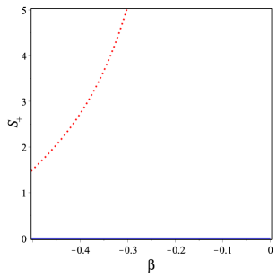
(a)  Plot of the black hole solution’s entropy

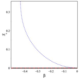
(b)  Plot of the black hole solution’s entropy

Figure 4: Plot of the entropy of the solutions (11) and (15) versus $\beta$.

The Hawking temperatures of solutions (11) and (15) are, respectively,

$${T_{+}}_{{}_{{}_{{}_{{}_{\tiny Eq.(\ref{sol})}}}}} = -\frac{3\beta\left[1-18\beta^{2}{\mathcal{K}}^{2}-\sqrt{1-18\beta^{2}{\mathcal{K}}^{2}}\right]^{2}}{4\pi(1-\sqrt{1-18\beta^{2}{\mathcal{K}}^{2}})^{3}},$$

$${T_{+}}_{{}_{{}_{{}_{{}_{\tiny Eq.(\ref{sol1})}}}}} = -\frac{2\beta[2\Lambda r_{+}{}^{4}+3{\mathcal{K}}^{2}]+r_{+}}{12\pi\beta r_{+}{}^{3}},$$ (37)

with ${T_{+}}$ being the temperature of Hawking’s at the event horizon. We depicted the Hawking’s temperature in Fig. 5. Fig. 5 4(a) proves that we do have a positive temperature for the black hole (11) and also Fig. 5 4(b) shows that the temperature is always positive for the black hole (15).

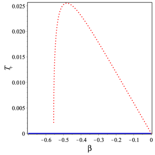
(a)  The black hole solution’s temperature in Jordan’s frame

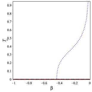
(b)  The black hole solution’s temperature in Jordan’s frame

Figure 5: Plot of the black hole’s temperature in the Jordan frame in terms of the dimensional parameter $\beta$.

From Eq. (34), the quasi-local energy of (11) and (15), is obtained as

$${E_{+}}_{{}_{{}_{{}_{{}_{\tiny Eq.(\ref{sol})}}}}} = -\frac{1+9\beta^{2}{\mathcal{K}}^{2}-\sqrt{1-18\beta^{2}{\mathcal{K}}^{2}}}{12\beta},$$

$${E_{+}}_{{}_{{}_{{}_{{}_{\tiny Eq.(\ref{sol1})}}}}} = \frac{r_{+}}{8}\left(4+3\beta r_{+}\right).$$ (38)

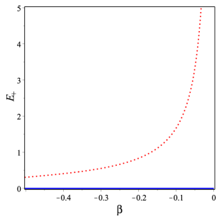
(a)  The black hole’s (11) quasilocal energy

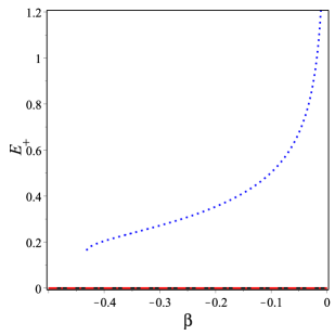
(b)  The black hole’s (15) quasilocal energy

Figure 6: Plot of the black holes quasilocal energy in the Jordan frame versus $\beta$.

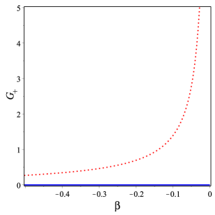
(a)  The black hole’s (11) free energy

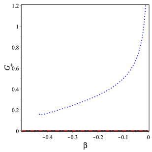
(b)  The black hole’s (15) free energy

Figure 7: Plot of the black hole’s free energy in the Jordan frame versus $\beta$.

From the first of Eqs. (VII) we see that $\beta\neq 0$. The Gibbs free energy is given by Zheng and Yang (2018); Kim and Kim (2012)

$$G(r_{+})=E(r_{+})-T(r_{+})S(r_{+})$$ (39)

where $V$ is the black hole’s geometric volume and $P$ is the pressure, represented by the radial equation of (4), namely $I_{r}{}^{r}$. The quantities $E(r_{+})$, $T(r_{+})$ and $S(r_{+})$ are the quasilocal energy, temperature and entropy at the event horizon, respectively. From Eqs. (VII), (VII) and (VII) in (39), we obtain

$${G_{+}}_{{}_{{}_{{}_{{}_{\tiny Eq.(\ref{sol})}}}}}=\frac{(5+9\beta^{2}{\mathcal{K}}^{2})\sqrt{1-18\beta^{2}{\mathcal{K}}^{2}}-5+9\beta^{2}{\mathcal{K}}^{2}}{36\beta(1-\sqrt{1-18\beta^{2}{\mathcal{K}}^{2}})},$$

$${G_{+}}_{{}_{{}_{{}_{{}_{\tiny Eq.(\ref{sol1})}}}}}=\frac{r_{+}(4+3\beta r_{+})}{8}+\frac{(r_{+}+2\beta[2\Lambda\beta r_{+}{}^{4}+3\beta{\mathcal{K}}^{2}])(1+\beta r_{+})}{12\beta r_{+}}.$$ (40)

In Figs. 76(a), 76(b), the behavior of the black holes’ Gibbs energy is represented for particular values of the parameters of the model.

VII.1 Black hole thermodynamics in Einstein’s frame

In this section we will to repeat the previous calculations but this time in Einstein’s frame, i.e. using Eqs. (VI) to derive the thermodynamics of the black holes and compare them with the corresponding ones in (11) and (15).

The constraint $w(r(\bar{r_{+}}))=0$ for the flat and AdS/Ad cases gives

$${\bar{r}}_{+}{}_{{}_{{}_{{}_{{}_{\tiny Eq.(\ref{sol})}}}}}=-\frac{\sqrt{6}}{18\beta(2\sqrt{36\beta^{2}{\mathcal{K}}^{2}+324\beta^{4}{\mathcal{K}}^{4}-3}-2-36\beta^{2}{\mathcal{K}}^{2})^{3/4}}\Big{[}\sqrt{2\sqrt{36\beta^{2}{\mathcal{K}}^{2}+324\beta^{4}{\mathcal{K}}^{4}-3}-2-36\beta^{2}{\mathcal{K}}^{2}}\Big{(}1+18\beta^{2}{\mathcal{K}}^{2}$$

$$+\sqrt{36\beta^{2}{\mathcal{K}}^{2}+324\beta^{4}{\mathcal{K}}^{4}-3}\Big{)}-4\Big{]},$$ (41)

and for the AdS/dS case one gets an algebraic equation of 8th. order. Eq. (VII.1) shows that $\beta\neq 0$ cannot be zero, as was already the case in the Jordan frame. Moreover, Eq. (VII.1) informs $\beta$ must be negative, such that horizons become positive when there is no charge. Also Eq. (VII.1) shows that $\beta<\frac{1}{3{\mathcal{K}}\sqrt{2}}$ which is consistent with the restriction put on the dimensional parameter $\beta$ given in the Jordan frame after Eq. (VII). The plot of $r$ versus $\beta$ is depicted in Fig. 87(a). Also, we plot the behavior of $r$ versus $\beta$ for the AdS/dS case in Fig. 87(b).

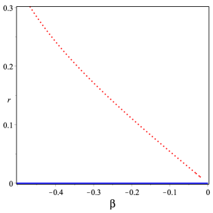
(a)  Spherically symmetric space-time

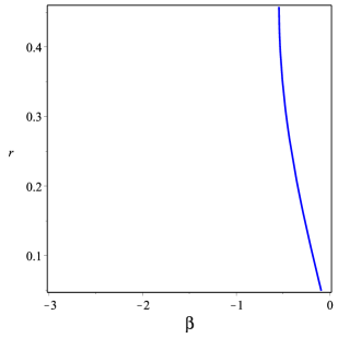
(b)  Spherically symmetric AdS/dS space-time

Figure 8: Plot of the radial coordinate $r$ versus $\beta$ for the black holes in the Einstein frame.

The Hawking temperature for each of these black holes (VI) is given by a lengthy expression, but their behaviors can be easily plotted, see Fig. 9.

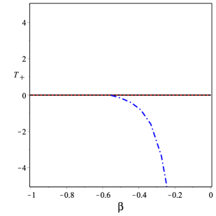
(a)  The black hole solution’s temperature in Einstein’s frame

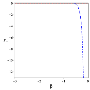
(b)  The black hole solution’s temperature in Einstein’s frame

Figure 9: Plot of the black hole’s temperature versus $\beta$ for the black holes in the Einstein frame.

As is clear from Fig. 9, one gets a negative temperature for both black holes in Einstein’s frame. If we compare the results of the temperatures in the Jordan and Einstein frames we conclude that the physics of the two frames are not equivalent. This investigation shows in a clear way that in spite of the equivalence of the two frames from a mathematical viewpoint, and their sharing of many physical properties, the black hole thermodynamics are not equivalent. The entropy of the black hole (VI) in the Einstein frame is defined as

$${S_{+}} = \pi\bar{r}_{+}{}^{2}.$$ (42)

Using Eq. (42) we compute the entropy of the solutions (VI) as

$${S_{+}}=\frac{\pi}{54\beta^{2}(2\sqrt{36\beta^{2}{\mathcal{K}}^{2}+324\beta^{4}{\mathcal{K}}^{4}-3}-2-36\beta^{2}{\mathcal{K}}^{2})^{3/2}}\Big{[}-4+\sqrt{2\sqrt{36\beta^{2}{\mathcal{K}}^{2}+324\beta^{4}{\mathcal{K}}^{4}-3}-2-36\beta^{2}{\mathcal{K}}^{2}}\Big{(}1+18\beta^{2}{\mathcal{K}}^{2}$$

$$+\sqrt{36\beta^{2}{\mathcal{K}}^{2}+324\beta^{4}{\mathcal{K}}^{4}-3}\Big{)}\Big{]}^{2},$$

$${S_{+}}_{{}_{{}_{{}_{{}_{AdS/dS}}}}}=\pi\bar{r}_{+}{}^{2}.$$ (43)

Eqs. (VII.1) are plotted in Fig. 10, showing that we have a positive entropy. We note that $S$ is proportional to $A$, because of the fact that we are in Einstein’s frame.

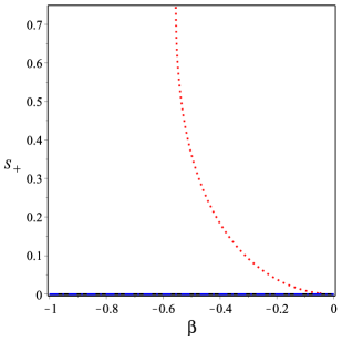
(a)  The entropy of solution (VI)

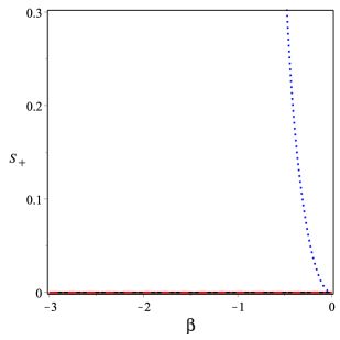
(b)  The entropy of the AdS/dS solution (VI)

Figure 10: Plot of entropy versus $\beta$ for the black holes in the Einstein frame.

Using Eq. (34), the quasi-local energies give

$${E_{+}}_{{}_{{}_{{}_{{}_{\tiny Eq.(\ref{sol})}}}}} = -\frac{1+9\beta^{2}{\mathcal{K}}^{2}-\sqrt{1-18\beta^{2}{\mathcal{K}}^{2}}}{12\beta},$$

$${E_{+}}_{{}_{{}_{{}_{{}_{\tiny Eq.(\ref{sol1})}}}}} = \frac{\bar{r}_{+}}{8}\left(4+3\beta\bar{r}_{+}\right).$$ (44)

The behavior of the quasi local energy is plotted in Fig. 11, which shows that we obtain a positive quasi local energy.

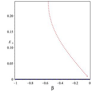
(a)  Black hole solution’s Quasilocal energy

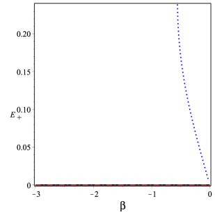
(b)  Black hole solution’s Quasilocal energy

Figure 11: Plot of the quasilocal energies versus $\beta$ for the black holes in Einstein frame.

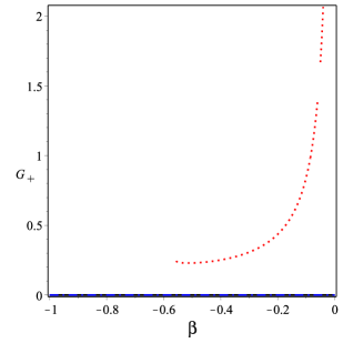
(a)  Black hole solution’s free energy

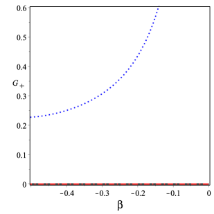
(b)  Black hole solution’s free energy

Figure 12: Plot of the free energy versus $\beta$ for solutions (VI).

Equation (VII.1) shows that $\beta\neq 0$.

The free energy is given by

$$G(r_{+})=E({\bar{r}}_{+})-T({\bar{r}}_{+})S(r{\bar{r}}_{+}).$$ (45)

Using Eqs. (VII.1) and (VII.1) in (45), we get

$${G_{+}}_{{}_{{}_{{}_{{}_{\tiny Eq.(\ref{sol})}}}}}=\frac{(5+9\beta^{2}{\mathcal{K}}^{2})\sqrt{1-18\beta^{2}{\mathcal{K}}^{2}}-5+9\beta^{2}{\mathcal{K}}^{2}}{36\beta(1-\sqrt{1-18\beta^{2}{\mathcal{K}}^{2}})},$$

$${G_{+}}_{{}_{{}_{{}_{{}_{\tiny Eq.(\ref{sol1})}}}}}=\frac{{\bar{r}}_{+}(4+3\beta{\bar{r}}_{+})}{8}+\frac{({\bar{r}}_{+}+2\beta[2\Lambda\alpha{\bar{r}}_{+}{}^{4}+3\beta{\mathcal{K}}^{2}])(1+\beta{\bar{r}}_{+})}{12\beta{\bar{r}}_{+}}.$$ (46)

The behavior of the functions in (VII.1) is depicted in Figs. 1211(a), 1211(b) for particular values of the parameters of the model.

VIII Stability analysis of the black holes in the Jordan and Einstein frames

To study the stability of the black holes we rewrite rewrite Eq. (2) as

$${\mathcal{S}}=\frac{1}{2\kappa}\int d^{4}x\sqrt{-g}\,[\psi\,{\mathcal{R}}-V(\psi)]\,,$$ (47)

where we neglect $\Lambda$. Here the scalar field $\psi$ is coupled to the Ricci scalar and $V(\psi)$ is the potential field Capozziello and De Laurentis (2011). Discussion of the stability of the solutions derived in the previous sections is done through the study of perturbations of spherically symmetric vacuum background spacetime, endowed with the metric

$${\mathrm{d}s^{2}}=g_{\mu\nu}^{BG}dx^{\mu}dx^{\nu}=-w(r)\,dt^{2}+\frac{dr^{2}}{w_{1}(r)}+r^{2}(d\theta^{2}+\sin^{2}\theta\,d\phi^{2}),$$ (48)

$g_{\mu\nu}^{BG}$ being the background metric. We investigate the stability of the black holes obtained in the Jordan and Einstein frames proceeds by using linear perturbations. We have

$$V=-{\frac{4w_{1}\,\psi^{\prime}}{r}}-{\frac{2\psi\,w^{\prime}w_{1}}{wr}}-\frac{\psi^{\prime}w^{\prime}w_{1}}{w}+{\frac{2\psi}{{r}^{2}}}-{\frac{2w_{1}\,\psi}{{r}^{2}}}\,,\qquad\psi^{\prime\prime}=-\frac{w^{\prime}_{1}\psi^{\prime}}{2w_{1}}-\frac{\psi w^{\prime}_{1}}{rw_{1}}+\frac{w^{\prime}\psi^{\prime}}{2w}+\frac{\psi w^{\prime}}{rw}\,,\qquad{\mathcal{R}}=\frac{dV}{d\psi}\,,\\$$ (49)

as background equation of motion in which ^′ stands for differentiation w.r.t $r$.

VIII.1 Brief review of the Regge-Wheeler-Zerilli prescription

We shall now give an outline prescription of the Regge, Wheeler Regge and Wheeler (1957), and Zerilli Zerilli (1970), which can also be used in modified $f({\mathcal{R}})$ gravity Nashed and Capozziello (2019). We start from the slightly perturbed metric corresponding to a static spherically symmetric space-time, $g_{\mu\nu}=g_{\mu\nu}^{BG}+h_{\mu\nu}$, where $h_{\mu\nu}$ stands for an infinitesimal quantity. A scalar field $\Psi(t,r,\theta,\phi)$ can be decomposed as

$$\Psi(t,r,\theta,\phi)=\sum_{\ell,m}\Phi_{\ell m}(t,r)Y_{\ell m}(\theta,\varphi),$$ (50)

where $Y_{\ell m}(\theta,\phi)$ are spherical harmonics. In the same way, one can decompose any vector $V_{a}$ into a divergent and a non-divergent parts, i.e.,

$$V_{a}(t,r,\theta,\phi)=\nabla_{a}\Psi_{1}+E_{a}^{b}\nabla_{b}\Psi_{2},$$ (51)

with $\Psi_{1}$ and $\Psi_{2}$ being two scalars and $E_{ab}\equiv\sqrt{\det\gamma}\leavevmode\nobreak\ \epsilon_{ab}$, where $\gamma_{ab}$ is a 2-dimension metric and $\epsilon_{ab}$ the usual anti-symmetric tensor, where $\epsilon_{\theta\varphi}=1$. The symbol $\nabla_{a}$ stands for the covariant differentiation w.r.t. $\gamma_{ab}$. Eq. (51) shows for the two-component vector $V_{a}$, it is possible to specify it by the two scalar quantities $\Psi_{1}$ and $\Psi_{2}$. Therefore, one can use Eq. (50) with $\Psi_{1}$ and $\Psi_{2}$ in order to express the vector quantity $V_{a}$ in spherical harmonics.

On the other hand, any symmetric tensor $T_{ab}$ can be rewritten as

$$T_{ab}(t,r,\theta,\phi)=\nabla_{a}\nabla_{b}\Psi_{1}+\gamma_{ab}\Psi_{2}+\frac{1}{2}\left(E_{a}{}^{c}\nabla_{c}\nabla_{b}\Psi_{3}+E_{b}{}^{c}\nabla_{c}\nabla_{a}\Psi_{3}\right),$$ (52)

where $\Psi_{1},\leavevmode\nobreak\ \Psi_{2}$ and $\Psi_{3}$ are three scalar quantities since $T_{ab}$ has three independent components. Therefore, one can use the scalar decomposition (50) with $\Psi_{1},\leavevmode\nobreak\ \Psi_{2}$ and $\Psi_{3}$, to determine the tensor $T_{ab}$. The variables corresponding to $E_{ab}$ are the odd-type ones while the rest represent the ones of even-type. The quantities $h_{\mu\nu}$ in the linearized form make odd and even perturbations to fully decouple which makes the above procedure useful to use. In the following subsection we are going to study the perturbations of odd-type.

VIII.2 Perturbative form of $f({\mathcal{R}})$ theory

The odd-types perturbations

From the Regge-Wheeler method, the metric perturbations of odd-type take the form Regge and Wheeler (1957); Zerilli (1970)

$$h_{tt}=0,\leavevmode\nobreak\ \leavevmode\nobreak\ \leavevmode\nobreak\ h_{tr}=0,\leavevmode\nobreak\ \leavevmode\nobreak\ \leavevmode\nobreak\ h_{rr}=0,$$ (53)

$$h_{ta}=\sum_{\ell,m}h_{0,\ell m}(t,r)E_{ab}\partial^{b}Y_{\ell m}(\theta,\varphi),$$ (54)

$$h_{ra}=\sum_{\ell,m}h_{1,\ell m}(t,r)E_{ab}\partial^{b}Y_{\ell m}(\theta,\varphi),$$ (55)

$$h_{ab}=\frac{1}{2}\sum_{\ell,m}h_{2,\ell m}(t,r)\left[E_{a}^{\leavevmode\nobreak\ c}\nabla_{c}\nabla_{b}Y_{\ell m}(\theta,\varphi)+E_{b}^{\leavevmode\nobreak\ c}\nabla_{c}\nabla_{a}Y_{\ell m}(\theta,\varphi)\right].$$ (56)

Using the gauge transformation $x^{\mu}\to x^{\mu}+\xi^{\mu}$, where the components $\xi^{\mu}$ are infinitesimal, one can prove that some components of the metric perturbations are not physical and can be put equal to zero. Now we consider, for the odd perturbations, the following transformation

$$\xi_{t}=\xi_{r}=0,\qquad\qquad\xi_{a}=\sum_{\ell m}\Lambda_{\ell m}(t,r)E_{a}^{\leavevmode\nobreak\ b}\nabla_{b}Y_{\ell m},$$ (57)

where $\Lambda_{\ell m}$ can always be set to vanish. Through this method one can show that $\Lambda_{\ell m}$ is fully fixed which means that they are free from any gauge degrees of freedom. Using Eq. (56) in Eq. (47) and integrating by parts Eq. (47) becomes

$$S_{{odd}}=\frac{1}{2\kappa}\sum_{\ell,m}\int dt\,dr\,{\mathcal{L}}_{{odd}}=\frac{1}{4\kappa}\sum_{\ell,m}\int dt\,dr\,j^{2}\Bigg{[}\frac{\phi\sqrt{w_{1}}}{\sqrt{w}}\Big{\{}{\left({\dot{h}_{1}}-h_{0}^{\prime}\right)}^{2}+\frac{8h_{0}{\dot{h}_{1}}}{r}\Big{\}}+\frac{h_{0}^{2}}{r^{2}}\left\{4r\Bigg{[}\frac{\phi\sqrt{w_{1}}}{\sqrt{w}}\Bigg{]}^{\prime}+4\frac{\phi\sqrt{w_{1}}}{\sqrt{w}}+\frac{(j^{2}-2)\phi}{\sqrt{ww_{1}}}\right\}$$

$$-\frac{\,(j^{2}-2)\,\sqrt{ww_{1}}\,\phi\,h_{1}^{2}}{r^{2}}\Bigg{]},$$ (58)

where we have dropped the suffix $\ell$ for the fields, and $j^{2}=\ell\,(\ell+1)$. Variation of (58) w.r.t. $h_{0}$ yields

$$\Bigg{[}\phi\sqrt{\frac{w_{1}}{w}}(h_{0}^{\prime}-\dot{h}_{1})\Bigg{]}^{\prime}=\frac{h_{0}}{r^{2}}\left\{4r\Bigg{[}\frac{\phi\sqrt{w_{1}}}{\sqrt{w}}\Bigg{]}^{\prime}+4\frac{\phi\sqrt{w_{1}}}{\sqrt{w}}+\frac{(j^{2}-2)\phi}{\sqrt{ww_{1}}}\right\}+\frac{4\phi\sqrt{\frac{w_{1}}{w}}\,\dot{h}_{1}}{r}\,,$$ (59)

that cannot be solved for $h_{0}$. Therefore, we are going to rewrite the action (58) as

$${L}_{{odd}}=\frac{j^{2}\,\phi\sqrt{w_{1}}}{2\sqrt{w}}{\left({\dot{h}_{1}}-h_{0}^{\prime}+\frac{2\,{h_{0}}}{r}\right)}^{2}-\frac{j^{2}\Bigg{(}\frac{\phi\sqrt{w_{1}}}{\sqrt{w}}+r\Bigg{\{}\frac{\phi\sqrt{w_{1}}}{\sqrt{w}}\Bigg{\}}^{\prime}\Bigg{)}\,h_{0}{}^{2}}{r^{2}}+\frac{j^{2}\,h_{0}^{2}}{r^{2}}\left\{4r\Bigg{[}\frac{\phi\sqrt{w_{1}}}{\sqrt{w}}\Bigg{]}^{\prime}+4\frac{\phi\sqrt{w_{1}}}{\sqrt{w}}+\frac{(j^{2}-2)\phi}{\sqrt{ww_{1}}}\right\}-\frac{j^{2}\,(j^{2}-2)\,\sqrt{ww_{1}}\,\phi\,h_{1}^{2}}{r^{2}}.$$ (60)

In Eq. (60) all expressions involving $\dot{h}_{1}$ are collected in first term. Using the Lagrange multiplier, Eq. (60) becomes

$${L}_{{odd}}=\frac{j^{2}\,\psi\sqrt{w_{1}}}{2\sqrt{w}}\left[2\,Q\left(\dot{h}_{{1}}-h^{\prime}_{{0}}+{\frac{2\,h_{{0}}}{r}}\right)-Q^{2}\right]-\frac{j^{2}\Bigg{(}\frac{\psi\sqrt{w_{1}}}{\sqrt{w}}+r\Bigg{\{}\frac{\psi\sqrt{w_{1}}}{\sqrt{w}}\Bigg{\}}^{\prime}\Bigg{)}\,h_{0}{}^{2}}{r^{2}}+\frac{j^{2}\,h_{0}^{2}}{r^{2}}\left\{4r\Bigg{[}\frac{\psi\sqrt{w_{1}}}{\sqrt{w}}\Bigg{]}^{\prime}+4\frac{\psi\sqrt{w_{1}}}{\sqrt{w}}+\frac{j^{2}(j^{2}-2)\phi}{\sqrt{ww_{1}}}\right\}$$

$$-\frac{j^{2}\,(j^{2}-2)\,\sqrt{ww_{1}}\,\phi\,h_{1}^{2}}{r^{2}}.$$ (61)

Eq. (61) shows that the fields, $h_{0}$ and $h_{1}$, take the form

$$h_{1} = -\frac{r^{2}\,\dot{Q}}{(j^{2}-2)w}\,,$$ (62)

$$h_{0} = \frac{r\Bigg{[}\Bigg{(}\frac{2\phi\sqrt{w_{1}}}{\sqrt{w}}+r\Bigg{\{}\frac{\psi\sqrt{w_{1}}}{\sqrt{w}}\Bigg{\}}^{\prime}\Bigg{)}\,Q+\frac{r\,\psi\sqrt{w_{1}}}{2\sqrt{w}}Q^{\prime}\Bigg{]}}{2\Bigg{(}\frac{\psi\sqrt{w_{1}}}{\sqrt{w}}+r\Bigg{\{}\frac{\psi\sqrt{w_{1}}}{\sqrt{w}}\Bigg{\}}^{\prime}\Bigg{)}-\Bigg{(}\frac{\psi\sqrt{w_{1}}}{\sqrt{w}}+r\Bigg{\{}\frac{\psi\sqrt{w_{1}}}{\sqrt{w}}\Bigg{\}}^{\prime}\Bigg{)}}\>.$$ (63)

Eqs. (62) and (63) relate $h_{0}$ and $h_{1}$ to the auxiliary field $Q$. When we know $Q$ the physical modes $h_{0}$ and $h_{1}$ become known. Substituting Eqs. (62) and (63) into Eq. (61) and after some manipulation we get

$${L}_{{odd}}=\frac{s_{1}{}^{2}}{s_{2}}\,\dot{Q}^{2}-\frac{s_{1}{}^{2}\,r^{2}}{s_{3}r^{2}-2rs^{\prime}_{1}-2s_{1}}\,Q^{\prime 2}-\nu_{1}{}^{2}\,Q^{2}\,,$$ (64)

where

$$s_{1}=\frac{j^{2}\psi\sqrt{w_{1}}}{2\sqrt{w}},\qquad s_{2}=\frac{j^{2}\psi(j^{2}-2)\sqrt{ww_{1}}}{2r^{2}},\qquad s_{3}=\frac{j^{2}}{r^{2}}\Bigg{(}\frac{\psi\sqrt{w_{1}}}{\sqrt{w}}+r\Bigg{\{}\frac{\psi\sqrt{w_{1}}}{\sqrt{w}}\Bigg{\}}^{\prime}+\frac{(j^{2}-2)\psi}{2\sqrt{ww_{1}}}\Bigg{)},$$

$$\nu_{1}{}^{2}=\frac{s_{1}r^{2}\Big{[}r^{2}s^{\prime}_{1}s^{\prime}_{3}-r^{2}s^{\prime\prime}_{1}s_{3}+2s_{1}s_{3}+4s^{\prime}_{1}{}^{2}+r^{2}s_{3}{}^{2}-2s_{1}s^{\prime\prime}_{1}+2rs_{1}s^{\prime}_{3}-4rs^{\prime}_{1}s_{3}\Big{]}}{(2s_{1}+2rs^{\prime}_{1}-r^{2}s_{3})^{2}}\,.$$ (65)

Using Eq. (64), one obtains

$$s_{2}\geq 2\,,\qquad{\mbox{that\, leads\, to}\,\,\qquad}j^{2}\geq 2\,,$$

which is the no ghost conditions. One can derive the radial dispersion relation as

$$\omega^{2}=ww_{1}\,k^{2}\,.$$

In the above equation we have assumed that the solutions proportional to $e^{i(\omega t-kr)}$ where $k$ and $\omega$ are large. For the radial speed we get

$$c_{{odd}}^{2}=\left(\frac{dr_{*}}{d\tau}\right)^{2}=1\,,$$

where the radial tortoise coordinate ($dr_{*}^{2}=dr^{2}/w_{1}$) and the proper time ($d\tau^{2}=w_{1}\,dt^{2}$) have been employed.

IX Black hole stability analysis using geodesic deviations in Jordan’s frame

The paths of a test particle in the gravitational field are described by

$${d^{2}x^{\sigma}\over d\tau^{2}}+\left\{{}^{\sigma}_{\mu\nu}\right\}{dx^{\mu}\over d\tau}{dx^{\nu}\over d\tau}=0,$$ (66)

which is known as the geodesic equations. In Eq. (66) $\tau$ represents the affine connection parameter. The geodesic deviation has the form D’Inverno (1992); Nashed (2003)

$${d^{2}\xi^{\sigma}\over d\tau^{2}}+2\left\{{}^{\sigma}_{\mu\nu}\right\}{dx^{\mu}\over d\tau}{d\xi^{\nu}\over d\tau}+\left\{{}^{\sigma}_{\mu\nu}\right\}_{,\ \rho}{dx^{\mu}\over d\tau}{dx^{\nu}\over d\tau}\xi^{\rho}=0,$$ (67)

where $\xi^{\rho}$ is the 4-vector deviation. Introducing (66) and (67) into (9), one can get

$${d^{2}t\over d\tau^{2}}=0,\qquad{1\over 2}w^{\prime}(r)\left({dt\over d\tau}\right)^{2}-r\left({d\phi\over d\tau}\right)^{2}=0,\qquad{d^{2}\theta\over d\tau^{2}}=0,\qquad{d^{2}\phi\over d\tau^{2}}=0,$$ (68)

and for the geodesic deviation

$${d^{2}\xi^{1}\over d\tau^{2}}+w(r)w^{\prime}(r){dt\over d\tau}{d\xi^{0}\over d\tau}-2rw(r){d\phi\over d\tau}{d\xi^{3}\over d\tau}+\left[{1\over 2}\left(w^{\prime 2}(r)+w(r)w^{\prime\prime}(r)\right)\left({dt\over d\tau}\right)^{2}-\left(w(r)+rw^{\prime}(r)\right)\left({d\phi\over d\tau}\right)^{2}\right]\xi^{1}=0,$$

$${d^{2}\xi^{0}\over d\tau^{2}}+{w^{\prime}(r)\over w(r)}{dt\over d\tau}{d\zeta^{1}\over d\tau}=0,\qquad{d^{2}\xi^{2}\over d\tau^{2}}+\left({d\phi\over d\tau}\right)^{2}\xi^{2}=0,\qquad\qquad{d^{2}\xi^{3}\over d\tau^{2}}+{2\over r}{d\phi\over d\tau}{d\xi^{1}\over d\tau}=0,$$ (69)

where $w(r)$ is defined by the metric (18) or (19), $w^{\prime}(r)=\displaystyle{dw(r)\over dr}$. Using the circular orbit

$$\theta={\pi\over 2},\qquad{d\theta\over d\tau}=0,\qquad{dr\over d\tau}=0,$$ (70)

we get

$$\left({d\phi\over d\tau}\right)^{2}={w^{\prime}(r)\over r[2w(r)-rw^{\prime}(r)]},\qquad\left({dt\over d\tau}\right)^{2}={2\over 2w(r)-rw^{\prime}(r)}.$$ (71)

Eqs. (IX) can be rewritten as

$${d^{2}\xi^{1}\over d\phi^{2}}+w(r)w^{\prime}(r){dt\over d\phi}{d\xi^{0}\over d\phi}-2rw(r){d\xi^{3}\over d\phi}+\left[{1\over 2}\left[w^{\prime 2}(r)+w(r)w^{\prime\prime}(r)\right]\left({dt\over d\phi}\right)^{2}-\left[w(r)+rw^{\prime}(r)\right]\right]\zeta^{1}=0,$$

$${d^{2}\xi^{2}\over d\phi^{2}}+\xi^{2}=0,\qquad{d^{2}\xi^{0}\over d\phi^{2}}+{w^{\prime}(r)\over w(r)}{dt\over d\phi}{d\xi^{1}\over d\phi}=0,\qquad{d^{2}\xi^{3}\over d\phi^{2}}+{2\over r}{d\xi^{1}\over d\phi}=0.$$ (72)

The second equation of (IX) corresponds to a simple harmonic motion, which means that there is stability on the plane $\theta=\pi/2$. Assuming the remaining equations of (IX) have solutions of the form

$$\xi^{0}=\zeta_{1}e^{i\sigma\phi},\qquad\xi^{1}=\zeta_{2}e^{i\sigma\phi},\qquad and\qquad\xi^{3}=\zeta_{3}e^{i\sigma\phi},$$ (73)

where $\zeta_{1},\zeta_{2}$ and $\zeta_{3}$ are constant and $\phi$ is an unknown variable. Using Eq. (73) into (IX), one can get the stability condition for a static spherically symmetric charged black hole in the form

$$\frac{3ww^{\prime}-\sigma^{2}w^{\prime}-2rw^{\prime 2}+rww^{\prime\prime}}{w^{\prime}}>0.$$ (74)

Eq. (74) for solutions (18) and (19) becomes

$$\sigma^{2}=\frac{2r^{2}+\beta r^{3}+18{\mathcal{K}}^{2}\beta r+48\beta^{2}{\mathcal{K}}^{4}+4r^{4}\beta\Lambda[5r+4r^{2}\beta+24\beta{\mathcal{K}}^{2}]}{2\beta r^{2}(r+6\beta{\mathcal{K}}^{2}+4r^{4}\beta\Lambda)}>0.$$ (75)

Fig. 13 is a plot of Eq. (75) for particular values of the models. It exhibits the regions where the black holes are stable and the regions where there is no possible stability.

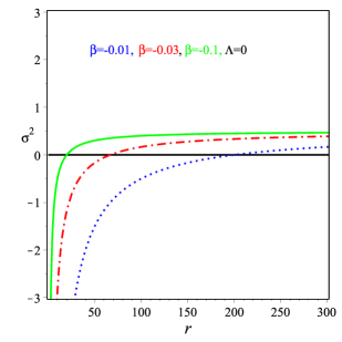
(a)  Stability of (75) when $\Lambda=0$

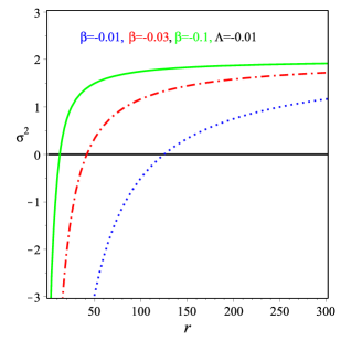
(b)  Stability of (75) when $\Lambda\neq 0$

Figure 13: Schematic plot of Eq. (75), namely $\sigma^{2}$ versus the coordinate $r$.

IX.1 Black hole stability analysis using geodesic deviation in Einstein’s frame

Introducing (66) and (67) into (VI), we get for the geodesic equations

$${d^{2}t\over d\tau^{2}}=0,\qquad{1\over 2}w^{\prime}_{1}(\bar{r})\left({dt\over d\tau}\right)^{2}-\bar{r}\left({d\phi\over d\tau}\right)^{2}=0,\qquad{d^{2}\theta\over d\tau^{2}}=0,\qquad{d^{2}\phi\over d\tau^{2}}=0,$$ (76)

and for the geodesic deviation we have

$${d^{2}\xi^{1}\over d\tau^{2}}+w(\bar{r})w^{\prime}_{1}(\bar{r}){dt\over d\tau}{d\xi^{0}\over d\tau}-2\bar{r}w(\bar{r}){d\phi\over d\tau}{d\xi^{3}\over d\tau}+\left[{1\over 2}\left[w^{\prime}(\bar{r})w^{\prime}_{1}(\bar{r})+w(\bar{r})w^{\prime\prime}_{1}(\bar{r})\right]\left({dt\over d\tau}\right)^{2}-\left[w(\bar{r})+\bar{r}w^{\prime}(\bar{r})\right]\left({d\phi\over d\tau}\right)^{2}\right]\xi^{1}=0,$$

$${d^{2}\xi^{0}\over d\tau^{2}}+{w^{\prime}_{1}(\bar{r})\over w_{1}(\bar{r})}{dt\over d\tau}{d\zeta^{1}\over d\tau}=0,\qquad{d^{2}\xi^{2}\over d\tau^{2}}+\left({d\phi\over d\tau}\right)^{2}\xi^{2}=0,\qquad\qquad{d^{2}\xi^{3}\over d\tau^{2}}+{2\over\bar{r}}{d\phi\over d\tau}{d\xi^{1}\over d\tau}=0,$$ (77)

where $w(\bar{r})$ is defined by the metric (VI) $w^{\prime}(\bar{r})=\displaystyle{dw(\bar{r})\over d\bar{r}}$ and $w^{\prime}_{1}(\bar{r})=\displaystyle{dw_{1}(\bar{r})\over d\bar{r}}$. Using the circular orbit

$$\theta={\pi\over 2},\qquad{d\theta\over d\tau}=0,\qquad{d\bar{r}\over d\tau}=0,$$ (78)

we get

$$\left({d\phi\over d\tau}\right)^{2}={w^{\prime}_{1}(\bar{r})\over\bar{r}[2w(\bar{r})-\bar{r}w^{\prime}(\bar{r})]},\qquad\left({dt\over d\tau}\right)^{2}={2\over 2w(\bar{r})-w^{\prime}(\bar{r})}.$$ (79)

Eqs. (IX.1) can be rewritten as

$${d^{2}\xi^{1}\over d\phi^{2}}+w(\bar{r})w^{\prime}_{1}(\bar{r}){dt\over d\phi}{d\xi^{0}\over d\phi}-2\bar{r}w^{\prime}(\bar{r}){d\xi^{3}\over d\phi}+\left[{1\over 2}\left[w^{\prime}(\bar{r})w^{\prime}_{1}(\bar{r})+w(\bar{r})w^{\prime\prime}_{1}(\bar{r})\right]\left({dt\over d\phi}\right)^{2}-\left[w(\bar{r})+\bar{r}w^{\prime}(\bar{r})\right]\right]\zeta^{1}=0,$$

$${d^{2}\xi^{2}\over d\phi^{2}}+\xi^{2}=0,\qquad{d^{2}\xi^{0}\over d\phi^{2}}+{w^{\prime}(\bar{r})\over w(\bar{r})}{dt\over d\phi}{d\xi^{1}\over d\phi}=0,\qquad{d^{2}\xi^{3}\over d\phi^{2}}+{2\over\bar{r}}{d\xi^{1}\over d\phi}=0.$$ (80)

Eqs. (IX.1) corresponds to simple harmonic motion what means we have a stability at the plane $\theta=\pi/2$. The remanning equations of (IX.1) admit the following solutions

$$\xi^{0}=\zeta_{1}e^{i\omega\phi},\qquad\xi^{1}=\zeta_{2}e^{i\omega\phi},\qquad and\qquad\xi^{3}=\zeta_{3}e^{i\omega\phi},$$ (81)

where $\zeta_{1},\zeta_{2}$ and $\zeta_{3}$ are constants and $\phi$ is unknown. Using Eq. (81) into (IX.1) one gets a quite lengthy expression, which is depicted in Fig. 14. This plot shows that black holes in the Einstein frame have always some non-void stability region.

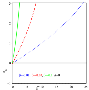
(a)  Stability of (IX.1) when $\Lambda=0$

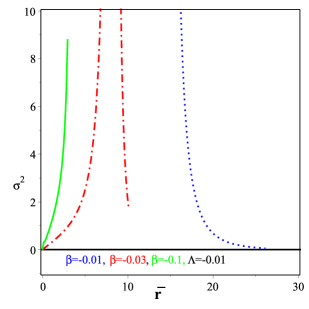
(b)  Stability of (IX.1) when $\Lambda\neq 0$

Figure 14: Schematic plot of Eq. (IX.1), namely $\sigma^{2}$ versus the coordinate $r$.

IX.2 Causal structure of the solutions

We shall now discuss the causal structure of the space-time (13). For this purpose, we start from the metric

$$ds^{2}=-\mathrm{e}^{2\nu(r)}dt^{2}+\mathrm{e}^{-2\nu(r)}dr^{2}+r^{2}\sum_{i,j=1}^{2}\tilde{g}_{ij}dx^{i}dx^{j}\,,$$ (82)

with

$$\mathrm{e}^{2\nu}=C^{2}-\frac{M}{r}\,,\quad C>0\,,$$ (83)

the metric of the unit sphere being $\tilde{g}_{ij}$, and we consider the region where $r\gg M$. Then, the metric in (82) reduces to

$$ds_{\mathrm{as}}^{2}=-C^{2}dt^{2}+\frac{dr^{2}}{C^{2}}+r^{2}\sum_{i,j=1}^{2}\tilde{g}_{ij}dx^{i}dx^{j}\,.$$ (84)

Redefining,

$$t=\frac{\tilde{t}}{C}\,,\quad r=C\tilde{r}\,,$$ (85)

we find

$$ds_{\mathrm{as}}^{2}=-d{\tilde{t}}^{2}+d{\tilde{r}}^{2}+C^{2}{\tilde{r}}^{2}\sum_{i,j=1}^{2}\tilde{g}_{ij}dx^{i}dx^{j}\,,$$ (86)

which is not Lorentz invariant unless $C=1$. In order to clarify the situation, we choose $\tilde{g}_{ij}$ as

$$\sum_{i,j=1}^{2}\tilde{g}_{ij}dx^{i}dx^{j}=d\theta^{2}+\sin^{2}\theta d\phi^{2}\,,$$ (87)

with $0\leq\theta\leq\pi$ and $0\leq\phi<2\pi$, and we consider the hypersurface with $\theta=\frac{\pi}{2}$. Then, the metric reads

$$ds_{\mathrm{hyp}}^{2}=-d{\tilde{t}}^{2}+d{\tilde{r}}^{2}+C^{2}d\phi^{2}\,.$$ (88)

If we redefine,

$$\phi=C^{-1}\tilde{\phi}\,,$$ (89)

the metric acquires the following form

$$ds_{\mathrm{hyp}}^{2}=-d{\tilde{t}}^{2}+d{\tilde{r}}^{2}+d{\tilde{\phi}}^{2}\,,$$ (90)

which is nothing but the metric of flat three-dimensional space-time. We should note, however, that $0\leq\tilde{\phi}\leq 2C\pi$, and therefore if $C<1$, a deficit angle appears, while if $C>1$ a surplus angle shows up (see Fig. 15 for the case $C=\frac{3}{4}<1$ and Fig. 16 for the case $C=\frac{5}{4}>1$). For $C<1$ the light emitted from a point reaches another point in two orbits of the light trajectory (see Fig. 17) and, therefore, multiple light-cone surfaces are formed. On the contrary, in the other case the light ray emitted from a point $\tilde{\phi}=\pi$ and $\tilde{r}=r_{0}$ ($r_{0}$ is a constant) does not reach the region $2\pi<\tilde{\phi}<2C\pi$ (see Fig. 18) and, therefore, the light-cone surface has a boundary. In such space-time, one cannot separate time-like regions from space-like ones and all kind of problems with causality may show up.

Figure 15: Structure of the spatial part for $C=\frac{3}{4}<1$. We identify two arrows and glue the space there.

Figure 16: Structure of the spatial part for $C=\frac{5}{4}>1$. We identify two arrow and glue the space there.

Figure 17: The point $B^{\prime}$ is identified with the point $B$. When $C=\frac{3}{4}<1$, the light emitted at point $A$ may reach point $B=B^{\prime}$ along two different paths.

Figure 18: When $C=\frac{5}{4}>1$, the light emitted at point $A$ ($\tilde{\phi}=\pi$ and $\tilde{r}=r_{0}$, $r_{0}$ is a constant) cannot reach the shaded region ($2\pi<\tilde{\phi}<\frac{5}{2}\pi=2C\pi$).

X Alternative black hole description from a generalized fluid model

X.1 Relation between the space-time geometry and an equation of state

We will here consider the relation existing between the space-time geometry and an equation of state for General Relativity with a cosmological fluid. We start from the space-time metric (82), from where we have

$$R_{tt}= \frac{1}{2}\left(C+\frac{r^{2}}{l^{2}}-\frac{M}{r}+\frac{q^{2}}{r^{2}}\right)\left(\frac{6}{l^{2}}+\frac{2q^{2}}{r^{4}}\right)\,,$$

$$R_{rr}= -\frac{1}{2}\left(C+\frac{r^{2}}{l^{2}}-\frac{M}{r}+\frac{q^{2}}{r^{2}}\right)^{-1}\left(\frac{6}{l^{2}}+\frac{2q^{2}}{r^{4}}\right)\,,$$

$$R_{ij}= \left(1-C-\frac{3r^{2}}{l^{2}}+\frac{q^{2}}{r^{2}}\right)\tilde{g}_{ij}\,,$$

$$R= -\frac{12}{l^{2}}-\frac{2\left(C-1\right)}{r^{2}}\,.$$ (91)

Using now the Einstein equation

$$R_{\mu\nu}-\frac{1}{2}g_{\mu\nu}R=\kappa^{2}T_{\mu\nu}\,,$$ (92)

we find

$$\kappa^{2}T_{tt}= -\kappa^{2}T_{rr}=\left(C+\frac{r^{2}}{l^{2}}-\frac{M}{r}+\frac{q^{2}}{r^{2}}\right)\left(-\frac{3}{l^{2}}-\frac{C-1}{r^{2}}+\frac{q^{2}}{r^{4}}\right)\,,$$

$$\kappa^{2}T_{ij}= \left(\frac{3r^{2}}{l^{2}}+\frac{q^{2}}{r^{2}}\right)\tilde{g}_{ij}$$ (93)

We now define the energy density $\rho$, the pressure in the radial direction $p_{r}$, and the pressure in the angular direction $p_{a}$, as

$$T_{tt}=-g_{tt}\rho\,,\quad T_{rr}=g_{rr}p_{r}\,,\quad T_{ij}=g_{ij}p_{a}\,,$$ (94)

with the result

$$\kappa^{2}\rho=-\left(-\frac{3}{l^{2}}-\frac{C-1}{r^{2}}+\frac{q^{2}}{r^{4}}\right)\,,\quad\kappa^{2}p_{r}=-\left(-\frac{3}{l^{2}}-\frac{C-1}{r^{2}}+\frac{q^{2}}{r^{4}}\right)\,,\quad\kappa^{2}p_{a}=\frac{3}{l^{2}}+\frac{q^{2}}{r^{4}}\,,$$ (95)

which yields the following equation of state (EoS) for the cosmic fluid

$$\rho=p_{r}=-p_{a}+\frac{6}{\kappa^{2}l^{2}}+\frac{C-1}{\kappa^{2}q}\sqrt{\kappa^{2}p_{a}-\frac{3}{l^{2}}}\,.$$ (96)

In particular, when $\frac{1}{l}=0$, we find

$$\rho=p_{r}=-p_{a}+\frac{C-1}{\kappa q}\sqrt{p_{a}}\,.$$ (97)

Eq. (96) tells us that $p_{a}\geq\frac{3}{\kappa^{2}l^{2}}$, and so the quantity inside the square root is positive. In particular, in the case $\frac{1}{l}=0$, as in (97), we find $p_{a}\geq 0$. And, in order that $\rho\geq 0$, we get $p_{a}\leq\frac{\left(C-1\right)^{2}}{\kappa^{2}q^{2}}$. Then, it follows that

$$0\leq p_{a}\leq\frac{\left(C-1\right)^{2}}{\kappa^{2}q^{2}}\,.$$ (98)

In the case $\frac{1}{l}\neq 0$, corresponding to Eq. (96), the restriction associated to (97) becomes somehow involved, as follows

$$\frac{3}{\kappa^{2}l^{2}}\leq p_{a}\leq\frac{1}{2}\left(\frac{12}{\kappa^{2}l^{2}}+\frac{\left(C-1\right)^{2}}{\kappa^{2}q^{2}}+\sqrt{\frac{12\left(C-1\right)^{2}}{\kappa^{4}l^{2}q^{2}}+\frac{\left(C-1\right)^{4}}{\kappa^{4}q^{4}}}\right)\,.$$ (99)

For $\frac{1}{l}=0$ in (97), the pressures $p_{r}$ and $p_{a}$ should be positive if we assume that the energy density $\rho$ is positive. We should note, however, that when $\frac{1}{l^{2}}<0$ in (96), $p_{a}$ can be negative, as indeed found from (100). Therefore, this fluid can act as dark energy, what is indeed clear from the assumption (82), where the metric behaves as the de Sitter space-time for large $r$, when $\frac{1}{l^{2}}<0$.

$$p_{a}^{2}-\frac{12}{\kappa^{2}l^{2}}+\frac{36}{\kappa^{2}l^{2}}p_{a}=\frac{\left(C-1\right)^{2}}{\kappa^{4}q^{2}}\left(\kappa^{2}p_{a}-\frac{3}{l^{2}}\right)$$

$$\frac{3}{\kappa^{2}l^{2}}\leq p_{a}\leq\frac{1}{2}\left(\frac{12}{\kappa^{2}l^{2}}+\frac{\left(C-1\right)^{2}}{\kappa^{2}q^{2}}+\sqrt{\left(\frac{12}{\kappa^{2}l^{2}}+\frac{\left(C-1\right)^{2}}{\kappa^{2}q^{2}}\right)^{2}-\frac{144}{\kappa^{4}l^{4}}-\frac{12\left(C-1\right)^{2}}{\kappa^{4}l^{2}q^{2}}}\right)\,.$$ (100)

In summary, we have here derived the same BH solution as in usual general relativity with a cosmological fluid, which may be intrepreted as kin ad of dark energy. This is a clear indication of the universality of the BH solution under discussion in this paper.

XI Discussion and conclusions

We have obtained, in this paper, a genuinely new type of charged black holes, with electric and magnetic charges, in the context of a particular class of $f(R)$ modified gravity. We have provided a detailed description of their physical properties, including their stability and causal structure, both in the Jordan and in the Einstein frames. Being more specific, we have worked with the following forms for $f(R)$, namely $f(R)=R+2\beta\sqrt{R}$ and $f(R)=R+2\beta\sqrt{R-8\Lambda}$, to produce flat and AdS/dS space-times, respectively, and solved the field equations of $f(R)$ for a spherically symmetric space-time in which $g_{tt}=\frac{1}{g_{rr}}$. We have solved the resulting field equations in an exact way and derived black holes, which are characterized by three parameters: the mass, which depends on the dimensional parameter $\beta$, bound to have a negative value, and the electric and magnetic charges.

The Ricci scalar of the black holes here found is non-trivial. It has the form $R=\frac{1}{r^{2}}$, for the case of flat space-time, and $R=\frac{1}{r^{2}}+8\Lambda$ for the AdS/dS space-times. A most remarkable result is that these black holes cannot be reduced to the ordinary ones appearing in Einstein’s GR; in other words, they are genuinely new black holes of the modified $f(R)$ gravities. We have calculated the scalar invariants of these solutions and shown that $\beta\neq 0$. The calculations involving the scalar fields have shown that one gets a true singularity at $r=0$. Using conformal transformation, we got charged black hole solutions in the realm of the Einstein frame. An interesting feature of the black holes obtained in this frame is the fact that $g_{tt}\neq\frac{1}{g_{rr}}$, what does not happen for the corresponding black holes in the Jordan frame. However, in spite of the fact that the black holes have different $g_{tt}$ and $g^{rr}$ components for the metric in the Einstein frame, they have coinciding Killing and event horizons.

It is well know that the Jordan and the Einstein frames are mathematically equivalent. To check if their corresponding associated physics are equivalent, too, we have calculated some thermodynamical quantities for the above black holes, respectively obtained in one and in the other frame. A detailed discussion has shown that the physics associated with the entropy, quasi-local energy, and Gibbs free energy, in both frames, turn out to be fully equivalent. However, the physics associated to the Hawking temperature is not the same in both frames: the temperature in the Jordan frame is always positive, contrary to what happens in the Einstein frame, which can lead to negative values of yhe same. This may serve as an indication that the physics of the two frames are not equivalent, at least concerning this important quantity, the black hole temperature. An intriguing conjecture that has come to our minds is the following: could this possibly be related to the loss-of-information paradox?

Going more deeply into the black hole properties, we have studied their stability using linear perturbations. Our calculations show that the radial propagation speed always equals one, in both frames, which means that the constructed black holes are stable. In addition, we have used the procedure of geodesic deviation to study the stability of the black holes, both in the Jordan and in the Einstein frames, and derived in each case the stability condition. Finally, we have also studied the causal structure of our novel black holes. We have shown that, in general, they are not invariant under Lorentz transformations. Moreover, we have identified that there is a (positive or negative) deficit angle associated with them. It goes without saying that the black holes obtained in this work need still to be analyzed in more depth, in order to unveil all of their physical properties, a job we hope to undertake elsewhere. Furthermore, an extension of this study to less symmetric backgrounds and to a more general form of $f(R)$ is pending.

We now consider the possibility that the black hole corresponding to the solution (13) can be found by any observation. The analysis in Section IXB tell that the solution (13) corresponds to $C=\frac{1}{\sqrt{2}}$ in (82) with (83). Because $C=\frac{1}{\sqrt{2}}<1$, the solution makes the deficit angle. Then Figure 17 tells that the black hole generates strong gravitational lensing effects. In the usual black hole, the lensing effects occur only in the region near the black hole but for the geometry expressed by the metric (13) the effects occur in a rather large region, say interstellar region, around the black hole. Therefore the big ring much greater than the standard Einstein ring or double images separated in a large angle could be observed as in the observation of the standard weak lensing as in Hildebrandt et al. (2017); Joudaki et al. (2018); Aghanim et al. (2018) in future.

Appendix A

The field equations of Ansatz (9) without cosmological constant

Imposing the Ansatz (9) to Eqs. (4), (5) and (7), after using Eq. (10), we get

$$\zeta_{t}{}^{t}=\frac{1}{4r^{6}\sin^{2}\theta\sqrt{{\mathcal{R}}^{5}}}\Big{\{}4r^{2}\sqrt{{\mathcal{R}}^{5}}\Big{[}r^{2}\sin^{2}\theta(rw^{\prime}+wn_{\theta}{}^{2}-2ws^{\prime}n_{\theta}+q^{\prime 2}r^{2}-1+w\{1+s^{\prime 2}\})+k_{\theta}{}^{2}+r^{2}wp^{\prime 2}\Big{]}+\beta\sin^{2}\theta\Big{[}r^{6}w{\mathcal{R}}w^{\prime\prime\prime\prime}+3r^{6}ww^{\prime\prime\prime 2}\\$$

$$-r^{3}w^{\prime\prime\prime}(r^{2}w^{\prime\prime}[rw^{\prime}-12w]+4r^{2}w^{\prime 2}+2rw^{\prime}[31w-1]-48w[1-w])+2r^{6}w^{\prime\prime 3}-4r^{4}w^{\prime\prime 2}(4-6rw^{\prime}-15w)+2r^{2}w^{\prime\prime}(57r^{2}w^{\prime 2}\\$$

$$+14r[3w-5]w^{\prime}-36w^{2}+20+16w)+200r^{3}w^{\prime 3}+4r^{2}w^{\prime 2}(96w-85)+8rw^{\prime}[w-1][27w-23]+32[w-1]^{2}[2w-1]\Big{]}\Big{\}}=0,$$

$$\zeta_{t}{}^{\theta}=\frac{2q^{\prime}w(n_{\theta}-s^{\prime})}{r^{2}}=0,\qquad\zeta_{t}{}^{\phi}=\frac{2q^{\prime}fp^{\prime}}{r^{2}\sin^{2}\theta}=0,\qquad\zeta_{r}{}^{\theta}=\frac{2p^{\prime}k_{\theta}}{r^{4}\sin^{2}\theta}=0,\qquad\zeta_{r}{}^{\phi}=\frac{2(n_{\theta}-s^{\prime})k_{\theta}}{r^{4}\sin^{2}\theta}=0,$$

$$\zeta_{r}{}^{r}=\frac{1}{4r^{4}\sin^{2}\theta\sqrt{{\mathcal{R}}^{3}}}\Big{\{}4\sqrt{{\mathcal{R}}^{3}}\Big{[}r^{2}\sin^{2}\theta(rw^{\prime}-wn_{\theta}{}^{2}+2ws^{\prime}n_{\theta}-ws^{\prime 2}+[w-1+r^{2}q^{\prime 2}])+k^{\prime 2}-wr^{2}p^{\prime 2}\Big{]}+\beta\sin^{2}\theta\Big{(}r^{2}w^{\prime\prime\prime}[4w+rw^{\prime}]\\$$

$$-2r^{4}w^{\prime\prime 2}+w^{\prime\prime}[4r^{2}(3+w)-16r^{3}w^{\prime}]-50r^{2}w^{\prime 2}+4rw^{\prime}(15-17w)-16(1-3w+2w^{2})\Big{)}\Big{\}}=0,$$

$$\zeta_{\theta}{}^{t}=2q^{\prime}(n_{\theta}-s^{\prime})=0,\qquad\zeta_{\theta}{}^{r}=\frac{2wk_{\theta}p^{\prime}}{r^{2}\sin^{2}\theta},\qquad\zeta_{\theta}{}^{\phi}=\frac{2w(n_{\theta}-s^{\prime})p^{\prime}}{r^{2}\sin^{2}\theta},\qquad\zeta_{\phi}{}^{t}=2q^{\prime}p^{\prime}=0,$$

$$\zeta_{\phi}{}^{r}=\frac{2w(n_{\theta}-s^{\prime})k_{\theta}}{r^{2}}=0,\qquad\zeta_{\phi}{}^{\theta}=\frac{2wp^{\prime}(n_{\theta}-s^{\prime})}{r^{2}}=0,$$

$$\zeta_{\theta}{}^{\theta}=\frac{1}{2r^{6}\sin^{2}\theta\sqrt{{\mathcal{R}}^{5}}}\Big{\{}2r^{2}\sqrt{{\mathcal{R}}^{5}}\Big{[}r^{2}\sin^{2}\theta\Big{(}\frac{r^{2}w^{\prime\prime}}{2}+rw^{\prime}-wn_{\theta}{}^{2}+2wn_{\theta}s^{\prime}-q^{\prime 2}r^{2}-ws^{\prime 2}\Big{)}-k_{\theta}{}^{2}+2l_{\phi}k_{\theta}+r^{2}wp^{\prime 2}\Big{]}-\beta\sin^{2}\theta\Big{[}r^{6}w{\mathcal{R}}w^{\prime\prime\prime\prime}\\$$

$$+\frac{3r^{6}ww^{\prime\prime\prime 2}}{2}-r^{3}w^{\prime\prime\prime}(r^{2}w^{\prime\prime}[rw^{\prime}-7w]+4r^{2}w^{\prime 2}+2rw^{\prime}[14w-1]-22w[1-w])+2r^{6}w^{\prime\prime 3}-2r^{4}w^{\prime\prime 2}\Big{(}5-9rw^{\prime}-18w\Big{)}+2r^{2}w^{\prime\prime}(33r^{2}w^{\prime 2}\\$$

$$+r[27w-34]w^{\prime}-18w^{2}+8+10w)]+104r^{3}w^{\prime 3}+2r^{2}w^{\prime 2}(81w-74)+4rw^{\prime}[15w-16][w-1]-4(2-8w+10w^{2}-4w^{3})\Big{\}}=0,$$

$$\zeta_{\phi}{}^{\phi}=\frac{1}{2r^{6}\sin^{2}\theta\sqrt{{\mathcal{R}}^{5}}}\Big{\{}2r^{2}\sqrt{{\mathcal{R}}^{5}}\Big{[}r^{2}\sin^{2}\theta\Big{(}\frac{r^{2}w^{\prime\prime}}{2}+rw^{\prime}+wn_{\theta}{}^{2}-2wn_{\theta}s^{\prime}-q^{\prime 2}r^{2}+ws^{\prime 2}\Big{)}-k_{\theta}{}^{2}-r^{2}wp^{\prime 2}\Big{]}-\beta\sin^{2}\theta\Big{[}r^{6}w{\mathcal{R}}w^{\prime\prime\prime\prime}\\$$

$$+\frac{3r^{6}ww^{\prime\prime\prime 2}}{2}-r^{3}w^{\prime\prime\prime}(r^{2}w^{\prime\prime}[rw^{\prime}-7w]+4r^{2}w^{\prime 2}+2rw^{\prime}[14w-1]-22w[1-w])+2r^{6}w^{\prime\prime 3}-2r^{4}w^{\prime\prime 2}\Big{(}5-9rw^{\prime}-18w\Big{)}+2r^{2}w^{\prime\prime}(33r^{2}w^{\prime 2}\\$$

$$+r[27w-34]w^{\prime}-18w^{2}+8+10w)]+104r^{3}w^{\prime 3}+2r^{2}w^{\prime 2}(81w-74)+4rw^{\prime}[15w-16][w-1]-4(2-8w+10w^{2}-4w^{3})\Big{\}}=0,$$

$$\zeta=\frac{1}{2r^{6}\sqrt{{\mathcal{R}}^{5}}}\Big{\{}2r^{6}\sqrt{{\mathcal{R}}^{5}}-3\beta\Big{[}r^{6}w{\mathcal{R}}w^{\prime\prime\prime\prime}+\frac{3r^{6}ww^{\prime\prime\prime 2}}{2}-r^{3}w^{\prime\prime\prime}(r^{2}w^{\prime\prime}[rw^{\prime}-6w]+4r^{2}w^{\prime 2}+2rw^{\prime}[31w-1]-24w[1-w])+2r^{6}w^{\prime\prime 3}\\$$

$$-2r^{4}w^{\prime\prime 2}\Big{(}6-10rw^{\prime}-17w\Big{)}+2r^{2}w^{\prime\prime}(41r^{2}w^{\prime 2}+2r[16w-23]w^{\prime}-16w^{2}+12+4w)+136r^{3}w^{\prime 3}+2r^{2}w^{\prime 2}(117w-106)\\$$

$$+8rw^{\prime}[15w-13][w-1]+16(2w-1)(w-1)^{2}\Big{]}\Big{\}}=0,$$

where $q(r)$, $n(\theta)$, $s(r)$, $l(\phi)$, $p(r)$, and $k(\theta)$ are the gauge potentials, defined as

$$\xi:=q(r)dt+n(\theta)dr+s(r)d\theta+[p(r)+k(\theta)]d\phi.$$

For brevity, we put $w^{\prime}=\frac{dw}{dr}$, $w^{\prime\prime}=\frac{d^{2}w}{dr^{2}}$, $w^{\prime\prime\prime}=\frac{d^{3}w}{dr^{3}}$, $w^{\prime\prime\prime\prime}=\frac{d^{4}w}{dr^{4}}$, $q^{\prime}=\frac{dq}{dr}$, $s^{\prime}=\frac{ds}{dr}$, $p^{\prime}=\frac{dm}{dr}$ $n_{\theta}=\frac{dn}{d\theta}$ and $k_{\theta}=\frac{dk}{d\theta}$. We must note that, when the magnetic fields vanish, i.e. $n=s=p=k=0$, we get $\zeta_{\theta}{}^{\theta}=\zeta_{\phi}{}^{\phi}$, and in this case the field equation $({A\cdot 1})$ $\sim$ $({A\cdot 8})$ coincides with the one derived in Nashed and Capozziello (2019).

Appendix B

The field equations of Ansatz (9) with cosmological constant

Now

$$\zeta_{t}{}^{t}=\frac{1}{4r^{9}\sin^{2}\theta\sqrt{{\textrm{R}}^{5}}}\Big{\{}4r^{5}\sqrt{{\textrm{R}}^{5}}\Big{[}r^{2}\sin^{2}\theta(rw^{\prime}+wn_{\theta}{}^{2}-2ws^{\prime}n_{\theta}+q^{\prime 2}r^{2}-1+2r^{2}\Lambda+w\{1+s^{\prime 2}\})+k_{\theta}{}^{2}+r^{2}+wp^{\prime 2}\Big{]}+\beta\sin^{2}\theta\Big{[}r^{6}w{\textrm{R}}w^{\prime\prime\prime\prime}\\$$

$$+3r^{6}ww^{\prime\prime\prime 2}-r^{3}w^{\prime\prime\prime}(r^{2}w^{\prime\prime}[rw^{\prime}-12w]+4r^{2}w^{\prime 2}+2rw^{\prime}[31w-1+4r^{2}\Lambda]+48w[1-w-2r^{2}\Lambda])+2r^{6}w^{\prime\prime 3}-4r^{4}w^{\prime\prime 2}\Big{(}4-6rw^{\prime}-15w\\$$

$$-16r^{2}\Lambda\Big{)}+2r^{2}w^{\prime\prime}(57r^{2}w^{\prime 2}+14r[3w-5+8r^{2}\Lambda]w^{\prime}-36w^{2}+80[4r^{2}\Lambda-1]^{2}+16w[1+9r^{2}\Lambda])+200r^{3}w^{\prime 3}+4r^{2}w^{\prime 2}\Big{(}96w-85\\$$

$$+324r^{2}\Lambda\Big{)}+8rw^{\prime}\Big{\{}27w^{2}-23+2w(47r^{2}\Lambda-50)+11w^{3}+5w^{2}(1-2r^{2}\Lambda)+w(2+24r^{4}\Lambda^{2}-11r^{2}\Lambda)+(4r^{2}\Lambda-1)^{3}\Big{\}}\Big{]}\Big{\}}=0,$$

$$\zeta_{t}{}^{\theta}=\frac{2q^{\prime}w(n_{\theta}-s^{\prime})}{r^{2}}=0,\qquad\zeta_{t}{}^{\phi}=2q^{\prime}wp^{\prime}=0,\qquad\zeta_{r}{}^{\theta}=2p^{\prime}k_{\theta}=0,\qquad\zeta_{r}{}^{\phi}=\frac{2(n_{\theta}-s^{\prime})k_{\theta}}{r^{4}\sin^{2}\theta}=0,$$

$$\zeta_{r}{}^{r}=\frac{1}{2r^{7}\sin^{2}\theta\sqrt{{\textrm{R}}^{3}}}\Big{\{}r\sqrt{{\textrm{R}}^{3}}\Big{[}r^{2}\sin^{2}\theta(rw^{\prime}-wn_{\theta}{}^{2}+2ws^{\prime}n_{\theta}-ws^{\prime 2}+r^{2}q^{\prime}+w-1+2r^{2}\Lambda)+k_{\theta}{}^{2}-r^{2}+wp^{\prime 2}\Big{]}+\beta\sin^{2}\theta r^{3}\Big{[}r^{3}w^{\prime\prime\prime}\Big{(}4w\\$$

$$+rw^{\prime}\Big{)}-2r^{4}w^{\prime\prime 2}+4r^{2}w^{\prime\prime}(12r^{2}\Lambda-3-w+4rw^{\prime})-50r^{2}w^{\prime 2}-4rw^{\prime}(56r^{2}\Lambda-15+17w)-32w^{2}+16w(3-16r^{2}\Lambda)\\$$

$$+16(1-4r^{2}\Lambda)^{2}\Big{]}\Big{\}}=0,$$

$$\zeta_{\theta}{}^{t}=2q^{\prime}(n_{\theta}-s^{\prime})=0,\qquad\zeta_{\theta}{}^{r}=\frac{2w(l_{\phi}-k_{\theta})p^{\prime}}{r^{2}\sin^{2}\theta}=0,\qquad\zeta_{\theta}{}^{\phi}=\frac{2w(n_{\theta}-s^{\prime})p^{\prime}}{r^{2}\sin^{2}\theta}=0,\qquad\zeta_{\phi}{}^{t}=2q^{\prime}p^{\prime}=0,$$

$$\zeta_{\phi}{}^{r}=\frac{2w(n_{\theta}-s^{\prime})k_{\theta}}{r^{2}}=0,\qquad\qquad\zeta_{\phi}{}^{\theta}=\frac{2wp^{\prime}(n_{\theta}-s^{\prime})}{r^{2}}=0,$$

$$\zeta_{\theta}{}^{\theta}=\frac{1}{2r^{9}\sin^{2}\theta\sqrt{{\textrm{R}}^{5}}}\Big{\{}4r^{5}\sqrt{{\textrm{R}}^{5}}\Big{[}r^{2}\sin^{2}\theta(r^{2}w^{\prime\prime}+2rw^{\prime}-2wn_{\theta}{}^{2}+4ws^{\prime}n_{\theta}-2ws^{\prime 2}-2r^{2}q^{\prime 2}+4r^{2}\Lambda)-2k_{\theta}{}^{2}+2r^{2}+2wp^{\prime 2}\Big{]}\\$$

$$-\beta\sin^{2}\theta\Big{[}3r^{6}ww^{\prime\prime\prime 2}-4r^{6}ww^{\prime\prime\prime\prime}{\textrm{R}}-4r^{3}w^{\prime\prime\prime}([rw^{\prime}-7w]r^{2}w^{\prime\prime}+4r^{2}w^{\prime 2}+2rw^{\prime}[4r^{2}\Lambda-1+14w]+2w[11w+20r^{2}\Lambda-11])\\$$

$$+8r^{6}w^{\prime\prime 3}+8r^{4}w^{\prime\prime 2}[9rw^{\prime}+18w-5+24r^{2}\Lambda]+8r^{2}w^{\prime\prime}\Big{(}33r^{2}w^{\prime 2}+rw^{\prime}[32r^{2}\Lambda-34+27w]-18w^{2}+2w[5+33r^{2}\Lambda]\\$$

$$+4[1-10r^{2}\Lambda+24r^{4}\Lambda^{2}]\Big{)}+208r^{3}w^{\prime 3}+8r^{2}w^{\prime 2}[81w-74+328r^{2}\Lambda]+32rw^{\prime}(15w^{2}+w[156r^{2}\Lambda-31]+8[2+82r^{4}\Lambda^{2}-19r^{2}\Lambda])\\$$

$$+32w^{3}+32w^{2}[8r^{2}\Lambda-5]-64w(6r^{2}\Lambda-1-20r^{4}\Lambda^{2})+32(1-4r^{2}\Lambda)^{2}(8r^{2}\Lambda-1)\Big{]}\Big{\}}=0,$$

$$\zeta_{\phi}{}^{\phi}=\frac{1}{2r^{9}\sin^{2}\theta\sqrt{{\textrm{R}}^{5}}}\Big{\{}4r^{5}\sqrt{{\textrm{R}}^{5}}\Big{[}r^{2}\sin^{2}\theta(r^{2}w^{\prime\prime}+2rw^{\prime}+2wn_{\theta}{}^{2}-4ws^{\prime}n_{\theta}+2ws^{\prime 2}-2r^{2}q^{\prime 2}+4r^{2}\Lambda)-2k_{\theta}{}^{2}-2r^{2}+2wp^{\prime 2}\Big{]}\\$$

$$-\beta\sin^{2}\theta\Big{[}3r^{6}ww^{\prime\prime\prime 2}-4r^{6}ww^{\prime\prime\prime\prime}{\textrm{R}}-4r^{3}w^{\prime\prime\prime}([rw^{\prime}-7w]r^{2}w^{\prime\prime}+4r^{2}w^{\prime 2}+2rw^{\prime}[4r^{2}\Lambda-1+14w]+2w[11w+20r^{2}\Lambda-11])\\$$

$$+8r^{6}w^{\prime\prime 3}+8r^{4}w^{\prime\prime 2}[9rw^{\prime}+18w-5+24r^{2}\Lambda]+8r^{2}w^{\prime\prime}(33r^{2}w^{\prime 2}+rw^{\prime}[32r^{2}\Lambda-34+27w]-18w^{2}+2w[5+33r^{2}\Lambda]\\$$

$$+4[1-10r^{2}\Lambda+24r^{4}\Lambda^{2}])+208r^{3}w^{\prime 3}+8r^{2}w^{\prime 2}[81w-74+328r^{2}\Lambda]+32rw^{\prime}(15w^{2}+w[156r^{2}\Lambda-31]+2[8+321r^{4}\Lambda^{2}-76r^{2}\Lambda])\\$$

$$+32w^{3}+32w^{2}[8r^{2}\Lambda-5]-64w(6r^{2}\Lambda-1-20r^{4}\Lambda^{2})+32(1-4r^{2}\Lambda)^{2}(8r^{2}\Lambda-1)\Big{]}\Big{\}}=0,$$

$$\zeta=\frac{1}{4r^{6}\sqrt{{\textrm{R}}^{5}}}\Big{\{}4r^{6}\sqrt{{\textrm{R}}^{7}}+\beta\Big{[}6r^{6}{\textrm{R}}ww^{\prime\prime\prime\prime}+9r^{6}ww^{\prime\prime\prime 2}-6r^{3}w^{\prime\prime\prime}([rw^{\prime}-6w]r^{2}w^{\prime\prime}+4r^{2}w^{\prime 2}+2rw^{\prime}[4r^{2}\Lambda-1+16w]\\$$

$$+24w[w-1+2r^{2}\Lambda])+12r^{6}w^{\prime\prime 3}+4r^{4}w^{\prime\prime 2}[30rw^{\prime}+51w-18+80r^{2}\Lambda]+4r^{2}w^{\prime\prime}(123r^{2}w^{\prime 2}+22rw^{\prime}[296r^{2}\Lambda-69+48w]-48w^{2}\\$$

$$+4w[3+74r^{2}\Lambda]+4[9-80r^{2}\Lambda+176r^{4}\Lambda^{2}])+816r^{3}w^{\prime 3}+4r^{2}w^{\prime 2}[351w-318+1304r^{2}\Lambda]+16rw^{\prime}(45w^{2}+w[344r^{2}\Lambda-84]+39\\$$

$$+704r^{4}\Lambda^{2}-332r^{2}\Lambda)+192w^{3}+32w^{2}[34r^{2}\Lambda-15]-64w(37r^{2}\Lambda-6-88r^{4}\Lambda^{2})+32(1-4r^{2}\Lambda)^{2}(16r^{2}\Lambda-3)\Big{]}\Big{\}}=0.$$

References

- Abbott et al. (2016a) B. P. Abbott et al. (LIGO Scientific, Virgo), “Observation of Gravitational Waves from a Binary Black Hole Merger,” Phys. Rev. Lett. 116, 061102 (2016a), arXiv:1602.03837 [gr-qc] .
- Will (2014) Clifford M. Will, “The Confrontation between General Relativity and Experiment,” Living Rev. Rel. 17, 4 (2014), arXiv:1403.7377 [gr-qc] .
- Abbott et al. (2016b) B. P. Abbott et al. (LIGO Scientific, Virgo), “Tests of general relativity with GW150914,” Phys. Rev. Lett. 116, 221101 (2016b), [Erratum: Phys. Rev. Lett.121,no.12,129902(2018)], arXiv:1602.03841 [gr-qc] .
- Abbott et al. (2017) B. P. Abbott et al. (LIGO Scientific, Virgo), “GW170817: Observation of Gravitational Waves from a Binary Neutron Star Inspiral,” Phys. Rev. Lett. 119, 161101 (2017), arXiv:1710.05832 [gr-qc] .
- Lü et al. (2017) Hong Lü, A. Perkins, C. N. Pope, and K. S. Stelle, “Lichnerowicz Modes and Black Hole Families in Ricci Quadratic Gravity,” Phys. Rev. D96, 046006 (2017), arXiv:1704.05493 [hep-th] .
- de la Cruz-Dombriz et al. (2009) A. de la Cruz-Dombriz, A. Dobado, and A. L. Maroto, “Black Holes in f(R) theories,” Phys. Rev. D80, 124011 (2009), [Erratum: Phys. Rev.D83,029903(2011)], arXiv:0907.3872 [gr-qc] .
- Nelson (2010) William Nelson, “Static Solutions for 4th order gravity,” Phys. Rev. D82, 104026 (2010), arXiv:1010.3986 [gr-qc] .
- Nojiri and Odintsov (2017) Shin’ichi Nojiri and S. D. Odintsov, “Regular multihorizon black holes in modified gravity with nonlinear electrodynamics,” Phys. Rev. D96, 104008 (2017), arXiv:1708.05226 [hep-th] .
- Nojiri and Odintsov (2013) Shin’ichi Nojiri and Sergei D. Odintsov, “Anti-Evaporation of Schwarzschild-de Sitter Black Holes in gravity,” Class. Quant. Grav. 30, 125003 (2013), arXiv:1301.2775 [hep-th] .
- Kehagias et al. (2015) Alex Kehagias, Costas Kounnas, Dieter Lüst, and Antonio Riotto, “Black hole solutions in gravity,” JHEP 05, 143 (2015), arXiv:1502.04192 [hep-th] .
- Cañate et al. (2016) Pedro Cañate, Luisa G. Jaime, and Marcelo Salgado, “Spherically symmetric black holes in gravity: Is geometric scalar hair supported ?” Class. Quant. Grav. 33, 155005 (2016), arXiv:1509.01664 [gr-qc] .
- Yu et al. (2018) Shuang Yu, Changjun Gao, and Mingjun Liu, “On static and spherically symmetric solutions of Starobinsky model,” Res. Astron. Astrophys. 18, 157 (2018), arXiv:1711.04064 [gr-qc] .
- Cañate (2018) Pedro Cañate, “A no-hair theorem for black holes in gravity,” Class. Quant. Grav. 35, 025018 (2018).
- Sultana and Kazanas (2018) Joseph Sultana and Demosthenes Kazanas, “A no-hair theorem for spherically symmetric black holes in gravity,” Gen. Rel. Grav. 50, 137 (2018), arXiv:1810.02915 [gr-qc] .
- Cooney et al. (2010) Alan Cooney, Simon DeDeo, and Dimitrios Psaltis, “Neutron Stars in f(R) Gravity with Perturbative Constraints,” Phys. Rev. D82, 064033 (2010), arXiv:0910.5480 [astro-ph.HE] .
- Arapoglu et al. (2011) A. Savas Arapoglu, Cemsinan Deliduman, and K. Yavuz Eksi, “Constraints on Perturbative f(R) Gravity via Neutron Stars,” JCAP 1107, 020 (2011), arXiv:1003.3179 [gr-qc] .
- El Hanafy and Nashed (2016) W. El Hanafy and G. G. L. Nashed, “Exact Teleparallel Gravity of Binary Black Holes,” Astrophys. Space Sci. 361, 68 (2016), arXiv:1507.07377 [gr-qc] .
- Orellana et al. (2013) Mariana Orellana, Federico Garcia, Florencia A. Teppa Pannia, and Gustavo E. Romero, “Structure of neutron stars in -squared gravity,” Gen. Rel. Grav. 45, 771–783 (2013), arXiv:1301.5189 [astro-ph.CO] .
- Awad et al. (2017) A. M. Awad, S. Capozziello, and G. G. L. Nashed, “-dimensional charged Anti-de-Sitter black holes in gravity,” JHEP 07, 136 (2017), arXiv:1706.01773 [gr-qc] .
- Astashenok et al. (2013) Artyom V. Astashenok, Salvatore Capozziello, and Sergei D. Odintsov, “Further stable neutron star models from f(R) gravity,” JCAP 1312, 040 (2013), arXiv:1309.1978 [gr-qc] .
- Shirafuji and Nashed (1997) Takeshi Shirafuji and Gamal G. L. Nashed, “Energy and momentum in the tetrad theory of gravitation,” Prog. Theor. Phys. 98, 1355–1370 (1997), arXiv:gr-qc/9711010 [gr-qc] .
- Nashed and El Hanafy (2017) G. G. L. Nashed and W. El Hanafy, “Analytic rotating black hole solutions in -dimensional gravity,” Eur. Phys. J. , 90 (2017), arXiv:1612.05106 [gr-qc] .
- Ganguly et al. (2014) Apratim Ganguly, Radouane Gannouji, Rituparno Goswami, and Subharthi Ray, “Neutron stars in the Starobinsky model,” Phys. Rev. D89, 064019 (2014), arXiv:1309.3279 [gr-qc] .
- Nashed (2011) Gamal G. L. Nashed, “Energy and momentum of a spherically symmetric dilaton frame as regularized by teleparallel gravity,” Annalen Phys. 523, 450–458 (2011), arXiv:1105.0328 [gr-qc] .
- Capozziello et al. (2016) Salvatore Capozziello, Mariafelicia De Laurentis, Ruben Farinelli, and Sergei D. Odintsov, “Mass-radius relation for neutron stars in f(R) gravity,” Phys. Rev. D93, 023501 (2016), arXiv:1509.04163 [gr-qc] .
- Nashed and Bamba (2018) G. G. L. Nashed and Kazuharu Bamba, “Spherically symmetric charged black hole in conformal teleparallel equivalent of general relativity,” JCAP 1809, 020 (2018), arXiv:1805.12593 [gr-qc] .
- Aparicio Resco et al. (2016) Miguel Aparicio Resco, Álvaro de la Cruz-Dombriz, Felipe J. Llanes Estrada, and Víctor Zapatero Castrillo, “On neutron stars in theories: Small radii, large masses and large energy emitted in a merger,” Phys. Dark Univ. 13, 147–161 (2016), arXiv:1602.03880 [gr-qc] .
- Nashed (2014) Gamal G. L. Nashed, “Schwarzschild solution in extended teleparallel gravity,” EPL 105, 10001 (2014), arXiv:1501.00974 [gr-qc] .
- Brans and Dicke (1961) C. Brans and R. H. Dicke, “Mach’s principle and a relativistic theory of gravitation,” Phys. Rev. 124, 925–935 (1961).
- O’Hanlon (1972) John O’Hanlon, “Intermediate-range gravity: A generally covariant model,” Phys. Rev. Lett. 29, 137–138 (1972).
- Chiba (2003) Takeshi Chiba, “1/R gravity and scalar - tensor gravity,” Phys. Lett. B575, 1–3 (2003), arXiv:astro-ph/0307338 [astro-ph] .
- Hawking (1972) S. W. Hawking, “Black holes in the brans-dicke theory of gravitation,” Comm. Math. Phys. 25, 167–171 (1972).
- Bekenstein (1995) Jacob D. Bekenstein, “Novel “no-scalar-hair” theorem for black holes,” Phys. Rev. D 51, R6608–R6611 (1995).
- Nashed (2018) G. G. L. Nashed, “Higher Dimensional Charged Black Hole Solutions in Gravitational Theories,” Adv. High Energy Phys. 2018, 7323574 (2018).
- Moon et al. (2011) Taeyoon Moon, Yun Soo Myung, and Edwin J. Son, “f(R) black holes,” Gen. Rel. Grav. 43, 3079–3098 (2011), arXiv:1101.1153 [gr-qc] .
- Nashed (2018a) G. G. L. Nashed, “Spherically symmetric charged black holes in f(R) gravitational theories,” European Physical Journal Plus 133, 18 (2018a).
- Rodrigues et al. (2016) Manuel E. Rodrigues, Ednaldo L. B. Junior, Glauber T. Marques, and Vilson T. Zanchin, “Regular black holes in gravity coupled to nonlinear electrodynamics,” Phys. Rev. D 94, 024062 (2016).
- Nashed (2018b) G. G. L. Nashed, “Rotating charged black hole spacetimes in quadratic f(R) gravitational theories,” International Journal of Modern Physics D 27, 1850074 (2018b).
- Cañate et al. (2016) Pedro Cañate, Luisa G Jaime, and Marcelo Salgado, “Spherically symmetric black holes inf(r) gravity: is geometric scalar hair supported?” Classical and Quantum Gravity 33, 155005 (2016).
- Moon and Myung (2011) Taeyoon Moon and Yun Soo Myung, “Stability of Schwarzschild black hole in f(R) gravity with the dynamical Chern-Simons term,” Phys. Rev. D84, 104029 (2011), arXiv:1109.2719 [gr-qc] .
- Ayon-Beato et al. (2010) Eloy Ayon-Beato, Alan Garbarz, Gaston Giribet, and Mokhtar Hassaine, “Analytic Lifshitz black holes in higher dimensions,” JHEP 04, 030 (2010), arXiv:1001.2361 [hep-th] .
- Hendi et al. (2012) S. H. Hendi, B. Eslam Panah, and S. M. Mousavi, “Some exact solutions of F(R) gravity with charged (a)dS black hole interpretation,” Gen. Rel. Grav. 44, 835–853 (2012), arXiv:1102.0089 [hep-th] .
- Hendi et al. (2014) S. H. Hendi, B. Eslam Panah, and R. Saffari, “Exact solutions of three-dimensional black holes: Einstein gravity versus gravity,” Int. J. Mod. Phys. D23, 1450088 (2014), arXiv:1408.5570 [hep-th] .
- Cao et al. (2013) Z. Cao, P. Galaviz, and L.-F. Li, “Binary black hole mergers in f(R) theory,” Phys. Rev. D 87, 104029 (2013), arXiv:1608.07816 [gr-qc] .
- Addazi (2017) Andrea Addazi, “(Anti)evaporation of Dyonic Black Holes in string-inspired dilaton -gravity,” Int. J. Mod. Phys. A32, 1750102 (2017), arXiv:1610.04094 [gr-qc] .
- Fan and Lü (2015) Zhong-Ying Fan and H. Lü, “Thermodynamical first laws of black holes in quadratically-extended gravities,” Phys. Rev. D 91, 064009 (2015).
- Akbar and Cai (2007) M. Akbar and Rong-Gen Cai, “Thermodynamic Behavior of Field Equations for f(R) Gravity,” Phys. Lett. B648, 243–248 (2007), arXiv:gr-qc/0612089 [gr-qc] .
- Faraoni (2010) Valerio Faraoni, “Black hole entropy in scalar-tensor and f(R) gravity: An Overview,” Entropy 12, 1246 (2010), arXiv:1005.2327 [gr-qc] .
- Griffiths (2013) David J Griffiths, Introduction to electrodynamics; 4th ed. (Pearson, Boston, MA, 2013) re-published by Cambridge University Press in 2017.
- Newton (1687) Isaac Newton, Philosophiæ Naturalis Principia Mathematica (England, 1687).
- Thirring (1918) H. Thirring, “Über die Wirkung rotierender ferner Massen in der Einsteinschen Gravitationstheorie.” Physikalische Zeitschrift 19 (1918).
- Lense and Thirring (1918) J. Lense and H. Thirring, “Über den Einfluß der Eigenrotation der Zentralkörper auf die Bewegung der Planeten und Monde nach der Einsteinschen Gravitationstheorie,” Physikalische Zeitschrift 19 (1918).
- Lense and Thirring (1918) J Lense and H Thirring, “On the influence of the proper rotation of a central body on the motion of the planets and the moon, according to einstein’s theory of gravitation,” Zeitschrift für Physik 19, 156–163 (1918).
- CIUFOLINI and WHEELER (1995) IGNAZIO CIUFOLINI and JOHN ARCHIBALD WHEELER, Gravitation and Inertia (Princeton University Press, 1995).
- Mashhoon et al. (1984) Bahram Mashhoon, Friedrich W. Hehl, and Dietmar S. Theiss, “On the gravitational effects of rotating masses: The thirring-lense papers,” General Relativity and Gravitation 16, 711–750 (1984).
- de Sitter (1916) W. de Sitter, “On Einstein’s theory of gravitation and its astronomical consequences. Second paper,” mnras 77, 155–184 (1916).
- Dass and Liberati (2019) Abhinandan Dass and Stefano Liberati, “Gravitoelectromagnetism in metric and Brans–Dicke theories with a potential,” Gen. Rel. Grav. 51, 84 (2019), arXiv:1903.10059 [gr-qc] .
- Nashed and Capozziello (2019) Gamal G. L. Nashed and Salvatore Capozziello, “Charged spherically symmetric black holes in gravity and their stability analysis,” Phys. Rev. D99, 104018 (2019), arXiv:1902.06783 [gr-qc] .
- Buchdahl (1970) H. A. Buchdahl, “Non-linear Lagrangians and cosmological theory,” mnras 150, 1 (1970).
- Capozziello and De Laurentis (2011) Salvatore Capozziello and Mariafelicia De Laurentis, “Extended Theories of Gravity,” Phys. Rept. 509, 167–321 (2011), arXiv:1108.6266 [gr-qc] .
- Nojiri and Odintsov (2011) Shin’ichi Nojiri and Sergei D. Odintsov, “Unified cosmic history in modified gravity: from theory to Lorentz non-invariant models,” Phys. Rept. 505, 59–144 (2011), arXiv:1011.0544 [gr-qc] .
- Nojiri et al. (2017) S. Nojiri, S. D. Odintsov, and V. K. Oikonomou, “Modified Gravity Theories on a Nutshell: Inflation, Bounce and Late-time Evolution,” Phys. Rept. 692, 1–104 (2017), arXiv:1705.11098 [gr-qc] .
- Capozziello et al. (2003) S. Capozziello, V. F. Cardone, S. Carloni, and A. Troisi, “Curvature quintessence matched with observational data,” Int. J. Mod. Phys. D12, 1969–1982 (2003), arXiv:astro-ph/0307018 [astro-ph] .
- Capozziello (2002) Salvatore Capozziello, “Curvature quintessence,” Int. J. Mod. Phys. , 483–492 (2002), arXiv:gr-qc/0201033 [gr-qc] .
- Nojiri and Odintsov (2003) Shin’ichi Nojiri and Sergei D. Odintsov, “Modified gravity with negative and positive powers of the curvature: Unification of the inflation and of the cosmic acceleration,” Phys. Rev. , 123512 (2003), arXiv:hep-th/0307288 [hep-th] .
- Carroll et al. (2004) Sean M. Carroll, Vikram Duvvuri, Mark Trodden, and Michael S. Turner, “Is cosmic speed - up due to new gravitational physics?” Phys. Rev. , 043528 (2004), arXiv:astro-ph/0306438 [astro-ph] .
- Hendi and Momeni (2011) S. H. Hendi and D. Momeni, “Black hole solutions in F(R) gravity with conformal anomaly,” Eur. Phys. J. C71, 1823 (2011), arXiv:1201.0061 [gr-qc] .
- Cognola et al. (2005) G. Cognola, E. Elizalde, S. Nojiri, S. D. Odintsov, and S. Zerbini, “One-loop f(R) gravity in de Sitter universe,” jcap 2, 010 (2005), hep-th/0501096 .
- Sebastiani and Zerbini (2011) Lorenzo Sebastiani and Sergio Zerbini, “Static Spherically Symmetric Solutions in F(R) Gravity,” Eur. Phys. J. C71, 1591 (2011), arXiv:1012.5230 [gr-qc] .
- Awad and Nashed (2017) Adel Awad and Gamal Nashed, “Generalized teleparallel cosmology and initial singularity crossing,” JCAP 1702, 046 (2017), arXiv:1701.06899 [gr-qc] .
- Bahamonde et al. (2017) Sebastian Bahamonde, Sergei D. Odintsov, V. K. Oikonomou, and Petr V. Tretyakov, “Deceleration versus acceleration universe in different frames of gravity,” Phys. Lett. , 225–230 (2017), arXiv:1701.02381 [gr-qc] .
- Bahamonde et al. (2016) Sebastian Bahamonde, S. D. Odintsov, V. K. Oikonomou, and Matthew Wright, “Correspondence of Gravity Singularities in Jordan and Einstein Frames,” Annals Phys. 373, 96–114 (2016), arXiv:1603.05113 [gr-qc] .
- Hendi (2010) S. H. Hendi, “The Relation between F(R) gravity and Einstein-conformally invariant Maxwell source,” Phys. Lett. B690, 220–223 (2010), arXiv:0907.2520 [gr-qc] .
- Bhattacharya and Majhi (2017) Krishnakanta Bhattacharya and Bibhas Ranjan Majhi, “Fresh look at the scalar-tensor theory of gravity in Jordan and Einstein frames from undiscussed standpoints,” Phys. Rev. D95, 064026 (2017), arXiv:1702.07166 [gr-qc] .
- Capozziello et al. (2010) S. Capozziello, P. Martin-Moruno, and C. Rubano, “Physical non-equivalence of the Jordan and Einstein frames,” Phys. Lett. B689, 117–121 (2010), arXiv:1003.5394 [gr-qc] .
- Bamba and Odintsov (2015) Kazuharu Bamba and Sergei D. Odintsov, “Inflationary cosmology in modified gravity theories,” Symmetry 7, 220–240 (2015), arXiv:1503.00442 [hep-th] .
- Chakraborty et al. (2019) Saikat Chakraborty, Sanchari Pal, and Alberto Saa, “Dynamical equivalence of gravity in Jordan and Einstein frames,” Phys. Rev. D99, 024020 (2019), arXiv:1812.01694 [gr-qc] .
- Sheykhi (2012) Ahmad Sheykhi, “Higher-dimensional charged black holes,” Phys. Rev. D 86, 024013 (2012).
- Sheykhi (2010) Ahmad Sheykhi, “Thermodynamics of apparent horizon and modified Friedmann equations,” Eur. Phys. J. C69, 265–269 (2010), arXiv:1012.0383 [hep-th] .
- Hendi et al. (2010) S. H. Hendi, A. Sheykhi, and M. H. Dehghani, “Thermodynamics of higher dimensional topological charged AdS black branes in dilaton gravity,” Eur. Phys. J. C70, 703–712 (2010), arXiv:1002.0202 [hep-th] .
- Sheykhi et al. (2010) A. Sheykhi, M. H. Dehghani, and S. H. Hendi, “Thermodynamic instability of charged dilaton black holes in ads spaces,” Phys. Rev. D 81, 084040 (2010).
- Cognola et al. (2011) G. Cognola, O. Gorbunova, L. Sebastiani, and S. Zerbini, “Energy issue for a class of modified higher order gravity black hole solutions,” Phys. Rev. D 84, 023515 (2011).
- Zheng and Yang (2018) Yaoguang Zheng and Rong-Jia Yang, “Horizon thermodynamics in theory,” Eur. Phys. J. C78, 682 (2018), arXiv:1806.09858 [gr-qc] .
- Kim and Kim (2012) Wontae Kim and Yongwan Kim, “Phase transition of quantum corrected Schwarzschild black hole,” Phys. Lett. B718, 687–691 (2012), arXiv:1207.5318 [gr-qc] .
- Regge and Wheeler (1957) Tullio Regge and John A. Wheeler, “Stability of a schwarzschild singularity,” Phys. Rev. 108, 1063–1069 (1957).
- Zerilli (1970) Frank J. Zerilli, “Effective potential for even-parity regge-wheeler gravitational perturbation equations,” Phys. Rev. Lett. 24, 737–738 (1970).
- D’Inverno (1992) R. A. D’Inverno, Internationale Elektronische Rundschau (1992).
- Nashed (2003) Gamal G. L. Nashed, “Stability of the vacuum nonsingular black hole,” Chaos Solitons Fractals 15, 841 (2003), arXiv:gr-qc/0301008 [gr-qc] .
- Hildebrandt et al. (2017) H. Hildebrandt et al., “KiDS-450: Cosmological parameter constraints from tomographic weak gravitational lensing,” Mon. Not. Roy. Astron. Soc. 465, 1454 (2017), arXiv:1606.05338 [astro-ph.CO] .
- Joudaki et al. (2018) Shahab Joudaki et al., “KiDS-450 + 2dFLenS: Cosmological parameter constraints from weak gravitational lensing tomography and overlapping redshift-space galaxy clustering,” Mon. Not. Roy. Astron. Soc. 474, 4894–4924 (2018), arXiv:1707.06627 [astro-ph.CO] .
- Aghanim et al. (2018) N. Aghanim et al. (Planck), “Planck 2018 results. VIII. Gravitational lensing,” (2018), arXiv:1807.06210 [astro-ph.CO] .