D2D-Enabled Data Sharing for Distributed Machine Learning at Wireless Network Edge

Abstract

Mobile edge learning is an emerging technique that enables distributed edge devices to collaborate in training shared machine learning (ML) models by exploiting their local data samples and communication/computation resources. To deal with the “straggler’s dilemma” issue faced in this technique, this paper proposes a new device-to-device (D2D)-enabled data sharing approach, in which different edge devices share their data samples among each other over D2D communication links, in order to properly adjust their computation loads for increasing the training speed. Under this setup, we optimize the radio resource allocation for both D2D-enabled data sharing and distributed training, with the objective of minimizing the total training delay under fixed numbers of local and global iterations (for training). Numerical results show that the proposed D2D-enabled data sharing design significantly reduces the training delay, and also enhances the training accuracy when the data samples are non-independent and identically distributed (non-IID) among edge devices.

I Introduction

Mobile edge learning has recently attracted growing research interests from both academia and industry to enable various new artificial intelligence (AI) applications such as augmented reality (AR), industrial automation, and autonomous driving [1]. This technique aims to train machine learning (ML) models at the edge of wireless networks by exploiting data samples and communication/computation resources at distributed devices like smart phones, laptops, and smart Internet-of-things (IoT) devices. Different from the conventional ML that is normally implemented at centralized cloud, the mobile edge learning is operated at distributed edge devices and thus can efficiently reduce the traffic loads in communications networks by avoiding the long-distance data transmission from devices to cloud [2].

The practical implementation of mobile edge learning, however, faces various technical challenges. First, the ML-training tasks are generally computation- and communication-heavy, while the edge devices are normally with small size and limited computation/communication power. Therefore, the performance of mobile edge learning is fundamentally constrained by both communication and computation at these edge devices. Next, due to the heterogeneity of edge devices, the mobile edge learning faces the so-called “straggler’s dilemma” issue, i.e., the ML-model training speed is limited by the slowest edge device in computation and communication. Furthermore, the data samples at these edge devices are generally unpredictable and may be non-independent and identically distributed (non-IID), thus making the distributed training difficult to converge and limiting the training speed and accuracy [3].

In the literature, there have been various prior studies investigating how to reduce the communication overheads in distributed ML at network edge. For instance, [4, 5] proposed to compress the exchanged gradients for reducing the communication loads. [6] adaptively controlled the numbers of local and global iterations during the distributed ML-model training to enhance the training speed. [7] presented an adaptive task allocation scheme to deal with the “straggler’s dilemma” issue. Furthermore, [8] employed the so-called “over-the-air computation” technique for increasing the speed in aggregating the parameters/gradients from the edge devices to edge server. [9] investigated the distributed ML in an hierarchical system consisting of edge devices, edge servers, and cloud.

Different from the above prior works focusing on the ML strategy or structure design for improving the communication performance, this letter proposes to employ the emerging communication technique, namely the device-to-device (D2D) communications (see, e.g., [10, 11]), to relieve the “straggler’s dilemma” issue for improving the performance of distributed ML-model training. Recently, the D2D communications have been recognized as one key technique in fifth-generation (5G) and beyond cellular networks, in which wireless devices in close proximity can directly communicate with each other without going through cellular infrastructures such as base stations (BSs). Motivated by this, we propose a new D2D-enabled data sharing design for mobile edge learning, which allows edge devices to share their data samples over D2D communication links. By properly controlling the amounts of data samples exchanged, this design can not only adjust the computation loads at devices for enhancing the training speed, but also reshape the data distribution (if data samples at edge devices are non-IID) for enhancing the training accuracy. In particular, we aim to minimize the total delay for the ML-model training under fixed numbers of local and global iterations (for training), by optimizing the radio resource allocation for both D2D data sharing and distributed model training. Though the formulated training delay minimization problem is non-convex, we transform it into a convex form and accordingly obtain the optimal solution. Numerical results show that our proposed D2D-enabled data sharing design efficiently speeds up the ML-model training, and also improves the training accuracy in the scenario with non-IID data distribution at edge devices.

II ML-Model Training via Distributed Batch Gradient Descent

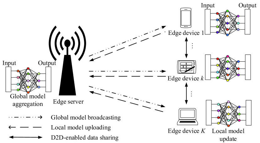
Figure 1: Illustration of the mobile edge learning system.

In this section, we introduce the distributed ML-model training in a mobile edge learning system. As shown in Figure 1, we consider a mobile edge learning system, which consists of an edge server and a set $\mathcal{K}\triangleq\{1,\ldots,K\}$ of edge devices. Suppose that each edge device $i\in\mathcal{K}$ has a set $\mathcal{D}_{i}$ of training data samples, where each data sample $d\in\mathcal{D}_{i}$ normally contains an input vector $\bm{x}_{d}$ and a desired output $y_{d}$. For each data sample, we define the corresponding loss function as $f(\bm{w},\bm{x}_{d},y_{d})$, abbreviated by $f_{d}(\bm{w})$, where $w$ denotes the ML-model parameter vector to be trained. By taking the convolutional neural network (CNN) as an example, the loss function $f_{d}(\bm{w})$ can be defined as the cross-entropy on cascaded linear and non-linear transforms [6]. Then, the local loss function at each edge device $i\in\mathcal{K}$ is given by $F_{i}(\bm{w})=\frac{\sum\limits_{d\in{\mathcal{D}_{i}}}{{f_{d}}({\bm{w}})}}{|\mathcal{D}_{i}|}$, where $|\mathcal{A}|$ denotes the cardinality of a set $\mathcal{A}$. Accordingly, the global loss function is $F(\bm{w})=\frac{\sum\limits_{i\in\mathcal{K}}{|\mathcal{D}_{i}|{F_{i}}({\bm{w}})}}{\sum\limits_{i\in\mathcal{K}}{|\mathcal{D}_{i}|}}$. The objective of mobile edge learning is to find the optimized parameter vector $\bm{w}^{*}$ that minimizes the global loss function $F(\bm{w})$, i.e.,

$$\bm{w}^{*}=\arg\min_{\mbox{\boldmath{$w$}}}F({\bm{w}}).$$ (1)

In order to solve problem (1) based on data samples distributed at the $K$ edge devices, we use the distributed batch gradient descent (BGD) method, which is implemented in an iterative manner and consists of four steps at each global iteration. In the following, we explain the detailed communication and computation process in each global iteration, respectively.

I) Global Model Broadcasting: In the first step of each global iteration, the edge server broadcasts the global parameter vector $w$ to all the $K$ edge devices for synchronization, i.e., each edge device $i\in\mathcal{K}$ updates its local model parameter vector as $\bm{w}_{i}=\bm{w}$. This step corresponds to the physical multicast channel in wireless communications [12]. Let $B$ denote the system bandwidth, $P_{s}$ denote the transmit power of edge server, and $g_{i}$ denote the channel power gain from the edge server to edge device $i\in\mathcal{K}$. Then the achievable data-rate throughput from the edge server to these edge devices is given by $r^{\text{(I)}}=\mathop{\min}\limits_{i\in\mathcal{K}}\{B{\log_{2}}(1+\frac{{{g_{i}}{P_{s}}}}{{{n_{0}}B}})\}$, where $\mathit{n_{0}}$ denotes the power spectral density (PSD) of the additive white Gaussian noise (AWGN) at the receiver of each edge device. Furthermore, let $Q$ denote the required number of bits for sending $w$, which generally depends on the quantization and compression methods used for encoding $w$. Accordingly, the time duration for global model parameters downloading at each global iteration is given by

$$t^{\text{(I)}}=\frac{Q}{\mathop{\min}\limits_{i\in\mathcal{K}}\{B{\log_{2}}(1+\frac{{{g_{i}}{P_{s}}}}{{{n_{0}}B}})\}}.$$ (2)

II) Local Model Update: After synchronizing the local model parameter vector, each edge device $i\in\mathcal{K}$ updates its local model parameter vector based on the gradient of the corresponding local loss function, i.e., $\bm{w}_{i}\leftarrow\bm{w}_{i}+\eta\nabla F_{i}(\bm{w}_{i})$, where $\eta>0$ denotes the learning rate, and $\nabla F_{i}(\bm{w}_{i})$ denotes the gradient of $F_{i}(\bm{w}_{i})$. In general, suppose that the local model update is operated over $N\geq 1$ (local) iterations to speed up the convergence by reducing the global iteration rounds. For such local model update at each edge device, we use the floating point operations (FLOPs) to measure the computation complexity, which generally depends on the considered ML-models and the size of parameter vector $w$. Without loss of generality, we denote the FLOPs needed for computing the gradient for each data sample in each local iteration as $L$. Therefore, the total FLOPs required for each edge device $i$ is approximated as $NL|\mathcal{D}_{i}|$, and accordingly the duration of local model update at edge device $i$ is given by

$$t^{\text{(II)}}_{i}=\frac{NL|\mathcal{D}_{i}|}{{{C_{i}}{f_{i}}}},$$ (3)

where $C_{i}$ denotes the FLOPs within a central processing unit (CPU) cycle and $f_{i}$ denotes the constant CPU frequency at each edge device $i\in\mathcal{K}$.

III) Local Model Uploading: After all edge devices finish the local model update, they upload their local parameter vectors to the edge server. This step corresponds to a wireless multiple access channel from the $K$ edge devices to the edge server. We employ the frequency division multiple access (FDMA) transmission protocol for local model uploading, in which each edge device $i\in\mathcal{K}$ uploads its individual local model parameter vector over an orthogonal frequency band. Let $\bar{b}_{i}\geq 0$ denote the allocated (optimizable) system bandwidth for edge device $i\in\mathcal{K}$. We thus have

$$\sum\limits_{i\in\mathcal{K}}{\bar{b}_{i}}\leq B.$$ (4)

Accordingly, the achievable data-rate throughput from edge device $i$ to the edge server is given by $r^{\text{(III)}}_{i}(\bar{b}_{i})=\bar{b}_{i}{\log_{2}}\big{(}1+\frac{{{{g_{i}}}{{P_{i}}}}}{{{n_{0}}\bar{b}_{i}}}\big{)}$, where $P_{i}$ denotes the transmit power of edge device $i$. The transmission duration for local model uploading at edge device $i$ is thus given by

$$t^{\text{(III)}}_{i}(\bar{b}_{i})=\frac{Q}{\bar{b}_{i}{\log_{2}}\big{(}1+\frac{{{{g_{i}}}{{P_{i}}}}}{{{n_{0}}\bar{b}_{i}}}\big{)}}.$$ (5)

IV) Global Model Aggregation: In the last step of the global iteration, the edge server obtains an updated parameter vector by aggregating the local models uploaded from edge devices, i.e., $\mbox{\boldmath{$w$}}\leftarrow\frac{{\sum\limits_{i\in\mathcal{K}}{\left|{{\mathcal{D}_{i}}}\right|{\bm{w}_{i}}}}}{{\sum\limits_{i\in\mathcal{K}}{\left|{{\mathcal{D}_{i}}}\right|}}}$. Notice that the edge server generally has huge computation power, and as a result, the global model aggregation can be accomplished within a negligible time duration (i.e., $t^{\text{(IV)}}\approx 0$).

As the above global iteration proceeds, the aggregated model parameter vector $w$ will converge towards a desirable value. Suppose that the above processes from step I) to IV) are operated over $M$ (global) iterations. Then, the total duration of ML-model training (or training delay) is given by

$$t(\{\bar{b}_{i}\})= M\Big{(}t^{\text{(I)}}+\mathop{\max}\limits_{\rm{\mathit{i}\in\mathcal{K}}}\{t^{\text{(II)}}_{i}+t^{\text{(III)}}_{i}(\bar{b}_{i})\}\Big{)}$$

$$= M\Big{(}\frac{Q}{\mathop{\min}\limits_{i\in\mathcal{K}}\{B{\log_{2}}(1+\frac{{{g_{i}}{P_{s}}}}{{{n_{0}}B}})\}}+$$

$$\mathop{\max}\limits_{\rm{\mathit{i}\in\mathcal{K}}}\left\{\frac{NL|\mathcal{D}_{i}|}{{{C_{i}}{f_{i}}}}+\frac{Q}{\bar{b}_{i}{\log_{2}}\big{(}1+\frac{{{{g_{i}}}{{P_{i}}}}}{{{n_{0}}\bar{b}_{i}}}\big{)}}\right\}\Big{)}.$$ (6)

As the edge devices are heterogeneous in computation and communication (i.e., $|\mathcal{D}_{i}|,C_{i},f_{i},g_{i},P_{i}$ are distinct over different edge devices), the computation and communication duration for step II) and III) (i.e., $t_{i}^{\text{(II)}}+t_{i}^{\text{(III)}}(\bar{b}_{i})$) is different for different edge devices. Therefore, the slowest edge device will fundamentally limit the total duration $t(\{\bar{b}_{i}\})$. This results in the so-called “straggler’s dilemma” issue.

III D2D-Enabled Data Sharing with Adaptive Radio Resource Allocation

In this section, we propose a D2D-enabled data sharing approach to deal with the “straggler’s dilemma” issue for reducing the training delay. In particular, an additional D2D-enabled data sharing phase is implemented before the above distributed ML-model training to adjust the number of data samples (or computation loads) among the $K$ edge devices for speeding up the computation.

III-A D2D-Enabled Data Sharing

In the D2D-enabled data sharing, different edge devices are enabled to exchange data samples among each other to adjust their computation loads based on their computation and communication capabilities. Let $\mathit{d_{ij}}$ $\geq 0,i,j\in\mathcal{K},j\neq i,$ denote the number of data samples transferred from edge device $\mathit{i}$ to edge device $\mathit{j}$. For each edge device $i$, we have

$$\sum\limits_{j\neq i}{{d_{ij}}}\leq|\mathcal{D}_{i}|,\forall i\in\mathcal{K}.$$ (7)

We consider that different D2D pairs are communicated over orthogonal frequency bands. Let $b_{ij}\geq 0,i,j\in\mathcal{K},j\neq i,$ denote the bandwidth allocated in the D2D communication from edge device $i$ to edge device $j$. We have

$$\sum\limits_{i\in\mathcal{K}}{\sum\limits_{j\neq i}{{b_{ij}}}}\leq B.$$ (8)

Let $p_{ij}\geq 0,i,j\in\mathcal{K},j\neq i,$ denote the transmit power at edge device $i$ for communicating with edge device $j$. Then we have

$$\sum\limits_{j\neq i}{{p_{ij}}}\leq{{P_{i}}},\forall i\in\mathcal{K}.$$ (9)

Consequently, the achievable D2D data-rate throughput from edge device $\mathit{i}$ to edge device $\mathit{j}$ is given by $r_{ij}({b_{ij}},{p_{ij}})=b_{ij}{\log_{2}}\big{(}1+\frac{{{h_{ij}}{p_{ij}}}}{{{n_{0}}b_{ij}}}\big{)}$, where $\mathit{h_{ij}}$ denotes the corresponding channel power gain. Accordingly, the transmission duration for edge device $\mathit{i}$ to transfer data to edge device $\mathit{j}$ is given as

$$t_{ij}({d_{ij}},{b_{ij}},{p_{ij}})=\frac{{a{d_{ij}}}}{b_{ij}{\log_{2}}\big{(}1+\frac{{{h_{ij}}{p_{ij}}}}{{{n_{0}}b_{ij}}}\big{)}},$$ (10)

where $a$ denotes the bits of each data sample. Therefore, we obtain the total time duration for data sharing as

$$t_{0}({\{d_{ij}},{b_{ij}},{p_{ij}}\})=\max_{i,j\in\mathcal{K},\atop\scriptsize j\neq i}\left\{\frac{{a{d_{ij}}}}{b_{ij}{\log_{2}}(1+\frac{{{h_{ij}}{p_{ij}}}}{{{n_{0}}b_{ij}}})}\right\}.$$ (11)

After finishing data sharing, the number of data samples at edge device $i\in\mathcal{K}$ is expressed as

$$|\mathcal{D}_{i}^{\prime}|=|\mathcal{D}_{i}|+\sum\limits_{j\neq i}{{d_{ji}}-\sum\limits_{j\neq i}{{d_{ij}}}},$$ (12)

where $\mathcal{D}_{i}^{\prime}$ denotes the updated data set at edge device $i$. In this case, the delay for each edge device $i$ to execute the local model update (Step II)) is revised as

$$\bar{t}^{\text{(II)}}_{i}({\{d_{ij}\}})=\frac{{NL({|\mathcal{D}_{i}|+\sum\limits_{j\neq i}{{d_{ji}}-\sum\limits_{j\neq i}{{d_{ij}}}}})}}{{{C_{i}}{f_{i}}}}.$$ (13)

Therefore, under D2D-enabled data sharing, the total time duration for the ML-model training or total training delay is given by

$$\bar{t}({\{d_{ij}},{b_{ij}},{p_{ij}},\bar{b}_{i}\})$$

$$= t_{0}\big{(}{\{d_{ij}},{b_{ij}},{p_{ij}}\}\big{)}+M\big{(}t^{\text{(I)}}+\mathop{\max}\limits_{\rm{\mathit{i}\in\mathcal{K}}}\{\bar{t}^{\text{(II)}}_{i}({\{d_{ij}\}})+t^{\text{(III)}}_{i}(\bar{b}_{i})\}\big{)}$$

$$= \max_{i,j\in\mathcal{K},\atop\scriptsize j\neq i}\left\{\frac{{a{d_{ij}}}}{b_{ij}{\log_{2}}(1+\frac{{{h_{ij}}{p_{ij}}}}{{{n_{0}}b_{ij}}})}\right\}+M\Big{(}\frac{Q}{\mathop{\min}\limits_{i\in\mathcal{K}}\{B{\log_{2}}\big{(}1+\frac{{{g_{i}}{P_{s}}}}{{{n_{0}}B}}\big{)}\}}+$$

$$\mathop{\max}\limits_{\rm{\mathit{i}\in\mathcal{K}}}\left\{\frac{{NL({|\mathcal{D}_{i}|+\sum\limits_{j\neq i}{{d_{ji}}-\sum\limits_{j\neq i}{{d_{ij}}}}})}}{{{C_{i}}{f_{i}}}}+\frac{Q}{\bar{b}_{i}{\log_{2}}\big{(}1+\frac{{{{g_{i}}}{{P_{i}}}}}{{{n_{0}}\bar{b}_{i}}}\big{)}}\right\}\Big{)}.$$ (14)

By comparing $\bar{t}({\{d_{ij}},{b_{ij}},{p_{ij}},\bar{b}_{i}\})$ in (III-A) versus $t(\{\bar{b}_{i}\})$ in (II), it is observed that the D2D-enabled data sharing can reshape the data samples at edge devices for reducing the computation delay at step II) at the cost of introducing an additional delay term $t_{0}({\{d_{ij}},{b_{ij}},{p_{ij}}\})$. Therefore, to minimize the total training delay, we need to design the data sharing $\{d_{ij}\}$ and the radio resource allocation $\{b_{ij},p_{ij},\bar{b}_{i}\}$ for balancing such a trade-off.

III-B Adaptive Radio Resource Allocation

In this subsection, we optimize the radio resource allocation for both D2D-enabled data sharing and distributed training to minimize the total training delay. For ease of notation, we define $v$ as a vector containing all the variables in $\{d_{ij},b_{ij},p_{ij},\bar{b}_{i}\}$, and we use $\mbox{\boldmath{$v$}}\succeq\mbox{\boldmath{$0$}}$ to denote that all these variables are non-negative. Therefore, the radio resource allocation problem for minimizing the training delay is formulated as

$$\text{(P1)}:\min_{\mbox{\boldmath{$v$}}\succeq\mbox{\boldmath{$0$}}}~{} \bar{t}({\{d_{ij}},{b_{ij}},{p_{ij}},\bar{b}_{i}\})$$ (15)

s.t. $$(\ref{bi}),(\ref{dij}),(\ref{bij}),(\ref{pij}).$$

Note that problem (P1) is generally challenging to be solved as the objective function in (15) is non-convex due to the coupling of $d_{ij}$, $b_{ij}$ and $p_{ij}$.

To solve problem (P1), we first introduce two auxiliary variables $\tau_{1}$ and $\tau_{2}$, and accordingly transform problem (P1) as the following equivalent problem:

$$\text{(P1.1)}:~{} \min_{\scriptsize\tau_{1},\tau_{2},\mbox{\boldmath{$v$}}}\tau_{1}+M(t^{\text{(I)}}+\tau_{2})$$ (16a)

s.t. $$\tau_{1}\geq 0,\tau_{2}\geq 0$$ (16b)

$$ad_{ij}\leq\tau_{1}b_{ij}{\log_{2}}\big{(}1+\frac{{{h_{ij}}{p_{ij}}}}{{{n_{0}}b_{ij}}}\big{)},\forall i,j\in\mathcal{K},j\neq i$$ (16c)

$$\bar{t}^{\text{(II)}}_{i}({\{d_{ij}\}})+t^{\text{(III)}}_{i}(\bar{b}_{i})\leq\tau_{2},\forall i\in\mathcal{K},j\neq i$$ (16d)

$$(\ref{bi}),(\ref{dij}),(\ref{bij}),(\ref{pij}).$$

Problem (P1.1) is still non-convex due to the coupling of $b_{ij}$ and $\tau_{1}$ in (16c). Nevertheless, notice that problem (P1.1) is a convex problem under any given $\tau_{1}$. Therefore, we propose to solve problem (P1.1) and thus (P1), by optimizing over $v$ and $\tau_{2}$ by using CVX [13] under any given $\tau_{1}$, and then using a one-dimensional (1D) search over $\tau_{1}$. During the 1D search, the regime of $\tau_{1}$ is set to be $[0,T_{1}]$, where $T_{1}$ is given in (III-B), which corresponds to the training delay under the case without data sharing and equal bandwidth allocation (i.e., $d_{ij}=0,\forall i,j\in\mathcal{K},i\neq j$, and $\bar{b}_{i}=\frac{B}{K}$).

$$T_{1}= M\Big{(}\frac{Q}{\mathop{\min}\limits_{i\in\mathcal{K}}\{B{\log_{2}}\big{(}1+\frac{{{g_{i}}{P_{s}}}}{{{n_{0}}B}}\big{)}\}}+$$

$$\mathop{\max}\limits_{\rm{\mathit{i}\in\mathcal{K}}}\left\{\frac{NL|\mathcal{D}_{i}|}{{{C_{i}}{f_{i}}}}+\frac{Q}{\frac{B}{K}{\log_{2}}\big{(}1+\frac{{{{g_{i}}}{{P_{i}}}}}{{{n_{0}}\frac{B}{K}}}\big{)}}\right\}\Big{)}.$$ (17)

Therefore, problem (P1) is finally solved optimally.

Remark III.1

It can be shown that at the optimal solution to (P1), we must have $d_{ij}^{*}\cdot d_{ji}^{*}=0,\forall i,j\in\mathcal{K},j\neq i$, since otherwise, we can always modify $\{d_{ij}\}$ to achieve the same data distribution but with shorter delay of $t_{0}\big{(}{\{d_{ij}},{b_{ij}},{p_{ij}}\}\big{)}$ for data sharing. This shows that the data sharing between any two edge devices must be unidirectional.

Remark III.2

It can also be shown that at the optimality of (P1), it must hold that $\bar{t}^{\text{(II)}}_{i}({\{d_{ij}^{*}\}})+t^{\text{(III)}}_{i}(\bar{b}_{i}^{*})=\bar{t}^{\text{(II)}}_{j}({\{d_{ji}^{*}\}})+t^{\text{(III)}}_{j}(\bar{b}_{j}^{*}),\forall i,j\in\mathcal{K},j\neq i$, since otherwise, we can further reduce the total training delay by adjusting the bandwidth and power allocations. This shows that under the adaptive radio resource allocation, all edge devices should finish their local model update and uploading at the same time for minimizing the overall training delay.

IV Numerical Results

In this section, we present numerical results to validate the performance of our proposed D2D-enabled data sharing design, as compared with the following two benchmark schemes.

• Conventional design with fixed radio resource allocation: In this scheme, no D2D-enabled data sharing is implemented with $d_{ij}=0,\forall i,j\in\mathcal{K},i\neq j$. In step III) at each global iteration, the edge devices upload their updated local ML-model parameters to the edge server under equal bandwidth allocation, i.e., $\bar{b}_{i}=\frac{B}{K},\forall i\in\mathcal{K}$. The corresponding training delay is given by $T_{1}$ in (III-B).

• Conventional design with adaptive radio resource allocation: In this scheme, no D2D-enabled data sharing is implemented. Adaptive radio resource allocation is implemented in step III) of each global iteration. Accordingly, the bandwidth allocation for minimizing the training delay is formulated as

  $$\text{(P2)}:\min_{\{\bar{b}_{i}\}}~{} t(\{\bar{b}_{i}\})$$

  s.t. $$(\ref{bi}),$$

  which can be transformed into a convex form similarly as for (P1) and then solved optimally via CVX.

In the simulation, we consider that there are $K=6$ edge devices, which are located at a distance of $350$ meters with the edge server. We consider the path loss model ${\beta_{0}}({d}/{d_{0}}){{}^{-\alpha}}$, where $\beta_{0}=-30$ dB denotes the path loss at the reference distance of $d_{0}=1$ m, $\alpha=3$ is the pathloss exponent and $d$ is the distance between the transmitter and the receiver. Unless otherwise stated, we set the transmit power of the edge server as $P_{\text{s}}=43$ dBm, the system bandwidth as $B=1$ MHz, and the noise PSD as $n_{0}=-130$ dBm/Hz. For edge devices, we set the number of FLOPs within a CPU cycle as $C_{1}=C_{2}=8$, $C_{3}=C_{4}=12$, $C_{5}=C_{6}=16$, the CPU frequency as $f_{1}=f_{2}=1.5$ GHz, $f_{3}=f_{4}=1.95$ GHz, $f_{5}=f_{6}=2.5$ GHz, and the transmit power as $P_{i}=33$ dBm$,\forall i\in\mathcal{K}$.

Furthermore, we consider that a CNN [14] is trained by using the distributed BGD. We consider the MNIST dataset [15], where each image has 784 pixels and a label. For the purpose of initial investigation, we quantize each pixel into 8 bits without data compression used. Furthermore, suppose that each label consists of 4 bits. Accordingly, we have $a=784\times 8+4=6,276$ bits for each data sample. We also quantize each element in the ML-model parameter vector into $8$ bits. It then follows from [16] that under our considered CNN model, we have $Q=3.2$ Gbits and $L\approx 6$ GFLOPs. Furthermore, we set the number of local iterations as $N=5$ and the learning rate as $\eta=0.01$.

In addition, we consider the non-IID data distribution. In the considered MNIST dataset, there are 10 different types of labels. Accordingly, we divide the MNIST dataset into 10 subsets, and choose 5,000 data samples for each edge device from only two different subsets.

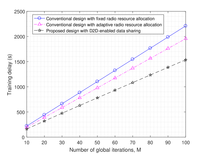
Figure 2: The total training delay versus the number of global iterations $M$.

Figure 2 shows the total time duration versus the number of global iterations $M$. It is observed that our proposed design with D2D-enabled data sharing achieves considerably shorter training delay than the two benchmark schemes. Such benefits are gained by reshaping the data distributions (and equivalently computation loads) among these devices, together with the adaptive radio resource allocation. Furthermore, such performance gain is observed to become more substantial as $M$ increases.

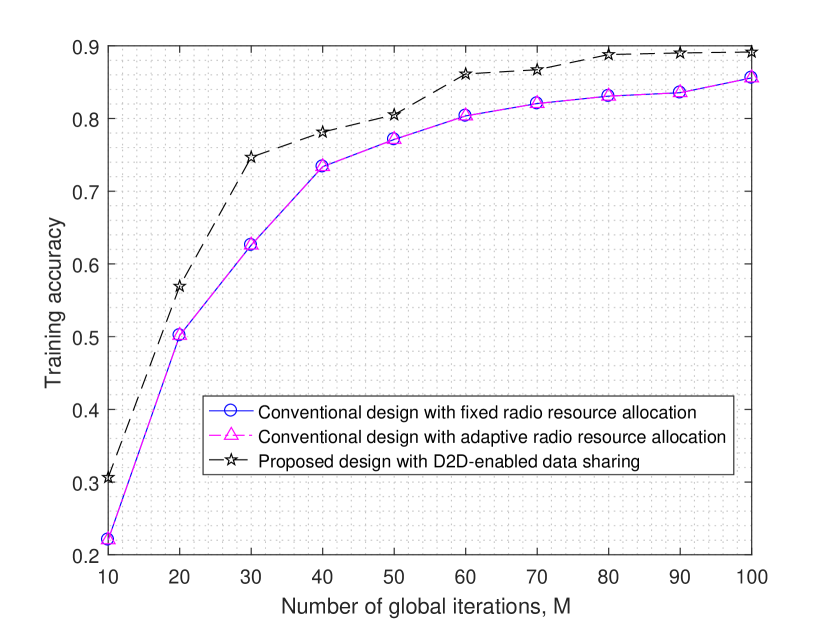
Figure 3: The training accuracy versus the number of global iterations $M$.

Figure 3 shows the training accuracy versus the number of global iterations $M$. It is observed that our proposed design with D2D-enabled data sharing achieves much higher training accuracy than the two benchmark schemes. This validates that the D2D-enabled data sharing is also beneficial in changing the data distribution among edge devices to resolve the non-IID distribution issue, thus improving the training accuracy.

V Conclusion

This letter proposed a D2D-enabled data sharing design for mobile edge learning, in which different edge devices can exchange their data samples among each other for reshaping the computation loads and data distributions. Under this setup, we proposed to optimize the adaptive radio resource allocation to minimize the total training delay. Numerical results showed that the proposed design not only improves the training speed, but also enhances the training accuracy, as compared to conventional designs without such consideration.

References

- [1] G. Zhu, D. Liu, Y. Du, C. You, J. Zhang, and K. Huang, “Towards an intelligent edge: Wireless communication meets machine learning,” to appear in IEEE Commun. Mag., 2019.
- [2] Q. Yang, Y. Liu, T. Chen, and Y. Tong, “Federated machine learning: Concept and applications,” ACM Trans. Intell. Syst. Technol., vol. 10, no. 2, pp. 1-19, Feb. 2019.
- [3] Y. Zhao, M. Li, L. Lai, N. Suda, D. Civin, and V. Chandra, “Federated learning with non-IID data.” [Online]. Available: http://arxiv.org/abs/1806.00582
- [4] F. Sattler, S. Wiedemann, K. Müller, and W. Samek, “Sparse binary compression: Towards distributed deep learning with minimal communication,” in Proc. IEEE IJCNN, 2019, pp. 1-8.
- [5] W. Wen, C. Xu, F. Yan, C. Wu, Y. Wang, Y. Chen, and H. Li, “TernGrad: Ternary gradients to reduce communication in distributed deep learning,” in Proc. NIP, 2017, pp. 1509-1519.
- [6] S. Wang, T. Tuor, T. Salonidis, K. K. Leung, C. Makaya, T. He, and K. Chan, “Adaptive federated learning in resource constrained edge computing systems,” IEEE J. Sel. Areas Commun., vol. 37, no. 6, pp. 1205-1221, Jun. 2019.
- [7] U. Mohammad and S. Sorour, “Adaptive task allocation for mobile edge learning,” in Proc. IEEE WCNCW, Apr. 2019, pp. 1-6.
- [8] G. Zhu, Y. Wang, and K. Huang, “Broadband analog aggregation for low-latency federated edge learning,” to appear in IEEE Trans. Wireless Commun., 2019.
- [9] L. Liu, J. Zhang, S. H. Song, and K. B. Letaief, “Edge-assisted hierarchical federated learning with non-IID data.” [Online]. Available: https://arxiv.org/abs/1905.06641
- [10] M. N. Tehrani, M. Uysal, and H. Yanikomeroglu, “Device-to-device communication in 5G cellular networks: Challenges, solutions, and future directions,” IEEE Commun. Mag., vol. 52, no. 5, pp. 86-92, May 2014.
- [11] D. Feng, L. Lu, Y. Yuan-Wu, G. Y. Li, G. Feng, and S. Li, “Device-to-device communications underlaying cellular networks,” IEEE Trans. Commun., vol. 61, no. 8, pp. 3541-3551, Aug. 2014.
- [12] N. D. Sidiropoulos, T. N. Davidson, and Z.-Q. Luo, “Transmit beamforming for physical-layer multicasting,” IEEE Trans. Signal Process., vol. 54, no. 6, pp. 2239-2251, Jun. 2006.
- [13] M. Grant, S. Boyd, and Y. Ye, “CVX: Matlab software for disciplined convex programming,” version 2.1, Mar. 2017. [Online]. Available: http://cvxr.com/cvx/
- [14] H. B. McMahan, E. Moore, D. Ramage, S. Hampson, and B. A. Arcas, “Communication-efficient learning of deep networks from decentralized data,” in Proc. AISTATS, 2017, pp. 1273-1282.
- [15] Y. Lecun, C. Cortes, and C. J. C. Burges, “The MNIST database of handwritten digits.” [Online]. Available: http://yann.lecun.com/exdb/mnist/
- [16] X. Giró-i-Nieto, E. Sayrol, A. Salvador, J. Torres, E. Mohedano, and K. McGuinness, Memory usage and computational considerations, Course Notes, accessed on Jul. 5 2016. [Online]. Available: http://imatge-upc.github.io/telecombcn-2016-dlcv/slides/D2L1-memory.pdf