Effects of Inertia, Load Damping and Dead-Bands on Frequency Histograms and Frequency Control of Power Systems

Abstract

The increasing penetration of renewable energy sources has been leading to the progressive phase-out of synchronous generators, which constitute the main source of frequency stability for electric power systems. In the light of these changes, over the past years, some power systems started to exhibit an odd frequency distribution characterised by a bimodal behavior. This results in increased wear and tear of turbine governors and, in general, in degraded frequency performances. This is a cause of concern for grid operators, which have become increasingly interested in understanding the factors shaping frequency distribution. This paper explores the root causes of unwanted frequency distributions. The influence of some main aggregate system parameters on frequency distribution is detailed. The paper also shows that the implementation of the so-called synthetic inertia can lead to a robust unimodal frequency distribution.

I Introduction

In electric power systems, frequency is the most important parameter that transmission system operators (tsos) must control and manage, trying to limit its variations within strict bounds [1]. Several corporations, as the North American Electric Reliability Corporation (NERC) [2], prepared documents concerning the decreasing trend in the frequency quality of a complex power system [3]. To solve this issue, some counteractions and remedies have been proposed, e.g., new settings for traditional generators dead-bands and droop gains [2], the exploitation of renewable energy sources (res) [4] and storage systems for frequency regulation services [5], demand response, the introduction of load and generation aggregators, and the adoption of thermostatically controlled loads, which can implement controllers that link the absorbed power to frequency variations and can mimic an inertial response. [6]. There is quite a large consensus that the main reason for this trend is the continuous reduction of system inertia, which is primarily due to the increasing penetration of res and converter-interfaced loads [7]. The focus is on these components since they deliver/absorb power regardless of frequency variations, thereby constituting frequency-independent generators/loads. The general indication is that the decrease in system inertia has to be restored in some way as the number of conventional synchronous generators are replaced by res [8]. For instance, this could be done by implementing the so-called synthetic (or virtual) inertia in converter-interfaced equipment, which allows mimicking the frequency response of synchronous generators following power imbalances [9]. While on the one hand, the factors determining the frequency behavior following a power disturbance are already well established, on the other hand the analysis of the parameters shaping power system frequency distribution due to the presence of stochastic load variations is still at an early stage of research. Early papers and reports addressing this topic showed that frequency distributes around its nominal value in a way that leads to bimodal histograms, which are characterised by two frequency occurrence peaks, often located almost symmetrically around the nominal frequency value. Such an odd frequency behavior has been reported in North America [10], Ireland [11], and, lastly, Great Britain [12], whose frequency measurement data are publicly available in [13]. This bimodal behavior is in contrast to the assumption typically put forward for the design of system controllers and statistical analysis, according to which frequency distribution is unimodal. Moreover, as shown in the following, it can cause an increased tear and wear of turbine governors. As a consequence, such a distribution is undesirable.

I-A Contributions

Starting from these considerations, we investigate and identify the reasons that lead to unwanted frequency distributions such as bimodal frequency histograms. This is initially done analytically through a formal approach applied to a simplified, linear power system model comprising a stochastic load [14], which constitutes the source of power mismatches. We then use a modified version of the well-known ieee 14 bus power system as a benchmark. Detailed numerical simulations are performed to compute frequency distributions in different operating scenarios. When possible, results are compared with experimental measurements of more complex power systems.

Some considerations and guidelines on how to act on power systems to avoid a bimodal frequency distribution are proposed. These considerations take into account effects due to dead-bands of turbine governors, automatic generation control (agc), the inertia of synchronous generators, variability, and stochastic characteristics of loads and generation, elements with power versus frequency dependence (e.g., frequency-dependent loads) and possibly synthetic inertia.

The main results we show are: (i) simply increasing or restoring inertia without considering the aggregate value of the load damping parameter can be ineffective. This is in contrast to the common belief that an increase in inertia is beneficial per se. (ii) Bimodal frequency distribution histograms are due to at least two remarkably different reasons. The former is an inappropriate procedure to aggregate frequency samples that simply leads to an “artifact” [12]. The latter is due to the adoption of ineffective dead-bands, as well as of an unsuitable choice of the values of other system parameters, which lead to continuous wear and tear of tgs and poorly-controlled swings following long-term, small power imbalances. (iii) The introduction of adequate controllers in electronically-interfaced loads and res generation can sensibly and beneficially modify the aggregate values of system parameters and mainly load damping and inertia. We show that this leads to very narrow, unimodal frequency distributions.

II Simplified model of a power system with stochastic load

Let us assume to have a simplified and linear power system model. In such a system, we consider $\Delta\omega$ as the deviation from $1\,\text{[pu]}$ of the angular frequency of the center of inertia (coi). We model it through the swing equation

$$2H\frac{d\Delta\omega}{dt}=-D_{\mathrm{L}}\Delta\omega-\eta(t)~{},$$ (1)

where $H$ is the inertia of the coi and $D_{\mathrm{L}}$ is the load damping coefficient. We assume that the $\eta(t)$ power fluctuations in the swing equation are due to a stochastic load, modeled by the linear stochastic differential equation

$$d\eta=\left(\mu-\alpha\eta(t)\right)dt+b\,dW_{t}~{},$$ (2)

where $\alpha$ is known as the reciprocal of the load reversal time, $b$ governs the variance of $\eta(t)$ and $W_{t}$ is a scalar Wiener process. The use of a stochastic model of power loads is not novel; see for example [15, 16, 17].

The choice of a linear model is plausible when the dead-bands of tgs are wide enough with respect to the frequencies deviations caused by the stochastic load. If so, the intervention of tgs is prevented. Furthermore, when the stochastic load leads to modest frequency variations, a linearised version of a complex non-linear power system can be employed. The linear model in (1) is based on the coi and considers an aggregate, unique swing equation [12, 1].

Equations (1) and (2) can be written in compact form as

$$\left[\begin{IEEEeqnarraybox}[]{[}][c]{,c,}d\Delta\omega\\ d\eta\end{IEEEeqnarraybox}\right]=\left[\begin{IEEEeqnarraybox}[]{[}][c]{,c,}0\\ \mu\end{IEEEeqnarraybox}\right]dt-\left[\begin{IEEEeqnarraybox}[]{[}][c]{,c/c,}\frac{D_{\mathrm{L}}}{2H}&\frac{1}{2H}\\ 0&\alpha\end{IEEEeqnarraybox}\right]\left[\begin{IEEEeqnarraybox}[]{[}][c]{,c,}\Delta\omega\\ \eta\end{IEEEeqnarraybox}\right]dt+\left[\begin{IEEEeqnarraybox}[]{[}][c]{,c,}0\\ b\end{IEEEeqnarraybox}\right]d{W}_{t}~{}.$$ (3)

Eq. (3) belongs to the general class of multi-dimensional linear stochastic equations in the form [18]

$$d\mathbf{x} =\left(\boldsymbol{\mu}(t)-\mathbf{A}\right)\mathbf{x}\,dt+\mathbf{B}\,d\mathbf{W}_{t}$$ (4)

$$\mathbf{x}(t_{0}) =\mathbf{x}_{o}~{},$$

where $\mathbf{W}_{t}$ is an $M$-dimensional Wiener process, $\mathbf{A}\in\mathds{R}^{N\times N}$, $\mathbf{B}\in\mathds{R}^{N\times M}$ are constant matrices, $\boldsymbol{\mu}(t)$ is an $N$-dimensional vector of time functions, and $\mathbf{x}_{o}$ is the initial condition. Equation (4) admits the solution

$$\mathbf{x}(t)=e^{-\mathbf{A}(t-t_{0})}\mathbf{x}_{o}+\!\!\int_{t_{0}}^{t}{\!\!e^{-\mathbf{A}(t_{0}-s)}\!\left(\boldsymbol{\mu}(s)ds+\!\mathbf{B}d\mathbf{W}_{s}\right)}~{},$$ (5)

and

$$\mathrm{E}\left[\mathbf{x}(t)\right]=e^{-\mathbf{A}(t-t_{0})}\left(\mathrm{E}[\mathbf{x}_{o}]+\int_{t_{0}}^{t}{\!\!e^{-\mathbf{A}(t_{0}-s)}\boldsymbol{\mu}(s)ds}\right)~{}.$$ (6)

Without loss of generality, in the following we assume $t_{0}=0$ and $\mathrm{E}[\mathbf{x}_{o}]=0$.

The covariance matrix of $\mathbf{x}(t)$ is the solution of the

$$\dot{\mathbf{w}}=-\left(\mathbf{A}\mathbf{w}+\mathbf{w}\mathbf{A}^{\mathrm{T}}\right)+\mathbf{B}\mathbf{B}^{\mathrm{T}}$$ (7)

differential equation (the $\mbox{}^{\mathrm{T}}$ super-script denotes transposition). In our analysis, we focused on (3) letting both ${\mu}$ constant and ${\mu(t)=\rho\sin(\Psi t)}$. In the first case, (2) models the evolution of the Ornstein-Uhlenbeck process [19], which is exponentially-autocorrelated and normally-distributed, with $\displaystyle{\mathrm{E}[\eta(t)]=\nicefrac{{\mu}}{{\alpha}}+\left(\eta(0)-\nicefrac{{\mu}}{{\alpha}}\right)e^{-\alpha t}}$ time-varying mean and

$$\mathrm{Var}[\eta(t)]=\frac{b^{2}}{2\alpha}\left(1-e^{-2\alpha t}\right)$$ (8)

time-varying variance. $\eta(t)$ asymptotically tends to ${\nicefrac{{\mu}}{{\alpha}}}$ as $t$ tends to infinity. Since, in particular, we assume ${\mu}=0$, as far as $\alpha t\gg 0$ the stochastic load on average does not contribute power and ${\mathrm{E}}[\Delta\omega]_{\alpha t\gg 0}$ is null too.

In the second case, $\mu(t)$ is used to model a slowly-varying deterministic and periodic (daily) power imbalance. We assume ${\Psi\ll 2\pi\alpha}$, viz. the period of $\mu(t)$ is much larger than the process reversal-time. By exploiting (6) with $2H\alpha\neq D_{\mathrm{L}}$ we get

$$\begin{array}[]{lcl}{\mathrm{E}}[\Delta\omega]&\!\!=\!\!&\displaystyle{ke^{-\frac{D_{\mathrm{L}}}{H}t}+\frac{\rho\Psi e^{-\alpha t}}{\left(\alpha^{2}+\Psi^{2}\right)\left(2H\alpha-D_{\mathrm{L}}\right)}~{}+}\\[8.53581pt] &\!\!+\!\!&\displaystyle{\rho_{c}\cos\left(\Psi t\right)+\rho_{s}\sin\left(\Psi t\right)}\end{array}~{},$$ (9)

where

$$\begin{array}[]{l}\displaystyle{\rho_{c}=\frac{\rho\Psi\left(2H\alpha+D_{\mathrm{L}}\right)}{\left(4H^{2}\Psi^{2}+D_{\mathrm{L}}^{2}\right)\left(\alpha^{2}+\Psi^{2}\right)}}\\[8.53581pt] \displaystyle{\rho_{s}=\frac{\rho\left(2H\Psi^{2}-\alpha D_{\mathrm{L}}\right)}{\left(\alpha^{2}+\Psi^{2}\right)\left(4H^{2}\Psi^{2}+D_{\mathrm{L}}^{2}\right)}}\end{array}$$

and $k$ is chosen to guarantee that $\mathrm{E}[\Delta\omega(0)]=0$. By solving (7) the expression of the variance of $\Delta\omega$ is

$$\mathrm{Var}[\Delta\omega]\!=\!\sigma^{2}\!\left(1\!-\!\kappa_{1}e^{-\frac{D_{\mathrm{L}}}{H}t}\!+\!\kappa_{2}e^{-\frac{D_{\mathrm{L}}+2H\alpha}{2H}t}\right)\!-\!\kappa_{3}e^{-2\alpha t}~{},$$ (10)

where

$$\sigma=\frac{b}{\sqrt{2\alpha D_{\mathrm{L}}\left(D_{\mathrm{L}}+2H\alpha\right)}}$$ (11)

and

$$\begin{array}[]{l}\displaystyle{\kappa_{1}=\frac{2H\alpha\left(D_{\mathrm{L}}+2H\alpha\right)}{\left(D_{\mathrm{L}}-2H\alpha\right)^{2}}}\\[11.38109pt] \displaystyle{\kappa_{2}=\frac{8H\alpha D_{\mathrm{L}}}{\left(D_{\mathrm{L}}-2H\alpha\right)^{2}}}\\[8.53581pt] \displaystyle{\kappa_{3}=\frac{b^{2}}{2\alpha\left(D_{\mathrm{L}}-2H\alpha\right)^{2}}}~{}.\end{array}$$

An important aspect is that $\boldsymbol{\mu}(t)$ does not appear in (7), thus $\mathbf{w}(t)$ does not depend on it. Consequently, (11) is invariant w.r.t. ${\mu}(t)$. When $t$ is sufficiently large, (9) and (10) simplify as

$$\mathrm{E}[\Delta\omega]_{\alpha t\gg 0}\simeq\rho_{c}\cos\left(\Psi t\right)+\rho_{s}\sin\left(\Psi t\right)~{},$$ (12)

viz. a periodic function with period equal to $\nicefrac{{2\pi}}{{\Psi}}$, and

$$\mathrm{Var}[\Delta\omega]_{\alpha t\gg 0}\simeq\sigma^{2}~{}.$$ (13)

By observing (11), we see that $\sigma$ is a constant which is inversely proportional to the ${D_{\mathrm{L}}}$ load damping, to the $\nicefrac{{1}}{{\alpha}}$ load reversal time, and the $H$ inertia. It is worth pointing out that the $H$ inertia is multiplied by $\alpha$ at the denominator of $\sigma$ and then by $D_{\mathrm{L}}$. This means that the smaller $D_{\mathrm{L}}$, the lower the effectiveness of inertia in limiting frequency deviations. This is in contrast to the common idea that an increment of the overall system inertia is beneficial, regardless of the value of other aggregate system parameters. From our standpoint, this is a relevant result. We will consider this matter in further detail in the following.

Another aspect is that $D_{\mathrm{L}}$ adds to $2H\alpha$ and it is thus deemed to play a significant role in limiting frequency variations. In the light of this, $D_{\mathrm{L}}$ could be increased by exploiting thermostatically controlled loads that link frequency variations to the absorbed power [20, 21, 22, 23, 24], as anticipated in the Introduction, as well as load damping and synthetic inertia, which require a suitable implementation of res generation and storage systems [25, 26, 27].

We pay now some more attention to $\sigma$. As $D_{\mathrm{L}}$ tends to $0$, $\sigma$ increases, i.e., the distribution of $\Delta\omega$ around $0$ flattens and extends. Thus, as shown in the following, the reduction of $D_{\mathrm{L}}$ leads to an increased probability of crossing the dead-bands implemented in tgs. The variance of $\Delta\omega$, in the extreme case when $D_{\mathrm{L}}=0$, is

$$\mathrm{Var}[\Delta\omega]_{D_{\mathrm{L}}=0}=\frac{b^{2}}{4H^{2}\alpha^{2}}\!\left[t\!+\!\frac{1}{\alpha}\!\!\left(2e^{-\alpha t}\!-\frac{1}{2}e^{-2\alpha t}\!-\frac{3}{2}\right)\!\right]~{}.$$ (14)

This expression clearly shows that $\mathrm{Var}[\Delta\omega]_{D_{\mathrm{L}}=0}$ increases with time. As a consequence, the probability that dead-bands are crossed increases with time too. When $t$ is sufficiently large so that $\alpha t$ is far larger than 0, the two exponential terms in (14) are practically 0 and

$${\mathrm{Var}[\Delta\omega]_{D_{\mathrm{L}}=0,\alpha t\gg 0}\,\simeq\,\frac{b^{2}}{4H^{2}\alpha^{2}}\left(t-\frac{3}{2\alpha}\right)}~{}.$$ (15)

It means that, at least in the simplified model of the power system, if $D_{\mathrm{L}}=0$, by acting on the system inertia alone, the frequency is likely to trespass the bounds of the dead-bands of the tgs, anyway. It is the first relevant result of the paper. We dare say that this is in contrast to the common belief that a sufficiently high increase of the aggregate system inertia (coi inertia) is always beneficial to lower frequency variations. It seems false with stochastic loads. We come back on this aspect in Section V.

III Numerical simulation setup

As previously said, the simplified model described by (3) may grab the main features of a complex non-linear power system model that works in suitable conditions. To show what happens to frequency when a complex power system is stimulated by loads modeled as stochastic and how frequency depends on system settings and aggregated parameters, we resort to numerical simulations and elect the well known ieee 14 bus power system to the role of our benchmark. Since the insight coming from (3) has general validity, we could have chosen other known power system models than the ieee 14 bus power system.

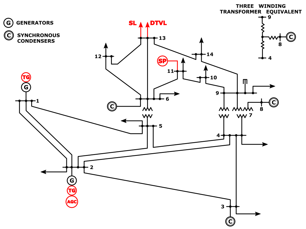
Figure 1: One-line diagram of the modified ieee 14-bus system. g: generator. c: synchronous condenser. tg: turbine governor. agc: automatic generation control. sl: stochastic load. dtvl: daily time-varying load. sp: solar plant. The parameter values of the standard ieee 14-bus system can be found in [29] (see Chapter 21.4).

In the following, the ieee 14 bus power system is extended with several additions (see Fig. 1), which are used in different ways and scenarios depending on the factors shaping frequency deviations that we want to highlight.

• Each of the two generating units of the ieee 14 bus power system is equipped with a tg, whose control scheme is modified by including a dead-band block (see Fig. 2).

  

  Figure 2: Schematic of a tg with dead-band. The $d_{\mathrm{za}}$ value corresponds to the frequency threshold above which the tg modifies the generator power output. the state space model that implements the transfer function of the tg can be found in [30].

  Dead-bands are enabled/disabled according to the specific features that simulations aim at highlighting. As it is well known, dead-bands are implemented to prevent tgs from relentlessly operating even following small power variations. In principle, this insertion should not degrade the almost-Gaussian distribution of frequency around the nominal value.

• An additional stochastic load is connected to bus13. It is modeled as $\displaystyle{p_{\mathrm{L}}(t)=\eta(t)\,P_{\mathrm{L0}}\left(\frac{\left|v(t)\right|}{V_{0}}\right)^{\gamma}}\rule{0.0pt}{19.91692pt}$ [14, 30], where $P_{\mathrm{L0}}$ is the nominal active power of the load, $V_{0}$ is the load voltage rating, $v(t)$ is the bus voltage at which the load is connected, $\gamma$ governs the dependence of the load on bus voltage [30]. Load active power is ruled by the $\eta(t)$ Ornstein-Uhlenbeck’s process in (2) with ${\eta(0)=0}$, ${\alpha=0.5}$, ${b=1}$, ${\mu=0}$ [14]. This choice leads to a stochastic load that on average does not absorb active power. The purpose of this setup is to stimulate the power system and its controllers with a continuous active power disturbance. Two different values of $P_{\mathrm{L0}}$, namely $1\,\mathrm{M}\mathrm{W}$ and $10\,\mathrm{M}\mathrm{W}$, are considered.

• The conventional load of the ieee 14 bus system connected at bus13, which has $P_{\mathrm{D0}}=14.9\,\mathrm{M}\mathrm{W}$ nominal power, is replaced by the daily time-varying load

  $${p_{\mathrm{D}}(t)=P_{\mathrm{D0}}\left(1+\Delta p_{\mathrm{D}}(t)\right)\left(\frac{\left|v(t)\right|}{V_{0}}\right)^{\gamma}}~{},$$

  where

  $$\Delta p_{\mathrm{D}}(t)=-0.12\sin\left(\frac{t}{24\times 3600}\right)~{}\text{[pu]}~{}.$$ (16)

  In the conventional ieee 14 bus without dead-bands, the addition of this daily time-varying load causes the corresponding slow intervention of the tgs to balance the power mismatch. Frequency deviates from its nominal value of a very small amount due to the overall low power variation of the drifting load. As shown in the following, the effect of this drifting load on frequency distribution significantly changes when dead-bands are introduced.

• To compensate the slowly daily drifting power introduced above, we add a simple agc model as described in [1, 11]. The tg of generator g2 in the ieee 14 bus test system is driven by a simple agc described by the equation $\dot{P}_{\mathrm{agc}}=k_{\mathrm{agc}}\left(1-\omega_{\mathrm{acg}}\right)$. In our implementation, $\omega_{\mathrm{acg}}$ is the angular frequency of the coi and the agc output $P_{\mathrm{agc}}$ drives the ${\tt d_{p}}$ terminal of the summation block of the tg schematic shown in Fig. 2.

  The choice of adequate agc parameters and tgs dead-bands to avoid wear and tear may be a difficult task [31]. In any case, regardless of dead-bands, the action of the agc should be very slow and immune from fast frequency fluctuations due to stochastic loads with relatively short reversal time as in our case.

In every simulated scenario, we always performed an eigenvalue analysis after the computation of the power-flow solution to assess whether the modified system remained stable despite the additions above [30, 29, 1]. We also assume that the modified ieee 14 bus power system is ergodic, stationary, or cyclo-stationary. The Ornstein-Uhlenbeck’s process can be assumed stationary or cyclo-stationary if we consider its behavior for $\alpha t\gg 0$, as we do in all scenarios. Ergodicity allows us to substitute a set of relatively short time-domain simulations with a single long-lasting time-domain simulation to derive statistical properties. The samples of the $\eta(t)$ random variables were generated according to the mean and variance of the Ornstein-Uhlenbeck Gaussian process. $\eta(t)$ is thus transformed in a discrete box-car function on the $1\,\mathrm{s}$ evenly spaced time grid. Since the $\eta(t)$ samples can be computed before starting the simulation, we solved a random differential equation.

In the various scenarios, we simulate the ieee 14 bus power system for at least 24 hours after a sufficiently large setup time interval. We pick a frequency sample every $1\,\mathrm{s}$, thereby collecting $3600\times 24=86400$ samples of the frequency variations of the rotor speed of synchronous generators.

IV Frequency deviations

In this section, we consider several scenarios with different settings of the main system’s parameters, namely the $H$ inertia of the synchronous generators, the ${D_{\mathrm{L}}}$ load damping, and dead-bands. Each subsection considers a peculiar scenario, and we display the obtained results, i.e., frequency deviations, through histograms. Our target is to show, through this guided sequence of tailored simulations of a complex and general system like the ieee 14 bus one, how the link between $H$ and ${D_{\mathrm{L}}}$ in (11) and (14) can be exploited to understand their effects on frequency deviations and possibly how to limit frequency deviations. Table I gives a synoptic view of the ieee 14 bus system setups, used to derive all the histograms in the paper.

TABLE I: Synoptic setup of the histograms. Symbol $\bullet$ means selected.

To have a reference scenario for frequency deviations and to allow further easy comparisons, we firstly simulate the nominal ieee 14 bus system by adding the stochastic load only. The histogram of frequency deviations obtained in this case is reported in Fig. 3 [\raisebox{-.9pt} {a}⃝].

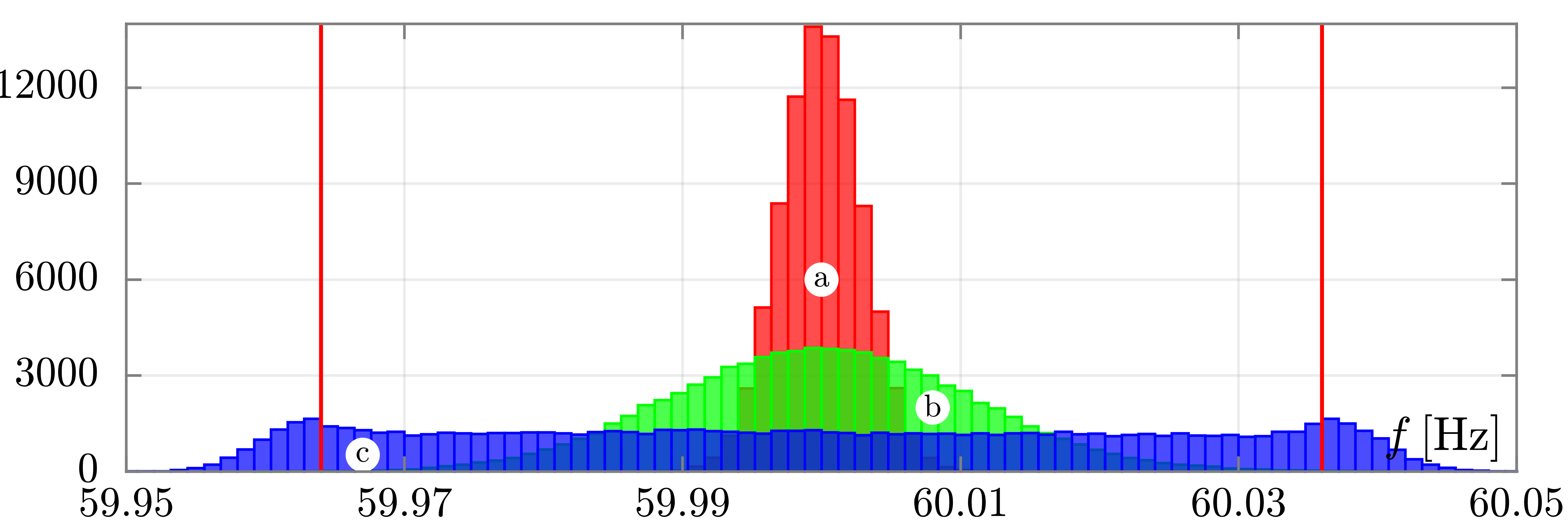
Figure 3: The \raisebox{-.9pt} {a}⃝ histogram shows the frequency deviations at nominal conditions and parameters of the ieee 14 bus power system. The \raisebox{-.9pt} {b}⃝ histogram refers to the case with dead-bands and the \raisebox{-.9pt} {c}⃝ one refers to the case with dead-bands and with $D_{\mathrm{L}}=0$. Vertical lines show the $\mathrm{d_{za}}$ frequency limits of the dead-band (see Fig. 2). All histograms are displayed with an equal number of bins (same width). Histograms report the number of occurrences in each bin. The value of $P_{\mathrm{L0}}$ is $1\,\mathrm{M}\mathrm{W}$.

The continuous intervention of the tgs, regulating the mechanical power from the prime movers that drive the two synchronous generators, leads to a quite limited frequency variation, which is also due to the modest variance of the stochastic load. The resulting frequency histogram is Gaussian. The frequency deviations with $P_{\mathrm{L0}}=10\,\mathrm{M}\mathrm{W}$ are still limited and are thus not reported. However, these settings have the disadvantage of requiring the continuous intervention of tgs, which is undesirable.

IV-A tg with dead-bands

We set up a new scenario that adds dead-bands to tgs by setting $d_{\mathrm{za}}=720\times 10^{-6}\,\text{[pu]}$ ($36\,\mathrm{m}\mathrm{Hz}$) in the block shown in the schematic of Fig. 2. The dead-band equally extends of the $d_{\mathrm{za}}$ amount around the center frequency. We chose this value since it is compliant with the standards in [3], i.e., it has practical ground. We simulate the power system for 24 hours. In the resulting frequency histogram (see the \raisebox{-.9pt} {b}⃝ histogram in Fig. 3), almost all of the frequency deviation occurrences lay inside the dead-band, whose thresholds are identified by vertical solid red lines in Fig. 3. It can be seen that in a complex power system there is a relation in limiting frequency variations linking the variance of the stochastic model of the loads, the extension of the dead-bands, and the fraction of tgs equipped with dead-bands with respect to those without dead-bands.

An interesting result is the \raisebox{-.9pt} {c}⃝ histogram shown in Fig. 3. It is obtained with dead-bands and with ${D_{\mathrm{L}}=0}$, i.e., by fictitiously assuming no dependence of the load power from frequency as if, for example, each induction motor were equipped with an electronic controller that decouples it from the grid, i.e., it keeps its rotor speed independent from grid frequency. We see an almost flat portion of the histogram inside the dead-band as predicted by (13) and (14). There is a modest increase of occurrences just outside the dead-band where the power fluctuations activate the tgs. When frequency exceeds the dead-band, tgs activate and pull frequency back. We recall that the power-flow solution in normal operating conditions gives a total active power absorbed by loads equal to $259\,\mathrm{M}\mathrm{W}$. When we set $P_{\mathrm{L0}}=1\,\mathrm{M}\mathrm{W}$, this value is about $0.4\%$ of the total active load power. This power variation, albeit small, leads to frequency fluctuations that are sufficiently large to trigger the intervention of tgs. Since we use a low-pass filtered white Gaussian source with variance given by (8) (recall that we set $b=1$ and $\alpha=0.5$) we tested the stability of the ieee 14 bus power system with a maximum power variation of $\pm 5P_{\mathrm{L0}}=\pm 5\times 10\mathrm{M}\mathrm{W}$. This corresponds to the $\mathrm{erf}\left(\frac{5}{\sqrt{2}}\right)\simeq 1-5.7330\times 10^{-7}$ expected fraction of the generated samples that fall inside the $\pm 5P_{\mathrm{L0}}$ interval. We expect that the ieee 14 bus power system almost always works in a stable condition. This removes the suspect that the frequency deviations are due to the system being unstable. The first consideration about the \raisebox{-.9pt} {c}⃝ histogram is that the complete elimination of any dependence of the power from frequency, i.e., the setting of ${D_{\mathrm{L}}=0}$, defeats the purpose of inserting dead-bands to limit wear and tear of tgs. This also largely justifies our choice of frequency dead-bands. We stress that an unaware and independent selection of the dead-band settings from the aggregate $D_{\mathrm{L}}$ value of a power system might be useless. The second consideration is that frequency distribution greatly deteriorates. We see that the shape of the histogram largely differs from a Gaussian one since it is practically flat inside the dead-band. This means that frequency uniformly fluctuates inside the dead-band. We performed several simulations by progressively lowering $D_{\mathrm{L}}$ from 2 to 0.

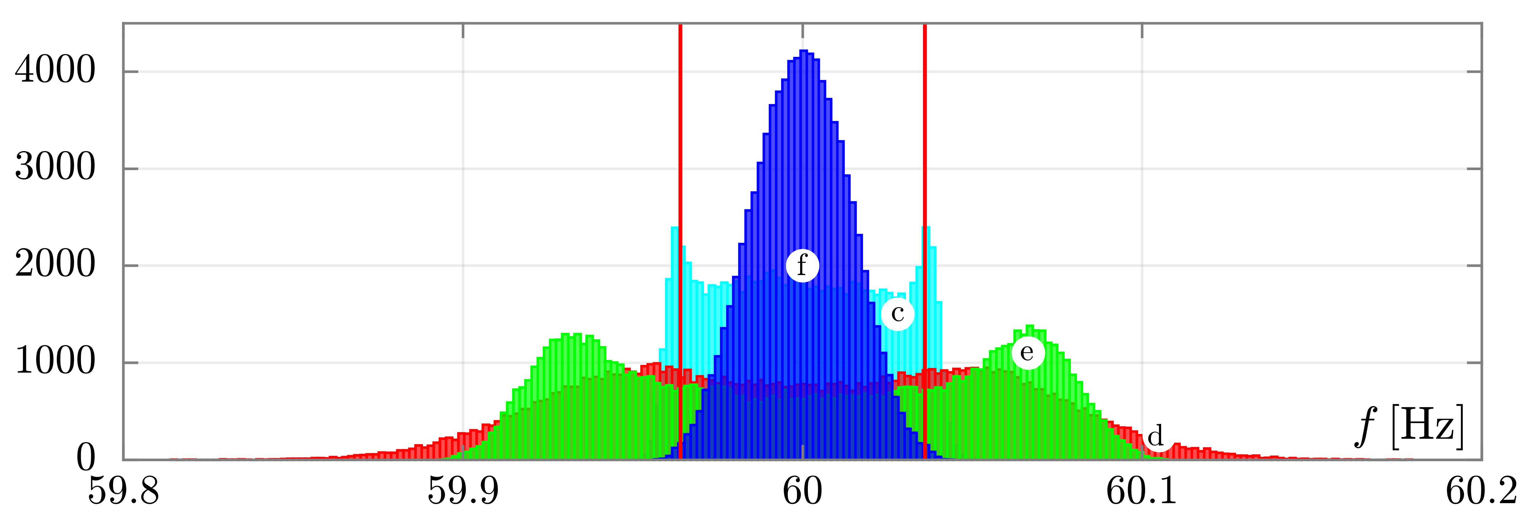
Figure 4: Frequency histograms. \raisebox{-.9pt} {c}⃝ histogram: $\mathrm{d_{za}}=36\,\mathrm{m}\mathrm{Hz}$, $D_{\mathrm{L}}=0$ and $P_{\mathrm{L0}}$ is $1\,\mathrm{M}\mathrm{W}$. \raisebox{-.9pt} {d}⃝ histogram: $\mathrm{d_{za}}=36\,\mathrm{m}\mathrm{Hz}$, $D_{\mathrm{L}}=0$ and $P_{\mathrm{L0}}$ is $10\,\mathrm{M}\mathrm{W}$. \raisebox{-.9pt} {e}⃝ histogram: $D_{\mathrm{L}}=2.0$, $\mathrm{d_{za}}=100\,\mathrm{m}\mathrm{Hz}$ $P_{\mathrm{L0}}=1\,\mathrm{M}\mathrm{W}$, power drifting is introduced (see Eq. (16)). The \raisebox{-.9pt} {c}⃝, \raisebox{-.9pt} {d}⃝, and \raisebox{-.9pt} {e}⃝ histograms are bimodal. The \raisebox{-.9pt} {f}⃝ histogram refers to the same scenario of the \raisebox{-.9pt} {e}⃝ one but with the introduction of the agc ($k_{\mathrm{agc}}=0.01$) that drives the tg of the g2 generator and with $\mathrm{d_{za}}=36\,\mathrm{m}\mathrm{Hz}$. Vertical lines mark the extension of the dead-band corresponding to the \raisebox{-.9pt} {d}⃝ and \raisebox{-.9pt} {f}⃝ histograms.

We do not report them due to space reasons. What we obtained is that by starting from the \raisebox{-.9pt} {b}⃝ histogram, the other histograms progressively flatten as $D_{\mathrm{L}}$ lowers till becoming the \raisebox{-.9pt} {c}⃝ histogram. In doing this we observed a progressive increase of frequency occurrences outside the dead-band, i.e. interventions of tgs. Coherently with (13), we also state that frequency deterioration cannot be effectively compensated by acting on the $H$ inertia of the system if $D_{\mathrm{L}}$ is too low. This deterioration further worsens as the stochastic load variation increases. To enforce this statement, we repeat the last simulation with a higher ${P_{\mathrm{L0}}}$ value ($10\,\mathrm{M}\mathrm{W}$), corresponding to about $4\%$ of the total nominal load power. We expect larger occurrences of frequency deviations outside the dead-bands and mainly more interventions of tgs. The \raisebox{-.9pt} {d}⃝ frequency histogram, corresponding to this scenario, is shown in Fig. 4 in which the \raisebox{-.9pt} {c}⃝ histogram of Fig. 3 is reported too to facilitate comparisons. It highlights the presence of a bimodal frequency distribution [11], characterised by two symmetric peaks of frequency occurrences located just outside the dead-bands, where tgs start to counteract frequency deviations. Such occurrences increase with the variance of the stochastic load. Therefore, an adequately large variance might result in bimodal frequency histograms even if $D_{\mathrm{L}}\gg 0$.

IV-B Bimodal histograms

In computing the results of previous scenarios we have assumed that dead-bands equally extend from the $60\,\mathrm{Hz}$ center frequency. Said oppositely, we have assumed that the average value of frequency is $60\,\mathrm{Hz}$ and thus it locates exactly in the mid-point of the dead-band. We now introduce the deterministic load power drift described by (16). We assume that the load at bus13 slowly varies during the 24 hours along which we simulate the ieee 14 bus power system. This power imbalance causes a corresponding frequency shift.

By considering our simplified power system model and the daily time-varying load, (12) and (13) show that the average value of $\Delta\omega$ periodically cycles around 0 with a constant $\sigma$ variance, i.e., the central Gaussian curve in Fig. 5 shifts horizontally back and forth over time. If the average frequency variation and $\sigma$ are large enough, we expect that the probability of crossing the dead-band increases cyclically. The result will be a bimodal histogram with equal peaks of occurrences outside of the dead-band.

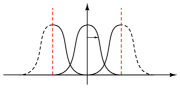
${\color[rgb]{1,0,0}-d_{\mathrm{za}}}$ ${\color[rgb]{1,0,0}+d_{\mathrm{za}}}$ $p(t)$ $0$ $\sigma$ $\Delta\omega$

Figure 5: Qualitative effect of the daily time-varying load on frequency distribution when agc is absent (p(t) denotes probability).

We simulated the system with ${D_{\mathrm{L}}=2}$, ${\mathrm{d_{za}}=100\,\mathrm{m}\mathrm{Hz}}$, i.e., with a larger dead-band, and ${P_{\mathrm{L0}}=1\,\mathrm{M}\mathrm{W}}$, thereby obtaining the \raisebox{-.9pt} {e}⃝ frequency histogram shown in Fig. 4. This new choice of dead-band is coherent with values by other tsos. Note that this large value should better contribute to keeping tgs inactive and thus to obtain a well-shaped (Gaussian) frequency histogram.

It can be noticed that no agc was introduced to compensate for the slowly varying deterministic power. As a consequence, the average frequency value varies in a slow (quasi-static) manner above and below $60\,\mathrm{Hz}$. It translates into going closer to the upper and lower limits of the dead-band. Thus, as already stated, the likelihood of crossing the dead-band and triggering the activation of tgs increases, even though ${D_{\mathrm{L}}=2}$.

We underline that the \raisebox{-.9pt} {d}⃝ and \raisebox{-.9pt} {e}⃝ histograms are obtained in two different scenarios. In the former, we have a too low (i.e., ${D_{\mathrm{L}}=0}$) load damping and, in the latter, we have a poorly managed, slowly varying power imbalance. Although the power system characteristics and setups of the two scenarios are very different, they both result in bimodal histograms.

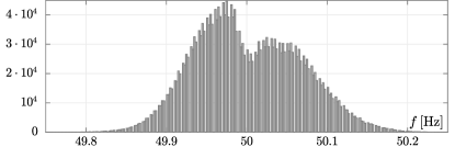
Figure 6: Frequency histogram of the Great Britain grid, June 2018. The histogram bins are uniformly distributed in the frequency interval $[49.75,50.25]\,\mathrm{Hz}$ and the bin amplitude is $2\,\mathrm{m}\mathrm{Hz}$.

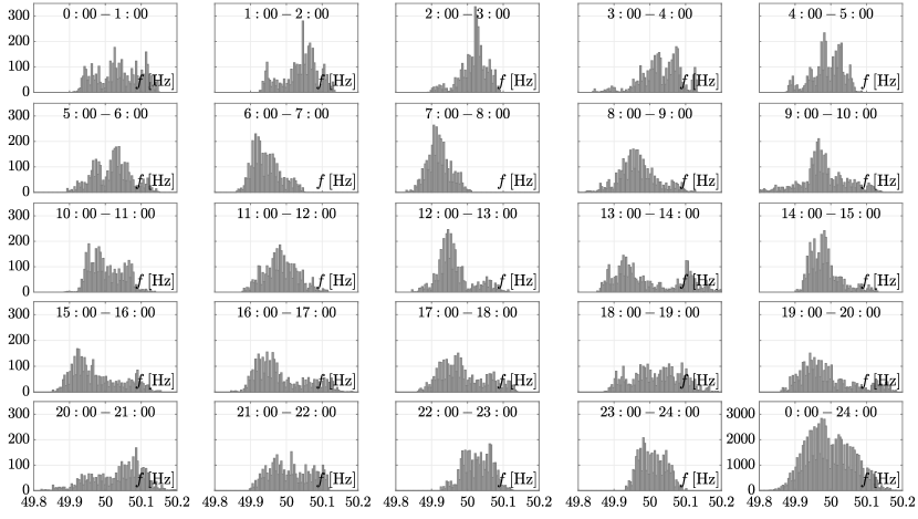
Figure 7: Frequency histograms of the Great Britain grid, June $\text{1}^{\text{st}}$, 2018. Histograms display occurrences of frequency deviations on an hourly basis. The histogram in the lower-right corner considers the samples of the entire day. The histogram bins are uniformly distributed in the frequency interval $[49.8,50.2]\,\mathrm{Hz}$ and the bin amplitude is $4\,\mathrm{m}\mathrm{Hz}$.

IV-C Bimodal frequency histograms of the Great Britain’s grid

Let us now consider a real situation, namely the frequency histogram of the Great Britain grid displayed from data recorded along with June 2018. The frequency samples are of the public domain and provided by the National Grid ESO, which is the electricity system operator for Great Britain [13]. The historic frequency data for Great Britain are provided at a $1\,\mathrm{s}$ resolution, as in our simulations. The related histogram is depicted in Fig. 6. It refers to the entire month of June. It can be seen that it has a bimodal shape. Our rhetorical question is: “Which kind of bimodal histogram is it?” Better said: “Is it of type \raisebox{-.9pt} {d}⃝ (too small $D_{\mathrm{L}}$) or \raisebox{-.9pt} {e}⃝ (inadequately handled daily power imbalance)?” The answer comes if we observe the hourly frequency histograms of the Great Britain grid for example on June $\text{1}^{\text{st}}$, 2018.

Analogous results are obtained by considering other days. Each hourly histogram seems unimodal, and none of them clearly shows any neat bimodal shape. The histograms shown in Fig. 7 highlight that there is a daily frequency drift possibly due to a mismatch of power demand and planned generation not adequately corrected by agcs and that there is some sort of dead-band. The shape of the hourly and daily histograms suggest that there may be an adequate level of load damping ($D_{\mathrm{L}}$) introduced by frequency-dependent loads.

In the monthly histogram of Fig. 6 there is an excess of occurrences due to a lack of power production with respect to power demand that leads to the asymmetry of the two peaks below and above $50\,\mathrm{Hz}$. The number of occurrences below $50\,\mathrm{Hz}$ exceeds those above. We are aware that our statements are a long shot at best since we do not have detailed information about the characteristics of the Great Britain grid. However, we dare say that monthly frequency samples aggregate may not constitute a valid indicator of the true nature (i.e., unimodal or bimodal) of power system frequency. Thus, conclusions drawn “tout court” from those could be misguided. For instance, in the case of Great Britain’s grid, a seemingly bimodal monthly frequency histogram could be due to the sum of unimodal hourly histograms collected in a power system prone to daily frequency drift.

The correct aggregation window for frequency samples depends on power system characteristics. In our scenarios, an hourly window should be adequate, since it is a time interval large enough with respect to typical power system time constants to collect a sufficient number of samples (ergodic process), but short enough compared to the slow drifting load dynamics. The same seems true for Great Britain’s case.

Another aspect worth further discussing is that the insertion of dead-bands does not limit wear and tear of tgs if the frequency drifting is not properly compensated and the frequency equilibrium point (short term average frequency) is not kept as close as possible to the nominal value.

IV-D Automatic generation control

The frequency drifting caused by the daily variation of the load/generation imbalances can be compensated by a well designed agc. In order to address this issue, we insert in the ieee 14 bus power system the simple agc model described in Section III. The transfer function of the agc is made up of a single pole in the frequency origin. Its gain has to be set so that it counteracts the hourly frequency variation caused by the deterministic drifting load, while practically filtering out the fast fluctuations due to the stochastic load.

We repeated the simulation of the scenario with the daily variable load but with narrower dead-bands. The result obtained by simulating this scenario with the $D_{\mathrm{L}}=2.0$, $\mathrm{d_{za}}=36\,\mathrm{m}\mathrm{Hz}$ and $P_{\mathrm{L0}}=1\,\mathrm{M}\mathrm{W}$ parameters is given by the \raisebox{-.9pt} {f}⃝ histogram depicted in Fig. 4. It is immediate to appreciate that the agc largely compensates for the deterministic power drift. The \raisebox{-.9pt} {f}⃝ histogram is completely different from the other two in the same figure and resembles the shape of a Gaussian probability density function that adequately lays inside the dead-band.

This result has suggested our comments on the daily histograms of the Great Britain’s grid, i.e., that there may be a poor compensation of even small power imbalances which leads to a bimodal monthly frequency histogram.

V Inertia

In presenting the frequency histograms obtained in the scenarios considered so far, we have not explicitly paid attention to the system inertia. Better said, we kept fixed the $H$ inertia parameter of all the synchronous generators and compensators of the ieee 14 bus power system. In [12] it is stated that the main factors influencing frequency distribution are the load damping and tg dead-bands, while inertia is reputed to have a minimal impact. Actually, according to (11), inertia positively influences frequency deviations, i.e., the denominator is greater than 1 and $\sigma<b$, if ${H\gg\nicefrac{{(1-2\alpha D_{\mathrm{L}}^{2})}}{{(4\alpha^{2}D_{\mathrm{L}})}}}$. We remark that if $D_{\mathrm{L}}^{2}$ is sufficiently large the right hand-side of the inequality becomes negative. It means that $H$ has a marginal role in limiting frequency deviations. Once more, we underline that $D_{\mathrm{L}}$ must assume suitable values with a proper level of $H$, otherwise the Gaussian shape of the probability density function flattens as highlighted by the simulated scenarios of Section IV. It indicates that if the inertia of a power system decreases due to higher penetration of res-fuelled converter-connected generation (and converter-connected loads), the frequency deviation can be still kept small if the value of $D_{\mathrm{L}}$ is adequately large. For example, large $D_{\mathrm{L}}$ values can be obtained by “thermostatically” controlling load such as fridges, air conditioners, and boilers [35].

To show the influence of inertia on frequency deviations, we considered three different scenarios. In each of these scenarios we have ${\mathrm{d_{za}}=36\,\mathrm{m}\mathrm{Hz}}$, ${P_{\mathrm{L0}}=1\,\mathrm{M}\mathrm{W}}$ and ${D_{\mathrm{L}}=0}$. Furthermore, we do not introduce any daily time-varying load, and thus there is no need to use agcs.

In the first and second scenarios, we multiply the $H$ inertia of each synchronous generator and compensator by ten times. Having in mind (14) and (15), in the first scenario, the simulation lasts one day, whereas in the second scenario it lasts four days. In the third scenario, we multiply by $100$ the inertia, thus remarkably increasing it and collect samples along eight days. The increase of the simulation time interval is dictated by the fact that $H^{2}$ is at the denominator in (14).

According to the common belief that inertia restoration is a must against frequency degradation, we would expect very limited frequency deviations and thus a very well shaped histogram. The three histograms corresponding to these scenarios are shown in Fig. 8.

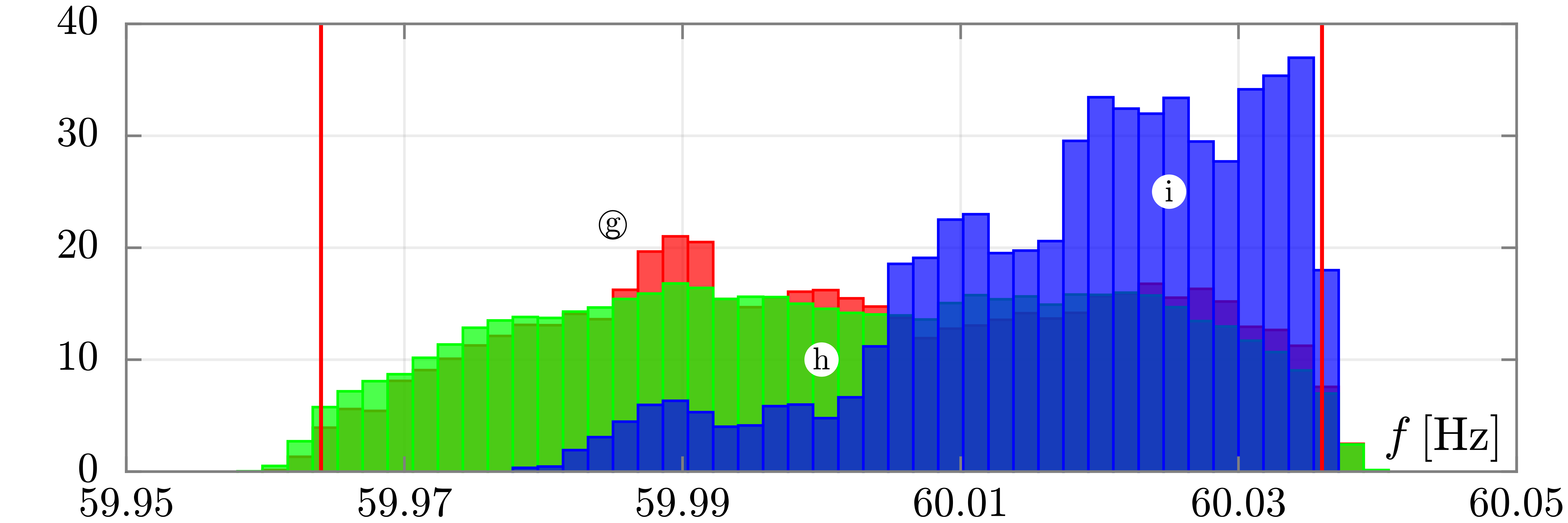
Figure 8: The \raisebox{-.9pt} {g}⃝ ($10\times H$, 1 day), \raisebox{-.9pt} {h}⃝ ($10\times H$, 4 days) and \raisebox{-.9pt} {i}⃝ ($100\times H$, 8 days) histograms correspond to the first, second and third scenarios, respectively. $\mathrm{d_{za}}=36\,\mathrm{m}\mathrm{Hz}$, $P_{\mathrm{L0}}=1\,\mathrm{M}\mathrm{W}$ $D_{\mathrm{L}}=0$. The histograms are normalised to estimate the probability density.

They are normalised to estimate the probability density and, the bins do not count occurrences as in the previous histograms. It is done since the number of samples largely differs in these three scenarios. The main aspect that we easily see is that frequency deviates from $60\,\mathrm{Hz}$ with almost the same probability inside the dead-band. When the frequency exits the dead-bands, the tgs intervene to pull the frequency back inside the dead-band. They constitute some sort of “barrier”. These histograms do not have at all the shape of a Gaussian centered at $60\,\mathrm{Hz}$, characterised by a very small variance despite the very large increase of system inertia.

We believe that this is a relevant result, which is in contrast to the common belief that inertia must be increased independently from any other aggregate parameter of a power system to counteract the negative effects of larger penetration of res generation.

VI Synthetic inertia

Most of res can be regarded as stochastic sources due to the volatility of their primary energy source (e.g., wind and sun). It means that the effects of their power output variability on frequency can be considered very similar to those of the stochastic load described in the previous sections, namely, an increase of generation can be compared to a decrease in load demand and vice versa. The main difference may be related to the statistical properties of these sources.

res can be generally considered inertia-less for two main reasons. First, as in the case of solar plants, they lack a mechanical rotating mass, which makes them incapable of exchanging and converting kinetic energy after a power mismatch to limit frequency variations. Second, unless synthetic inertia is implemented, such plants are typically connected to the grid through power electronic converters whose control schemes do not allow to modify their power output based on frequency fluctuations.

In this section, we evaluate how frequency variations can be mitigated through the installation of an aggregated photovoltaic (pv) power plant connected to the ieee 14 bus power system at bus11 through a converter implementing synthetic inertia. The word synthetic means that the converter controls are such that, when a power mismatch occurs, the behavior of the power plant in terms of power and energy exchange resembles that of a synchronous generator. It is worth noticing that synthetic inertia does an “endogenous” action by leveling the fluctuations of the res and an “exogenous” action by counterbalancing the stochastic variations of external loads.

The block schematic of the pv power plant with synthetic inertia is shown in Fig. 9.

$P_{PV}$ $I_{PV}$ $DC$ $DC$ $DC$ $AC$ $V_{PV}$ $P_{OUT}$ $V_{DC}$ $DC$ $DC$

Figure 9: Connection scheme of the pv plant and battery pack to the ieee 14 bus power system. $V_{\mathrm{pv}}^{\mathrm{ref}}=700\mathrm{V}$, $I_{\mathrm{pv}}^{\mathrm{ref}}=2.8571\mathrm{k}\mathrm{A}$, $V_{\mathrm{dc}}^{\mathrm{ref}}=680\mathrm{V}$. The superscript ^ref denotes the reference pv plant operating conditions considered during simulation.

In this design, we are only interested in the high-level behavior of the system and thus we acted with this target during its design. A pv field supplies power to the dc/dc converter that is equipped with a maximum power point tracker. The dc link voltage is kept constant by the dc/dc bidirectional converter connected to the battery pack. The power delivered/absorbed by the bidirectional dc/ac converter is set by the maximum power point tracker, by the dc/dc converter and by the specific control schema that implements synthetic inertia. An important aspect of implementing the synthetic inertia controller is the maximum power that can be delivered by the dc/ac converter and the energy capacity of the storage system. In our case, the peak power capacity of the pv field and the dc/ac converter are respectively $1$ and $2\,\mathrm{M}\mathrm{W}$, whereas the energy stored in the battery pack is ${\cal E}_{1}=160\,\mathrm{M}\mathrm{J}$ or ${\cal E}_{2}=320\,\mathrm{M}\mathrm{J}$. These design choices allow for power and energy variations comparable to those of the stochastic load. As a consequence, on average synthetic inertia does not contribute either net power or energy.

We performed simulations with the addition of synthetic inertia and with different setups. In the first case, we set $D_{\mathrm{L}}=0$, $P_{\mathrm{L0}}=1\,\mathrm{M}\mathrm{W}$ and used the ${\cal E}_{1}$ battery pack; in the second case, we used the ${\cal E}_{2}$ battery pack, and in the third case, we used ${\cal E}_{1}$ but set $D_{\mathrm{L}}=2$. In all these cases, we set $\mathrm{d_{za}}=36\,\mathrm{m}\mathrm{Hz}$ and turned off the daily time-varying load and the agc.

The results obtained in the three cases are depicted in Fig. 10. We replicated the \raisebox{-.9pt} {b}⃝ histogram of Fig. 3 in Fig. 10. These histograms can be compared to assess the significant, beneficial effect of synthetic inertia on the frequency distribution.

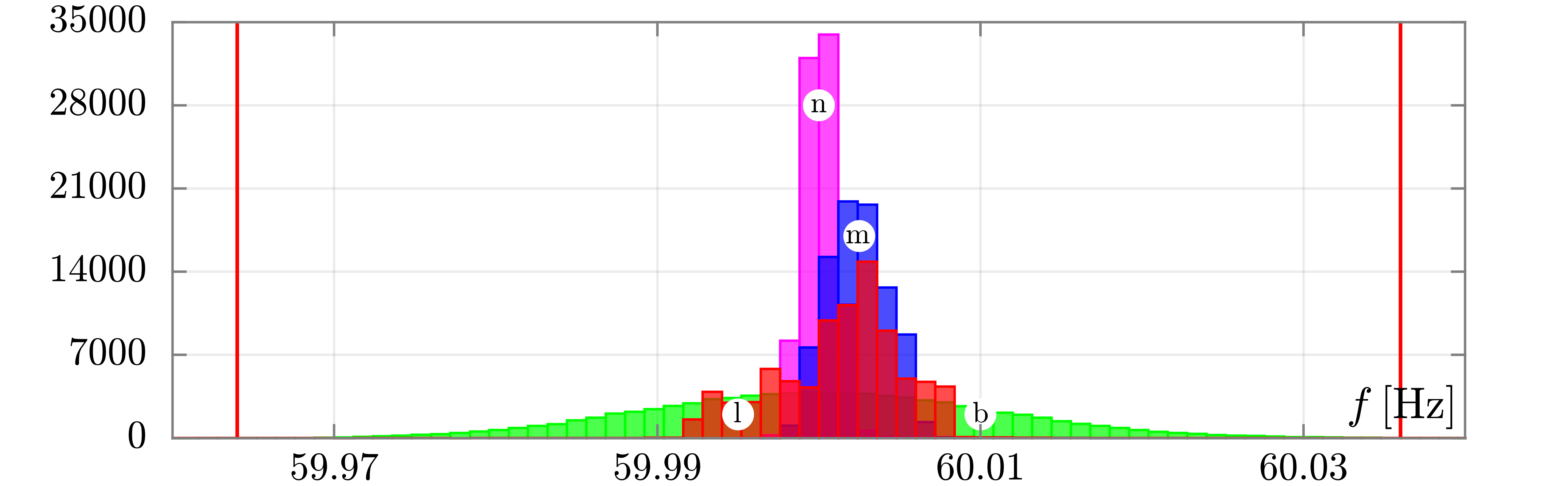
Figure 10: The frequency histograms obtained when the pv field implementing synthetic inertia is added to the ieee14 power system with no agc, no daily time-varying load, and $P_{\mathrm{L0}}=1\,\mathrm{M}\mathrm{W}$. Vertical lines correspond to the dead-band thresholds. $D_{\mathrm{L}}=0$ in the \raisebox{-.9pt} {l}⃝ (${\cal E}_{1}$ battery pack) and \raisebox{-.9pt} {m}⃝ (${\cal E}_{2}$ battery pack) histograms. $D_{\mathrm{L}}=2$ in the \raisebox{-.9pt} {n}⃝ (${\cal E}_{1}$ battery pack). The \raisebox{-.9pt} {b}⃝ histogram is the same of Fig. 3.

The histogram of Fig. 10 shows that when synthetic inertia is active almost all frequency deviations occurrences concentrate in a very small interval around $60\,\mathrm{Hz}$. It happens since the reversal time of the stochastic load is $2\,\mathrm{s}$ while the bandwidth of the controller implementing synthetic inertia is about $1\,\mathrm{k}\mathrm{Hz}$. The controller is relatively fast and efficiently manages the stochastic load by practically keeping frequency close to $60\,\mathrm{Hz}$. When we use the ${\cal E}_{2}$ battery pack, the frequency deviations are narrower than those obtained with the ${\cal E}_{1}$ battery pack. Both histograms do not have a Gaussian shape since $D_{\mathrm{L}}=0$. The interesting aspect is that when $D_{\mathrm{L}}=2$ and we use the ${\cal E}_{1}$ battery pack we obtain a well-shaped Gaussian histogram with a peak of occurrence greater than that of the \raisebox{-.9pt} {a}⃝ case of Fig. 3 that was obtained without dead-bands, i.e., with the contribution of tgs to control frequency deviations. In this case, there was not any intervention by tgs to control frequency. The need for relatively small capacity of the battery pack with respect to the very large kinetic energy stored in the full ieee 14 bus system is since it can be largely and quickly exchanged with the grid even when frequency variation is small. It does not apply to a synchronous generator since the exchanged energy is only a fraction of the stored kinetic energy due to the limited relative frequency variation. It shows that the use of synthetic inertia may be extremely convenient and viable to control frequency fluctuations due to stochastic loads [12, 36, 37].

VII Conclusion

In this paper, we focused on the reasons that lead to unwanted frequency distributions, such as bimodal ones. We presented both analytical and numerical results. The former derive from the rigorous analysis of a simplified and linear power system model and allowed us to highlight some important focal points.

• The smaller the load damping coefficient, the lower the effectiveness of inertia in limiting frequency deviations. This is in contrast to the common idea that an increment of the overall system inertia is beneficial, regardless of the value of other aggregate system parameters.

• The load damping coefficient is deemed to play a significant role in limiting frequency variations and it could be increased by exploiting for example thermostatically controlled loads that link frequency variations to the absorbed power, as well as load damping and synthetic inertia, which require a suitable implementation of res generation and storage systems.

• The reduction of the load damping coefficient leads to an increased probability of crossing the dead-bands implemented in tgs and, thus, of obtaining bimodal frequency histograms.

According to the numerical results that we derived through a set of simulations of the well-known ieee 14 bus power system, we draw the following conclusions.

• Inertia together with turbine controls plays a significant role to contain large frequency deviations and thus to keep operational security, when severe contingencies happen in a power grid. However, in case of small stochastic fluctuations of load/generation, an increase, even extremely large, of system inertia does not lead to a Gaussian frequency distribution if the load damping does not have a proper value. This means that to have small and well-shaped frequency variations we have to simultaneously act on these two system parameters.

• Any slow deterministic frequency drift, albeit small, must be compensated to avoid tear and wear of tgs when dead-bands are implemented. For example, this has to be accomplished by well-designed agcs. Acting on electronic controllers of load and res is beneficial if they both increase inertia (synthetic) and load damping (synthetic).

These considerations have general validity since our analysis considered the ieee 14 bus power system as one among several ones. We could have chosen other known power system models to draw the same conclusions above (as we did to test results). The reported histograms of frequency deviations constitute a logic “path” through which the reader is conducted to the considerations we draw. In the light of the conclusions, a real situation, namely the frequency histogram of the Great Britain grid displayed from data recorded along with June 2018, was analyzed. It led us also to some considerations concerning the definition of a correct aggregation procedure to deal with historic frequency data.

References

- [1] P. Kundur, Power system stability and control. New York: McGraw-Hill, 1994.
- [2] North American Electric Reliability Corporation (NERC), Balancing and Frequency Control, 2011.
- [3] ——, Frequency Response Initiative Report: The Reliability Role of Frequency Response, 2012.
- [4] B. Kroposki, B. Johnson, Y. Zhang, V. Gevorgian, P. Denholm, B. . Hodge, and B. Hannegan, “Achieving a 100% renewable grid: Operating electric power systems with extremely high levels of variable renewable energy,” IEEE Power Energy Mag., vol. 15, no. 2, pp. 61–73, 2017.
- [5] F. Arrigo, E. Bompard, M. Merlo, and F. Milano, “Assessment of primary frequency control through battery energy storage systems,” Int. J. Electr. Power Energy Syst., vol. 115, p. 105428, 2020.
- [6] Z. A. Obaid, L. M. Cipcigan, L. Abrahim, and M. T. Muhssin, “Frequency control of future power systems: reviewing and evaluating challenges and new control methods,” J. Mod. Power Syst. Clean Energy, vol. 7, no. 1, pp. 9–25, 2019.
- [7] A. Ulbig, T. S. Borsche, and G. Andersson, “Impact of low rotational inertia on power system stability and operation,” in IFAC Proceedings Volumes (IFAC-PapersOnline), vol. 19, 2014, pp. 7290–7297.
- [8] P. Tielens and D. Van Hertem, “The relevance of inertia in power systems,” Renew. Sust. Energ. Rev., vol. 55, pp. 999–1009, 2016.
- [9] U. Tamrakar, D. Shrestha, M. Maharjan, B. P. Bhattarai, T. M. Hansen, and R. Tonkoski, “Virtual inertia: Current trends and future directions,” Applied Sciences (Switzerland), vol. 7, no. 7, 2017.
- [10] North American Electric Reliability Corporation (NERC), 2019 Frequency Response Annual Analysis, 2019.
- [11] F. M. Mele, A. Ortega, R. Zarate-Minano, and F. Milano, “Impact of variability, uncertainty and frequency regulation on power system frequency distribution,” in Power Systems Computation Conference (PSCC), Jun. 2016, pp. 1–8.
- [12] P. Vorobev, D. M. Greenwood, J. H. Bell, J. W. Bialek, P. C. Taylor, and K. Turitsyn, “Deadbands, droop, and inertia impact on power system frequency distribution,” IEEE Trans. Power Syst., vol. 34, no. 4, pp. 3098–3108, Jul. 2019.
-
[13]
National grid frequency data for 2016,
https://www.nationalgrideso.com/
balancing-services/frequency-response-services/historic-frequency-data. - [14] F. Milano and R. Zárate-Miñano, “A systematic method to model power systems as stochastic differential algebraic equations,” IEEE Trans. Power Syst., vol. 28, no. 4, pp. 4537–4544, Nov. 2013.
- [15] R. Singh, B. C. Pal, and R. A. Jabr, “Statistical representation of distribution system loads using gaussian mixture model,” IEEE Trans. Power Syst., vol. 25, no. 1, pp. 29–37, Feb. 2010.
- [16] A. K. Ghosh, D. L. Lubkeman, M. J. Downey, and R. H. Jones, “Distribution circuit state estimation using a probabilistic approach,” IEEE Trans. Power Syst., vol. 12, no. 1, pp. 45–51, 1997.
- [17] C. Delgado and J. Domínguez-Navarro, “Point estimate method for probabilistic load flow of an unbalanced power distribution system with correlated wind and solar sources,” Int. J. Electr. Power Energy Syst., vol. 61, pp. 267–278, 2014.
- [18] L. Arnold, Stochastic Differential Equations: Theory and Applications. Wiley, 1974.
- [19] D. T. Gillespie, “Exact numerical simulation of the ornstein-uhlenbeck process and its integral,” Phys. Rev. E, vol. 54, pp. 2084–2091, Aug. 1996. [Online]. Available: https://link.aps.org/doi/10.1103/PhysRevE.54.2084
- [20] H. Zhao, Q. Wu, S. Huang, H. Zhang, Y. Liu, and Y. Xue, “Hierarchical control of thermostatically controlled loads for primary frequency support,” IEEE Trans. Smart Grid, vol. 9, no. 4, pp. 2986–2998, Jul. 2018.
- [21] Z. Xu, J. Ostergaard, M. Togeby, and C. Marcus-Moller, “Design and modelling of thermostatically controlled loads as frequency controlled reserve,” in Procs. of the IEEE PES General Meeting, June 2007, pp. 1–6.
- [22] H. Hao, B. M. Sanandaji, K. Poolla, and T. L. Vincent, “Aggregate flexibility of thermostatically controlled loads,” IEEE Trans. Power Syst., vol. 30, no. 1, pp. 189–198, Jan. 2015.
- [23] F. Baccino, F. Conte, S. Massucco, F. Silvestro, and S. Grillo, “Frequency Regulation by Management of Building Cooling Systems Through Model Predictive Control,” in 2014 Power Systems Computation Conference (PSCC), 2014, pp. 1–7.
- [24] V. Trovato, I. M. Sanz, B. Chaudhuri, and G. Strbac, “Advanced control of thermostatic loads for rapid frequency response in great britain,” IEEE Trans. Power Syst., vol. 32, no. 3, pp. 2106–2117, May 2017.
- [25] F. Jibji-Bukar and O. Anaya-Lara, “Frequency support from photovoltaic power plants using offline maximum power point tracking and variable droop control,” IET Renewable Power Generation, 2019.
- [26] J. Fang, P. Lin, H. Li, Y. Yang, and Y. Tang, “An improved virtual inertia control for three-phase voltage source converters connected to a weak grid,” IEEE Trans. Power Electron., vol. 34, pp. 8660–8670, Sep. 2019.
- [27] J. Kim, V. Gevorgian, Y. Luo, M. Mohanpurkar, V. Koritarov, R. Hovsapian, and E. Muljadi, “Supercapacitor to provide ancillary services with control coordination,” IEEE Trans. Ind. Appl., vol. 55, no. 5, pp. 5119–5127, 2019.
- [28] F. Bizzarri and A. Brambilla, “PAN and MPanSuite: Simulation vehicles towards the analysis and design of heterogeneous mixed electrical systems,” in IEEE International Conference of New Generation of Circuits and Systems (NGCAS), Sep. 2017, pp. 1–4.
- [29] F. Milano, Power System Modelling and Scripting. London: Springer, 2010.
- [30] ——, “A Python-based software tool for power system analysis,” in Procs. of the IEEE PES General Meeting, Vancouver, BC, Jul. 2013.
- [31] M. Liu, F. Bizzarri, A. M. Brambilla, and F. Milano, “On the impact of the dead-band of power system stabilizers and frequency regulation on power system stability,” IEEE Trans. Power Syst., vol. 34, no. 5, pp. 3977–3979, Sep. 2019.
- [32] Y. Zhang, W. Yao, S. You, W. Yu, L. Wu, Y. Cui, and Y. Liu, “Impacts of power grid frequency deviation on time error of synchronous electric clock and worldwide power system practices on time error correction,” Energies, vol. 10, pp. 1–15, 08 2017.
- [33] P. M. Ashton, C. S. Saunders, G. A. Taylor, A. M. Carter, and M. E. Bradley, “Inertia estimation of the gb power system using synchrophasor measurements,” IEEE Trans. Power Syst., vol. 30, no. 2, pp. 701–709, Mar. 2015.
- [34] R. Hollinger, A. M. Cortes, and T. Erge, “Fast frequency response with bess: A comparative analysis of germany, great britain and sweden,” in 15th International Conference on the European Energy Market (EEM), Jun. 2018, pp. 1–6.
- [35] F. Conte, S. Massucco, F. Silvestro, E. Ciapessoni, and D. Cirio, “Stochastic modelling of aggregated thermal loads for impact analysis of demand side frequency regulation in the case of sardinia in 2020,” Int. J. Electr. Power Energy Syst., vol. 93, pp. 291–307, 2017.
- [36] Z. X. Tang, Y. S. Lim, S. Morris, J. L. Yi, P. F. Lyons, and P. C. Taylor, “A comprehensive work package for energy storage systems as a means of frequency regulation with increased penetration of photovoltaic systems,” Int. J. Electr. Power Energy Syst., vol. 110, pp. 197–207, 2019.
- [37] G. Magdy, G. Shabib, A. A. Elbaset, and Y. Mitani, “Renewable power systems dynamic security using a new coordination of frequency control strategy based on virtual synchronous generator and digital frequency protection,” Int. J. Electr. Power Energy Syst., vol. 109, pp. 351–368, 2019.