Switching problems with controlled randomisation and associated obliquely reflected BSDEs

Abstract

We introduce and study a new class of optimal switching problems, namely switching problem with controlled randomisation, where some extra-randomness impacts the choice of switching modes and associated costs. We show that the optimal value of the switching problem is related to a new class of multidimensional obliquely reflected BSDEs. These BSDEs allow as well to construct an optimal strategy and thus to solve completely the initial problem. The other main contribution of our work is to prove new existence and uniqueness results for these obliquely reflected BSDEs. This is achieved by a careful study of the domain of reflection and the construction of an appropriate oblique reflection operator in order to invoke results from [7].

1 Introduction

In this work, we introduce and study a new class of optimal switching problems in stochastic control theory. The interest in switching problems comes mainly from their connections to financial and economic problems, like the pricing of real options [4]. In a celebrated article [14], Hamadène and Jeanblanc study the fair valuation of a company producing electricity. In their work, the company management can choose between two modes of production for their power plant –operating or close– and a time of switching from one state to another, in order to maximise its expected return. Typically, the company will buy electricity on the market if the power station is not operating. The company receives a profit for delivering electricity in each regime. The main point here is that a fixed cost penalizes the profit upon switching. This switching problem has been generalized to more than two modes of production [10]. Let us now discuss this switching problem with $d\geq 2$ modes in more details. The costs to switch from one state to another are given by a matrix $(c_{i,j})_{1\leq i,j\leq d}$. The management optimises the expected company profits by choosing switching strategies which are sequences of stopping times $(\tau_{n})_{n\geq 0}$ and modes $(\zeta_{n})_{n\geq 0}$. The current state of the strategy is given by $a_{t}=\sum_{k=0}^{+\infty}\zeta_{k}1_{[\tau_{k},\tau_{k+1})}(t),\;t\in[0,T]\;,$ where $T$ is a terminal time. To formalise the problem, we assume that we are working on a complete probability space $(\Omega,\mathcal{A},\mathbb{P})$ supporting a Brownian Motion $W$. The stopping times are defined with respect to the filtration $(\mathcal{F}_{t})_{t\geq 0}$ generated by this Brownian motion. Denoting by $f(t,i)$ the instantaneous profit received at time $t$ in mode $i$, the time cumulated profit associated to a switching strategy is given by $\int_{0}^{T}f(t,a_{t})\mathrm{d}t-\sum_{k=0}^{+\infty}c_{\zeta_{k},\zeta_{k+1}}1_{\left\{\tau_{k+1}\leq t\wedge T\right\}}$. The management solves then at the initial time the following control problem

$$\mathcal{V}_{0}=\sup_{a\in\mathscr{A}}\mathbb{E}\!\!\left[\int_{0}^{T}f(t,a_{t})\mathrm{d}t-\sum_{k=0}^{+\infty}c_{\zeta_{k},\zeta_{k+1}}1_{\left\{\tau_{k+1}\leq T\right\}}\right]\,,$$ (1.1)

where $\mathscr{A}$ is a set of admissible strategies that will be precisely described below (see Section 2.1). We shall refer to problems of the form (1.1) under the name of classical switching problems. These problems have received a lot of interest and are now quite well understood [14, 10, 17, 5]. In our work, we introduce a new kind of switching problem, to model more realistic situations, by taking into account uncertainties that are encountered in practice. Coming back to the simple but enlightning example of an electricity producer described in [14], we introduce some extra-randomness in the production process. Namely, when switching to the operating mode, it may happen with –hopefully– a small probability that the station will have some dysfunction. This can be represented by a new mode of “production” with a greater switching cost than the business as usual one. To capture this phenomenon in our mathematical model, we introduce a randomisation procedure: the management decides the time of switching but the mode is chosen randomly according to some extra noise source. We shall refer to this kind of problem by randomised switching problem. However, we do not limit our study to this framework. Indeed, we allow some control by the agent on this randomisation. Namely, the agent can chose optimally a probability distributions $P^{u}$ on the modes space given some parameter $u\in\mathcal{C}$, in the control space. The new mode $\zeta_{k+1}$ is then drawn, independently of everything up to now, according to this distribution $P^{u}$ and a specific switching cost $c^{u}_{\zeta_{k},\zeta_{k+1}}$ is applied. The management strategy is thus given now by the sequence $(\tau_{k},u_{k})_{k\geq 0}$ of switching times and controls. The maximisation problem is still given by (1.1). Let us observe however that $\mathbb{E}\!\!\left[c^{u_{k}}_{\zeta_{k},\zeta_{k+1}}\right]=\mathbb{E}\!\!\left[\sum_{1\leqslant j\leqslant d}P^{u_{k}}_{\zeta_{k},j}c^{u_{k}}_{\zeta_{k},j}\right]$, thanks to the tower property of conditional expectation. In particular, we will only work with the mean switching costs $\bar{c}^{u_{k}}_{i}:=\sum_{1\leqslant j\leqslant d}P^{u_{k}}_{i,j}c^{u_{k}}_{i,j}$ in (1.1). We name this kind of control problem switching problem with controlled randomisation. Although their apparent modeling power, this kind of control problem has not been considered in the literature before, to the best of our knowledge. In particular, we will show that the classical or randomised switching problem are just special instances of this more generic problem. The switching problem with controlled randomisation is introduced rigorously in Section 2.1 below.

A key point in our work is to relate the control problem under consideration to a new class of obliquely reflected Backward Stochastic Differential Equations (BSDEs). In the first part, following the approach of [14, 10, 17], we completely solve the switching problem with controlled randomisation by providing an optimal strategy. The optimal strategy is built by using the solution to a well chosen obliquely reflected BSDE. Although this approach is not new, the link between the obliquely reflected BSDE and the switching problem is more subtle than in the classical case due to the state uncertainty. In particular, some care must be taken when defining the adaptedness property of the strategy and associated quantities. Indeed, a tailor-made filtration, studied in details in Appendix A.2, is associated to each admissible strategy. The state and cumulative cost processes are adapted to this filtration, and the associated reward process is defined as the $Y$-component of the solution to some “switched” BSDE in this filtration. The classical estimates used to identify an optimal strategy have to be adapted to take into account the extra orthogonal martingale arising when solving this “switched” BSDE in a non Brownian filtration.

In the second part of our work, we study the auxiliary obliquely reflected BSDE, which is written in the Brownian filtration and represents the optimal value in all the possible starting modes. Reflected BSDEs were first considered by Gegout-Petit and Pardoux [13], in a multidimensional setting of normal reflections. In one dimension, they have also been studied in [11] in the so called simply reflected case, and in [8] in the doubly reflected case. The multidimensional RBSDE associated to the classical switching problem is reflected in a specific convex domain and involves oblique directions of reflection. Due to the controlled randomisation, the domain in which the $Y$-component of the auxiliary RBSDE is constrained is different from the classical switching problem domain and its shape varies a lot from one model specification to another. The existence of a solution to the obliquely reflected BSDE has thus to be studied carefully. We do so by relying on the article [7], that studies, in a generic way, the obliquely reflected BSDE in a fixed convex domain in both Markovian and non-Markovian setting. The main step for us here is to exhibit an oblique reflection operator, with the good properties to use the results in [7]. We are able to obtain new existence results for this class of obliquely reflected BSDEs. Because we are primarily interested in solving the control problem, we derive the uniqueness of the obliquely reflected BSDEs in the Hu and Tang specification for the driver [17], namely $f^{i}(t,y,z):=f^{i}(t,y^{i},z^{i})$ for $i\in\{1,\dots,d\}$. But our results can be easily generalized to the specification $f^{i}(t,y,z):=f^{i}(t,y,z^{i})$ by using similar arguments as in [6].

The rest of the paper is organised as follows. In Section 2, we introduce the switching problem with controlled randomisation. We prove that, if there exists a solution to the associated BSDE with oblique reflections, then its $Y$-component coincides with the value of the switching problem. A verification argument allows then to deduce uniqueness of the solution of the obliquely reflected BSDE. In Section 3, we show that there exists indeed a solution to the obliquely reflected BSDE under some conditions on the parameters of the switching problem and its randomisation. We also prove uniqueness of the solution under some structural condition on the driver $f$. Finally, we gather in the Appendix section some technical results.

Notations

If $n\geq 1$, we let $\mathcal{B}^{n}$ be the Borelian sigma-algebra on $\mathbb{R}^{n}$.
For any filtered probability space $(\Omega,\mathcal{G},\mathbb{F},\mathbb{P})$ and constants $T>0$ and $p\geq 1$, we define the following spaces:

• $L^{p}_{n}(\mathcal{G})$ is the set of $\mathcal{G}$-measurable random variables $X$ valued in $\mathbb{R}^{n}$ satisfying $\mathbb{E}\!\!\left[|X|^{p}\right]<+\infty$,

• $\mathcal{P}(\mathbb{F})$ is the predictable sigma-algebra on $\Omega\times[0,T]$,

• $\mathbb{H}^{p}_{n}(\mathbb{F})$ is the set of predictable processes $\phi$ valued in $\mathbb{R}^{n}$ such that

  $$\mathbb{E}\!\!\left[\int_{0}^{T}|\phi_{t}|^{p}\mathrm{d}t\right]<+\infty,$$ (1.2)

• $\mathbb{S}^{p}_{n}(\mathbb{F})$ is the set of càdlàg processes $\phi$ valued in $\mathbb{R}^{n}$ such that

  $$\mathbb{E}\!\!\left[\sup_{0\leq t\leq T}|\phi_{t}|^{p}\right]<+\infty,$$ (1.3)

• $\mathbb{A}^{p}_{n}(\mathbb{F})$ is the set of continuous processes $\phi$ valued in $\mathbb{R}^{n}$ such that $\phi_{T}\in L^{p}_{n}(\mathcal{F}_{T})$ and $\phi^{i}$ is nondecreasing for all $i=1,\dots,n$.

If $n=1$, we omit the subscript $n$ in previous notations.
For $d\geq 1$, we denote by $(e_{i})_{i=1}^{d}$ the canonical basis of $\mathbb{R}^{d}$ and $S_{d}(\mathbb{R})$ the set of symmetric matrices of size $d\times d$ with real coefficients.
If $\mathcal{D}$ is a convex subset of $\mathbb{R}^{d}$ ($d\geq 1$) and $y\in\mathcal{D}$, we denote by $\mathcal{C}(y)$ the outward normal cone at $y$, defined by

$$\mathcal{C}(y):=\{v\in\mathbb{R}^{d}:v^{\top}(z-y)\leq 0\mbox{ for all }z\in\mathcal{D}\}.$$ (1.4)

We also set $\mathfrak{n}(y):=\mathcal{C}(y)\cap\{v\in\mathbb{R}^{d}:|v|=1\}$.
If $X$ is a matrix of size $n\times m$, $\mathcal{I}\subset\{1,\dots,n\}$ and $\mathcal{J}\subset\{1,\dots,m\}$, we set $X^{(\mathcal{I},\mathcal{J})}$ the matrix of size $(n-|\mathcal{I}|)\times(m-|\mathcal{J}|)$ obtained from $X$ by deleting rows with index $i\in\mathcal{I}$ and columns with index $j\in\mathcal{J}$. If $\mathcal{I}=\{i\}$ we set $X^{(i,\mathcal{J})}:=X^{(\mathcal{I},\mathcal{J})}$, and similarly if $\mathcal{J}=\{j\}$.
If $v$ is a vector of size $n$ and $1\leq i\leq n$, we set $v^{(i)}$ the vector of size $n-1$ obtained from $v$ by deleting coefficient $i$.

For $(i,j)\in\{1,\dots,d\}$, we define $i^{(j)}:=i-{\bf 1}_{\{i>j\}}\in\{1,\dots,d-1\}\;$, for $d\geq 2$.
We denote by $\succcurlyeq$ the component by component partial ordering relation on vectors and matrices.

2 Switching problem with controlled randomisation

We introduce here a new kind of stochastic control problem that we name switching problem with controlled randomisation. In contrast with the usual switching problems [14, 16, 17], the agent cannot choose directly the new state, but chooses a probability distribution under which the new state will be determined. In this section, we assume the existence of a solution to some auxiliary obliquely reflected BSDE to characterize the value process and an optimal strategy for the problem, see Assumption 2.2 below.

Let $(\Omega,\mathcal{G},\mathbb{P})$ be a probability space. We fix a finite time horizon $T>0$ and $\kappa\geq 1,d\geq 2$ two integers. We assume that there exists a $\kappa$-dimensional Brownian motion $W$ and a sequence $(\mathfrak{U}_{n})_{n\geq 1}$ of independent random variables, independent of $W$, uniformly distributed on $[0,1]$. We also assume that $\mathcal{G}$ is generated by the Brownian motion $W$ and the family $(\mathfrak{U}_{n})_{n\geq 1}$. We define $\mathbb{F}^{0}=(\mathcal{F}^{0}_{t})_{t\geq 0}$ as the augmented Brownian filtration, which satisfies the usual conditions.
Let $\mathcal{C}$ be an ordered compact metric space and $F:\mathcal{C}\times\{1,\dots,d\}\times[0,1]\to\{1,\dots,d\}$ a measurable map. To each $u\in\mathcal{C}$ is associated a transition probability function on the state space $\{1,\dots,d\}$, given by $P^{u}_{i,j}:=\mathbb{P}(F(u,i,\mathfrak{U})=j)$ for $\mathfrak{U}$ uniformly distributed on $[0,1]$. We assume that for all $(i,j)\in\{1,\dots,d\}^{2}$, the map $u\mapsto P^{u}_{i,j}$ is continuous.
Let $\bar{c}:\{1,\dots,d\}\times\mathcal{C}\to\mathbb{R}_{+},(i,u)\mapsto\bar{c}_{i}^{u}$ a map such that $u\mapsto\bar{c}^{u}_{i}$ is continuous for all $i=1,\dots,d$. We denote $\sup_{i\in\{1,\dots,d\},u\in\mathcal{C}}\bar{c}_{i}^{u}:=\check{c}$ and $\inf_{i\in\{1,\dots,d\},u\in\mathcal{C}}\bar{c}_{i}^{u}:=\hat{c}$.
Let $\xi=(\xi^{1},\dots,\xi^{d})\in L^{2}_{d}(\mathcal{F}^{0}_{T})$ and $f:\Omega\times[0,T]\times\mathbb{R}^{d}\times\mathbb{R}^{d\times\kappa}\to\mathbb{R}^{d}$ a map satisfying

• $f$ is $\mathcal{P}(\mathbb{F}^{0})\otimes\mathcal{B}^{d}\otimes\mathcal{B}^{d\times\kappa}$-measurable and $f(\cdot,0,0)\in\mathbb{H}^{2}_{d}(\mathbb{F}^{0})$.

• There exists $L\geq 0$ such that, for all $(t,y,y^{\prime},z,z^{\prime})\in[0,T]\times\mathbb{R}^{d}\times\mathbb{R}^{d}\times\mathbb{R}^{d\times\kappa}\times\mathbb{R}^{d\times\kappa}$,

  $$|f(t,y,z)-f(t,y^{\prime},z^{\prime})|\leq L(|y-y^{\prime}|+|z-z^{\prime}|).$$

These assumptions will be in force throughout our work. We shall also use, in this section only, the following additional assumptions.

Assumption 2.1.

1. Switching costs are assumed to be positive, i.e. $\hat{c}>0$.

2. For all $(t,y,z)\in[0,T]\times\mathbb{R}^{d}\times\mathbb{R}^{d\times\kappa}$, it holds almost surely,

   $$f(t,y,z)=(f^{i}(t,y^{i},z^{i}))_{1\leq i\leq d}.$$ (2.1)

Remark 2.1.

i) It is usual to assume positive costs in the litterature on switching problem. In particular, the cumulative cost process, see (2.2), is non decreasing. Introducing signed costs adds extra technical difficulties in the proof of the representation theorem (see e.g. [19] and references therein). We postpone the adaptation of our results in this more general framework to future works.
ii) Assumption (2.1) is also classical since it allows to get a comparison result for BSDEs which is key to obtain the representation theorem. Note however than our results can be generalized to the case $f^{i}(t,y,z)=f^{i}(t,y,z^{i})$ for $i\in\{1,...,d\}$ by using similar arguments as in [5].

2.1 Solving the control problem using obliquely reflected BSDEs

We define in this section the stochastic optimal control problem. We first introduce the strategies available to the agent and related processes. The definition of the strategy is more involved than in the usual switching problem setting since its adaptiveness property is understood with respect to a filtration built recursively.

A strategy is thus given by $\phi=\left(\zeta_{0},(\tau_{n})_{n\geq 0},(\alpha_{n})_{n\geq 1}\right)$ where $\zeta_{0}\in\{1,\dots,d\}$, $(\tau_{n})_{n\geq 0}$ is a nondecreasing sequence of random times and $(\alpha_{n})_{n\geq 1}$ is a sequence of $\mathcal{C}$-valued random variables, which satisfy:

• $\tau_{0}\in[0,T]$ and $\zeta_{0}\in\{1,\dots,d\}$ are deterministic.

• For all $n\geq 0$, $\tau_{n+1}$ is a $\mathbb{F}^{n}$-stopping time and $\alpha_{n+1}$ is $\mathcal{F}^{n}_{\tau_{n+1}}$-measurable (recall that $\mathbb{F}^{0}$ is the augmented Brownian filtration). We then set $\mathbb{F}^{n+1}=(\mathcal{F}^{n+1}_{t})_{t\geq 0}$ with $\mathcal{F}^{n+1}_{t}:=\mathcal{F}^{n}_{t}\vee\sigma(\mathfrak{U}_{n+1}1_{\left\{\tau_{n+1}\leq t\right\}})$.

Lastly, we define $\mathbb{F}^{\infty}=(\mathcal{F}^{\infty}_{t})_{t\geq 0}$ with $\mathcal{F}^{\infty}_{t}:=\bigvee_{n\geq 0}\mathcal{F}^{n}_{t},t\geq 0$.
For a strategy $\phi=\left(\zeta_{0},(\tau_{n})_{n\geq 0},(\alpha_{n})_{n\geq 1}\right)$, we set, for $n\geq 0$,

$$\zeta_{n+1}:=F(\alpha_{n+1},\zeta_{n},\mathfrak{U}_{n+1})\text{ and }a_{t}:=\sum_{k=0}^{+\infty}\zeta_{k}1_{[\tau_{k},\tau_{k+1})}(t),\;t\geq 0\;,$$

which represents the state after a switch and the state process respectively. We also introduce two processes, for $t\geq 0$,

$$A^{\phi}_{t}=\sum_{k=0}^{+\infty}\bar{c}_{\zeta_{k}}^{\alpha_{k+1}}1_{\left\{\tau_{k+1}\leq t\right\}}\text{ and }N^{\phi}_{t}:=\sum_{k\geq 0}1_{\left\{\tau_{k+1}\leq t\right\}}.$$ (2.2)

The random variable $A^{\phi}_{t}$ is the cumulative cost up to time $t$ and $N^{\phi}_{t}$ is the number of switches before time $t$. Notice that the processes $(a,A^{\phi},N^{\phi})$ are adapted to $\mathbb{F}^{\infty}$ and that $A^{\phi}$ is a non decreasing process.

We say that a strategy $\phi=(\zeta_{0},(\tau_{n})_{n\geq 0},(\alpha_{n})_{n\geq 1})$ is an admissible strategy if the cumulative cost process satisfies

$$A^{\phi}_{T}-A^{\phi}_{\tau_{0}}\in L^{2}(\mathbb{F}^{\infty}_{T})\quad\text{ and }\quad\mathbb{E}\!\!\left[\left.\left(A^{\phi}_{\tau_{0}}\right)^{2}\right|\mathcal{F}^{0}_{\tau_{0}}\right]<+\infty\;a.s.$$ (2.3)

We denote by $\mathscr{A}$ the set of admissible strategies, and for $t\in[0,T]$ and $i\in\{1,\dots,d\}$, we denote by $\mathscr{A}^{i}_{t}$ the subset of admissible strategies satisfying $\zeta_{0}=i$ and $\tau_{0}=t$.

Remark 2.2.

1. The definition of an admissible strategy is slightly weaker than usual [17], which requires the stronger property $A^{\phi}_{T}\in L^{2}(\mathcal{F}^{\infty}_{T})$. But, importantly, the above definition is enough to define the switched BSDE associated to an admissible control, see below. Moreover, we observe in the next section that optimal strategies are admissible with respect to our definition, but not necessarily with the usual one, due to possible simultaneous jumps at the initial time.

2. For technical reasons involving possible simultaneous jumps, we cannot consider the generated filtration associated to $a$, which is contained in $\mathbb{F}^{\infty}$.

We are now in position to introduce the reward associated to an admissible strategy. If $\phi=(\zeta_{0},(\tau_{n})_{n\geq 0},(\alpha_{n})_{n\geq 1})\in\mathscr{A}$, the reward is defined as the value $\mathbb{E}\!\!\left[\left.U^{\phi}_{\tau_{0}}-A^{\phi}_{\tau_{0}}\right|\mathcal{F}^{0}_{\tau_{0}}\right]$, where $(U^{\phi},V^{\phi},M^{\phi})\in\mathbb{S}^{2}(\mathbb{F}^{\infty})\times\mathbb{H}^{2}_{\kappa}(\mathbb{F}^{\infty})\times\mathbb{H}^{2}(\mathbb{F}^{\infty})$ is the solution of the following “switched” BSDE [17] on the filtered probability space $(\Omega,\mathcal{G},\mathbb{F}^{\infty},\mathbb{P})$:

$$U_{t}=\xi^{a_{T}}+\int_{t}^{T}f^{a_{s}}(s,U_{s},V_{s})\mathrm{d}s-\int_{t}^{T}V_{s}\mathrm{d}W_{s}-\int_{t}^{T}\mathrm{d}M_{s}-\int_{t}^{T}\mathrm{d}A^{\phi}_{s},\quad t\in[\tau_{0},T].$$ (2.4)

Remark 2.3.

This switched BSDE rewrites as a classical BSDE in $\mathbb{F}^{\infty}$, and since $A^{\phi}_{\cdot}-A^{\phi}_{t}\in\mathbb{S}^{2}(\mathbb{F}^{\infty})$, the terminal condition and the driver are standard parameters, there exists a unique solution to (2.4) for all $\phi\in\mathscr{A}$. We refer to Section A.2.2 for more details.

For $t\in[0,T]$ and $i\in\{1,\dots,d\}$, the agent aims thus to solve the following maximisation problem:

$$\mathcal{V}^{i}_{t}=\operatorname*{ess\,sup}_{\phi\in\mathscr{A}^{i}_{t}}\mathbb{E}\!\!\left[\left.U^{\phi}_{t}-A^{\phi}_{t}\right|\mathcal{F}^{0}_{t}\right].$$ (2.5)

We first remark that this control problem corresponds to (1.1) as soon as $f$ does not depend on $y$ and $z$. Moreover, the term $\mathbb{E}\!\!\left[\left.A^{\phi}_{t}\right|\mathcal{F}^{0}_{t}\right]$ is non zero if and only if we have at least one instantaneous switch at initial time $t$.

The main result of this section is the next theorem that relates the value process $\mathcal{V}$ to the solution of an obliquely reflected BSDEs, that is introduced in the following assumption:

Assumption 2.2.

1. There exists a solution $(Y,Z,K)\in\mathbb{S}^{2}_{d}(\mathbb{F}^{0})\times\mathbb{H}^{2}_{d\times\kappa}(\mathbb{F}^{0})\times\mathbb{A}^{2}_{d}(\mathbb{F}^{0})$ to the following obliquely reflected BSDE:

   $$Y^{i}_{t} =\xi+\int_{t}^{T}f^{i}(s,Y^{i}_{s},Z^{i}_{s})\mathrm{d}s-\int_{t}^{T}Z^{i}_{s}\mathrm{d}W_{s}+\int_{t}^{T}\mathrm{d}K^{i}_{s},\quad t\in[0,T],\,i\in\mathcal{I},$$ (2.6)

   $$Y_{t} \in\mathcal{D},\quad t\in[0,T],$$ (2.7)

   $$\int_{0}^{T} \left(Y^{i}_{t}-\sup_{u\in\mathcal{C}}\left\{\sum_{j=1}^{d}P^{u}_{i,j}Y^{j}_{t}-\bar{c}_{i}^{u}\right\}\right)\mathrm{d}K^{i}_{t}=0,\quad i\in\mathcal{I},$$ (2.8)

   where $\mathcal{I}:=\{1,\dots,d\}$ and $\mathcal{D}$ is the following convex subset of $\mathbb{R}^{d}$:

   $$\mathcal{D}:=\left\{y\in\mathbb{R}^{d}:y_{i}\geq\sup_{u\in\mathcal{C}}\left\{\sum_{j=1}^{d}P^{u}_{i,j}y_{j}-\bar{c}_{i}^{u}\right\},i\in\mathcal{I}\right\}.$$ (2.9)

2. For all $u\in\mathcal{C}$ and $i\in\{1,\dots,d\}$, we have $P^{u}_{i,i}\neq 1$.

Let us observe that the positive costs assumption implies that $\mathcal{D}$ has a non-empty interior. Except for Section 2.2, this is the main setting for this part, recall Remark 2.1. In Section 3, the system (2.6)-(2.7)-(2.8) is studied in details in a general costs setting. An important step is then to understand when $\mathcal{D}$ has non-empty interior.

Theorem 2.1.

Assume that Assumptions 2.1 and 2.2 are satisfied.

1. For all $i\in\{1,\dots,d\}$, $t\in[0,T]$ and $\phi\in\mathscr{A}^{i}_{t}$, we have $Y^{i}_{t}\geq\mathbb{E}\!\!\left[\left.U^{\phi}_{t}-A^{\phi}_{t}\right|\mathcal{F}^{0}_{t}\right]$.

2. We have $Y^{i}_{t}=\mathbb{E}\!\!\left[\left.U^{\phi^{\star}}_{t}-A^{\phi^{\star}}_{t}\right|\mathcal{F}^{0}_{t}\right]$, where $\phi^{\star}=(i,(\tau^{\star}_{n})_{n\geq 0},(\alpha^{\star}_{n})_{n\geq 1})\in\mathscr{A}^{i}_{t}$ is defined in (2.27)-(2.28).

The proof is given at the end of Section 2.3. It will use several lemmata that we introduce below. We first remark, that as an immediate consequence, we obtain the uniqueness of the BSDE used to characterize the value process of the control problem.

Corollary 2.1.

Under Assumptions 2.1 and 2.2, there exists a unique solution $(Y,Z,K)\in\mathbb{S}^{2}_{d}(\mathbb{F}^{0})\times\mathbb{H}^{2}_{d\times\kappa}(\mathbb{F}^{0})\times\mathbb{A}^{2}_{d}(\mathbb{F}^{0})$ to the obliquely reflected BSDE (2.6)-(2.7)-(2.8).

Remark 2.4.

The classical switching problem is an example of switching problem with controlled randomisation. Indeed, we just have to consider $\mathcal{C}=\{1,...,d-1\}$,

$$P_{i,j}^{u}=\begin{cases}1&\text{ if }j-i=u\text{ mod }d,\\ 0&\text{ otherwise.}\end{cases},\quad\forall u\in\mathcal{C},\,1\leqslant i,j\leqslant d$$

and

$$c_{i,j}=\begin{cases}\bar{c}_{i}^{j-i}&\text{ if }j>i\\ \bar{c}_{i}^{j-i+d}&\text{ if }j<i\\ 0&\text{ if }j=i.\end{cases}\quad\forall u\in\mathcal{C},\,1\leqslant i,j\leqslant d.$$

We observe that, in this specific case, there is no extra-randomness introduced at each switching time and so there is no need to consider an enlarged filtration. In this setting, Theorem 2.1 is already known and Assumption 2.2 is fulfilled, see e.g. [16, 17].

2.2 Uniqueness of solutions to reflected BSDEs with general costs

In this section, we extend the uniqueness result of Corollary 2.1. Namely, we consider the case where $\inf_{1\leq i\leq d,u\in\mathcal{C}}\bar{c}_{i}^{u}=\hat{c}$ can be nonpositive, meaning that only Assumptions 2.1-ii) and 2.2 hold here. Assuming that $\mathcal{D}$ has a non empty interior, we are then able to show uniqueness to (2.6)-(2.7)-(2.8) in Proposition 2.1 below.

Fix $y^{0}$ in the interior of $\mathcal{D}$. It is clear that for all $1\leq i\leq d$,

$$y^{0}_{i}>\sup_{u\in\mathcal{C}}\left\{\sum_{j=1}^{d}P^{u}_{i,j}y^{0}_{j}-\bar{c}_{i}^{u}\right\}.$$

We set, for all $1\leq i\leq d$ and $u\in\mathcal{C}$,

$$\tilde{c}_{i}^{u}:=y^{0}_{i}-\sum_{j=1}^{d}P^{u}_{i,j}y^{0}_{j}+\bar{c}_{i}^{u}>0,$$

so that $\hat{\tilde{c}}:=\inf_{1\leq i\leq d,u\in\mathcal{C}}\tilde{c}_{i}^{u}>0$ by compactness of $\mathcal{C}$. We also consider the following set

$$\tilde{\mathcal{D}}:=\left\{\tilde{y}\in\mathbb{R}^{d}:\tilde{y}_{i}\geq\sup_{u\in\mathcal{C}}\left\{\sum_{j=1}^{d}P^{u}_{i,j}\tilde{y}_{j}-\tilde{c}_{i}^{u}\right\},1\leq i\leq d\right\}.$$

Lemma 2.1.

Assume that $\mathcal{D}$ has a non empty interior. Then,

$$\tilde{\mathcal{D}}=\left\{y-y^{0}:y\in\mathcal{D}\right\}.$$

Proof. If $y\in\mathcal{D}$, let $\tilde{y}:=y-y^{0}$. For $1\leq i\leq d$ and $u\in\mathcal{C}$, we have

$$\tilde{y}_{i}=y_{i}-y^{0}_{i} \geq\sum_{j=1}^{d}P^{u}_{i,j}y_{j}-\bar{c}_{i}^{u}-y^{0}_{i}=\sum_{j=1}^{d}P^{u}_{i,j}(y_{j}-y^{0}_{j})-(\bar{c}_{i}^{u}+y^{0}_{i}-\sum_{j=1}^{d}P^{u}_{i,j}y^{0}_{j})$$

$$=\sum_{j=1}^{d}P^{u}_{i,j}\tilde{y}_{j}-\tilde{c}_{i}^{u},$$

hence $\tilde{y}\in\tilde{\mathcal{D}}$.
Conversely, let $\tilde{y}\in\tilde{\mathcal{D}}$ and let $y:=\tilde{y}+y^{0}$. We can show by the same kind of calculation that $y\in\mathcal{D}$. $\Box$

Proposition 2.1.

Assume that $\mathcal{D}$ has a non empty interior. Under Assumptions 2.1-ii) and 2.2-ii), there exists at most one solution to (2.6)-(2.7)-(2.8) in $\mathbb{S}^{2}_{d}(\mathbb{F}^{0})\times\mathbb{H}^{2}_{d\times\kappa}(\mathbb{F}^{0})\times\mathbb{A}^{2}_{d}(\mathbb{F}^{0})$.

Proof. Let us assume that $(Y^{1},Z^{1},K^{1})$ and $(Y^{2},Z^{2},K^{2})$ are two solutions to (2.6)-(2.7)-(2.8). We set $\tilde{Y}^{1}:=Y^{1}-y_{0}$ and $\tilde{Y}^{2}:=Y^{2}-y_{0}$. Then one checks easily that $(\tilde{Y}^{1},Z^{1},K^{1})$ and $(\tilde{Y}^{2},Z^{2},K^{2})$ are solutions to (2.6)-(2.7)-(2.8) with terminal condition $\tilde{\xi}=\xi-y_{0}$, driver $\tilde{f}$ given by

$$\tilde{f}^{i}(t,\tilde{y}_{i},z_{i}):=f^{i}(t,\tilde{y}_{i}+y^{0}_{i},z_{i}),\quad 1\leq i\leq d,\,t\in[0,T],\,\tilde{y}\in\mathbb{R}^{d},\,z\in\mathbb{R}^{d\times\kappa},$$

and domain $\tilde{\mathcal{D}}$. This domain is associated to a randomised switching problem with $\hat{\tilde{c}}>0$, hence Corollary 2.1 gives that $(\tilde{Y}^{1},Z^{1},K^{1})=(\tilde{Y}^{2},Z^{2},K^{2})$ which implies the uniqueness. $\Box$

2.3 Proof of the representation result

We prove here our main result for this part, namely Theorem 2.1. It is divided in several steps.

2.3.1 Preliminary estimates

We first introduce auxiliary processes associated to an admissible strategy and prove some key integrability properties.

Let $i\in\{1,\dots,d\}$ and $t\in[0,T]$. We set, for $\phi\in\mathscr{A}^{i}_{t}$ and $t\leq s\leq T$,

$$\mathcal{Y}^{\phi}_{s} :=\sum_{k\geq 0}Y^{\zeta_{k}}_{s}1_{[\tau_{k},\tau_{k+1})}(s),$$ (2.10)

$$\mathcal{Z}^{\phi}_{s} :=\sum_{k\geq 0}Z^{\zeta_{k}}_{s}1_{[\tau_{k},\tau_{k+1})}(s),$$ (2.11)

$$\mathcal{K}^{\phi}_{s} :=\sum_{k\geq 0}K^{\zeta_{k}}_{s}1_{[\tau_{k},\tau_{k+1})}(s),$$ (2.12)

$$\mathcal{M}^{\phi}_{s} :=\sum_{k\geq 0}\left(Y^{\zeta_{k+1}}_{\tau_{k+1}}-\mathbb{E}\!\!\left[\left.Y^{\zeta_{k+1}}_{\tau_{k+1}}\right|\mathcal{F}^{k}_{\tau_{k+1}}\right]\right)1_{\left\{t<\tau_{k+1}\leq s\right\}},$$ (2.13)

$$\mathcal{A}^{\phi}_{s} =\sum_{k\geq 0}\left(Y^{\zeta_{k}}_{\tau_{k+1}}-\mathbb{E}\!\!\left[\left.Y^{\zeta_{k+1}}_{\tau_{k+1}}\right|\mathcal{F}^{k}_{\tau_{k+1}}\right]+\bar{c}_{\zeta_{k}}^{\alpha_{k+1}}\right)1_{\left\{t<\tau_{k+1}\leq s\right\}}.$$ (2.14)

Remark 2.5.

For all $k\geq 0$, since $\alpha_{k+1}\in\mathcal{F}^{k}_{\tau_{k+1}}$, we have

$$\mathbb{E}\!\!\left[\left.Y^{\zeta_{k+1}}_{\tau_{k+1}}\right|\mathcal{F}^{k}_{\tau_{k+1}}\right]=\sum_{j=1}^{d}\mathbb{P}\!\!\left(\zeta_{k+1}=j|\mathcal{F}^{k}_{\tau_{k+1}}\right)Y^{j}_{\tau_{k+1}}=\sum_{j=1}^{d}P^{\alpha_{k}}_{\zeta_{k},j}Y^{j}_{\tau_{k+1}}.$$ (2.15)

Lemma 2.2.

Assume that assumption (2.2) is satisfied. For any admissible strategy $\phi\in\mathscr{A}^{i}_{t}$, $\mathcal{M}^{\phi}$ is a square integrable martingale with $\mathcal{M}^{\phi}_{t}=0$. Moreover, $\mathcal{A}^{\phi}$ is increasing and satisfies $\mathcal{A}^{\phi}_{T}\in L^{2}(\mathcal{F}^{\infty}_{T})$. In addition,

$$\mathbb{E}\!\!\left[\left.\left(\sum_{k\geq 0}\left(Y^{\zeta_{k+1}}_{\tau_{k+1}}-\mathbb{E}\!\!\left[\left.Y^{\zeta_{k+1}}_{\tau_{k+1}}\right|\mathcal{F}^{k}_{\tau_{k+1}}\right]\right)1_{\left\{\tau_{k+1}\leq t\right\}}\right)^{2}\right|\mathcal{F}^{0}_{t}\right]<+\infty\quad\text{a.s.}$$ (2.16)

Proof. Let $\phi\in\mathscr{A}^{i}_{t}$. Using (2.14) and (2.15), we have, for all $s\in[t,T]$,

$$\mathcal{A}^{\phi}_{s}=\sum_{k\geq 0}\left(Y^{\zeta_{k}}_{\tau_{k+1}}-\sum_{j=1}^{d}P^{\alpha_{k+1}}_{\zeta_{k},j}Y^{j}_{\tau_{k+1}}+\bar{c}_{\zeta_{k}}^{\alpha_{k+1}}\right)1_{\left\{t<\tau_{k+1}\leq s\right\}},$$ (2.17)

which is increasing since each summand is positive as $Y\in\mathcal{D}$.
We have, for $t\leq s\leq T$,

$$\mathcal{Y}^{\phi}_{s}-\mathcal{Y}^{\phi}_{t} =\sum_{k\geq 0}\left(Y^{\zeta_{k}}_{\tau_{k+1}\wedge s}-Y^{\zeta_{k}}_{\tau_{k}\wedge s}\right)+\sum_{k\geq 0}\left(Y^{\zeta_{k+1}}_{\tau_{k+1}}-Y^{\zeta_{k}}_{\tau_{k+1}}\right)1_{\left\{t<\tau_{k+1}\leq s\right\}}.$$ (2.18)

Using (2.6), we get, for all $k\geq 0$,

$$Y^{\zeta_{k}}_{\tau_{k+1}\wedge s}-Y^{\zeta_{k}}_{\tau_{k}\wedge s}$$

$$=-\int_{\tau_{k}\wedge s}^{\tau_{k+1}\wedge s}f^{\zeta_{k}}(u,Y^{\zeta_{k}}_{u},Z^{\zeta_{k}}_{u})\mathrm{d}u+\int_{\tau_{k}\wedge s}^{\tau_{k+1}\wedge s}Z^{\zeta_{k}}_{u}\mathrm{d}W_{u}-\int_{\tau_{k}\wedge s}^{\tau_{k+1}\wedge s}\mathrm{d}K^{\zeta_{k}}_{u},$$

Recalling $\zeta_{k}$ is $\mathcal{F}_{\tau_{k}}$-measurable. We also have, using (2.15), for all $k\geq 0$,

$$Y^{\zeta_{k+1}}_{\tau_{k+1}}-Y^{\zeta_{k}}_{\tau_{k+1}}$$

$$=\left(Y^{\zeta_{k+1}}_{\tau_{k+1}}-\mathbb{E}\!\!\left[\left.Y^{\zeta_{k+1}}_{\tau_{k+1}}\right|\mathcal{F}^{k}_{\tau_{k+1}}\right]\right)-\left(Y^{\zeta_{k}}_{\tau_{k+1}}-\sum_{j=1}^{d}P^{\alpha_{k+1}}_{\zeta_{k},j}Y^{j}_{\tau_{k+1}}+\bar{c}_{\zeta_{k}}^{\alpha_{k+1}}\right)+\bar{c}_{\zeta_{k}}^{\alpha_{k+1}}.$$

Plugging the two previous equalities into (2.18), we get:

$$\mathcal{Y}^{\phi}_{s}-\mathcal{Y}^{\phi}_{t}= \sum_{k\geq 0}\left(-\int_{\tau_{k}\wedge s}^{\tau_{k+1}\wedge s}f^{\zeta_{k}}(u,Y^{\zeta_{k}}_{u},Z^{\zeta_{k}}_{u})\mathrm{d}u+\int_{\tau_{k}\wedge s}^{\tau_{k+1}\wedge s}Z^{\zeta_{k}}_{u}\mathrm{d}W_{u}-\int_{\tau_{k}\wedge s}^{\tau_{k+1}\wedge s}\mathrm{d}K^{\zeta_{k}}_{u}\right)$$

$$+\sum_{k\geq 0}\left(Y^{\zeta_{k+1}}_{\tau_{k+1}}-\mathbb{E}\!\!\left[\left.Y^{\zeta_{k+1}}_{\tau_{k+1}}\right|\mathcal{F}^{k}_{\tau_{k+1}}\right]\right)1_{\left\{t<\tau_{k+1}\leq s\right\}}+A^{\phi}_{s}-A^{\phi}_{t}$$

$$-\sum_{k\geq 0}\left(Y^{\zeta_{k}}_{\tau_{k+1}}-\sum_{j=1}^{d}P^{\alpha_{k+1}}_{\zeta_{k},j}Y^{j}_{\tau_{k+1}}+\bar{c}_{\zeta_{k}}^{\alpha_{k+1}}\right)1_{\left\{t<\tau_{k+1}\leq s\right\}}.$$ (2.19)

By definition of $\mathcal{Y}^{\phi},\mathcal{Z}^{\phi},\mathcal{K}^{\phi},\mathcal{M}^{\phi},\mathcal{A}^{\phi}$, we obtain, for all $s\in[t,T]$,

$$\mathcal{Y}^{\phi}_{s}= \xi^{a_{T}}+\int_{s}^{T}f^{a_{u}}(u,\mathcal{Y}^{\phi}_{u},\mathcal{Z}^{\phi}_{u})\mathrm{d}u-\int_{s}^{T}\mathcal{Z}^{\phi}_{u}\mathrm{d}W_{u}-\int_{s}^{T}\mathrm{d}\mathcal{M}^{\phi}_{u}-\int_{s}^{T}\mathrm{d}A^{\phi}_{u}$$

$$+\left[\left(\mathcal{A}^{\phi}_{T}+\mathcal{K}^{\phi}_{T}\right)-\left(\mathcal{A}^{\phi}_{s}+\mathcal{K}^{\phi}_{s}\right)\right].$$ (2.20)

For any $n\geq 1$, we consider the admissible strategy $\phi_{n}=(\zeta_{0},(\tau^{n}_{k})_{k\geq 0},(\alpha^{n}_{k})_{k\geq 1})$ defined by $\zeta^{n}_{0}=i=\zeta_{0},\tau^{n}_{k}=\tau_{k},\alpha^{n}_{k}=\alpha_{k}$ for $k\leq n$, and $\tau^{n}_{k}=T+1$ for all $k>n$. We set $\mathcal{Y}^{n}:=\mathcal{Y}^{\phi_{n}},\mathcal{Z}^{n}v:=\mathcal{Z}^{\phi_{n}}$, and so on.
By (2.20) applied to the strategy $\phi^{n}$, we get, recalling that $\mathcal{A}^{n}_{t}=0$,

$$\mathcal{A}^{n}_{\tau_{n}\wedge T}= \mathcal{Y}^{n}_{t}-\mathcal{Y}^{n}_{\tau_{n}\wedge T}-\int_{t}^{\tau_{n}\wedge T}f^{a^{n}_{s}}(s,\mathcal{Y}^{n}_{s},\mathcal{Z}^{n}_{s})\mathrm{d}s+\int_{t}^{\tau_{n}\wedge T}\mathcal{Z}^{n}_{s}\mathrm{d}W_{s}$$

$$+\int_{t}^{\tau_{n}\wedge T}\mathrm{d}\mathcal{M}^{n}_{s}+\int_{t}^{\tau_{n}\wedge T}\mathrm{d}A^{n}_{s}-\int_{t}^{\tau_{n}\wedge T}\mathrm{d}\mathcal{K}^{n}_{s}.$$ (2.21)

We obtain, for a constant $\Lambda>0$,

$$\mathbb{E}\!\!\left[|\mathcal{A}^{n}_{\tau_{n}\wedge T}|^{2}\right]\leq \Lambda\left(\mathbb{E}\!\!\left[|\mathcal{Y}^{n}_{t}|^{2}+|\mathcal{Y}^{n}_{\tau_{n}\wedge T}|^{2}+\int_{t}^{\tau_{n}\wedge T}|f^{a^{n}_{s}}(s,\mathcal{Y}^{n}_{s},\mathcal{Z}^{n}_{s})|^{2}\mathrm{d}s\right.\right.$$ (2.22)

$$\left.\left.+\int_{t}^{\tau_{n}\wedge T}|\mathcal{Z}^{n}_{s}|^{2}\mathrm{d}s+\int_{t}^{\tau_{n}\wedge T}\mathrm{d}[\mathcal{M}^{n}]_{s}+(A^{\phi}_{T}-A^{\phi}_{t})^{2}+(\mathcal{K}^{n}_{T})^{2}\right]\right).$$

We have

$$\mathbb{E}\!\!\left[|\mathcal{Y}^{n}_{r}|^{2}\right] \leq\sum_{j=1}^{d}\mathbb{E}\!\!\left[|Y^{j}_{r}|^{2}\right]=\mathbb{E}\!\!\left[|Y_{r}|^{2}\right]\leq\mathbb{E}\!\!\left[\sup_{t\leq r\leq T}|Y_{r}|^{2}\right]=\|Y\|_{\mathbb{S}^{2}_{d}(\mathbb{F}^{0})}^{2},$$

$$\mathbb{E}\!\!\left[\int_{t}^{\tau_{n}\wedge T}|\mathcal{Z}^{n}_{s}|^{2}\mathrm{d}s\right] \leqslant\|Z\|_{\mathbb{H}^{2}_{d\times\kappa}(\mathbb{F}^{0})},$$

$$\mathbb{E}\!\!\left[\int_{t}^{\tau_{n}\wedge T}|f^{a_{s}^{n}}(s,\mathcal{Y}^{n}_{s},\mathcal{Z}^{n}_{s})|^{2}\mathrm{d}s\right] \leq 4L^{2}T\|Y\|_{\mathbb{S}^{2}_{d}(\mathbb{F}^{0})}^{2}+4L^{2}\|Z\|_{\mathbb{H}^{2}_{d}(\mathbb{F}^{0})}+2\|f(\cdot,0,0)\|_{\mathbb{H}^{2}_{d}(\mathbb{F}^{0})}^{2}$$

and

$$\mathbb{E}\!\!\left[(\mathcal{K}^{n}_{T})^{2}\right]\leq\mathbb{E}\!\!\left[|K_{T}|^{2}\right].$$

Thus, by these estimates and the fact that $A^{\phi}_{T}-A^{\phi}_{t}\in L^{2}(\mathcal{F}^{\infty}_{T})$ as $\phi$ is admissible, there exists a constant $\Lambda_{1}>0$ such that

$$\mathbb{E}\!\!\left[|\mathcal{A}^{n}_{\tau_{n}\wedge T}|^{2}\right]\leq\Lambda_{1}+\Lambda\mathbb{E}\!\!\left[\int_{t}^{\tau_{n}\wedge T}\mathrm{d}[\mathcal{M}^{n}]_{s}\right].$$ (2.23)

Using (2.20) applied to $\phi^{n}$ and Itô’s formula between $t$ and $\tau_{n}\wedge T$, since $\mathcal{M}^{n}$ is a square integrable martingale orthogonal to $W$ and $A^{n},\mathcal{A}^{n},\mathcal{K}^{n}$ are nondecreasing and nonnegative, we get

$$\mathbb{E}\!\!\left[|\mathcal{Y}^{n}_{t}|^{2}+\int_{t}^{\tau_{n}\wedge T}|\mathcal{Z}^{n}_{s}|^{2}\mathrm{d}s+\int_{t}^{\tau_{n}\wedge T}\mathrm{d}[\mathcal{M}^{n}]_{s}\right]$$

$$=\mathbb{E}\!\!\left[|\mathcal{Y}^{n}_{\tau_{n}\wedge T}|^{2}+2\int_{t}^{\tau_{n}\wedge T}\mathcal{Y}^{n}_{s}f^{a^{n}_{s}}(s,\mathcal{Y}^{n}_{s},\mathcal{Z}^{n}_{s})\mathrm{d}s-2\int_{t}^{\tau_{n}\wedge T}\mathcal{Y}^{n}_{s}\mathrm{d}A^{n}_{s}\right.$$

$$\hskip 19.91684pt\left.+2\int_{t}^{\tau_{n}\wedge T}\mathcal{Y}^{n}_{s}\mathrm{d}\mathcal{A}^{n}_{s}+2\int_{t}^{\tau_{n}\wedge T}\mathcal{Y}^{n}_{s}\mathrm{d}\mathcal{K}^{n}_{s}\right]$$

$$\leq\mathbb{E}\!\!\left[|\mathcal{Y}^{n}_{\tau_{n}\wedge T}|^{2}\right]+2\mathbb{E}\!\!\left[\int_{t}^{\tau_{n}\wedge T}|\mathcal{Y}^{n}_{s}f^{a^{n}_{s}}(s,\mathcal{Y}^{n}_{s},\mathcal{Z}^{n}_{s})|\mathrm{d}s\right]+2\mathbb{E}\!\!\left[\int_{t}^{\tau_{n}\wedge T}|\mathcal{Y}^{n}_{s}|\mathrm{d}A^{n}_{s}\right]$$

$$\hskip 5.69046pt+2\mathbb{E}\!\!\left[\int_{t}^{\tau_{n}\wedge T}|\mathcal{Y}^{n}_{s}|\mathrm{d}\mathcal{A}^{n}_{s}\right]+2\mathbb{E}\!\!\left[\int_{t}^{\tau_{n}\wedge T}|\mathcal{Y}^{n}_{s}|\mathrm{d}\mathcal{K}^{n}_{s}\right].$$ (2.24)

We have, using Young’s inequality, for some $\epsilon>0$, and (2.23),

$$\mathbb{E}\!\!\left[\int_{t}^{\tau_{n}\wedge T}|\mathcal{Y}^{n}_{s}f^{a^{n}_{s}}(s,\mathcal{Y}^{n}_{s},\mathcal{Z}^{n}_{s})|\mathrm{d}s\right]\leq\frac{1}{2}\mathbb{E}\!\!\left[\int_{t}^{\tau_{n}\wedge T}|\mathcal{Y}^{n}_{s}|^{2}\mathrm{d}s\right]+\frac{1}{2}\mathbb{E}\!\!\left[\int_{t}^{\tau_{n}\wedge T}|f^{a^{n}_{s}}(s,\mathcal{Y}^{n}_{s},\mathcal{Z}^{n}_{s})|^{2}\mathrm{d}s\right]$$

$$\hskip 149.37697pt\leq T(\frac{1}{2}+2L^{2})\|Y\|_{\mathbb{S}^{2}_{d}(\mathbb{F}^{0})}^{2}+2L^{2}\|Z\|_{\mathbb{H}^{2}_{d}(\mathbb{F}^{0})}+\|f(\cdot,0,0)\|_{\mathbb{H}^{2}_{d}(\mathbb{F}^{0})}^{2},$$

$$\mathbb{E}\!\!\left[\int_{t}^{\tau_{n}\wedge T}|\mathcal{Y}^{n}_{s}|\mathrm{d}A^{n}_{s}\right]\leq\frac{1}{2}\|Y\|^{2}_{\mathbb{S}^{2}_{d}(\mathbb{F}^{0})}+\frac{1}{2}\mathbb{E}\!\!\left[(A^{\phi}_{T}-A^{\phi}_{t})^{2}\right],$$

$$\mathbb{E}\!\!\left[\int_{t}^{\tau_{n}\wedge T}|\mathcal{Y}^{n}_{s}|\mathrm{d}\mathcal{K}^{n}_{s}\right]\leq\frac{1}{2}\|Y\|^{2}_{\mathbb{S}^{2}_{d}(\mathbb{F}^{0})}+\frac{1}{2}\mathbb{E}\!\!\left[|K_{T}|^{2}\right],$$

and

$$\mathbb{E}\!\!\left[\int_{t}^{\tau_{n}\wedge T}|\mathcal{Y}^{n}_{s}|\mathrm{d}\mathcal{A}^{n}_{s}\right] \leq\frac{1}{2\epsilon}\|Y\|^{2}_{\mathbb{S}^{2}_{d}(\mathbb{F}^{0})}+\frac{\epsilon}{2}\mathbb{E}\!\!\left[(\mathcal{A}^{n}_{\tau_{n}\wedge T})^{2}\right]$$

$$\leq\frac{1}{2\epsilon}\|Y\|^{2}_{\mathbb{S}^{2}_{d}(\mathbb{F}^{0})}+\frac{\epsilon}{2}\left(\Lambda_{1}+\Lambda\mathbb{E}\!\!\left[\int_{t}^{\tau_{n}\wedge T}\mathrm{d}[\mathcal{M}^{n}]_{s}\right]\right).$$

Using these estimates together with (2.24) gives, for a constant $C_{\epsilon}>0$ independent of $n$,

$$\left(1-\epsilon\Lambda\right)\mathbb{E}\!\!\left[\int_{t}^{\tau_{n}\wedge T}\mathrm{d}[\mathcal{M}^{n}]_{s}\right]\leq C_{\epsilon}\left(\|Y\|^{2}_{\mathbb{S}^{2}_{d}(\mathbb{F}^{0})}+\|Z\|_{\mathbb{H}^{2}_{d\times\kappa}(\mathbb{F}^{0})}+\|f(\cdot,0,0)\|_{\mathbb{H}^{2}_{d}(\mathbb{F}^{0})}^{2}+\mathbb{E}\!\!\left[|K_{T}|^{2}\right]\right),$$ (2.25)

and chosing $\epsilon=\frac{1}{2\Lambda}$ gives that $\mathbb{E}\!\!\left[\int_{t}^{\tau_{n}\wedge T}\mathrm{d}[M^{n}]_{s}\right]$ is upper bounded independently of $n$. We also get an upper bound independent of $n$ for $\mathbb{E}\!\!\left[(\mathcal{A}^{n}_{\tau_{n}\wedge T})^{2}\right]$ by (2.23).
Since $\int_{t}^{\tau_{n}\wedge T}\mathrm{d}[\mathcal{M}^{n}]_{s}$ (resp. $|\mathcal{A}^{n}_{\tau_{n}\wedge T}|^{2}$) is nondecreasing to $\int_{t}^{T}\mathrm{d}[\mathcal{M}^{\phi}]_{s}$ (resp. to $|\mathcal{A}^{\phi}_{T}|^{2}$), we obtain by monotone convergence the first part of Lemma (2.2). It is also clear that $\mathcal{M}^{\phi}$ is a martingale satisfying $\mathcal{M}^{\phi}_{t}=0$.
We now prove (2.16). Using that $\mathbb{E}\!\!\left[\left.(N^{\phi}_{t})^{2}\right|\mathcal{F}^{0}_{t}\right]$ is almost-surely finite as $\phi$ is admissible and $\hat{c}>0$, we compute,

$$\mathbb{E}\!\!\left[\left.\left(\sum_{k\geq 0}\left(Y^{\zeta_{k+1}}_{\tau_{k+1}}-\mathbb{E}\!\!\left[\left.Y^{\zeta_{k+1}}_{\tau_{k+1}}\right|\mathcal{F}^{k}_{\tau_{k+1}}\right]\right)1_{\left\{\tau_{k+1}\leq t\right\}}\right)^{2}\right|\mathcal{F}^{0}_{t}\right]$$

$$\leq\mathbb{E}\!\!\left[\left.\left(\sum_{k\geq 0}\left|Y^{\zeta_{k+1}}_{\tau_{k+1}}-\sum_{j=1}^{d}p^{\alpha_{k+1}}_{\zeta_{k},j}Y^{j}_{t}\right|1_{\left\{\tau_{k+1}\leq t\right\}}\right)^{2}\right|\mathcal{F}^{0}_{t}\right]$$

$$\leq 4|Y_{t}|^{2}\mathbb{E}\!\!\left[\left.(N^{\phi}_{t})^{2}\right|\mathcal{F}^{0}_{t}\right]<+\infty\quad\text{a.s.}$$ (2.26)

$\Box$

2.3.2 An optimal strategy

We now introduce a strategy, which turns out to be optimal for the control problem. This strategy is the natural extension to our setting of the optimal one for classical switching problem, see e.g. [17]. The first key step is to prove that this strategy is admissible, which is more involved than in the classical case due to the randomisation.

Let $\phi^{\star}=(\zeta^{\star}_{0},(\tau^{\star}_{n})_{n\geq 0},(\alpha^{\star}_{n})_{n\geq 1})$ defined by $\tau^{\star}_{0}=t$ and $\zeta^{\star}_{0}=i$ and inductively by:

$$\tau^{\star}_{k+1} =\inf\left\{\tau^{\star}_{k}\leq s\leq T:Y^{\zeta^{\star}_{k}}_{s}={\max}_{u\in\mathcal{C}}\left\{\sum_{j=1}^{d}P^{u}_{\zeta_{k},j}Y^{j}_{s}-\bar{c}_{\zeta^{\star}_{k}}^{u}\right\}\right\}\wedge(T+1),$$ (2.27)

$$\alpha^{\star}_{k+1} ={\min}\left\{\alpha\in\operatorname*{arg\,max}_{u\in\mathcal{C}}\left\{\sum_{j=1}^{d}P^{u}_{\zeta_{k},j}Y^{j}_{\tau^{\star}_{k+1}}-\bar{c}_{\zeta_{k}}^{u}\right\}\right\},$$ (2.28)

recall that $\mathcal{C}$ is ordered.
In the following lemma, we show that, since $\mathcal{D}$ has non-empty interior, the number of switch (hence the cost) required to leave any point on the boundary of $\mathcal{D}$ is square integrable, following the strategy $\phi^{\star}$. This result will be used to prove that the cost associated to $\phi^{\star}$ satisfies $\mathbb{E}\!\!\left[\left.\left(A^{\phi^{\star}}_{t}\right)^{2}\right|\mathcal{F}_{t}^{0}\right]$ is almost surely finite.

Lemma 2.3.

Let Assumption 2.2-ii) hold. For $y\in\mathcal{D}$, we define

$$S(y)=\left\{1\leq i\leq d:y_{i}=\max_{u\in\mathcal{C}}\left\{\sum_{j=1}^{d}P^{u}_{i,j}y_{j}-\bar{c}_{i}^{u}\right\}\right\},$$ (2.29)

and $(u_{i})_{i\in S(y)}$ the family of elements of $\mathcal{C}$ given by

$$u_{i}=\min\operatorname*{arg\,max}_{u\in\mathcal{C}}\left\{\sum_{j=1}^{d}P^{u}_{i,j}y_{j}-\bar{c}_{i}^{u}\right\}.$$

Consider the homogeneous Markov Chain $X$ on $S(y)\cup\{0\}$ defined by, for $k\geq 0$ and $i,j\in S(y)^{2}$,

$$\mathbb{P}(X_{k+1}=j|X_{k}=i) =P^{u_{i}}_{i,j},$$

$$\mathbb{P}(X_{k+1}=0|X_{k}=i) =1-\sum_{j\in S(y)}P^{u_{i}}_{i,j},$$

$$\mathbb{P}(X_{k+1}=0|X_{k}=0) =1,$$

$$\mathbb{P}(X_{k+1}=i|X_{k}=0) =0.$$

Then $0$ is accessible from every $i\in S(y)$, meaning that $X$ is an absorbing Markov Chain.
Moreover, let $N(y)=\inf\{n\geq 0:X_{n}=0\}$. Then $N(y)\in L^{2}(\mathbb{P}^{i})$ for all $i\in S(y)$, where $\mathbb{P}^{i}$ is the probability satisfying $\mathbb{P}^{i}(X_{0}=i)=1$.

Proof. Assume that there exists $i\in S(y)$ from which $0$ is not accessible. Then every communicating class accessible from $i$ is included in $S(y)$. In particular, there exists a recurrent class $S^{\prime}\subset S(y)$. For all $i\in S^{\prime}$, we have $P^{u_{i}}_{i,j}=0$ if $j\not\in S^{\prime}$ since $S^{\prime}$ is recurrent. Moreover, since $S^{\prime}\subset S(y)$, we obtain, for all $i\in S^{\prime}$, by definition of $S(y)$,

$$y_{i}=\sum_{j\in S^{\prime}}P^{u_{i}}_{i,j}y_{j}-\bar{c}_{i}^{u_{i}}.$$ (2.30)

Since $S^{\prime}$ is a recurrent class, the matrix $\tilde{P}=(P^{u_{i}}_{i,j})_{i,j\in S^{\prime}}$ is stochastic and irreducible.
By definition of $\mathcal{D}$, we have

$$\mathcal{D}\subset\mathbb{R}^{d-|S^{\prime}|}\times\left\{z\in\mathbb{R}^{|S^{\prime}|}|z_{i}\geq\sum_{j\in S^{\prime}}P^{u_{i}}_{i,j}z_{j}-\bar{c}_{i}^{u_{i}},i\in S^{\prime}\right\}=\mathbb{R}^{d-|S^{\prime}|}\times\mathcal{D}^{\prime}.$$

With a slight abuse of notation, we do not renumber coordinates of vectors in $\mathcal{D}^{\prime}$.
Let $i_{0}\in S^{\prime}$ and let us restrict ourself to the domain $\mathcal{D}^{\prime}$. According to Lemma 3.1, $\mathcal{D}^{\prime}$ is invariant by translation along the vector $(1,...,1)$ of $\mathbb{R}^{|S^{\prime}|}$. Moreover, Assumption 3.1 is fulfilled since $\tilde{P}$ is irreducible and controls $(u_{i})_{i\in S(y)}$ are set. So, Proposition 3.1 gives us that $\mathcal{D}^{\prime}\cap\{z\in\mathbb{R}^{|S^{\prime}|}|z_{i_{0}}=0\}$ is a compact convexe polytope. Recalling (2.30), we see that $(y_{i}-y_{i_{0}})_{i\in S^{\prime}}$ is a point of $\mathcal{D}^{\prime}\cap\{z\in\mathbb{R}^{|S^{\prime}|}|z_{i_{0}}=0\}$ that saturates all the inequalities. So, $(y_{i}-y_{i_{0}})_{i\in S^{\prime}}$ is an extreme points of $\mathcal{D}^{\prime}\cap\{z\in\mathbb{R}^{|S^{\prime}|}|z_{i_{0}}=0\}$ and all extreme points are given by

$$\mathcal{E}:=\left\{z\in\mathbb{R}^{|S^{\prime}|}|z_{i}=\sum_{j\in S^{\prime}}P^{u_{i}}_{i,j}z_{j}-\bar{c}_{i}^{u_{i}},i\in S^{\prime},z_{i_{0}}=0\right\}.$$

Recalling that $\mathcal{D}^{\prime}$ is compact, $\mathcal{E}$ is a nonempty bounded affine subspace of $\mathbb{R}^{|S^{\prime}|}$, so it is a singleton. Since $\mathcal{D}^{\prime}\cap\{z_{i_{0}}=0\}$ is a compact convex polytope, it is the convex hull of $\mathcal{E}$ and so it is also a singleton. Hence $\mathcal{D}^{\prime}$ is a line in $\mathbb{R}^{|S^{\prime}|}$. Moreover, $|S^{\prime}|\geq 2$ as $P^{u}_{i,i}\neq 1$ for all $u\in\mathcal{C}$ and $i\in\{1,\dots,d\}$. Thus $\mathcal{D}\subset\mathbb{R}^{d-|S^{\prime}|}\times\mathcal{D}^{\prime}$ gives a contradiction with the fact that $\mathcal{D}$ has non-empty interior and the first part of the lemma is proved.
Finally, we have $N(y)\in L^{2}(\mathbb{P}^{i})$ for all $i\in S(y)$ thanks to Theorem 3.3.5 in [18]. $\Box$

Lemma 2.4.

Assume that assumption (2.2) is satisfied. The strategy $\phi^{\star}$ is admissible.

Proof. For $n\geq 1$, we consider the admissible strategy $\phi_{n}=(\zeta_{0},(\tau^{n}_{k})_{k\geq 0},(\alpha^{n}_{k})_{k\geq 1})$ defined by $\zeta^{n}_{0}=i=\zeta_{0}^{\star},\tau^{n}_{k}=\tau^{\star}_{k},\alpha^{n}_{k}=\alpha^{\star}_{k}$ for $k\leq n$, and $\tau^{n}_{k}=T+1$ for all $k>n$. We set $\mathcal{Y}^{n}_{s}:=\mathcal{Y}^{\phi_{n}}_{s},\mathcal{Z}^{n}_{s}:=\mathcal{Z}^{\phi_{n}}_{s}$ and so on, for all $s\in[t,T]$.
By definition of $\tau^{\star},\alpha^{\star}$, recall (2.27)-(2.28), it is clear that $\mathcal{A}^{n}_{s\wedge\tau_{n}^{\star}}=0$ and that $\int_{\tau^{\star}_{k}\wedge s}^{\tau^{\star}_{k+1}\wedge s}\mathrm{d}K^{\zeta^{\star}_{k}}_{u}=0$ for all $k<n$ and $s\in[t,T]$. The identity (2.20) for the admissible strategy $\phi^{n}$ gives

$$\mathcal{Y}^{n}_{t}=\mathcal{Y}^{n}_{\tau^{\star}_{n}\wedge T}+\int_{t}^{\tau^{\star}_{n}\wedge T}f^{a^{n}_{s}}(s,\mathcal{Y}^{n}_{s},\mathcal{Z}^{n}_{s})\mathrm{d}s-\int_{t}^{\tau^{\star}_{n}\wedge T}\mathcal{Z}^{n}_{s}\mathrm{d}W_{s}-\int_{t}^{\tau^{\star}_{n}\wedge T}\mathrm{d}\mathcal{M}^{n}_{s}-\int_{t}^{\tau^{\star}_{n}\wedge T}\mathrm{d}A^{n}_{s}.$$

Using similar arguments and estimates as in the precedent proof, we get

$$\mathbb{E}\!\!\left[|A^{n}_{\tau^{\star}_{n}\wedge T}-A^{n}_{t}|^{2}\right]\leq\Lambda_{1}+\Lambda\mathbb{E}\!\!\left[\int_{t}^{\tau^{\star}_{n}\wedge T}\mathrm{d}[\mathcal{M}^{u}]_{s}\right],$$ (2.31)

and, for $\epsilon>0$,

$$\left(1-\epsilon\Lambda\right)\mathbb{E}\!\!\left[\int_{t}^{\tau^{\star}_{n}\wedge T}\mathrm{d}[\mathcal{M}^{n}]_{s}\right]\leq C_{\epsilon}\left(\|Y\|^{2}_{\mathbb{S}^{2}_{d}(\mathbb{F}^{0})}+\|Z\|_{\mathbb{H}^{2}_{d\times\kappa}(\mathbb{F}^{0})}+\|f(\cdot,0,0)\|_{\mathbb{H}^{2}_{d}(\mathbb{F}^{0})}^{2}\right).$$ (2.32)

Choosing $\epsilon=\frac{1}{2\Lambda}$ gives that $\mathbb{E}\!\!\left[\int_{t}^{\tau^{\star}_{n}\wedge T}\mathrm{d}[\mathcal{M}^{n}]_{s}\right]$ and $\mathbb{E}\!\!\left[|A^{n}_{\tau^{\star}_{n}\wedge T}-A^{n}_{t}|^{2}\right]$ are upper bounded uniformly in $n$, hence by monotone convergence, we get that $A^{\phi^{\star}}_{T}-A^{\phi^{\star}}_{t}\in L^{2}(\mathcal{F}^{\infty}_{T})$.
It remains to prove that $A^{\phi^{\star}}_{t}\in L^{2}(\mathcal{F}^{0}_{t})$. We have $A^{\phi^{\star}}_{t}\leq\check{c}N^{\phi^{\star}}_{t}$, and $\mathbb{E}\!\!\left[\left.(N^{\phi^{\star}}_{t})^{2}\right|\mathcal{F}^{0}_{t}\right]<+\infty$ a.s. is immediate from Lemma 2.3, since $\mathbb{E}\!\!\left[\left.(N^{\phi^{\star}}_{t})^{2}\right|\mathcal{F}^{0}_{t}\right]=\Psi(Y_{t})$ with $\Psi(y)=\mathbb{E}^{i}\left[(N(y))^{2}\right],y\in\mathcal{D}$, where $\mathbb{E}^{i}$ is the expectation under the probability $\mathbb{P}^{i}$ defined in Lemma 2.3. $\Box$

2.3.3 Proof of Theorem 2.1

We now have all the key ingredients to conclude the proof of Theorem 2.1.

1. Let $\phi\in\mathscr{A}^{i}_{t}$, and consider the identity (2.20). Since $\mathcal{M}^{\phi}$ is a square integrable martingale, orthogonal to $W$, and since $\mathcal{A}^{\phi}_{T}+\mathcal{K}^{\phi}_{T}\in L^{2}(\mathcal{F}^{\infty}_{T})$ and the process $\mathcal{A}^{\phi}+\mathcal{K}^{\phi}$ is nonnegative and nondecreasing, the comparison Theorem A.6 gives $\mathcal{Y}^{\phi}_{t}\geq U^{\phi}_{t}$, recall (2.4).
Now, we have

$$\mathcal{Y}^{\phi}_{t} =Y^{i}_{t}+\sum_{k\geq 0}\left(Y^{\zeta_{k+1}}_{t}-Y^{\zeta_{k}}_{t}\right)1_{\left\{\tau_{k+1}\leq t\right\}}$$

$$=Y^{i}_{t}+\sum_{k\geq 0}\left(Y^{\zeta_{k+1}}_{t}-\mathbb{E}\!\!\left[\left.Y^{\zeta_{k+1}}_{t}\right|\mathcal{F}^{k}_{\tau_{k+1}}\right]\right)1_{\left\{\tau_{k+1}\leq t\right\}}$$

$$\hskip 28.45274pt-\sum_{k\geq 0}\left(Y^{\zeta_{k}}_{t}-\sum_{j=1}^{d}P^{\alpha_{k+1}}_{\zeta_{k,j}}Y^{j}_{\tau_{k+1}}+\bar{c}^{\alpha_{k+1}}_{\zeta_{k}}\right)1_{\left\{\tau_{k+1}\leq t\right\}}+A^{\phi}_{t}.$$ (2.33)

Since $U^{\phi}_{t}\leq\mathcal{Y}^{\phi}_{t}$ and $\sum_{k\geq 0}\left(Y^{\zeta_{k}}_{t}-\sum_{j=1}^{d}P^{\alpha_{k+1}}_{\zeta_{k,j}}Y^{j}_{\tau_{k+1}}+\bar{c}^{\alpha_{k+1}}_{\zeta_{k}}\right)1_{\left\{\tau_{k+1}\leq t\right\}}\geq 0$, we get

$$U^{\phi}_{t}-A^{\phi}_{t} \leq Y^{i}_{t}+\sum_{k\geq 0}\left(Y^{\zeta_{k+1}}_{t}-\mathbb{E}\!\!\left[\left.Y^{\zeta_{k+1}}_{t}\right|\mathcal{F}^{k}_{\tau_{k+1}}\right]\right)1_{\left\{\tau_{k+1}\leq t\right\}}$$

$$\hskip 28.45274pt-\sum_{k\geq 0}\left(Y^{\zeta_{k}}_{t}-\sum_{j=1}^{d}P^{\alpha_{k+1}}_{\zeta_{k,j}}Y^{j}_{\tau_{k+1}}+\bar{c}^{\alpha_{k+1}}_{\zeta_{k}}\right)1_{\left\{\tau_{k+1}\leq t\right\}}$$

$$\leq Y^{i}_{t}+\sum_{k\geq 0}\left(Y^{\zeta_{k+1}}_{t}-\mathbb{E}\!\!\left[\left.Y^{\zeta_{k+1}}_{t}\right|\mathcal{F}^{k}_{\tau_{k+1}}\right]\right)1_{\left\{\tau_{k+1}\leq t\right\}}.$$ (2.34)

Using (2.16), we can take conditional expectation on both side with respect to $\mathcal{F}^{0}_{t}$ to obtain the result.
2. Lemma 2.4 shows that the strategy $\phi^{\star}$ is admissible. Using (2.20), since $\mathcal{A}^{\phi^{\star}}=0$ and $\int_{\tau^{\star}_{k}\wedge T}^{\tau^{\star}_{k+1}\wedge T}\mathrm{d}K^{\zeta^{\star}_{k}}_{u}=0$ for all $k\geq 0$, we obtain

$$\mathcal{Y}^{\phi^{\star}}_{s}=\xi^{a^{\star}_{T}}+\int_{s}^{T}f^{a^{\star}_{u}}(u,\mathcal{Y}^{\phi^{\star}}_{u},\mathcal{Z}^{\phi^{\star}}_{u})\mathrm{d}u-\int_{s}^{T}\mathcal{Z}^{\phi^{\star}}_{u}\mathrm{d}W_{u}-\int_{s}^{T}\mathrm{d}\mathcal{M}^{\phi^{\star}}_{u}-\int_{s}^{T}\mathrm{d}A^{\phi^{\star}}_{u}.$$ (2.35)

By uniqueness Theorem A.4, we get that $\mathcal{Y}^{\phi^{\star}}_{t}=U^{\phi^{\star}}_{t}$, recall (2.4).
We also have

$$\mathcal{Y}^{\phi^{\star}}_{t} =Y^{i}_{t}+\sum_{k\geq 0}\left(Y^{\zeta^{\star}_{k+1}}_{t}-Y^{\zeta^{\star}_{k}}_{t}\right)1_{\left\{\tau^{\star}_{k+1}\leq t\right\}}$$

$$=Y^{i}_{t}+\mathcal{M}^{\phi^{\star}}_{t}+A^{\phi^{\star}}_{t},$$

thus $U^{\phi^{\star}}_{t}-A^{\phi^{\star}}_{t}=\mathcal{Y}^{\phi^{\star}}_{t}-A^{\phi^{\star}}_{t}=Y^{i}_{t}+\mathcal{M}^{\phi^{\star}}_{t}$, and taking conditional expectation gives the result. $\Box$

3 Obliquely Reflected BSDEs associated to randomised switching problems

In this section, we study the Obliquely Reflected BSDE (2.6)-(2.7)-(2.8) associated to the switching problem with controlled randomisation. We address the question of existence of such BSDEs. Indeed, as observed in the previous section, under appropriate assumptions, uniqueness follows directly from the control problem representation, see Corollary 2.1 and Proposition 2.1. We first give some general properties of the domain $\mathcal{D}$ and identify necessary and sufficient conditions linked to the non-emptiness of its interior. The non-empty interior property is key for our existence result and is not trivially obtained in the setting of signed costs. This is mainly the purpose of Section 3.1. Then, we prove existence results for the associated BSDE in the Markovian framework, in Section 3.2, and in the non-Markovian framework, in Section 3.3, relying on the approach in [7]. Existence results in [7] are obtained for general obliquely reflected BSDEs where the oblique reflection is specified through an operator $H$ that transforms, on the boundary of the domain, the normal cone into the oblique direction of reflection. Thus, the main difficulty is to construct this operator $H$ with some specific properties needed to apply the existence theorems of [7]. This task is carried out successfully for the randomised switching problem in the Markovian framework. We also consider an example of switching problem with controlled randomisation in this framework. In the non-Markovian framework, which is more challenging as more properties are required on $H$, we prove the well-posedness of the BSDE for some examples of randomised switching problem.

3.1 Properties of the domain of reflection

In this section, we study the domain where the solution of the reflected BSDEs is constrained to take its values. The first result shows that the domain $\mathcal{D}$ defined in (2.9) is invariant by translation along the vector $(1,\dots,1)$ and deduces some property for its normal cone. Most of the time, we will thus be able to limit our study to

$$\mathcal{D}_{\!\circ}=\mathcal{D}\cap\{y\in\mathbb{R}^{d}\,|\,y_{d}=0\}\;.$$ (3.1)

Lemma 3.1.

For all $x\in\mathcal{D}$, we have

1. $x+h\sum_{i=1}^{d}e_{i}\in\mathcal{D}$, for all $h\in\mathbb{R}$,

2. there is a unique decomposition $x=y^{x}+z^{x}$ with $y^{x}\in\mathcal{D}_{\!\circ}$ and $z^{x}\in\mathbb{R}\left(\sum_{i=1}^{d}e_{i}\right)$,

3. if $x\in\mathcal{D}$, we have $\mathcal{C}(x)\subset\{v\in\mathbb{R}^{d}:\sum_{i=1}^{d}v_{i}=0\}$,

4. $\mathcal{C}(x)=\mathcal{C}(y_{x})$, where $y_{x}$ is from the above decomposition.

Proof. 1. If $i\in\{1,\dots,d\}$, we have

$$x_{i}-h= \geq\max_{u\in\mathcal{C}}\left(\sum_{j=1}^{d}P^{u}_{i,j}x_{j}-c_{i}^{u}\right)-h=\max_{u\in\mathcal{C}}\left(\sum_{j=1}^{d}P^{u}_{i,j}(x_{j}-h)-c_{i}^{u}\right),$$

and thus $x+h\sum_{i=1}^{d}e_{i}\in\mathcal{D}$.
2. We set $y^{x}=x-z^{x}$ with $z^{x}=x_{d}\sum_{i=1}^{d}e_{i}$. It is clear that $y^{x}_{d}=0$, and $y^{x}\in\mathcal{D}$ thanks to the first point. The uniqueness is clear since we have necessarily $z^{x}=x_{d}\sum_{i=1}^{d}e_{i}$.
3. Point 1. shows that $x\pm\sum_{i=1}^{d}e_{i}\in\mathcal{D}$. Let $v\in\mathcal{C}(x)$. Then we have, by definition,

$$0 \geq v^{\top}(x\pm\sum_{i=1}^{d}e_{i}-x)=\pm v^{\top}\sum_{i=1}^{d}e_{i}=\pm\sum_{i=1}^{d}v_{i},$$

and thus, $\sum_{i=1}^{d}v_{i}=0$.
4. Let $x\in\mathcal{D}$. Since $x=y^{x}+x_{d}\sum_{i=1}^{d}e_{i}$, it is enough to show that for all $w\in\mathcal{D}$ and all $a\in\mathbb{R},\mathcal{C}(w)\subset\mathcal{C}(w+a\sum_{i=1}^{d}e_{i})$.
Let $v\in\mathcal{C}(w)$. We have, for all $z\in\mathcal{D}$, since $\sum_{i=1}^{d}v_{i}=0$ and $v^{\top}(z-w)\leq 0$,

$$v^{\top}(z-(w+a\sum_{i=1}^{d}e_{i})) =v^{\top}(z-w)-av^{\top}\sum_{i=1}^{d}e_{i}=v^{\top}(z-w)\leq 0,$$

and thus $v\in\mathcal{C}(w+a\sum_{i=1}^{d}e_{i})$. $\Box$

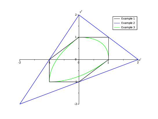
Before studying the domain of reflection, we introduce three examples in dimension $3$ of switching problems. On Figure 1, we draw the domain $\mathcal{D}_{\!\circ}$ for these three different switching problems to illustrate the impact of the various controlled randomisations on the shape of the reflecting domain.

Example 1:

Classical switching problem with a constant cost $1$, i.e. $\mathcal{C}=\{1,2\}$,

$$P^{1}=\left(\begin{array}[]{ccc}0&1&0\\ 0&0&1\\ 1&0&0\end{array}\right)\;,\;P^{2}=\left(\begin{array}[]{ccc}0&0&1\\ 1&0&0\\ 0&1&0\end{array}\right)\;,\;\bar{c}^{1}=\left(\begin{array}[]{c}1\\ 1\\ 1\\ \end{array}\right)\;\text{ and }\;\bar{c}^{2}=\left(\begin{array}[]{c}1\\ 1\\ 1\\ \end{array}\right).$$

Example 2:

Randomised switching problem with $\mathcal{C}=\{0\}$,

$$P^{0}=\left(\begin{array}[]{ccc}0&1/2&1/2\\ 1/2&0&1/2\\ 1/2&1/2&0\end{array}\right)\;\text{ and }\;\bar{c}^{0}=\left(\begin{array}[]{c}1\\ 1\\ 1\\ \end{array}\right).$$

Example 3:

Switching problem with controlled randomisation where $\mathcal{C}=[0,1]$,

$$P^{u}=\left(\begin{array}[]{ccc}0&u&1-u\\ 1-u&0&u\\ u&1-u&0\\ \end{array}\right)\;\text{ and }\;\bar{c}^{0}=\left(\begin{array}[]{c}1-u(1-u)\\ 1-u(1-u)\\ 1-u(1-u)\\ \end{array}\right)\quad\forall u\in[0,1].$$ (3.2)

In this example, the transitions matrix are given by convex combinations of transitions matrix of Example 1.

Figure 1: Domaine $\mathcal{D}_{\!\circ}$ for three examples of switching problems with or without controlled randomisation.

Remark 3.1.

For the randomised switching problem, in any dimension, we can replace $(P_{i,j})_{1\leq j\leq d}$ by $\left(\frac{P_{i,j}}{1-P_{i,i}}{\bf 1}_{i\neq j}\right)_{1\leq j\leq d}$ and $\bar{c}_{i}$ by $\frac{\bar{c}_{i}}{1-P_{i,i}}$ as soon as $P_{i,i}<1$, without changing $\mathcal{D}$. The factor $({1-P_{i,i}})^{-1}$ in the cost has to be seen as the expectation of the geometric law of the number of trials needed to exit state $i$. So assuming that diagonal terms are zero is equivalent to assume that $P_{i,i}<1$, for all $1\leq i\leq d$.

3.1.1 The uncontrolled case

In this part, we study the domain $\mathcal{D}$ for a fixed control, which is fixed to be $0$, without loss of generality. The properties of the domain are closely linked in this case to the homogeneous Markov chain, denoted $X$, associated to the stochastic matrix $P$. For this part, we thus work with the following assumption.

Assumption 3.1.

The set of control is reduced to $\mathcal{C}=\{0\}$. The Markov chain $X$ with stochastic matrix $P=(P_{i,j})_{1\leq i,j\leq d}:=(P^{0}_{i,j})_{1\leq i,j\leq d}$ is irreducible.

Our main goal is to find necessary and sufficient conditions to characterize the non-emptiness of the domain $\mathcal{D}$. To this end, we will introduce some quantities related to the Markov Chain $X$ and the costs vector $\bar{c}:=\bar{c}^{0}$.

For $1\leq i,j\leq d$, we consider the expected cost along an “excursion” from state $i$ to $j$:

$$\bar{C}_{i,j}:=\mathbb{E}\!\!\left[\sum_{n=0}^{\tau_{j}-1}\bar{c}_{X_{n}}\Big{|}X_{0}=i\right]{\color[rgb]{0,0,0}=\mathbb{E}\!\!\left[\sum_{n=0}^{\tau_{j}-1}c_{X_{n},X_{n+1}}\Big{|}X_{0}=i\right]}$$ (3.3)

where

$$\tau_{j}:=\inf\{t\geq 1\,|\,X_{t}=j\}\;.$$

We also define

$$C_{j,j}:=0\;\text{ and }\;C_{i,j}=\bar{C}_{i,j}\text{ for }1\leq i\neq j\leq d\;.$$ (3.4)

We observe that, introducing $\tilde{\tau}_{j}:=\inf\{t\geq 0\,|\,X_{t}=j\}$, the cost $C$ rewrites as $\bar{C}$:

$${C}_{i,j}:=\mathbb{E}\!\!\left[\sum_{n=0}^{\tilde{\tau}_{j}}\bar{c}_{X_{n}}{\bf 1}_{\{X_{n}\neq j\}}\Big{|}X_{0}=i\right]\;,\text{ for }1\leq i,j\leq d\,.$$

Let us remark that $\mathbb{E}\!\!\left[\tau+\tilde{\tau}\right]<+\infty$ and so $\bar{C}$ and $C$ are finite since the Markov chain is irreducible recurrent.
Setting $Q=I_{d}-P$, the domain $\mathcal{D}$, defined in (2.9), rewrites:

$$\mathcal{D} =\{x\in\mathbb{R}^{d}:Qx+c\succcurlyeq 0\}.$$ (3.5)

Since $P$ is irreducible, it is well known (see for example [3], Section 2.5) that for all $1\leq i,j\leq d$, the matrix $Q^{(i,j)}$ is invertible, and that we have

$$\tilde{\mu}_{i}:=\det Q^{(i,i)}=(-1)^{i+j}\det Q^{(i,j)}>0.$$ (3.6)

Moreover, $\tilde{\mu}Q=0$ with $\tilde{\mu}=(\tilde{\mu}_{i})_{i=1}^{d}$, i.e. ${\mu}:=\frac{\tilde{\mu}}{\sum_{i=1}^{d}\tilde{\mu}_{i}}$ is the unique invariant probability measure for the Markov chain with transition matrix $P$.

We now obtain some necessary conditions for the domain to be non-empty. Let us first observe that

Lemma 3.2.

The mean costs $C$ are given for $1\leq i\neq j\leq d$ by

$$C_{i,j}=\left((Q^{(j,j)})^{-1}\bar{c}^{(j)}\right)_{i-{\bf 1}_{\{i>j\}}}\;.$$ (3.7)

Proof. 1. We first show that for $1\leq i,j\leq d$:

$$\bar{C}_{i,j}=\bar{c}_{i}+\sum_{\ell\neq j}\bar{C}_{\ell,j}P_{i,\ell}\;.$$ (3.8)

From (3.3), we have

$$\bar{C}_{i,j} =\mathbb{E}\!\!\left[\sum_{n=0}^{+\infty}\bar{c}_{X_{n}}{\bf 1}_{\{n<\tau_{j}\}}\Big{|}X_{0}=i\right]=\bar{c}_{i}+\mathbb{E}\!\!\left[\sum_{n=1}^{+\infty}\bar{c}_{X_{n}}{\bf 1}_{\{n<\tau_{j}\}}\Big{|}X_{0}=i\right].$$

Then, since for all $n\geq 1$, $\{X_{1}=j\}\cap\{n<\tau_{j}\}=\emptyset$, we get

$$\bar{C}_{i,j} =\bar{c}_{i}+\mathbb{E}\!\!\left[\sum_{n=1}^{+\infty}\sum_{\ell\neq j}\bar{c}_{X_{n}}{\bf 1}_{\{X_{1}=\ell\}}{\bf 1}_{\{n<\tau_{j}\}}\Big{|}X_{0}=i\right].$$

We compute that, for $\ell\neq j$,

$$\mathbb{E}\!\!\left[\sum_{n=1}^{+\infty}\bar{c}_{X_{n}}{\bf 1}_{\{X_{1}=\ell\}}{\bf 1}_{\{n<\tau_{j}\}}\Big{|}X_{0}=i\right]=\mathbb{E}\!\!\left[\sum_{n=1}^{+\infty}\bar{c}_{X_{n}}{\bf 1}_{\{n<\tau_{j}\}}\Big{|}X_{1}=\ell\right]P_{i,\ell}.$$

The proof of (3.8) is then concluded observing that from the Markov property,

$$\mathbb{E}\!\!\left[\sum_{n=1}^{+\infty}\bar{c}_{X_{n}}{\bf 1}_{\{n<\tau_{j}\}}\Big{|}X_{1}=\ell\right]=\bar{C}_{\ell,j}\,.$$

2. From (3.8), we deduce, recall Definition (3.4), that, for $i\neq j$,

$${C_{i,j}}=\bar{c}_{i}+\sum_{\ell\neq j}{C}_{\ell,j}P_{i,\ell}\;.$$ (3.9)

This equality simply rewrites $Q^{(j,j)}C_{\cdot,j}=\bar{c}^{(j)}$, which concludes the proof. $\Box$

Proposition 3.1.

Assume $\mathcal{D}$ is non-empty. Then,

1. the mean cost with respect to the invariant measure is non-negative, namely:

   $${\mu}\bar{c}\geq 0.$$ (3.10)

2. For all $1\leq i,j\leq d$,

   $$\min_{1\leq i,j\leq d}\left(C_{i,j}+C_{j,i}\right)\geq 0.$$ (3.11)

3. The set $\mathcal{D}_{\!\circ}$ is compact in $\{y\in\mathbb{R}^{d}|y_{d}=0\}$.

Moreover, if $\mathcal{D}$ has non-empty interior, then

$$\mu\bar{c}>0\;\text{ and }\;\min_{1\leq i\neq j\leq d}\left(C_{i,j}+C_{j,i}\right)>0\;.$$ (3.12)

Proof. 1.a We first show the key relation:

$$-C_{i,j}\leq x_{i}-x_{j}\leq C_{j,i}\;,\;\text{ for }1\leq i,j\leq d.$$ (3.13)

For $j\in\{1,\dots,d\}$ and $x\in\mathbb{R}^{d}$, we introduce $\pi^{j}(x)\in\mathbb{R}^{d-1}$, given by,

$$\pi^{j}(x)_{k}=x_{k+{\bf 1}_{\{k\geq j\}}}-x_{j}\;,\;\;k\in\{1,\dots,d-1\}.$$

Let $x\in\mathcal{D}$ and $j\in\{1,\dots,d\}$. For all $i\in\{1,\dots,d\},i\neq j$, we have, by definition of $\mathcal{D}$ and since $\sum_{k=1}^{d}P_{i,k}=1$,

$$x_{i}-x_{j}\geq\sum_{k=1}^{d}P_{i,k}\left(x_{k}-x_{j}\right)-\bar{c}_{i}.$$

Thus $\pi_{j}(x)$ satisfies to

$$Q^{(j,j)}\pi^{j}(x)\succcurlyeq-\bar{c}^{(j)}.$$

Since $\left(Q^{(j,j)}\right)^{-1}=\sum_{k\geq 0}\left(P^{(j,j)}\right)^{k}\succcurlyeq 0$, we obtain, using inequality (3.7)

$$\pi^{j}(x)\succcurlyeq-\left(Q^{(j,j)}\right)^{-1}\bar{c}^{(j)}=-C^{(j)}_{\cdot,j},$$ (3.14)

which means $x_{i}-x_{j}\geq-C_{i,j}$ for all $i\neq j$.
Let $1\leq i\neq j\leq d$. The precedent reasoning gives $x_{i}-x_{j}\geq-C_{i,j}$ and $x_{j}-x_{i}\geq-C_{j,i}$, thus (3.13) is proved.
From (3.13), we straightforwardly obtain (3.11) and the fact that $\mathcal{D}_{\!\circ}$ is compact in $\{y\in\mathbb{R}^{d}:y_{d}=0\}$.
1.b Since $\mathcal{D}$ is non empty, the following holds for some $x\in\mathbb{R}^{d}$, recalling (3.5),

$$Qx+\bar{c}\succcurlyeq 0$$

Multiplying by ${\mu}$ the previous inequality, we obtain (3.10), since ${\mu}Q=0$.
2. Assume now that $\mathcal{D}$ has non-empty interior and consider $x\in\overset{\circ}{\mathcal{D}}$. Then, for all $1\leq i\leq d$, we have that $x-\epsilon e_{i}$ belongs to $\mathcal{D}$ for $\epsilon>0$ small enough. Thus, we get

$$x_{i}-\epsilon\geq\sum_{\ell=1}^{d}P_{i,\ell}x_{\ell}-\epsilon P_{i,i}-\bar{c}_{i}$$

and then

$$Qx+\bar{c}\succcurlyeq\epsilon\min_{1\leq i\leq d}(1-P_{i,i})\sum_{\ell=1}^{d}e_{\ell}.$$

Since $P$ is irreducible, $\min_{1\leq i\leq d}(1-P_{i,i})>0$, and multiplying by ${\mu}$ both sides of the previous inequality we obtain ${\mu}\bar{c}>0$.
For any $j\neq i$, since $x-\epsilon e_{i}\in\mathcal{D}$, we deduce from (3.13), $-C_{i,j}+\epsilon\leq x_{i}-x_{j}$. Using again (3.13), we get $-C_{i,j}+\epsilon\leq C_{j,i}$. This proves the right hand side of (3.12). $\Box$

The next lemma, whose proof is postponed to Appendix A.1, links the condition (3.10) to costly round-trip.

Lemma 3.3.

The followings hold, for $1\leq j\leq d$,

$$\bar{C}_{jj}=\frac{\mu\bar{c}}{\mu_{j}}\;,$$ (3.15)

and, for $1\leq i\neq j\leq d$,

$$C_{i,j}+C_{j,i}=\frac{\mu\bar{c}}{\mu_{i}}\left(\left[Q^{(j,j)}\right]^{-1}\right)_{i^{(j)},i^{(j)}}\;.$$ (3.16)

We are now going to show that previous necessary conditions are also sufficient. The main result of this section is thus the following.

Theorem 3.1.

The following conditions are equivalent:

1. The domain $\mathcal{D}$ is non-empty (resp. has non-empty interior).

2. There exists $1\leq i\neq j\leq d$ such that $C_{i,j}+C_{j,i}\geq 0$ (resp. $C_{i,j}+C_{j,i}>0$).

3. The inequality $\mu\bar{c}\geq 0$ (resp. $\mu\bar{c}>0$) is satisfied.

4. For all $1\leq i\neq j\leq d$, $C_{i,j}+C_{j,i}\geq 0$ (resp. $C_{i,j}+C_{j,i}>0$).

Proof. 1 We first note that in Proposition 3.1 we have proved $i)\implies iv)$. We also remark that $iv)\implies ii)$ trivially, and $ii)\implies iii)$ in a straightforward way from equality (3.16), recalling that $\left(Q^{(j,j)}\right)^{-1}=\sum_{k\geq 0}\left(P^{(j,j)}\right)^{k}\succcurlyeq 0$.
2. We now study $iii)\implies i)$.
2.a Assume that $\mu\bar{c}\geq 0$. For $1\leq j\leq d$, we denote $z^{j}:=-C_{\cdot,j}$. Then from (3.9), we straightforwardly observe that, for all $i\neq j$,

$$z^{j}_{i}=\sum_{\ell=1}^{d}z^{j}_{\ell}P_{i,\ell}-\bar{c}_{i}\;.$$ (3.17)

We now take care of the case $i=j$ by computing, recall $z^{j}_{j}=0$,

$$z^{j}_{j}-\sum_{\ell=1}^{d}z^{j}_{\ell}P_{j,\ell}+\bar{c}_{j} =\sum_{\ell=1}^{d}C_{\ell,j}P_{j,\ell}+\bar{c}_{j}=\bar{C}_{j,j}$$ (3.18)

where we used (3.8) with $i=j$. Then, combining (3.15) and the assumption $\mu\bar{c}\geq 0$ for this step, we obtain that $z^{j}\in\mathcal{D}$ and so $\mathcal{D}$ is non empty.
2.b We assume that $\mu\bar{c}>0$ which implies that $\bar{C}_{jj}=\frac{\mu\bar{c}}{\mu_{j}}>0$ for all $1\leq j\leq d$ recalling (3.15). Set any $j\in\{1,\dots,d\}$ and consider $z^{j}:=-C_{\cdot,j}$ introduced in the previous step. We then set

$$x:=z^{j}+\frac{1}{2(d-1)}\sum_{k\neq j}(z^{k}-z^{j}).$$ (3.19)

Next, we compute, for $i\neq j$, recalling (3.17) and (3.18),

$$\left(Qx+\bar{c}\right)_{i} =\left(Qz^{j}+\bar{c}\right)_{i}+\frac{1}{2(d-1)}\sum_{k\neq j}(Qz^{k}-Qz^{j})_{i}$$

$$=0+\frac{1}{2d}(Qz^{i}-Qz^{j})_{i}=\frac{1}{2(d-1)}((Qz^{i})_{i}+\bar{c}_{i})=\bar{C}_{i,i}>0.$$

For $i=j$, we compute, recalling (3.17) and (3.18),

$$\left(Qx+\bar{c}\right)_{j} =\left(Qz^{j}+\bar{c}\right)_{j}+\frac{1}{2(d-1)}\sum_{k\neq j}(Qz^{k}-Qz^{j})_{j}$$

$$=\bar{C}_{j,j}+\frac{1}{2(d-1)}\sum_{k\neq j}(-\bar{c}_{j}+\bar{c}_{j}-\bar{C}_{j,j})=\frac{\bar{C}_{j,j}}{2}>0.$$

Combining the two previous inequalities, we obtain that

$$Qx+\bar{c}\succcurlyeq\frac{\delta}{2}{\bf 1}\,\quad\text{with}\quad\delta=\min\{\bar{C}_{i,i}|1\leq i\leq d\}.$$

From this, we easily deduce that $x+B(0,\frac{\delta}{4\sup_{i}||Q_{i,\cdot}||_{2}})\subset\mathcal{D}$, which proves that $\mathcal{D}$ has a non-empty interior.
$\Box$

We now give some extra conditions that are linked to the non-emptiness of the domain $\mathcal{D}$

Proposition 3.2.

The following assertions are equivalent:

1. $\mathcal{D}$ is non-empty,

2. For all $1\leq i,j,k\leq d$, the following holds

   $$C_{jk}\leq C_{ji}+C_{ik},$$ (3.20)

3. For any round trip of length less than $d$, i.e. $1\leq n\leq d$, $1\leq i_{1}\neq...\neq i_{n}\leq d$, we have

   $${\sum_{k=1}^{n-1}C_{i_{k},i_{k+1}}+C_{i_{n},i_{1}}\geq 0}.$$ (3.21)

Proof. 1. $i)\implies ii)$. From Theorem 3.1, we know that $-C_{\cdot,k}\in\mathcal{D}$ for all $k\in\{1,\dots,d\}$. Using then (3.13), we have

$$-C_{i,k}+C_{j,k}\leq C_{j,i}\;,\text{ for all}1\leq i,j\leq d\;,$$

which concludes the proof for this step.
2. $ii)\implies iii)$ directly since $C_{i,i}=0$ for all $1\leq i\leq d$. Finally $iii)\implies i)$ is already proved in Theorem 3.1 for $2$-state round trip. $\Box$

Proposition 3.3.

Let us assume that $\mathcal{D}$ has a non empty interior. Define $\theta_{\cdot,j}=C_{\cdot,j}-C_{d,j}{\bf 1}$, for all $1\leq j\leq d$. Then $(-\theta_{\cdot,j})_{1\leq j\leq d}$ are affinely independent and $\mathcal{D}_{\!\circ}$ is the convex hull of these points.

Proof. We know from Step 2.a in the proof of Theorem 3.1 that $-C_{\cdot,j}\in\mathcal{D}$ for all $1\leq j\leq d$. The invariance by translation along ${\bf 1}$ of the domain proves that $-\theta_{\cdot,j}$ are in $\mathcal{D}_{\!\circ}$. More precisely, we obtain from (3.9) that,

$$\theta_{i,j}-\sum_{\ell=1}^{d}\theta_{\ell,j}P_{i,\ell}=\bar{c}_{i}\;,\quad\text{ for }1\leq i\neq j\leq d\;.$$ (3.22)

1. We now prove that $(\theta_{\cdot,j})_{1\leq j\leq d}$ are affinely independent. We consider thus $\alpha\in\mathbb{R}^{d}$ such that

$$\sum_{j=1}^{d}\alpha_{j}=0\quad\text{ and }\quad z:=\sum_{j=1}^{d}\alpha_{j}\theta_{\cdot,j}=0\;.$$ (3.23)

and we aim to prove that $\alpha_{j}=0$, for $j\in\{1,\dots,d\}$. To this end, we compute, for $i\in\{1,\dots,d\}$,

$$z_{i}:=\sum_{j=1}^{d}\alpha_{j}\theta_{i,j} =\sum_{j\neq i}\alpha_{j}\theta_{i,j}+\alpha_{i}\theta_{ii}=\sum_{j\neq i}\alpha_{j}\bar{c}_{i}+\sum_{\ell=1}^{d}\sum_{j\neq i}\alpha_{j}\theta_{\ell,j}P_{i,\ell}-\alpha_{i}C_{d,i}$$

$$=\sum_{j\neq i}\alpha_{j}\bar{c}_{j}+\sum_{\ell=1}^{d}z_{\ell}P_{i,\ell}-\alpha_{i}\sum_{\ell=1}^{d}\theta_{\ell,i}P_{i,\ell}-\alpha_{i}C_{d,i}$$

$$=-\alpha_{i}(\bar{c}_{i}+\sum_{\ell=1}^{d}\theta_{\ell,i}P_{i,\ell}+C_{d,i})=-\alpha_{i}(\bar{c}_{i}+\sum_{\ell=1}^{d}C_{\ell,i}P_{i,\ell})=-\alpha_{i}\bar{C}_{i,i}.$$

We thus deduce that $\alpha_{i}=0$ since $\bar{C}_{i,i}=\frac{\mu\bar{c}}{\mu_{i}}>0$, which concludes the proof for this step.
2. We now show that $\mathcal{D}_{\!\circ}$ is the convex hull of points $(-\theta_{\cdot,j})_{1\leq j\leq d}$, which are affinely independent from the previous step. For $y\in\mathbb{R}^{d}\cap\{y_{d}=0\}$, there exists thus a unique $(\lambda_{1},\dots,\lambda_{d-1})\in\mathbb{R}^{d-1}$ such that $y=\sum_{j=1}^{d}-\lambda_{j}\theta_{\cdot,j}$, with $\lambda_{d}=1-\sum_{j=1}^{d-1}\lambda_{j}$. Assuming that $y\in\mathcal{D}$, we have that

$$v:=Qy+\bar{c}=\sum_{j=1}^{d}-\lambda_{j}Q\theta_{\cdot,j}+\bar{c}=\sum_{j=1}^{d}\lambda_{j}[Q(-\theta_{.,j})+\bar{c}]\succcurlyeq 0\;.$$

Since $[Q(-\theta_{.,j})+\bar{c}]_{i}=0$ for all $i\neq j$, we get, for all $1\leq i\leq d$,

$$v_{i}=\lambda_{i}([Q(-\theta_{.,i})]_{i}+\bar{c}_{i})\geq 0.$$

Recalling that $[Q(-\theta_{.,i})]_{i}+\bar{c}_{i}\geq 0$ we obtain $\lambda_{i}\geq 0$ which concludes the proof. $\Box$

3.1.2 The setting of controlled randomisation

In this part we adapt Assumption 3.1 in the following natural way.

Assumption 3.2.

For all $u\in\mathcal{C}$, the Markov chain with stochastic matrix $P^{u}:=(P^{u}_{i,j})_{1\leq i,j\leq d}$ is irreducible.

We then consider the matrix $\widehat{C}$ defined by, for all $(i,j)\in\{1,\dots,d\}$

$$\widehat{C}_{i,j}:=\min_{u\in\mathcal{C}}{C}^{u}_{i,j}\,\,$$ (3.24)

recall the Definition of $\bar{C}^{u}_{i,j}$ for a fixed control in (3.3). Let us note that $\widehat{C}_{i,j}$ is well defined in $\mathbb{R}$ under Assumption 3.2 since $\mathcal{C}$ is compact.

The following result is similar as Proposition 3.1 but in the context of switching with controlled randomisation.

Proposition 3.4.

Assume $\mathcal{D}$ is non-empty (resp. has non-empty interior). Then,

$$\min_{u}\mu^{u}\bar{c}^{u}\geq 0\;(\text{resp.}>0)\quad\text{ and }\quad\min_{1\leq i\neq j\leq d}\left(\widehat{C}_{i,j}+\widehat{C}_{j,i}\right)\geq 0\;(\text{resp.}>0)\;.$$ (3.25)

Moreover, the set $\mathcal{D}_{\!\circ}$ is compact in $\{y\in\mathbb{R}^{d}:y_{d}=0\}$.

Proof. 1. Let $x\in\mathcal{D}$. From (3.13), we have for each $u\in\mathcal{C}$, $-C^{u}_{i,j}\leq x_{i}-x_{j}\leq C^{u}_{j,i}\;.$ Minimizing on $u\in\mathcal{C}$, we then obtain

$$-\widehat{C}_{i,j}\leq x_{i}-x_{j}\leq\widehat{C}_{j,i}\;.$$ (3.26)

From this, we deduce that $\mathcal{D}_{\!\circ}$ is compact in $\{y\in\mathbb{R}^{d}:y_{d}=0\}$ and we get the right handside of (3.25).
We also have that, for all $u\in\mathcal{C}$,

$$Q^{u}x+\bar{c}^{u}\succcurlyeq 0\,,$$

then multiplying by $\mu^{u}$ we obtain $\mu^{u}\bar{c}^{u}\geq 0$. This leads to $\min_{u}\mu^{u}\bar{c}^{u}\geq 0$.
2. Then, results concerning the non-empty interior framework can be obtained as in the proof of Proposition 3.1.

The case of controlled costs only.

Let us first start by introducing the minimal controlled mean cost:

$$\hat{c}_{i}:=\min_{u\in\mathcal{C}}\bar{c}^{u}_{i}\;,\quad\text{for}\;1\leq i\leq d\;.$$

In this setting, we have that

$$\mathcal{D}:= \{x\in\mathbb{R}^{d}:(Qx)_{i}+\bar{c}^{u}_{i}\geq 0\;,\text{for all }u\in\mathcal{C},\;1\leq i\leq d\}$$

$$= \{x\in\mathbb{R}^{d}:(Qx)_{i}+\hat{c}_{i}\geq 0\;,\text{for all }\;1\leq i\leq d\}.$$

Using the result of Proposition 3.1 with the new costs $\hat{c}$, we know that a necessary and sufficient condition is $\mu\hat{c}\geq 0$. Moreover, the matrix $C$ is defined here by

$$C_{i,j}=\left((Q^{(j,j)})^{-1}\hat{c}^{(j)}\right)_{i-{\bf 1}_{\{i>j\}}},\quad 1\leq i\neq j\leq d\;,$$ (3.27)

and $C_{i,i}=0$, for $1\leq i\leq d$. Comparing the above expression with the definition of $\widehat{C}$ in (3.24), we observe that $C_{i,j}\leq\widehat{C}_{i,j}$, $1\leq i,j\leq d$. The following example confirms that

$$\min_{1\leq i\neq j\leq d}\left(\widehat{C}_{i,j}+\widehat{C}_{j,i}\right)\geq 0\,,$$

recall Proposition 3.4, is not a sufficient condition in this context for non-emptiness of the domain.

Example 3.1.

Set $\mathcal{C}=\{0,1\}$,

$$P=\left(\begin{array}[]{ccc}0&0.5&0.5\\ 0.5&0&0.5\\ 0.5&0.5&0\end{array}\right)\;,\;\bar{c}^{0}=\left(\begin{array}[]{c}-0.5\\ 1.2\\ 0.7\\ \end{array}\right)\;\text{ and }\;\bar{c}^{1}=\left(\begin{array}[]{c}1.5\\ 0.2\\ 0.2\\ \end{array}\right)$$

Observe that $\mu=(\frac{1}{3},\frac{1}{3},\frac{1}{3})$ and $\hat{c}=(-0.5,0.2,0.2)^{\top}$. Then, one computes that

$$\min_{1\leq i\neq j\leq d}\left(\widehat{C}_{i,j}+\widehat{C}_{j,i}\right)>0\quad\text{ but }\quad\mu\hat{c}<0\;.$$

3.2 The Markovian framework

We now introduce a Markovian framework, and prove that a solution to (2.6)-(2.7)-(2.8) exists for the randomised switching problem under Assumption 3.1 and a technical copositivity hypothesis, see Assumption 3.4 below. We also investigate an example of switching problem with controlled randomisation, see (3.2).
To this effect, we rely on the existence theorem obtained in [7], which we recall next. For all $(t,x)\in[0,T]\times\mathbb{R}^{q}$, let $X^{t,x}$ be the solution to the following SDE:

$$\mathrm{d}X_{s} =b(s,X_{s})\mathrm{d}s+\sigma(s,X_{s})\mathrm{d}W_{s},s\in[t,T],$$ (3.28)

$$X_{t} =x.$$ (3.29)

We are interested in the solutions $(Y^{t,x},Z^{t,x},K^{t,x})\in\mathbb{S}^{2}_{d}(\mathbb{F}^{0})\times\mathbb{H}^{2}_{d\times\kappa}(\mathbb{F}^{0})\times\mathbb{A}^{2}_{d}(\mathbb{F}^{0})$ of (2.6)-(2.7)-(2.8), where the terminal condition satisfies $\xi=g(X^{t,x}_{T})$, and the driver satisfies $f(\omega,s,y,z)=\psi(s,X^{t,x}_{s}(\omega),y,z)$ for some deterministic measurable functions $g,\psi$. We next give the precise set of assumptions we need to obtain our results.

For sake of completeness, we recall here the existence result proved in [7], see also [9].

Assumption 3.3.

There exist $p\geq 0$ and $L\geq 0$ such that

1. $$|\psi(t,x,y,z)|\leq L(1+|x|^{p}+|y|+|z|).$$

   Moreover, $\psi(t,x,\cdot,\cdot)$ is continuous on $\mathbb{R}^{d}\times\mathbb{R}^{d\times\kappa}$ for all $(t,x)\in[0,T]\times\mathbb{R}^{q}$.

2. $(b,\sigma):[0,T]\times\mathbb{R}^{q}\to\mathbb{R}^{q}\times\mathbb{R}^{q\times\kappa}$ is a measurable function satisfying, for all $(t,x,y)\in[0,T]\times\mathbb{R}^{q}\times\mathbb{R}^{q}$,

   $$|b(t,x)|+|\sigma(t,x)| \leq L(1+|x|),$$

   $$|b(t,x)-b(t,y)|+|\sigma(t,x)-\sigma(t,y)| \leq L|x-y|.$$

3. $g:\mathbb{R}^{q}\to\mathbb{R}^{d}$ is measurable and for all $(t,x)\in[0,T]\times\mathbb{R}^{q}$, we have

   $$|g(t,x)|\leq L(1+|x|^{p}).$$

4. Let $\mathcal{X}=\{\mu(t,x;s,dy),x\in\mathbb{R}^{q}\textrm{ and }0\leq t\leq s\leq T\}$ be the family of laws of $X^{t,x}$ on $\mathbb{R}^{q}$, i.e., the measures such that $\forall A\in\mathcal{B}(\mathbb{R}^{q})$, $\mu(t,x;s,A)=\mathbb{P}(X_{s}^{t,x}\in A)$. For any $t\in[0,T)$, for any $\mu(0,a;t,dy)$-almost every $x\in\mathbb{R}^{q}$, and any $\delta\in]0,T-t]$, there exists an application $\phi_{t,x}:[t,T]\times\mathbb{R}^{d}\rightarrow\mathbb{R}_{+}$ such that:

   1. $\forall k\geq 1$, $\phi_{t,x}\in L^{2}([t+\delta,T]\times[-k,k]^{q};\mu(0,a;s,dy)ds)$,

   2. $\mu(t,x;s,dy)ds=\phi_{t,x}(s,y)\mu(0,a;s,dy)ds$ on $[t+\delta,T]\times\mathbb{R}^{q}$.

5. $H:\mathbb{R}^{d}\to\mathbb{R}^{d\times d}$ is a measurable function, and there exists $\eta>0$ such that, for all $(y,y^{\prime})\in\mathcal{D}\times\mathbb{R}^{d}$ and $v\in\mathfrak{n}(\mathfrak{P}(y))$, where $\mathfrak{P}$ is the projection on $\mathcal{D}$, we have

   $$v^{\top}H(y)v \geq\eta,$$

   $$|H(y^{\prime})| \leq L.$$

   Moreover, $H$ is continuous on $\mathcal{D}$.

Remark 3.2.

Assumption iv) is true as soon as $\sigma$ is uniformly elliptic, see [15].

The existence result in the Markovian setting reads as follows.

Theorem 3.2 ([7], Theorem 4.1).

Under Assumption 3.3, there exists a solution $(Y^{t,x},Z^{t,x},\Psi^{t,x})\in\mathbb{S}^{2}_{d}(\mathbb{F}^{0})\times\mathbb{H}^{2}_{d\times\kappa}(\mathbb{F}^{0})\times\mathbb{H}^{2}_{d}(\mathbb{F}^{0})$ of the following system

$$Y_{s} =g(X^{t,x}_{T})+\int_{s}^{T}\!\!\!\!\psi(u,X^{t,x}_{u},Y_{u},Z_{u})\mathrm{d}u-\int_{s}^{T}\!\!\!Z_{u}\mathrm{d}W_{u}-\int_{s}^{T}\!\!\!\!H(Y_{u})\Psi_{u}\mathrm{d}u,s\in[t,T],$$ (3.30)

$$Y_{s} \in\mathcal{D},\mbox{ }\Psi_{s}\in\mathcal{C}(Y_{s}),\mbox{ }t\leq s\leq T,$$ (3.31)

$$\int_{t}^{T} 1_{\{Y_{s}\not\in\partial\mathcal{D}\}}|\Psi_{s}|\mathrm{d}s=0.$$ (3.32)

The main point to invoke Theorem 3.2 is then to construct a function $H:\mathbb{R}^{d}\to\mathbb{R}^{d\times d}$ which satisfies Assumption 3.3 v) and such that

$$H(y)v\in\mathcal{C}_{o}(y),$$ (3.33)

for all $y\in\mathcal{D}$ and $v\in\mathcal{C}(y)$, where $\mathcal{C}_{o}(y)$ is the cone of directions of reflection, given here by

$$\mathcal{C}_{o}(y):=-\sum_{i=1}^{d}\mathbb{R}_{+}e_{i}1_{\left\{y_{i}=\max_{u\in\mathcal{C}}\left\{\sum_{j=1}^{d}P^{u}_{i,j}y_{j}-\bar{c}_{i}^{u}\right\}\right\}}.$$

If Assumption 3.3 i), ii), iii), iv) are also satisfied, we obtain the existence of a solution to (3.30)-(3.31)-(3.32). Setting $K^{t,x}_{s}:=-\int_{t}^{s}H(Y^{t,x}_{u})\Psi^{t,x}_{u}\mathrm{d}u$ for $t\leq s\leq T$ shows that $(Y^{t,x},Z^{t,x},K^{t,x})$ is a solution to (2.6)-(2.7)-(2.8).

3.2.1 Well-posedness result in the uncontrolled case

We assume here Assumption 3.1. In addition, we need to introduce the following technical assumption in order to construct $H$ satisfying Assumption 3.3 v) and (3.33).

Assumption 3.4.

For all $1\leq i\leq d$, the matrix $Q^{(i,i)}$ is strictly copositive, meaning that for all $0\preccurlyeq x\in\mathbb{R}^{d-1},x\neq 0$, we have

$$x^{\top}Q^{(i,i)}x>0.$$ (3.34)

Our main result for this section is the following theorem.

Theorem 3.3.

Suppose that Assumption 3.3 i), ii), iii), iv), Assumption 3.1 and Assumption 3.4 are satisfied and that $\mathcal{D}$ has non-empty interior.

Then, there exists $H:\mathbb{R}^{d}\to\mathbb{R}^{d\times d}$ satisfying 3.3 v). Consequently, there exists a solution to (2.6)-(2.7)-(2.8) with $\xi=g(X_{T})$ and $f(\omega,s,y,z)=\psi(s,X^{t,x}_{s}(\omega),y,z)$. Moreover this solution is unique if we assume also Assumption 2.1-ii).

Proof. We first observe that uniqueness follows from Proposition 2.1. We now focus on proving existence of solution which amounts to exhibit a convenient $H$ function. The general idea is to start by constructing $H$ on the points $(y^{i})_{1\leq i\leq d}$, given by

$$y^{i} :=(C_{d,i}-C_{j,i})_{1\leq j\leq d},$$ (3.35)

then, using Proposition 3.3, we can extend it on the whole $\mathcal{D}_{\!\circ}$ by linear combination, and finally we extend $H$ on all $\mathbb{R}^{d}$ by using the geometry of $\mathcal{D}$.
The proof is then divided into several steps.
1. We start by computing the outward normal cone $\mathcal{C}(y)$ for all $y\in\mathcal{D}_{\!\circ}$. Let us set $y\in\mathcal{D}_{\!\circ}$. Thanks to Proposition 3.3, there exists a unique $(\lambda_{i})_{1\leqslant i\leqslant d}\in[0,1]^{d}$ such that

$$y=\sum_{i=1}^{d}\lambda_{i}y^{i},\quad\sum_{i=1}^{d}\lambda_{i}=1.$$

Let us denote $\mathcal{E}_{y}=\{1\leqslant i\leqslant d|\lambda_{i}>0\}$. We will show that

$$\mathcal{C}(y)=\sum_{j\notin\mathcal{E}_{y}}\mathbb{R}_{+}n_{j}.$$ (3.36)

where $n_{i}:=(-Q_{i,j})_{1\leq j\leq d},$and with the convention $\mathcal{C}(y)=\emptyset$ when $\mathcal{E}_{y}=\{1,...,d\}$. Let us remark that the result is obvious when $\mathcal{C}(y)=\emptyset$, since, in this case, $y$ is in the interior of $\mathcal{D}$. So we will assume in the following that $\mathcal{C}(y)\neq\emptyset$.
1.a. First, let us show that for any $1\leqslant i\leqslant d$, $(n_{j})_{j\neq i}$ is a basis of $\{y\in\mathbb{R}^{d}|\sum_{k=1}^{d}v_{k}=0\}$. Let $1\leq i\neq j\leq d$. It is clear that $n_{j}\in\{v\in\mathbb{R}^{d}:\sum_{k=1}^{d}v_{k}=0\}$. Since it is a hyperplan of $\mathbb{R}^{d}$ and that the family $(n_{j})_{j\neq i}$ has $d-1$ elements, it is enough to show that the vectors are linearly independent. We observe that the matrix whose lines are the $n^{(i)}_{j},j\neq i,$ is $-Q^{(i,i)}$. Since $P$ is irreducible, $Q^{(i,i)}$ is invertible. The vectors $n^{(i)}_{j},j\neq i$ form a basis of $\mathbb{R}^{d-1}$, hence the vectors $(n_{j})_{j\neq i}$ form a basis of $\{v\in\mathbb{R}^{d}|\sum_{k=1}^{d}v_{k}=0\}$.
1.b. We set now $j\notin\mathcal{E}_{y}$ and we will show that $n_{j}\in\mathcal{C}(y)$. For any $z\in\mathcal{D}$, by definition of $\mathcal{D}$, we have

$$\bar{c}_{j}\geq\sum_{k=1}^{d}P_{j,k}z_{k}-z_{j}=n_{j}^{\top}z,$$

and for all $i\in\mathcal{E}_{y}$, by definition of $y^{i}$, we have

$$\bar{c}_{j}=\sum_{k=1}^{d}P_{j,k}y^{i}_{k}-y^{i}_{j}=n_{j}^{\top}y^{i}.$$

This gives $n_{j}^{\top}(z-y)=n_{j}^{\top}z-\sum_{i\in\mathcal{E}_{y}}\lambda_{i}n_{j}^{\top}y^{i}\leq 0$, hence $n_{j}\in\mathcal{C}(y)$.
1.c. We now set $i=\min\mathcal{E}_{y}$. Conversely, since $(n_{j})_{j\neq i}$ is a basis of $\{v\in\mathbb{R}^{d}:\sum_{i=1}^{d}v_{i}=0\}\ni\mathcal{C}(y)$, see Lemma 3.1, for $v\in\mathcal{C}(y)$ there exists a unique $\alpha=(\alpha_{j})_{j\neq i}\in\mathbb{R}^{d-1}$ such that $v=\sum_{j\neq i}\alpha_{j}n_{j}=(n_{j})_{j\neq i}\alpha$. We will show here that $\alpha_{\ell}=0$ for all $\ell\in\mathcal{E}_{y}\setminus\{i\}$ and $\alpha_{\ell}\geq 0$ for all $\ell\notin\mathcal{E}_{y}$.
For all $z\in\mathcal{D}$, previous calculations give us:

$$0 \geq\alpha^{\top}\left[(n_{j})_{j\neq i}\right]^{\top}(z-y)=-\alpha^{\top}Q^{(i,\cdot)}(z-\sum_{\ell\in\mathcal{E}_{y}}\lambda_{\ell}y^{\ell})=-\alpha^{\top}\left[Q^{(i,\cdot)}z-\sum_{\ell\in\mathcal{E}_{y}}\lambda_{\ell}Q^{(i,\cdot)}y^{\ell}\right].$$

Let us recall that for any $j\neq i$, by definition of $y^{j}$, one gets $Q^{(i,\cdot)}y^{j}+\bar{c}^{(i)}=\frac{\mu\bar{c}}{\mu_{j}}e_{j}$, and $Q^{(i,\cdot)}y^{i}+\bar{c}^{(i)}=0$. Thus, previous inequality becomes

$$0 \leq\alpha^{\top}\left[Q^{(i,\cdot)}z-\sum_{\ell\in\mathcal{E}_{y}\setminus\{i\}}\lambda_{\ell}\left(\frac{\mu\bar{c}}{\mu_{\ell}}e_{\ell}-\bar{c}^{(i)}\right)+\lambda_{i}\bar{c}^{(i)}\right]$$

$$=\alpha^{\top}\left[Q^{(i,\cdot)}z+\bar{c}^{(i)}-\sum_{\ell\in\mathcal{E}_{y}\setminus\{i\}}\lambda_{\ell}\frac{\mu\bar{c}}{\mu_{\ell}}e_{\ell}\right].$$ (3.37)

By taking $z=y^{j}$ in (3.37), with $j\in\mathcal{E}_{y}\setminus\{i\}$, we get

$$0 \leq\alpha^{\top}\left[\frac{\mu\bar{c}}{\mu_{j}}e_{j}-\sum_{\ell\in\mathcal{E}_{y}\setminus\{i\}}\lambda_{\ell}\frac{\mu\bar{c}}{\mu_{\ell}}e_{\ell}\right]$$ (3.38)

and so, we can sum, over $j$, previous inequality with positive weights $\alpha_{j}$, to obtain

$$0 \leq\left(1-\sum_{j\in\mathcal{E}_{y}\setminus\{i\}}\lambda_{j}\right)\alpha^{\top}\left[\sum_{\ell\in\mathcal{E}_{y}\setminus\{i\}}\lambda_{\ell}\frac{\mu\bar{c}}{\mu_{\ell}}e_{\ell}\right].$$

Then $0\leq\alpha^{\top}\left[\sum_{\ell\in\mathcal{E}_{y}\setminus\{i\}}\lambda_{\ell}\frac{\mu\bar{c}}{\mu_{\ell}}e_{\ell}\right]$ since $\lambda_{i}>0$. Moreover, we have also $0\geq\alpha^{\top}\left[\sum_{\ell\in\mathcal{E}_{y}\setminus\{i\}}\lambda_{\ell}\frac{\mu\bar{c}}{\mu_{\ell}}e_{\ell}\right]$ by taking $z=y^{i}$ in (3.37), which gives us that

$$\alpha^{\top}\left[\sum_{\ell\in\mathcal{E}_{y}\setminus\{i\}}\lambda_{\ell}\frac{\mu\bar{c}}{\mu_{\ell}}e_{\ell}\right]=0.$$ (3.39)

We recall that $\mu\bar{c}>0$ since $\mathcal{D}$ has non-empty interior (see Theorem 3.1). Pluging (3.39) in (3.38) gives us that $\alpha_{j}\geq 0$ for all $j\in\mathcal{E}_{y}\setminus\{i\}$, which, combined with (3.39) allows to conclude to $\alpha_{j}=0$ for all $j\in\mathcal{E}_{y}\setminus\{i\}$.
Now we apply (3.37) with $z=y^{j}$ for $j\notin\mathcal{E}_{y}$: hence $0\leqslant\alpha_{j}\frac{\mu\bar{c}}{\mu_{j}}$ for all $j\notin\mathcal{E}_{y}$, which concludes the proof of (3.36).
2. Then, we construct $H(y)$. Let us start by $H(y^{i})$ for any $1\leq i\leq d$. Fix $1\leq i\leq d$, and let $B^{i}\in\mathbb{R}^{(d-1)\times(d-1)}$ be the base change matrix from $(-n_{j}^{(i)})_{j\neq i}$ to the canonical basis of $\mathbb{R}^{d-1}$. We set $H(y^{i}):=I^{i}B^{i}P^{i}$, with $I^{i}:\mathbb{R}^{d-1}\to\mathbb{R}^{d}$ and $P^{i}:\mathbb{R}^{d}\to\mathbb{R}^{d-1}$ the linear maps defined by

$$I^{i}(x_{1},\dots,x_{d-1}) =(x_{1},\dots,x_{i-1},0,x_{i},\dots,x_{d-1}),$$ (3.40)

$$P^{i}(x_{1},\dots,x_{d}) =(x_{1},\dots,x_{i-1},x_{i+1},\dots,x_{d}).$$ (3.41)

Now we set $H(y):=\sum_{i\in\mathcal{E}_{y}}\lambda_{i}H(y^{i})$. Let us take $v\in\mathcal{C}(y)$. Thanks to (3.36), we know that $v=\sum_{j=1}^{d}\alpha_{j}n_{j}$ for some $(\alpha_{j})_{1\leq j\leq d}\in(\mathbb{R}^{+})^{d}$ and such that $\alpha_{j}=0$ when $j\in\mathcal{E}_{y}$. Since $n_{k}=-Q_{k}^{\top}$, for all $1\leq k\leq d$, we have $v=-Q^{\top}\alpha$. By construction, we get that

$$H(y)v=-\sum_{j\notin\mathcal{E}_{y}}\alpha_{j}e_{j}=-\alpha\in\mathcal{C}_{o}(y).$$

It remains to check that Assumption 3.3-v) is fulfilled. If $v\neq 0$, which is equivalent to $\alpha\neq 0$, we have, for $i\in\mathcal{E}_{y}$,

$$v^{\top}H(y)v=\alpha^{\top}Q\alpha=(\alpha^{(i)})^{\top}Q^{(i,i)}\alpha^{(i)}>0,$$

due to Assumption 3.4 and the fact that $\alpha_{i}=0$.
3. We have constructed $H$ on $\mathcal{D}_{\!\circ}$ with needed properties. Finally, we set $H(x)=H(x-x_{d}\sum_{i=1}^{d}e_{i})$ for all $x\in\mathcal{D}$ and $H(x)=H(\mathfrak{P}(x))$ for $x\in\mathbb{R}^{d}$ and the proof is finished. $\Box$

Remark 3.3.

i) Assumption 3.4 is satisfied as soon as $P$ is symmetric and irreducible. Indeed, $Q^{(i,i)}$ is then nonsingular, symmetric and diagonally dominant, hence positive definite, for all $i\in\{1,\dots,d\}$.
ii) In dimension $3$, if $P$ is irreducible, then Assumption 3.4 is automatically satisfied. Indeed, we have

$$P=\left(\begin{array}[]{ccc}0&p&1-p\\ q&0&1-q\\ r&1-r&0\end{array}\right)$$ (3.45)

for some $p,q,r\in[0,1]$ satisfying to $0\leq p+q,1+r-p,2-(q+r)<2$ by irreducibility. Thus, for $i=1$ for example,

$$Q^{(1,1)}+\left(Q^{(1,1)}\right)^{\top}=\left(\begin{array}[]{cc}2&-(p+q)\\ -(p+q)&2\end{array}\right)$$ (3.48)

is nonsingular, symmetric and diagonally dominant, hence positive definite. Thus $x^{\top}Q^{(1,1)}x=\frac{1}{2}x^{\top}\left(Q^{(1,1)}+\left(Q^{(1,1)}\right)^{\top}\right)x>0$ for all $x\neq 0$.
iii) However, in dimension greater than $3$, it is not always possible to construct a function $H$ satisfying to Assumption 3.3. For example in dimension $4$, consider the following matrix:

$$P=\left(\begin{array}[]{cccc}0&\frac{\sqrt{3}}{2}&0&1-\frac{\sqrt{3}}{2}\\ 1-\frac{\sqrt{3}}{2}&0&\sqrt{3}-1&1-\frac{\sqrt{3}}{2}\\ 0&1&0&0\\ \frac{1}{3}&\frac{1}{3}&\frac{1}{3}&0\end{array}\right),$$ (3.53)

together with positive costs $c$ to ensure that the domain has non-empty interior.
It is an irreducible stochastic matrix, and let’s consider the extremal point $y^{4}$ such that

$$y^{4}_{4} =0,$$ (3.54)

$$y^{4}_{1} =\frac{\sqrt{3}}{2}y^{4}_{2}-c_{1},$$ (3.55)

$$y^{4}_{2} =(1-\frac{\sqrt{3}}{2})y^{4}_{1}+(\sqrt{3}-1)y^{4}_{3}-c_{2},$$ (3.56)

$$y^{4}_{3} =y^{4}_{2}-c_{3}.$$ (3.57)

We have $\mathcal{C}(y^{4})=\mathbb{R}_{+}(-1,\frac{\sqrt{3}}{2},0,1-\frac{\sqrt{3}}{2})^{\top}+\mathbb{R}_{+}(1-\frac{\sqrt{3}}{2},-1,\sqrt{3}-1,1-\frac{\sqrt{3}}{2})^{\top}+\mathbb{R}_{+}(0,1,-1,0)^{\top}=:\sum_{i=1}^{3}\mathbb{R}_{+}n_{i}$.
If $H(y^{4})$ satisfies $H(y^{4})n_{1}=(-1,0,0,0),H(y^{4})n_{2}=(0,-1,0,0)$ and $H(y^{4})n_{3}=(0,0,-1,0)$, consider $v=\frac{1}{2}n_{1}+n_{2}+\frac{\sqrt{3}}{2}n_{3}\in\mathcal{C}(y^{4})$. Then it is easy to compute $v^{\top}Hv=0$, hence it is not possible to construct $H(y^{4})$ at this point satisfying Assumption 3.3.

3.2.2 An example of switching problem with controlled randomization

We assume here that $\mathcal{C}=[0,1]$ and we consider the example of switching problem with controlled randomisation given by (3.2). Since the cost functions are positive, $\mathcal{D}$ has a non-empty interior.

Theorem 3.4.

There exists a function $H:\mathbb{R}^{3}\to\mathbb{R}^{3\times 3}$ that satisfies Assumption 3.3-v) and such that

$$H(y)v\in\mathcal{C}_{o}(y),\quad\forall y\in\mathcal{D},\,v\in\mathcal{C}(y).$$

Consequently, if we assume that Assumption 3.3(i)-(iv) is fulfilled, there exists a solution to (2.6)-(2.7)-(2.8) with $\xi=g(X_{T})$ and $f(\omega,s,y,z)=\psi(s,X^{t,x}_{s}(\omega),y,z)$. Moreover this solution is unique if we assume also Assumption 2.1-ii).

Proof. We first observe that uniqueness follows once again from Proposition 2.1.
1. We start by constructing $H$ on the boundary of $\mathcal{D}$. Recalling Lemma 3.1, it is enough to construct it on its intersection with $\mathcal{D}_{\!\circ}$ which is made up of $3$ vertices

$$y^{1}=(1,0,0),\quad y^{2}=(0,1,0),\quad y^{3}=(0,-1,-1)$$

and three edges that are smooth curves. We denote $\mathcal{E}_{1}$ (respectively $\mathcal{E}_{2}$ and $\mathcal{E}_{3}$) the curve between $y^{1}$ and $y^{2}$ (respectively between $y^{2}$ and $y^{3}$ and between $y^{3}$ and $y^{1}$). Let us construct $H(y^{1})$ and $H(y^{2})$: we must have

$$H(y^{1})\left(\begin{array}[]{cc}1&1\\ 0&-1\\ -1&0\end{array}\right)=\left(\begin{array}[]{cc}0&0\\ 0&-b\\ -a&0\end{array}\right),\quad H(y^{2})\left(\begin{array}[]{cc}-1&0\\ 1&1\\ 0&-1\end{array}\right)=\left(\begin{array}[]{cc}-c&0\\ 0&0\\ 0&-d\end{array}\right),$$

with $a,b,c,d>0$. Let us set $a=b=c=d=1$. Then we can take

$$H(y^{1})=\left(\begin{array}[]{ccc}1&1&1\\ 1&2&1\\ 1&1&2\end{array}\right),\quad H(y^{2})=\left(\begin{array}[]{ccc}2&1&1\\ 1&1&1\\ 1&1&2\end{array}\right).$$

We define now $H$ on $\mathcal{E}_{1}$. We denote $(x_{s})_{s\in[0,1]}$ a continuous parametrization of $\mathcal{E}_{1}$ such that $x_{0}=y^{1}$ and $x_{1}=y^{2}$. For all $s\in[0,1]$, we also denote $R_{s}$ the matrix that send the standard basis on a local basis at point $x_{s}$ with the standard orientation and such that: the two first vectors are in the plane $\{z=0\}$, the first one is orthogonal to $\mathcal{E}_{1}$ while the second one is tangent to $\mathcal{E}_{1}$ and the third one is $e_{3}$. We have in particular, $Q_{0}=\text{Id}$. Then we just have to set

$$H(x_{s})=R_{s}[sH(y^{1})+(1-s)R_{1}^{-1}H(y^{2})R_{1}]R_{s}^{-1}.$$

We can check that, by construction, Assumption 3.3-v) and (3.33) are fulfilled for points on $\mathcal{E}_{1}$. Moreover, we are able to construct by the same method $H$ on $y^{3}$, and then on $\mathcal{E}_{2}$ and $\mathcal{E}_{3}$, satisfying Assumption 3.3-v) and (3.33).
2. By using Lemma 3.1 we can extend $H$ on all the boundary of $\mathcal{D}$. Finally, we can extend $H$ by continuity on the whole space $\mathbb{R}^{3}$ by following Remark 2.1 in [7]. $\Box$

3.3 The non-Markovian framework

We now switch to the non-Markovian case, which is more challenging. We prove the well-posedness of the RBSDE in the uncontrolled setting for two cases: Problems in dimension $3$ and the example of a symmetric transition matrix $P$, in any dimension.
We first recall Proposition 3.1 in [7] that gives an existence result for non-Markovian obliquely reflected BSDEs and the corresponding assumptions, see Assumption 3.5 below. Let us remark that the non-Markovian case is more challenging for our approach as it requires more structure condition on $H$, which must be symmetric and smooth in this case.

Assumption 3.5.

There exists $L>0$ such that

1. $\xi:=g((X_{t})_{t\in[0,T]})$ with $g:C([0,T],\mathbb{R}^{q})\rightarrow\bar{\mathcal{D}}$ a bounded uniformly continuous function and $X$ solution of the SDE (3.28) where $(b,\sigma):[0,T]\times\mathbb{R}^{q}\to\mathbb{R}^{q}\times\mathbb{R}^{q\times\kappa}$ is a measurable function satisfying, for all $(t,x,y)\in[0,T]\times\mathbb{R}^{q}\times\mathbb{R}^{q}$,

   $$|\sigma(t,x)| \leq L,$$

   $$|b(t,x)-b(t,y)|+|\sigma(t,x)-\sigma(t,y)| \leq L|x-y|.$$

2. $f:\Omega\times[0,T]\times\mathbb{R}^{d}\times\mathbb{R}^{d\times\kappa}\rightarrow\mathbb{R}^{d}$ is a $\mathcal{P}\otimes\mathcal{B}(\mathbb{R}^{d}\times\mathbb{R}^{d\times\kappa})$-measurable function such that, for all $(t,y,y^{\prime},z,z^{\prime})\in[0,T]\times\mathbb{R}^{d}\times\mathbb{R}^{d}\times\mathbb{R}^{d\times\kappa}\times\mathbb{R}^{d\times\kappa}$,

   $$|f(t,y,z)-f(t,y^{\prime},z^{\prime})| \leqslant L\left(|y-y^{\prime}|+|z-z^{\prime}|\right)\;.$$

   Moreover we have

   $$\operatorname*{ess\,sup}_{\omega\in\Omega,t\in[0,T]}\mathbb{E}\left[\int_{t}^{T}|f(s,0,0)|^{2}\mathrm{d}s\Big{|}\mathcal{F}_{t}\right]\leqslant L.$$

3. $H:\mathbb{R}^{d}\rightarrow\mathbb{R}^{d\times d}$ is valued in the set of symmetric matrices $Q$ satisfying

   $$|Q|\leq L\;,\quad L|\upsilon|^{2}\geq\upsilon^{\top}Q\upsilon\geq\frac{1}{L}|\upsilon|^{2}\,,\;\forall\upsilon\in\mathbb{R}^{d}.$$ (3.58)

   $H$ is a $\mathcal{C}^{1}$-function and $H^{-1}$ is a $\mathcal{C}^{2}$ function satisfying

   $$|\partial_{y}H|+|H^{-1}|+|\partial_{y}H^{-1}|+|\partial^{2}_{yy}H^{-1}|\leq L.$$

From this assumption, follows the following general existence result in the non-Markovian setting.

Theorem 3.5 ([7], Proposition 3.1).

We assume that $\mathcal{D}$ has non-empty interior. Under Assumption 3.5, there exists a solution $(Y,Z,\Psi)\in\mathbb{S}^{2}_{d}(\mathbb{F}^{0})\times\mathbb{H}^{2}_{d\times\kappa}(\mathbb{F}^{0})\times\mathbb{H}^{2}_{d}(\mathbb{F}^{0})$ of the following system

$$Y_{s} =\xi+\int_{s}^{T}f(u,Y_{u},Z_{u})\mathrm{d}u-\int_{s}^{T}Z_{u}\mathrm{d}W_{u}-\int_{s}^{T}H(Y_{u})\Psi_{u}\mathrm{d}u,s\in[0,T],$$ (3.59)

$$Y_{s} \in\mathcal{D},\mbox{ }\Psi_{s}\in\mathcal{C}(Y_{s}),\mbox{ }0\leq s\leq T,$$ (3.60)

$$\int_{0}^{T} 1_{\{Y_{s}\not\in\partial\mathcal{D}\}}|\Psi_{s}|\mathrm{d}s=0.$$ (3.61)

Remark 3.4.

1. The assumption on the terminal condition is slightly less general than the one needed in [7] (see Assumption SB(i) and Corollary 2.2 in [7]). One could get a more general result by assuming that $\mathbb{E}[\xi|\mathcal{F}_{.}]$ is a BMO martingale such that its bracket has sufficiently large exponential moment.

2. We do not use Theorem 3.1 in [7] since the domain $\mathcal{D}$ is not smooth enough to apply it (see Assumption SB(iv) in [7]). Consequently, we have to assume the extra assumption that $\xi$ is bounded.

3. The uniqueness result for this part is obtain also by invoking Corollary 2.1.

3.3.1 Existence of solutions in dimension $3$

We focus in this part on the uncontrolled case $\mathscr{C}=\{0\}$, in dimension $d=3$. Thus, there is a unique transition matrix given by

$$P:=P^{0}=\left(\begin{array}[]{ccc}0&p&1-p\\ q&0&1-q\\ r&1-r&0\\ \end{array}\right),$$ (3.65)

for some $p,q,r\in[0,1]$.

Theorem 3.6.

Let us assume that $0<p,q,r<1$ and that $\mathcal{D}$ has non-empty interior. Then there exists a function $H:\mathbb{R}^{3}\to\mathbb{R}^{3\times 3}$ that satisfies Assumption 3.5(iii) and such that

$$H(y)v\in\mathcal{C}_{o}(y),\quad\forall y\in\mathcal{D},\,v\in\mathcal{C}(y).$$ (3.66)

Consequently, if we assume that Assumption 3.5(i)-(ii) is fulfilled, then there exists a solution to the Obliquely Reflected BSDE (2.6)-(2.7)-(2.8). Moreover this solution is unique if we assume also Assumption 2.1-ii).

Proof. Once again we exhibit a convenient $H$. Thanks to Lemma 3.1, it is enough to construct $H$ only on $\mathbb{R}^{3}\cap\{(x,y,z)\in\mathbb{R}^{3}|z=0\}$. we start by $\mathcal{D}_{\!\circ}$ which isa triangle with three vertices $v^{i}=(x_{i},y_{i},z_{i}),i=1,2,3$ given by:

$$x_{1} =py_{1}+(1-p)z_{1}-c_{1},x_{2}=py_{2}+(1-p)z_{2}-c_{1},y_{3}=qx_{3}+(1-q)z_{3}-c_{2},$$ (3.67)

$$y_{1} =qx_{1}+(1-q)z_{1}-c_{2},z_{2}=rx_{2}+(1-r)y_{2}-c_{3},z_{3}=rx_{3}+(1-r)y_{3}-c_{3},$$ (3.68)

$$z_{1} =0,z_{2}=0,z_{3}=0.$$ (3.69)

We first observe that uniqueness follows once again from Proposition 2.1. Let us now construct $H$ on each vertex. We consider first the point $v^{1}$. It is easy to compute its outward normal cone, which is given by

$$\mathcal{C}(v^{1})=\mathbb{R}^{+}(-1,p,1-p)^{\top}+\mathbb{R}^{+}(q,-1,1-q)^{\top}.$$ (3.70)

The matrix $H(v^{1})$ must satisfy

$$H(v^{1})\left(\begin{array}[]{cc}-1&q\\ p&-1\\ 1-p&1-q\\ \end{array}\right)=\left(\begin{array}[]{cc}-a&0\\ 0&-b\\ 0&0\end{array}\right)$$ (3.77)

for some $a,b>0$. Taking $a=\frac{1}{q},b=\frac{1}{p}$, we consider, for any $\alpha>0$,

$$H(v^{1}) =-\left(\begin{array}[]{cc}1&0\\ 0&1\\ 0&0\end{array}\right)\left(\begin{array}[]{cc}-q&pq\\ pq&-p\end{array}\right)^{-1}\left(\begin{array}[]{ccc}1&0&0\\ 0&1&0\\ 0&0&0\end{array}\right)+\left(\begin{array}[]{ccc}\alpha&\alpha&\alpha\\ \alpha&\alpha&\alpha\\ \alpha&\alpha&\alpha\end{array}\right)$$ (3.89)

$$=\frac{1}{pq(1-pq)}\left(\begin{array}[]{ccc}\alpha+p&\alpha+pq&\alpha\\ \alpha+pq&\alpha+q&\alpha\\ \alpha&\alpha&\alpha\end{array}\right).$$ (3.93)

It is easy to check that this matrix $H(v^{1})$ is symmetric and positive definite for any $\alpha>0$, so we can set $\alpha=1$ in the following. Similarly, we construct $H$ on vertices $v^{2},v^{3}$,

$$H(v^{2}) =\frac{1}{r(1-p)(1-r(1-p))}\left(\begin{array}[]{ccc}1+(1-p)&1&1+r(1-p)\\ 1&1&1\\ 1+r(1-p)&1&1+r\end{array}\right),$$ (3.97)

$$H(v^{3}) =\frac{1}{(1-q)(1-r)(1-(1-q)(1-r))}\left(\begin{array}[]{ccc}1&1&1\\ 1&1+(1-q)&1+(1-q)(1-r)\\ 1&1+(1-q)(1-r)&1+(1-r)\end{array}\right).$$ (3.101)

We can extend $H$ on all $\mathcal{D}_{\!\circ}$ by convex combination, i.e. linear interpolation. By this way, $H$ stays valued in the set of positive definite symmetric matrices and is smooth enough. We could also define $H$ outside $\mathcal{D}\cap\{(x,y,z)\in\mathbb{R}^{3}|z=0\}$ by linear interpolation but we will lose the boundedness and the positivity of $H$. Nevertheless we can find a bounded and convex, $\mathcal{C}^{2}$ open neighborhood $\mathcal{V}$ of $\mathcal{D}$, small enough, such that $H$ (still defined by linear interpolation) stays valued in the set of positive definite symmetric matrices on $\overline{\mathcal{V}}$. Then we define $H(y)$ for $y\notin\overline{\mathcal{V}}$ by $H(\mathcal{P}(y))$ where $\mathcal{P}$ stands for the projection onto $\overline{\mathcal{V}}$. By this way, $H$ is a bounded function with values in the set of positive definite symmetric matrices, that satisfies (3.58), (3.66) and that is $\mathcal{C}^{0}(\mathbb{R}^{2})\cap\mathcal{C}^{2}(\mathbb{R}^{2}\setminus\partial\mathcal{V})$ smooth, with $\partial\mathcal{V}$ the boundary of $\mathcal{V}$. Finally, we just have to mollify $H$ in a neighborhood of $\partial\mathcal{V}$, small enough to stay outside $\mathcal{D}\cap\{z=0\}$. $\Box$

Remark 3.5.

When $pqr(1-p)(1-q)(1-r)=0$ then we can show that it is not possible to construct a function $H$ that satisfies Assumption 3.5(iii) and (3.66).

3.3.2 Existence of solutions for a symmetric multidimensional example

We focus in this part on the uncontrolled case $\mathscr{C}=\{0\}$, in dimension $d\geqslant 3$ with a unique transition matrix $P$ given by

$$P_{i,j}=\frac{1}{d-1}{\bf 1}_{i\neq j}.$$

Theorem 3.7.

Assume that $\mathcal{D}$ has non-empty interior. There exists a function $H:\mathbb{R}^{d}\to\mathbb{R}^{d\times d}$ that satisfies Assumption 3.5(iii) and such that

$$H(y)v\in\mathcal{C}_{o}(y),\quad\forall y\in\mathcal{D},\,v\in\mathcal{C}(y).$$

Consequently, if we assume that Assumption 3.5(i)-(ii) is fulfilled, then there exists a solution to the Obliquely Reflected BSDE (2.6)-(2.7)-(2.8). Moreover this solution is unique if we assume also Assumption 2.1-ii).

Proof. The proof follows exactly the same lines as the proof of Theorem 3.6. $\mathcal{D}_{\!\circ}$ is a convex polytope with $d$ vertices $(y^{i})_{1\leqslant i\leqslant d}$ satisfying: for all $1\leqslant i\leqslant d$,

$$y^{i}_{\ell}=\sum_{j\neq i}\frac{1}{d-1}y^{j}_{\ell}-\bar{c}_{i},\quad\forall i\neq\ell,\quad\text{and}\quad y^{i}_{d}=0.$$

Let us construct $H$ on vertex $y^{d}$. It is easy to compute its outward normal cone, which is positively generated by vectors $f^{1},...,f^{d-1}$ where

$$f^{k}_{i}=-{\bf 1}_{i=k}+\frac{1}{d-1}{\bf 1}_{i\neq k}.$$

For any $1\leqslant k\leqslant d-1$, we impose $H(y^{d})f^{k}=-\alpha_{k}e_{k}$ with $\alpha_{k}>0$. We can check that it is true with $\alpha_{k}=1$ for all $1\leqslant k\leqslant d-1$, if we set, for any $a>0$,

$$H(y^{d})=\left(\begin{array}[]{cccc}a&&a-\frac{d-1}{d}&a-2\frac{d-1}{d}\\ &\ddots&&\vdots\\ a-\frac{d-1}{d}&&a&\vdots\\ a-2\frac{d-1}{d}&\ldots&\ldots&a-2\frac{d-1}{d}\end{array}\right).$$

Since $\frac{d-1}{d}$ is an eigenvalue of $H(y^{d})$ with multiplicity $d-2$, $\operatorname{Det}(H(y^{d}))=\left(a-2\frac{d-1}{d}\right)(d-1)\left(\frac{d-1}{d}\right)^{d-2}$ and $\operatorname{Tr}(H(y^{d}))=da-2\frac{d-1}{d}$, $H(y^{d})$ is a positive definite symmetric matrix as soon as $a>2\frac{d-1}{d}$. Thus we can set $a=2$. By simple permutations of rows and columns in $H(y^{d})$ we can construct easily $H(y^{k})$ for any $1\leqslant k\leqslant d$. Then we just have to follow the proof of Theorem 3.6 to extend $H$ from vertices of $\mathcal{D}_{\!\circ}$ to the whole space. $\Box$

Appendix A Appendix

A.1 Proof of Lemma 3.3

For all $\mathcal{I},\mathcal{J}\subset\{1,\dots,d\}^{2}$, let $\mathrm{ad}[Q^{(\mathcal{I},\mathcal{J})}]$ be the adjunct matrix of $Q^{(\mathcal{I},\mathcal{J})}$.
For $1\leq j\leq d$, we denote, for ease of presentation, $\mathfrak{Q}^{j}:=\mathrm{ad}[Q^{(j,j)}]$, and we have

$$\mathfrak{Q}^{j}_{i^{(j)},\ell^{(j)}}=(-1)^{i^{(j)}+\ell^{(j)}}\det Q^{(\{j,\ell\},\{j,i\})}.$$ (A.1)

for all $(\ell,i)\in\{1,\dots,d\}\backslash\{j\}$. For all $1\leq i\neq j\leq d$, we define

$$C_{i,j}:=\left((Q^{(j,j)})^{-1}\bar{c}^{(j)}\right)_{i-{\bf 1}_{\{i>j\}}}\text{ and }C_{j,j}=0.$$

Using $\mathfrak{Q}^{j}$ the adjunct matrix of $Q^{(j,j)}$, we observe then, for latter use,

$$C_{i,j}=\frac{1}{\mu_{j}}\sum_{\ell\neq j}\mathfrak{Q}^{j}_{i^{(j)},\ell^{(j)}}\bar{c}_{\ell}\;,\text{ for }i\neq j\;.$$ (A.2)

Proof. 1. We first show that (3.3) holds true. From (3.3), we observe that

$$\bar{C}_{j,j} =\mathbb{E}\!\!\left[\sum_{n=0}^{\tau_{j}-1}\bar{c}_{X_{n}}|~X_{0}=j\right]$$

$$=\mathbb{E}\!\!\left[\sum_{n=0}^{\tau_{j}-1}\sum_{\ell=1}^{d}\bar{c}_{\ell}{\bf 1}_{\{X_{n}=\ell\}}|~X_{0}=j\right].$$

Thus,

$$\bar{C}_{j,j}=\sum_{\ell=1}^{d}\bar{c}_{\ell}\gamma^{j}_{\ell}\;\text{ with }\;\gamma^{j}_{\ell}=\mathbb{E}\!\!\left[\sum_{n=0}^{\tau_{j}-1}{\bf 1}_{\{X_{n}=\ell\}}|X_{0}=j\right]$$

From [20, Theorem 1.7.5], we know that $\gamma^{j}_{\ell}=\frac{\mu_{\ell}}{\mu_{j}}$.

2. We prove (3.16) assuming the following for the moment: for all distinct $1\leq i,j,k\leq d$,

$$\mu_{i}\mathfrak{Q}^{j}_{i^{(j)},k^{(j)}}+\mu_{j}\mathfrak{Q}^{i}_{j^{(i)},k^{(i)}}=\mathfrak{Q}^{i}_{j^{(i)},j^{(i)}}\mu_{k}=\mathfrak{Q}^{j}_{i^{(j)},i^{(j)}}\mu_{k}.$$ (A.3)

Let $1\leq i\neq j\leq d$. We have, using (A.2),

$$C^{i,j}+C^{j,i} =\frac{1}{\mu_{j}}\left(\mathfrak{Q}^{j}\bar{c}^{(j)}\right)_{i^{(j)}}+\frac{1}{\mu_{i}}\left(\mathfrak{Q}^{i}\bar{c}^{(i)}\right)_{j^{(i)}}$$

$$=\frac{1}{\mu_{j}}\sum_{k\neq j}\mathfrak{Q}^{j}_{i^{(j)},k^{(j)}}\bar{c}_{k}+\frac{1}{\mu_{i}}\sum_{k\neq i}\mathfrak{Q}^{i}_{j^{(i)},k^{(i)}}\bar{c}_{k}$$

$$=\frac{1}{\mu_{j}}\mathfrak{Q}^{j}_{i^{(j)},i^{(j)}}\bar{c}_{i}+\frac{1}{\mu_{i}}\mathfrak{Q}^{i}_{j^{(i)},j^{(i)}}\bar{c}_{j}+\sum_{k\neq i,j}\frac{\mu_{i}\mathfrak{Q}^{j}_{i^{(j)},k^{(j)}}+\mu_{j}\mathfrak{Q}^{i}_{j^{(i)},k^{(i)}}}{\mu_{i}\mu_{j}}\bar{c}_{k}.$$

Using the previous point and the fact that $\mathfrak{Q}^{j}_{i^{(j)},i^{(j)}}=\mathfrak{Q}^{i}_{j^{(i)},j^{(i)}}$, we get

$$C^{i,j}+C^{j,i} =\mathfrak{Q}^{j}_{i^{(j)},i^{(j)}}\left(\frac{\mu_{i}\bar{c}_{i}+\mu_{j}\bar{c}_{j}}{\mu_{i}\mu_{j}}+\sum_{k\neq i,j}\frac{\mu_{k}\bar{c}_{k}}{\mu_{i}\mu_{j}}\right)=\frac{\mathfrak{Q}^{j}_{i^{(j)},i^{(j)}}}{\mu_{i}\mu_{j}}\mu\bar{c}$$

which is the result we wanted to prove.
3. We now prove (A.3).
Let $i,j\in\{1,\dots,d\}$ and $i\neq j$. We observe first, using (A.1), that

$$\mathfrak{Q}^{j}_{i^{(j)},i^{(j)}}=\det Q^{(\{j,i\},\{j,i\})}=\mathfrak{Q}^{i}_{j^{(i)},j^{(i)}}$$

For $k\in\{1,\dots,d\}\setminus\{i,j\}$, we denote by $k_{ij}\in\{1,\dots,d-2\}$ (resp. $i_{jk}$, $j_{ik}$) the index such that:

$$Q_{k,\cdot}=Q^{(\{j,i\},\{j,i\})}_{k_{ij},\cdot}\,(\text{resp. }Q_{i,\cdot}=Q^{(\{j,k\},\{j,i\})}_{i_{jk},\cdot}\,,Q_{j,\cdot}=Q^{(\{k,i\},\{j,i\})}_{j_{ik},\cdot})\,,$$ (A.4)

namely

$$k_{ij}=k-{\bf 1}_{\{k>i\}}-{\bf 1}_{\{k>j\}},\,i_{jk}=i-{\bf 1}_{\{i>k\}}-{\bf 1}_{\{i>j\}}\text{ and }j_{ik}=j-{\bf 1}_{\{j>k\}}-{\bf 1}_{\{j>i\}}.$$

Let $\sigma_{k}$ be the permutation of $\{1,\dots,d-2\}$ given by

$$\left(\begin{array}[]{ccccccc}2&\dots&k_{ij}&1&k_{ij}+1&\dots&d-2\\ 1&\dots&k_{ij}-1&k_{ij}&k_{ij}+1&\dots&d-2\end{array}\right)$$

which is the composition of $k_{ij}-1$ transpositions. Applying $\sigma_{k}^{-1}$ to the row of $Q^{(\{j,i\},\{j,i\})}$, we obtain a matrix denoted simply $Q^{(\{j,i\},\{j,i\})}_{\sigma_{k}(\cdot),\cdot}$ whose first row is $Q_{k,\cdot}^{(\{j,i\},\{j,i\})}$, and we have

$$\det Q^{(\{j,i\},\{j,i\})}=(-1)^{k_{ij}-1}\det Q^{(\{j,i\},\{j,i\})}_{\sigma_{k}(\cdot),\cdot}$$

Since $\mu Q=0$, we have $Q_{k,\cdot}=-\sum_{\ell\neq k}\frac{\mu_{\ell}}{\mu_{k}}Q_{\ell,\cdot}$ and then,

$$\det Q^{(\{j,i\},\{j,i\})}_{\sigma_{k}(\cdot),\cdot}=-\sum_{\ell\neq k}\frac{\mu_{\ell}}{\mu_{k}}\left|\begin{array}[]{c}Q_{\ell,\cdot}\vspace{2pt}\\ Q^{(\{j,i\},\{j,i\})}_{\sigma_{k}(2),\cdot}\\ \vdots\\ Q^{(\{j,i\},\{j,i\})}_{\sigma_{k}(d-2),\cdot}\end{array}\right|=-\frac{\mu_{i}}{\mu_{k}}\left|\begin{array}[]{c}Q_{i,\cdot}\vspace{2pt}\\ Q^{(\{j,i\},\{j,i\})}_{\sigma_{k}(2),\cdot}\\ \vdots\\ Q^{(\{j,i\},\{j,i\})}_{\sigma_{k}(d-2),\cdot}\end{array}\right|-\frac{\mu_{j}}{\mu_{k}}\left|\begin{array}[]{c}Q_{j,\cdot}\vspace{2pt}\\ Q^{(\{j,i\},\{j,i\})}_{\sigma_{k}(2),\cdot}\\ \vdots\\ Q^{(\{j,i\},\{j,i\})}_{\sigma_{k}(d-2),\cdot}\end{array}\right|.$$

Let $\sigma_{i}$ (resp. $\sigma_{j}$)be constructed as $\sigma_{k}$ but with $i_{jk}$ (resp. $j_{ik}$) instead of $k_{ji}$ then one observes

$$\det Q^{(\{j,i\},\{j,i\})}_{\sigma_{k}(\cdot),\cdot} =-\frac{\mu_{i}}{\mu_{k}}\det Q^{(\{j,k\},\{j,i\})}_{\sigma_{i}(\cdot),\cdot}-\frac{\mu_{j}}{\mu_{k}}\det Q^{(\{i,k\},\{j,i\})}_{\sigma_{j}(\cdot),\cdot}$$

$$=-\frac{\mu_{i}}{\mu_{k}}(-1)^{i_{jk}-1}\det Q^{(\{j,k\},\{j,i\})}-\frac{\mu_{j}}{\mu_{k}}(-1)^{j_{ik}-1}\det Q^{(\{i,k\},\{j,i\})}$$

We compute that

$$(-1)^{i_{jk}-1+k_{ij}-1+i^{(j)}+k^{(j)}}=-1\text{ and }(-1)^{j_{ik}-1+k_{ij}-1+j^{(i)}+k^{(i)}}=-1,$$

leading to

$$\mu_{k}\mathfrak{Q}^{j}_{i^{(j)},i^{(j)}}=\mu_{i}\mathfrak{Q}^{j}_{i^{(j)},k^{(j)}}+\mu_{j}\mathfrak{Q}^{i}_{j^{(i)},k^{(i)}}.$$

$\Box$

A.2 Enlargement of a filtration along a sequence of increasing stopping times

We fix a strategy $\phi\in\Phi$ and we study filtrations $\mathbb{F}^{i},i\geq 0$ and $\mathbb{F}^{\infty}$ which are constructed in subsection (2.1).
For each $n\geq 0$, we define a new filtration $\mathbb{G}^{n}=(\mathcal{G}^{n}_{t})_{t\geq 0}$ by the relations $\mathcal{G}^{0}_{t}=\mathcal{F}^{0}_{t}$ and for $n\geq 1$, $\mathcal{G}^{n}_{t}=\mathcal{F}^{0}_{t}\vee\sigma(X_{i},i\leq n)=\mathcal{G}^{n-1}_{t}\vee\sigma(X_{n})$.

A.2.1 Representation Theorems

The goal of this section is to derive Integral Representation Theorems for filtrations $\mathbb{F}^{i},i\geq 0$ and $\mathbb{F}$.
We first recall, see [1]:

Theorem A.1 (Lévy).

Let $(\Omega,\mathcal{F},\mathbb{F},\mathbb{P})$ a filtered probability space with $\mathbb{F}$ non necessarily right-continuous. Let $\xi\in\mathcal{F}$ and $X$ a $\mathbb{F}-$supermartingale.

1. We have $\mathbb{E}\!\!\left[\left.\xi\right|\mathcal{F}_{t}\right]\to\mathbb{E}\!\!\left[\left.\xi\right|\mathcal{F}_{\infty}\right]$ a.s. and in $L^{1}$, as $t\to\infty$.

2. If $t_{n}$ decreases to $t$, we have $X_{t_{n}}\to X_{t^{+}}$ a.s. and in $L^{1}$ as $n\to\infty$.

In particular, if $X_{t}=\mathbb{E}\!\!\left[\left.\xi\right|\mathcal{F}_{t}\right]$, we get that $\mathbb{E}\!\!\left[\left.\xi\right|\mathcal{F}_{t_{n}}\right]\to\mathbb{E}\!\!\left[\left.\xi\right|\mathcal{F}_{t^{+}}\right]$ a.s. and in $L^{1}$ as $n\to\infty$, for $t_{n}$ decreasing to $t$.

We now recall an important notion of coincidence of filtrations between two stopping times, introduced in [1]. This will be useful for our purpose in the sequel.
Let $S,T$ two random times, which are stopping times for two filtrations $\mathbb{H}^{1}=(\mathcal{H}^{1}_{t})_{t\geq 0}$ and $\mathbb{H}^{2}=(\mathcal{H}^{2}_{t})_{t\geq 0}$. We set

$$\llbracket S,T\llbracket\,:=\left\{(\omega,s)\in\Omega\times\mathbb{R}_{+}:S(\omega)\leq s<T(\omega)\right\}.$$

We say that $\mathbb{H}^{1}$ and $\mathbb{H}^{2}$ coincide on $\llbracket S,T\llbracket$ if

1. for each $t\geq 0$ and each $\mathcal{H}^{1}_{t}$-measurable variable $\xi$, there exists a $\mathcal{H}^{2}_{t}$-measurable variable $\chi$ such that $\xi 1_{S\leq t<T}=\chi 1_{S\leq t<T}$,

2. for each $t\geq 0$ and each $\mathcal{H}^{2}_{t}$-measurable variable $\chi$, there exists a $\mathcal{H}^{1}_{t}$-measurable variable $\xi$ such that $\chi 1_{S\leq t<T}=\xi 1_{S\leq t<T}$.

We now study the right-continuity of the filtration $\mathbb{G}^{n}$ for some $n\geq 0$. Using its specific structure, it is easy to compute conditional expectations. Lévy’s theorem then allows to obtain the right-continuity.

Lemma A.1.

Let $n\geq 0$.

1. If $\xi\in L^{1}(\mathcal{F}^{0}_{\infty})$ and $\xi^{\prime}\in L^{1}(\sigma(X_{i},1\leq i\leq n))$, then for $t\geq 0$, we have $\mathbb{E}\!\!\left[\left.\xi\xi^{\prime}\right|\mathcal{G}^{n}_{t}\right]=\mathbb{E}\!\!\left[\left.\xi\right|\mathcal{F}^{0}_{t}\right]\xi^{\prime}$.

2. $\mathbb{G}^{n}$ is right-continuous.

Proof.

1. If $F\in\mathcal{F}^{0}_{t}$ and $F^{\prime}\in\sigma(X_{i},1\leq i\leq n)$, we have, by independence,

   $$\mathbb{E}\!\!\left[\xi\xi^{\prime}1_{F\cap F^{\prime}}\right] =\mathbb{E}\!\!\left[\xi 1_{F}\right]\mathbb{E}\!\!\left[\xi^{\prime}1_{F^{\prime}}\right]$$

   $$=\mathbb{E}\!\!\left[\mathbb{E}\!\!\left[\left.\xi\right|\mathcal{F}^{0}_{t}\right]1_{F}\right]{\mathbb{E}\!\!\left[\xi^{\prime}1_{F^{\prime}}\right]}$$

   $$=\mathbb{E}\!\!\left[\xi^{\prime}\mathbb{E}\!\!\left[\left.\xi\right|\mathcal{F}^{0}_{t}\right]1_{F\cap F^{\prime}}\right].$$

   Since $\{F\cap F^{\prime}|F\in\mathcal{F}^{0}_{t},F^{\prime}\in\sigma(X_{i},1\leq i\leq n)\}$ is a $\pi$-system generating $\mathcal{G}^{n}_{t}$, the result follows by a monotone class argument.

2. Let $t\geq 0$ and $t_{m}$ decreasing to $t$. We have, using Lévy’s Theorem, the previous point and the right-continuity of $\mathbb{F}^{0}$,

   $$\mathbb{E}\!\!\left[\left.\xi\xi^{\prime}\right|\mathcal{G}^{n}_{t^{+}}\right] =\lim_{m}\mathbb{E}\!\!\left[\left.\xi\xi^{\prime}\right|\mathcal{G}^{n}_{t_{m}}\right]=\lim_{m}\xi^{\prime}\mathbb{E}\!\!\left[\left.\xi\right|\mathcal{F}^{0}_{t_{m}}\right]$$

   $$=\xi^{\prime}\mathbb{E}\!\!\left[\left.\xi\right|\mathcal{F}^{0}_{t}\right]=\mathbb{E}\!\!\left[\left.\xi\xi^{\prime}\right|\mathcal{G}^{n}_{t}\right].$$

   By a monotone class argument, we have $\mathbb{E}\!\!\left[\left.\xi\right|\mathcal{G}^{n}_{t^{+}}\right]=\mathbb{E}\!\!\left[\left.\xi\right|\mathcal{G}^{n}_{t}\right]$ for all bounded $\mathcal{G}^{n}_{\infty}$-measurable $\xi$, hence it follows the right-continuity of $\mathbb{G}^{n}$.

$\Box$ Using the previous Lemma, we show how to compute conditional expectations in $\mathbb{F}$ and $\mathbb{F}^{n}$ for all $n\geq 0$, and show that these filtrations are right-continuous.

Proposition A.1.

1. For all $m\geq n\geq 0$, $\mathbb{F}^{n}$, $\mathbb{F}^{m}$ and $\mathbb{F}^{\infty}$ coincide on $\llbracket 0,\tau_{n+1}\llbracket$.
   For all $n\geq 0$, $\mathbb{F}^{n}$ and $\mathbb{G}^{n}$ coincide on $\llbracket\tau_{n},+\infty\llbracket$.

2. For all $n\geq 0$ and $t\geq 0$, we have, for $\xi\in L^{1}(\mathcal{F}^{n+1}_{\infty})$:

   $$\mathbb{E}\!\!\left[\left.\xi\right|\mathcal{F}^{n+1}_{t}\right]=\mathbb{E}\!\!\left[\left.\xi\right|\mathcal{F}^{n}_{t}\right]1_{t<\tau_{n+1}}+\mathbb{E}\!\!\left[\left.\xi\right|\mathcal{G}^{n+1}_{t}\right]1_{\tau_{n+1}\leq t}.$$ (A.5)

   Let $t\geq 0$ such that $\sum_{n=0}^{+\infty}\mathbb{P}(\tau_{n}\leq t<\tau_{n+1})=1$. Then, for $\xi\in L^{1}(\mathcal{F}^{\infty}_{\infty})$,

   $$\mathbb{E}\!\!\left[\left.\xi\right|\mathcal{F}^{\infty}_{t}\right]=\sum_{n=0}^{+\infty}\mathbb{E}\!\!\left[\left.\xi\right|\mathcal{F}^{n}_{t}\right]1_{\tau_{n}\leq t<\tau_{n+1}}.$$

3. For all $n\geq 0$, $\mathbb{G}^{n}$ is right-continuous.

4. The filtration $\mathbb{G}$ is right-continuous on $[0,T]$.

Proof.

1. Let $t\geq 0$ be fixed. If $\xi$ is $\mathcal{F}^{n}_{t}$-measurable, since $\mathcal{F}^{n}_{t}\subset\mathcal{F}^{m}_{t}\subset\mathcal{F}^{\infty}_{t}$ for $m\geq n$, taking $\chi=\xi$ gives a $\mathcal{F}^{m}_{t}$-measurable (resp. $\mathcal{F}^{\infty}_{t}$-measurable) random variable such that $\xi 1_{t<\tau_{n+1}}=\chi 1_{t<\tau_{n+1}}$.
   Conversely, if $\chi$ is a $\mathcal{F}^{m}_{t}$-measurable random variable, then

   $$\chi=f(\tilde{\chi},X_{1}1_{\tau_{1}\leq t},\dots,X_{m}1_{\tau_{m}\leq t}),$$

   for a measurable $f$ and a $\mathcal{F}^{0}_{t}$-measurable variable $\tilde{\chi}$. Since $X_{k}1_{\tau_{k}\leq t}=0$ on $\{t<\tau_{n+1}\}$ when $k\geq n$, one gets:

   $$\chi 1_{t<\tau_{n+1}} =f(\tilde{\chi},X_{1}1_{\tau_{1}\leq t},\dots,X_{n}1_{\tau_{n}\leq t},0,\dots,0)1_{t<\tau_{n+1}}$$

   $$=:\xi 1_{t<\tau_{n+1}},$$

   where $\xi$ is $\mathcal{F}^{n}_{t}$-measurable.
   Last, let $\chi$ be a $\mathcal{F}^{\infty}_{t}$-measurable variable. Then $\chi=f(\tilde{\chi},X_{i_{1}}1_{\tau_{i_{1}}\leq t},\dots,X_{i_{N}}1_{\tau_{i_{N}}\leq t})$ for some random $N\geq 0$ and $1\leq i_{1}\leq\dots\leq i_{N}$, and the same arguments applies.

   The proof of the second claim is straightforward as one remarks that for $t\geq 0$ and $n\geq 1$, the equality $f(\xi,X_{1},\dots,X_{n})1_{\tau_{n}\leq t}=f(\xi,X_{1}1_{\tau_{1}\leq t},\dots,X_{n}1_{\tau_{n}\leq t})1_{\tau_{n}\leq t}$ holds, since the random times $\tau_{i},i\geq 0$ are nondecreasing.

2. Let $n\geq 0$ and $\xi\in L^{1}(\mathcal{F}^{n+1}_{\infty})$.
   Since $\mathbb{F}^{n}$ and $\mathbb{F}^{n+1}$ coincide on $\llbracket 0,\tau_{n+1}\llbracket$, we have $\mathbb{E}\!\!\left[\left.\xi\right|\mathcal{F}^{n+1}_{t}\right]1_{t<\tau_{n+1}}=\tilde{\xi}1_{t<\tau_{n+1}}$ for a $\mathcal{F}^{n}_{t}$-measurable variable $\tilde{\xi}$. In particular, the left hand side is also $\mathcal{F}^{n}_{t}$-measurable. Hence $\mathbb{E}\!\!\left[\left.\xi\right|\mathcal{F}^{n+1}_{t}\right]1_{t<\tau_{n+1}}=\mathbb{E}\!\!\left[\left.\mathbb{E}\!\!\left[\left.\xi\right|\mathcal{F}^{n+1}_{t}\right]1_{t<\tau_{n+1}}\right|\mathcal{F}^{n}_{t}\right]=\mathbb{E}\!\!\left[\left.\xi\right|\mathcal{F}^{n}_{t}\right]1_{t<\tau_{n+1}}$.
   Similarly, since $\mathbb{F}^{n+1}$ and $\mathbb{G}^{n+1}$ coincide on $\llbracket\tau_{n+1},+\infty\llbracket$, we have $\mathbb{E}\!\!\left[\left.\xi\right|\mathcal{G}^{n+1}_{t}\right]1_{\tau_{n+1}\leq t}=\hat{\xi}1_{\tau_{n+1}\leq t}$ for a $\mathcal{F}^{n+1}_{t}$-measurable variable $\hat{\xi}$. In particular, the left hand side is $\mathcal{F}^{n+1}_{t}$-measurable. Hence $\mathbb{E}\!\!\left[\left.\xi\right|\mathcal{G}^{n+1}_{t}\right]1_{\tau_{n+1}\leq t}=\mathbb{E}\!\!\left[\left.\mathbb{E}\!\!\left[\left.\xi\right|\mathcal{G}^{n+1}_{t}\right]1_{\tau_{n+1}\leq t}\right|\mathcal{F}^{n+1}_{t}\right]=\mathbb{E}\!\!\left[\left.\xi\right|\mathcal{F}^{n+1}_{t}\right]1_{\tau_{n+1}\leq t}$.
   Let $t\geq 0$ such that $\sum_{n}\mathbb{P}(\tau_{n}\leq t<\tau_{n+1})=1$. We have, since $\mathbb{G}$ and $\mathbb{G}^{n}$ coincide on $\llbracket 0,\tau_{n+1}\llbracket$, using the same arguments as before,

   $$\mathbb{E}\!\!\left[\left.\xi\right|\mathcal{G}_{t}\right] =\sum_{n}\mathbb{E}\!\!\left[\left.\xi\right|\mathcal{G}_{t}\right]1_{\tau_{n}\leq t<\tau_{n+1}}=\sum_{n}\mathbb{E}\!\!\left[\left.\xi\right|\mathcal{G}^{n}_{t}\right]1_{\tau_{n}\leq t<\tau_{n+1}}.$$

3. We prove by induction that $\mathbb{F}^{n}$ is right-continuous. Since $\mathbb{F}^{0}$ is the augmented Brownian filtration, the result is true for $n=0$.
   Assume now that $\mathbb{F}^{n-1},n\geq 1,$ is right-continuous. Let $t\geq 0,\xi\in L^{1}(\mathcal{F}^{n}_{\infty})$ and $(t_{m})_{m\geq 0}$ such that $t_{m}\geq t_{m+1}$ and $\lim_{m}t_{m}=t$. We have, using the previous point and the right-continuity of $\mathbb{F}^{n-1}$ and $\mathbb{G}^{n}$:

   $$\mathbb{E}\!\!\left[\left.\xi\right|\mathcal{F}^{n}_{t^{+}}\right] =\lim_{m}\mathbb{E}\!\!\left[\left.\xi\right|\mathcal{F}^{n}_{t_{m}}\right]$$

   $$=\lim_{m}\mathbb{E}\!\!\left[\left.\xi\right|\mathcal{F}^{n}_{t_{m}}\right]1_{t_{m}<\tau_{n}}+\mathbb{E}\!\!\left[\left.\xi\right|\mathcal{F}^{n}_{t_{m}}\right]1_{\tau_{n}\leq t_{m}}$$

   $$=\lim_{m}\mathbb{E}\!\!\left[\left.\xi\right|\mathcal{F}^{n-1}_{t_{m}}\right]1_{t_{m}<\tau_{n}}+\mathbb{E}\!\!\left[\left.\xi\right|\mathcal{G}^{n}_{t_{m}}\right]1_{\tau_{n}\leq t_{m}}$$

   $$=\mathbb{E}\!\!\left[\left.\xi\right|\mathcal{F}^{n-1}_{t}\right]1_{t<\tau_{n}}+\mathbb{E}\!\!\left[\left.\xi\right|\mathcal{G}_{t_{m}}\right]1_{\tau_{n}\leq t}$$

   $$=\mathbb{E}\!\!\left[\left.\xi\right|\mathcal{F}^{n}_{t}\right].$$

4. Let $t<T,\xi\in L^{1}(\mathcal{F}^{\infty}_{\infty}),(t_{m})_{m\geq 0}$ such that $T>t_{m}>t_{m+1}$ and $\lim_{m}t_{m}=t$. We have, by Lévy’s Theorem and the first point,

   $$\mathbb{E}\!\!\left[\left.\xi\right|\mathcal{F}^{\infty}_{t^{+}}\right] =\lim_{m}\mathbb{E}\!\!\left[\left.\xi\right|\mathcal{F}^{\infty}_{t_{m}}\right]=\lim_{m}\sum_{n=0}^{+\infty}\mathbb{E}\!\!\left[\left.\xi\right|\mathcal{F}^{\infty}_{t_{m}}\right]1_{\tau_{n}\leq t_{m}<\tau_{n+1}}$$

   $$=\lim_{m}\sum_{n=0}^{+\infty}\mathbb{E}\!\!\left[\left.\xi\right|\mathcal{F}^{n}_{t_{m}}\right]1_{\tau_{n}\leq t_{m}<\tau_{n+1}}.$$

   Fix $\omega\in\Omega$. We have that $t_{m}<\hat{T}<\tau_{N+1}(\omega),$ hence

   $$\mathbb{E}\!\!\left[\left.\xi\right|\mathcal{F}^{\infty}_{t^{+}}\right]\!\!(\omega) =\lim_{m}\sum_{n=0}^{+\infty}\mathbb{E}\!\!\left[\left.\xi\right|\mathcal{F}^{n}_{t_{m}}\right]\!\!(\omega)1_{\tau_{n}(\omega)\leq t_{m}<\tau_{n+1}(\omega)}$$

   $$=\lim_{m}\sum_{n=0}^{N(\omega)+1}\mathbb{E}\!\!\left[\left.\xi\right|\mathcal{F}^{n}_{t_{m}}\right]\!\!(\omega)1_{\tau_{n}(\omega)\leq t_{m}<\tau_{n+1}(\omega)}$$

   $$=\sum_{n=0}^{N(\omega)+1}\lim_{m}\mathbb{E}\!\!\left[\left.\xi\right|\mathcal{F}^{n}_{t_{m}}\right]\!\!(\omega)1_{\tau_{n}(\omega)\leq t_{m}<\tau_{n+1}(\omega)}$$

   $$=\sum_{n=0}^{+\infty}\lim_{m}\mathbb{E}\!\!\left[\left.\xi\right|\mathcal{F}^{n}_{t_{m}}\right]\!\!(\omega)1_{\tau_{n}(\omega)\leq t_{m}<\tau_{n+1}(\omega)}.$$

   Finally using the right-continuity of each $\mathbb{F}^{n}$, we get

   $$\mathbb{E}\!\!\left[\left.\xi\right|\mathcal{F}^{\infty}_{t^{+}}\right] =\sum_{n=0}^{+\infty}\lim_{m}\mathbb{E}\!\!\left[\left.\xi\right|\mathcal{F}^{n}_{t_{m}}\right]1_{\tau_{n}\leq t_{m}<\tau_{n+1}}=\sum_{n=0}^{+\infty}\mathbb{E}\!\!\left[\left.\xi\right|\mathcal{F}^{n}_{t}\right]1_{\tau_{n}\leq t<\tau_{n+1}}=\mathbb{E}\!\!\left[\left.\xi\right|\mathcal{F}^{\infty}_{t}\right],$$

   which proves that $\mathbb{F}^{\infty}$ is right-continuous on $[0,T]$.

$\Box$

Lemma A.2.

Let $n\geq 0$ and $\xi\in L^{1}(\mathcal{F}^{n}_{\infty})$. Let $\sigma$ be a $\mathbb{F}^{n}-$stopping time. We have:

$$\mathbb{E}\!\!\left[\left.\xi\right|\mathcal{F}^{n+1}_{\sigma}\right]=\mathbb{E}\!\!\left[\left.\xi\right|\mathcal{F}^{n}_{\sigma}\right].$$ (A.6)

Proof. Assume first that $\sigma=s$ is deterministic.
Let $\tilde{\xi}=\psi(\chi,X_{n+1}1_{\tau_{n+1}\leq s})$ be a $\mathcal{F}^{n+1}_{s}$-measurable bounded variable, where $\chi$ is $\mathcal{F}^{n}_{s}$-measurable. We need to show

$$\mathbb{E}\!\!\left[\xi\tilde{\xi}\right]=\mathbb{E}\!\!\left[\mathbb{E}\!\!\left[\left.\xi\right|\mathcal{F}^{n}_{s}\right]\tilde{\xi}\right].$$

We have, with $\hat{\psi}(y):=\int\psi(y,x)\mathbb{P}_{X_{n+1}}(\mathrm{d}x)$,

$$\mathbb{E}\!\!\left[\mathbb{E}\!\!\left[\left.\xi\right|\mathcal{G}^{n}_{s}\right]\psi(\chi,X_{n+1}1_{\tau_{n+1}\leq s})\right] =\mathbb{E}\!\!\left[\mathbb{E}\!\!\left[\left.\xi\right|\mathcal{G}^{n}_{s}\right]\psi(\chi,0)1_{s<\tau_{n+1}}\right]+\mathbb{E}\!\!\left[\mathbb{E}\!\!\left[\left.\xi\right|\mathcal{G}^{n}_{s}\right]\psi(\chi,X_{n+1})1_{\tau_{n+1}\leq s}\right]$$

$$=\mathbb{E}\!\!\left[\xi\psi(\chi,0)1_{s<\tau_{n+1}}\right]+\mathbb{E}\!\!\left[\xi\hat{\psi}(\chi)1_{\tau_{n+1}\leq s}\right],$$

and the same computation with $\xi$ instead of $\mathbb{E}\!\!\left[\left.\xi\right|\mathcal{G}^{n}_{s}\right]$ gives the same result.
Let $\sigma$ be a $\mathbb{F}^{n}$-stopping time, and let $\xi_{s}=\mathbb{E}\!\!\left[\left.\xi\right|\mathcal{F}^{n}_{s}\right]=\mathbb{E}\!\!\left[\left.\xi\right|\mathcal{F}^{n+1}_{s}\right]$. Since $\mathbb{F}^{n}$ (or $\mathbb{F}^{n+1}$) is right-continuous, there exists a right-continuous modification of $(\xi_{s})_{s\geq 0}$. Applying Doob’s Theorem twice gives $\xi_{\sigma}=\mathbb{E}\!\!\left[\left.\xi\right|\mathcal{F}^{n}_{\sigma}\right]$ and $\xi_{\sigma}=\mathbb{E}\!\!\left[\left.\xi\right|\mathcal{F}^{n+1}_{\sigma}\right]$, hence we get the result. $\Box$ We are now in position to prove an Integral Representation Theorem in the filtrations $\mathbb{F}^{n}$, for all $n\geq 0$.

Proposition A.2.

Let $n\geq 0$ and $\xi\in L^{2}(\mathcal{F}^{n}_{T})$. Then there exists a $\mathbb{G}^{n}-$predictable process $\psi$ such that

$$\xi=\mathbb{E}\!\!\left[\left.\xi\right|\mathcal{F}^{n}_{T\wedge\tau_{n}}\right]+\int_{T\wedge\tau_{n}}^{T}\psi_{s}\mathrm{d}W_{s}.$$

Proof. We prove the theorem by induction on $n\geq 0$, following ideas from [2]. The case $n=0$ is the usual Martingale Representation Theorem in the augmented Brownian filtration $\mathbb{F}^{0}$.
Assume now that the statement is true for all $\xi\in L^{2}(\mathcal{F}^{n-1}_{T})\,(n\geq 1)$. Let $\xi\in L^{2}(\mathcal{F}^{n}_{T})$.
Since $\mathcal{F}^{n}_{T}=\mathcal{F}^{n-1}_{T}\vee\sigma(X_{n}1_{\tau_{n}\leq T})$, we get that $\xi=\lim_{m\to\infty}\xi_{m}$ in $L^{2}(\mathcal{F}^{n}_{T})$, with $\xi_{m}=\sum_{i=1}^{l_{m}}\chi^{i}_{m}\zeta^{i}_{m}$ and $(\chi^{i}_{m},\zeta^{i}_{m})\in L^{\infty}(\mathcal{F}^{n-1}_{T})\times L^{\infty}(\sigma(X_{n}1_{\tau_{n}\leq T}))$ for all $m\geq 0$ and $1\leq i\leq l_{m}$.
By induction, there exist $\mathbb{F}^{n-1}$-predictable processes $\psi^{i,m}$ such that $\chi^{i}_{m}=\mathbb{E}\!\!\left[\left.\chi^{i}_{m}\right|\mathcal{F}^{n-1}_{T\wedge\tau_{n-1}}\right]+\int_{T\wedge\tau_{n-1}}^{T}\psi^{i,m}_{s}\mathrm{d}W_{s}$. Since $\tau_{n}$ is a $\mathbb{F}^{n-1}$-stopping time with $\tau_{n}\geq\tau_{n-1}$, we get:

$$\chi^{i}_{m}=\mathbb{E}\!\!\left[\left.\chi^{i}_{m}\right|\mathcal{F}^{n-1}_{T\wedge\tau_{n}}\right]+\int_{T\wedge\tau_{n}}^{T}\psi^{i,m}_{s}\mathrm{d}W_{s}.$$

Since $\zeta^{i}_{m}\in L^{\infty}(\sigma(X_{n}1_{\tau_{n}\leq T}))\subset L^{2}(\mathcal{F}^{n}_{T\wedge\tau_{n}})$, we get

$$\zeta^{i}_{m}\int_{T\wedge\tau_{n}}^{T}\psi^{i,m}_{s}\mathrm{d}W_{s}=\int_{T\wedge\tau_{n}}^{T}\zeta^{i}_{m}\psi^{i,m}_{s}\mathrm{d}W_{s}.$$

In addition, since $\chi^{i}_{m}$ is $\mathcal{F}^{n-1}_{T}$-measurable and $\zeta^{i}_{m}\in L^{2}(\mathcal{F}^{n}_{T\wedge\tau_{n}})$, we get, by the previous lemma,

$$\zeta^{i}_{m}\mathbb{E}\!\!\left[\left.\chi^{i}_{m}\right|\mathcal{F}^{n-1}_{T\wedge\tau_{n}}\right]=\zeta^{i}_{m}\mathbb{E}\!\!\left[\left.\chi^{i}_{m}\right|\mathcal{F}^{n}_{T\wedge\tau_{n}}\right]=\mathbb{E}\!\!\left[\left.\chi^{i}_{m}\zeta^{i}_{m}\right|\mathcal{F}^{n}_{T\wedge\tau_{n}}\right].$$

Summing over $1\leq i\leq l_{m}$ gives:

$$\xi_{m} =\sum_{i=1}^{l_{m}}\chi^{i}_{m}\zeta^{i}_{m}$$

$$=\sum_{i=1}^{l_{m}}\mathbb{E}\!\!\left[\left.\chi^{i}_{m}\zeta^{i}_{m}\right|\mathcal{F}^{n}_{T\wedge\tau_{n}}\right]+\sum_{i=1}^{l_{m}}\int_{T\wedge\tau_{n}}^{T}\zeta^{i}_{m}\psi^{i,m}_{s}\mathrm{d}W_{s}$$

$$=\mathbb{E}\!\!\left[\left.\xi_{m}\right|\mathcal{F}^{n}_{T\wedge\tau_{n}}\right]+\int_{T\wedge\tau_{n}}^{T}\psi^{m}_{s}\mathrm{d}W_{s},$$

where $\psi^{m}:=\sum_{i=1}^{l_{m}}\psi^{i,m}_{s}\zeta^{i}_{m}$.
Finally, since $\xi_{m}\to\xi$ in $L^{2}(\mathcal{F}^{n}_{T})$, we get that $\mathbb{E}\!\!\left[\left.\xi_{m}\right|\mathcal{F}^{n}_{T\wedge\tau_{n}}\right]\to\mathbb{E}\!\!\left[\left.\xi\right|\mathcal{F}^{n}_{T\wedge\tau_{n}}\right]$ in $L^{2}(\mathcal{F}^{n}_{T})$, hence $\int_{T\wedge\tau_{n}}^{T}\psi^{m}_{s}\mathrm{d}W_{s}$ converges to a limit $\int_{T\wedge\tau_{n}}^{T}\psi_{s}\mathrm{d}W_{s}$ for a $\mathbb{F}^{n}$-predictable process $\psi$. $\Box$

Theorem A.2.

Let $0\leq T\leq+\infty$ and $\xi\in L^{2}(\mathcal{G}^{n}_{T})$. For all $0\leq k\leq n$, there exists $\mathbb{F}^{k}$-predictable processes $\psi^{k}$ such that:

$$\xi =\mathbb{E}\!\!\left[\xi\right]+\sum_{k=0}^{n-1}\int_{T\wedge\tau_{k}}^{T\wedge\tau_{k+1}}\psi^{k}_{s}\mathrm{d}W_{s}+\int_{T\wedge\tau_{n}}^{T}\psi^{n}_{s}\mathrm{d}W_{s}$$

$$+\sum_{k=0}^{n-1}\left(\mathbb{E}\!\!\left[\left.\xi\right|\mathcal{F}^{k+1}_{T\wedge\tau_{k+1}}\right]-\mathbb{E}\!\!\left[\left.\xi\right|\mathcal{F}^{k}_{T\wedge\tau_{k+1}}\right]\right)$$

$$=\mathbb{E}\!\!\left[\xi\right]+\int_{0}^{T}\Psi^{n}_{s}\mathrm{d}W_{s}+\sum_{k=0}^{n-1}\left(\mathbb{E}\!\!\left[\left.\xi\right|\mathcal{F}^{k+1}_{T\wedge\tau_{k+1}}\right]-\mathbb{E}\!\!\left[\left.\xi\right|\mathcal{F}^{k}_{T\wedge\tau_{k+1}}\right]\right),$$

with $\Psi^{n}_{t}:=\sum_{k=0}^{n-1}\psi^{k}_{t}1_{T\wedge\tau_{k}<t\leq T\wedge\tau_{k+1}}+\psi^{n}_{t}1_{T\wedge\tau_{n}<t\leq T}$.

Proof. This is an immediate consequence of the previous theorem. $\Box$ Last, we extend this theorem to obtain an Integral Representation Theorem in $\mathbb{F}^{\infty}$.
We now fix $\xi\in L^{2}(\mathcal{F}^{\infty}_{T})$ and consider the filtration $\mathbb{A}=(\mathcal{A}_{n})_{n\in\mathbb{N}}$ defined by $\mathcal{A}_{n}:=\mathcal{F}^{n}_{T}$. We have $\mathcal{A}_{\infty}=\bigvee_{n}\mathcal{A}_{n}=\mathcal{F}^{\infty}_{T}$. By Lévy’s Theorem, we get

$$\mathbb{E}\!\!\left[\left.\xi\right|\mathcal{F}^{n}_{T}\right]=\mathbb{E}\!\!\left[\left.\xi\right|\mathcal{A}_{n}\right]\to\mathbb{E}\!\!\left[\left.\xi\right|\mathcal{A}_{\infty}\right]=\xi,\mbox{ a.s.}$$ (A.7)

For all $n\geq 0$, since $\mathcal{F}^{n}_{T}\subset\mathcal{F}_{T}$, we can write:

$$\mathbb{E}\!\!\left[\left.\xi\right|\mathcal{F}^{n}_{T}\right]= \mathbb{E}\!\!\left[\xi\right]+\sum_{k=0}^{n-1}\int_{T\wedge\tau_{k}}^{T\wedge\tau_{k+1}}\psi^{n,k}_{s}\mathrm{d}W_{s}+\int_{T\wedge\tau_{n}}^{T}\psi^{n,n}_{s}\mathrm{d}W_{s}$$

$$+\sum_{k=0}^{n-1}\left(\mathbb{E}\!\!\left[\left.\xi\right|\mathcal{F}^{k+1}_{T\wedge\tau_{k+1}}\right]-\mathbb{E}\!\!\left[\left.\xi\right|\mathcal{F}^{k}_{T\wedge\tau_{k+1}}\right]\right).$$

Lemma A.3.

We have $\psi^{n,k}=\psi^{k,k}$ on $[T\wedge\tau_{k},T\wedge\tau_{k+1})$, for all $n\geq k$.

Proof. It follows easily by induction, comparing $\mathbb{E}\!\!\left[\left.\xi\right|\mathcal{F}^{k}_{T}\right]$ and $\mathbb{E}\!\!\left[\left.\mathbb{E}\!\!\left[\left.\xi\right|\mathcal{F}^{n}_{T}\right]\right|\mathcal{F}^{k}_{T}\right]$ and using Itô’s isometry.
$\Box$

For all $n\geq 0$, we define $\psi^{n}:=\psi^{n,n}$. Thus we have, for all $n\geq 0$,

$$\mathbb{E}\!\!\left[\left.\xi\right|\mathcal{G}^{n}_{T}\right]= \mathbb{E}\!\!\left[\xi\right]+\sum_{k=0}^{n-1}\int_{T\wedge\tau_{k}}^{T\wedge\tau_{k+1}}\psi^{k}_{s}\mathrm{d}W_{s}+\int_{T\wedge\tau_{n}}^{T}\psi^{n}_{s}\mathrm{d}W_{s}$$

$$+\sum_{k=0}^{n-1}\left(\mathbb{E}\!\!\left[\left.\xi\right|\mathcal{F}^{k+1}_{T\wedge\tau_{k+1}}\right]-\mathbb{E}\!\!\left[\left.\xi\right|\mathcal{F}^{k}_{T\wedge\tau_{k+1}}\right]\right).$$

We set, for $0\leq s\leq T$,

$$\Psi_{s} =\sum_{k=0}^{+\infty}\psi^{k}_{s}1_{T\wedge\tau_{k}\leq s<T\wedge\tau_{k+1}},$$

$$\Psi^{n}_{s} =\Psi_{s}1_{s\leq T\wedge\tau_{n+1}}+\psi^{n}_{s}1_{T\wedge\tau_{n+1}<s},\mbox{ and}$$

$$\Delta^{k}_{s} :=\mathbb{E}\!\!\left[\left.\xi\right|\mathcal{F}^{k+1}_{s\wedge\tau_{k+1}}\right]-\mathbb{E}\!\!\left[\left.\xi\right|\mathcal{F}^{k}_{s\wedge\tau_{k+1}}\right],$$

so that

$$\mathbb{E}\!\!\left[\left.\xi\right|\mathcal{F}^{n}_{T}\right]=\mathbb{E}\!\!\left[\xi\right]+\int_{0}^{T}\Psi^{n}_{s}\mathrm{d}W_{s}+\sum_{k=0}^{n-1}\Delta^{k}_{T}.$$

Theorem A.3 (Integral Representation Theorem for $\mathbb{F}^{\infty}$).

For $\xi\in L^{2}(\mathcal{F}^{\infty}_{T})$, we have

$$\xi=\mathbb{E}\!\!\left[\xi\right]+\int_{0}^{T}\Psi_{s}\mathrm{d}W_{s}+\sum_{k=0}^{+\infty}\Delta^{k}_{T}.$$

Proof. By definition of $N=N^{\phi}_{T}$, we have $T<\tau_{n+1}$ on $\{n\geq N\}$, see Section 2. Thus,

$$1_{N\leq n}\int_{0}^{T}\Psi^{n}_{s}\mathrm{d}W_{s} =\left(\int_{0}^{T\wedge\tau_{n+1}}\Psi_{s}\mathrm{d}W_{s}+\int_{T\wedge\tau_{n+1}}^{T}\psi^{n}_{s}\mathrm{d}W_{s}\right)1_{N\leq n}=1_{N\leq n}\int_{0}^{T}\Psi_{s}\mathrm{d}W_{s}.$$

Moreover, if $k\geq n$, we have, since $T\wedge\tau_{k+1}=T$,

$$\Delta^{k}_{T}1_{N\leq n} =\left(\mathbb{E}\!\!\left[\left.\xi\right|\mathcal{F}^{k+1}_{T\wedge\tau_{k+1}}\right]-\mathbb{E}\!\!\left[\left.\xi\right|\mathcal{F}^{k}_{T\wedge\tau_{k+1}}\right]\right)1_{N\leq n}$$

$$=\left(\mathbb{E}\!\!\left[\left.\xi\right|\mathcal{F}^{k+1}_{T}\right]-\mathbb{E}\!\!\left[\left.\xi\right|\mathcal{F}^{k}_{T}\right]\right)1_{N\leq n}.$$

Applying (A.5) to $\chi=\mathbb{E}\!\!\left[\left.\xi\right|\mathcal{F}^{k+1}_{T}\right]$, we get

$$\chi=\mathbb{E}\!\!\left[\left.\chi\right|\mathcal{F}^{k+1}_{T}\right] =\mathbb{E}\!\!\left[\left.\chi\right|\mathcal{F}^{k}_{T}\right]1_{T<\tau_{k+1}}+\mathbb{E}\!\!\left[\left.\chi\right|\mathcal{G}^{k+1}_{T}\right]1_{\tau_{k+1}\leq T}.$$

Since $T<\tau_{n+1}\leq\tau_{k+1}$ on $\{N\leq n\}$, we finally obtain

$$\mathbb{E}\!\!\left[\left.\xi\right|\mathcal{F}^{k+1}_{T}\right]1_{N\leq n}=\chi 1_{N\leq n}=\mathbb{E}\!\!\left[\left.\chi\right|\mathcal{F}^{k}_{T}\right]1_{N\leq n}=\mathbb{E}\!\!\left[\left.\xi\right|\mathcal{F}^{k}_{T}\right]1_{N\leq n},$$

which gives $\Delta^{k}_{T}1_{N\leq n}=0$. Thus:

$$\mathbb{E}\!\!\left[\left.\xi\right|\mathcal{F}^{n}_{T}\right]1_{N\leq n} =\left(\mathbb{E}\!\!\left[\xi\right]+\int_{0}^{T}\Psi^{n}_{s}\mathrm{d}W_{s}+\sum_{k=0}^{n-1}\Delta^{k}_{T}\right)1_{N\leq n}$$

$$=\left(\mathbb{E}\!\!\left[\xi\right]+\int_{0}^{T}\Psi_{s}\mathrm{d}W_{s}+\sum_{k=0}^{+\infty}\Delta^{k}_{T}\right)1_{N\leq n}.$$

Since $1_{N\leq n}\to 1$ a.s. when $n\to\infty$ as $N=N^{\phi}_{T}$ and $\phi$ is an admissible strategy, see Section 2, we get, sending $n$ to $+\infty$, recall (A.7),

$$\xi=\mathbb{E}\!\!\left[\xi\right]+\int_{0}^{T}\Psi_{s}\mathrm{d}W_{s}+\sum_{k=0}^{+\infty}\Delta^{k}_{T}.$$

$\Box$

Remark A.1.

We have:

$$\left[\int_{0}^{\cdot}\Psi_{s}\mathrm{d}W_{s},\sum_{k=0}^{+\infty}\Delta^{k}\right]_{t} =0,$$ (A.8)

$$\left[\int_{0}^{\cdot}\Psi_{s}\mathrm{d}W_{s}\right]_{t} =\int_{0}^{t}\Psi^{2}_{s}\mathrm{d}s,$$ (A.9)

$$\left[\sum_{k=0}^{+\infty}\Delta^{k}\right]_{t} =\sum_{\tau_{k+1}\leq t}|\Delta^{k}_{t}|^{2}.$$ (A.10)

In particular, martingales $\int_{0}^{\cdot}\Psi_{s}dW_{s}$ and $\sum_{k}\Delta^{k}$ are orthogonal.

A.2.2 Backward Stochastic Differential Equations

We now consider Backward Stochastic Differential Equations. Let $\mathbb{F}$ be one of the filtrations $\mathbb{F}^{i},i\geq 0$ or $\mathbb{F}^{\infty}$. Let $\xi$ be a $\mathcal{F}_{T}$-measurable variable and $f:\Omega\times[0,T]\times\mathbb{R}^{d}\times\mathbb{R}^{d\times\kappa}\to\mathbb{R}^{d}$. We assume here that $\xi$ and $f$ are standard parameters [12]:

• $\xi\in L^{2}(\mathcal{F}_{T})$,

• $f(\cdot,0,0)\in\mathbb{H}^{2}_{d}(\mathbb{F})$,

• There exists $C>0$ such that

  $$|f(t,y_{1},z_{1})-f(t,y_{2},z_{2})|\leq C\left(|y_{1}-y_{2}|+|z_{1}+z_{2}|\right).$$

Under these hypothesis, since $\mathbb{F}$ is right-continuous, one can prove ([12], Theorem 5.1):

Theorem A.4.

There exists a unique solution $(Y,Z,M)\in\mathbb{S}^{2}_{d}(\mathbb{F})\times\mathbb{H}^{2}_{d\times\kappa}(\mathbb{F})\times\mathbb{H}^{2}_{d}(\mathbb{F})$ such that $M$ is a martingale with $M_{0}=0$, orthogonal to the Brownian motion, and satisfying

$$Y_{t}=\xi+\int_{t}^{T}f(s,Y_{s},Z_{s})\mathrm{d}s-\int_{t}^{T}Z_{s}\mathrm{d}W_{s}-\int_{t}^{T}\mathrm{d}M_{s}.$$

When $d=1$, one can easily deal with linear BSDEs in $\mathbb{F}$, and the specific form of its solutions allows to prove a Comparison Theorem. The proofs follow closely [12], Theorem 2.2.

Theorem A.5.

Let $(b,c)$ be a bounded $(\mathbb{R}\times\mathbb{R}^{\kappa})$-valued predictable process and let $a\in\mathbb{H}^{2}(\mathbb{F})$. Let $\xi\in L^{2}(\mathcal{F}_{T})$ and let $(Y,Z,M)\in\mathbb{S}^{2}(\mathbb{F})\times\mathbb{H}^{2}_{1\times\kappa}(\mathbb{F})\times\mathbb{H}^{2}(\mathbb{F})$ be the unique solution to

$$Y_{t}=\xi+\int_{t}^{T}\left(a_{s}Y_{s}+b_{s}Z_{s}+c_{s}\right)\mathrm{d}s-\int_{t}^{T}Z_{s}\mathrm{d}W_{s}-\int_{t}^{T}\mathrm{d}M_{s}.$$

Let $\Gamma\in\mathbb{H}^{2}(\mathbb{F})$ the solution to

$$\Gamma_{t}=1+\int_{0}^{t}\Gamma_{s}a_{s}\mathrm{d}s+\int_{0}^{t}\Gamma_{s}b_{s}\mathrm{d}W_{s}.$$

Then, for all $t\in[0,T]$, one has almost surely,

$$Y_{t}=\Gamma_{t}^{-1}\mathbb{E}\!\!\left[\left.\Gamma_{T}\xi+\int_{t}^{T}\Gamma_{s}c_{s}\mathrm{d}s\right|\mathcal{F}_{t}\right].$$

Proof. We fix $t\in[0,T]$ and we apply Itô’s formula to the process $Y_{t}\Gamma_{t}$:

$$\mathrm{d}\left(Y_{t}\Gamma_{t}\right)=Y_{t^{-}}\mathrm{d}\Gamma_{t}+\Gamma_{t^{-}}\mathrm{d}Y_{t}+\mathrm{d}\left[Y,\Gamma\right]_{t}.$$

Since $\Gamma$ is continuous, we get $\left[Y,\Gamma\right]_{t}=\left<Y^{c},\Gamma^{c}\right>_{t}+\sum_{s\leq t}\left(\Delta Y_{s}\right)\left(\Delta\Gamma_{s}\right)=\left<Y^{c},\Gamma\right>_{t}$, thus,

$$\mathrm{d}\left(Y_{t}\Gamma_{t}\right)=\Gamma_{t}\left(b_{t}Y_{t}+Z_{t}\right)\mathrm{d}W_{t}+\Gamma_{t}\mathrm{d}M_{t}-\Gamma_{t}c_{t}\mathrm{d}t.$$

We define a martingale by $N_{t}=\int_{0}^{t}\Gamma_{s}(b_{s}Y_{s}+Z_{s})\mathrm{d}W_{s}+\int_{0}^{t}\Gamma_{s}\mathrm{d}M_{s}$, and the previous equality gives

$$Y_{T}\Gamma_{T}=Y_{t}\Gamma_{t}-\int_{t}^{T}\Gamma_{s}c_{s}\mathrm{d}s+N_{T}-N_{t}.$$

Taking conditional expectation with respect to $\mathcal{F}_{t}$ on both sides gives the result.
$\Box$

Theorem A.6.

Let $(\xi,f)$ and $(\xi^{\prime},f^{\prime})$ two standard parameters. Let $(Y,Z,M)\in\mathbb{S}^{2}(\mathbb{F})\times\mathbb{H}^{2}_{1\times\kappa}(\mathbb{F})\times\mathbb{H}^{2}(\mathbb{F})$ (resp. $(Y^{\prime},Z^{\prime},M^{\prime})$) the solution associated with $(\xi,f)$ (resp. $(\xi^{\prime},f^{\prime})$). Assume that

• $\xi\geq\xi^{\prime}$ a.s.,

• $f(Y^{\prime},Z^{\prime},M^{\prime})\geq f^{\prime}(Y^{\prime},Z^{\prime},M^{\prime})$ a.s.

Then $Y_{t}\geq Y^{\prime}_{t}$ almost surely for all $t\in[0,T]$.

Proof. Since $f$ is Lipschitz, we consider the bounded processes $a,b$ and $c$ defined by:

$$a_{t} =\frac{f(t,Y_{t},Z_{t})-f(t,Y^{\prime}_{t},Z_{t})}{(Y_{t}-Y^{\prime}_{t})}1_{Y_{t}\neq Y^{\prime}_{t}},$$ (A.11)

$$b^{i}_{t} =\frac{\left(f(t,Y^{\prime}_{t},Z_{t})-f(t,Y^{\prime}_{t},Z^{\prime}_{t})\right)(Z_{t}-Z^{\prime}_{t})}{|Z_{t}-Z^{\prime}_{t}|^{2}}1_{Z_{t}\neq Z^{\prime}_{t}},$$ (A.12)

$$c_{t} =f(Y^{\prime},Z^{\prime},M^{\prime})-f^{\prime}(Y^{\prime},Z^{\prime},M^{\prime}),$$ (A.13)

Setting $\delta Y_{t}=Y_{t}-Y^{\prime}_{t},\delta Z_{t}=Z_{t}-Z^{\prime}_{t}$ and $\delta M_{t}=M_{t}-M^{\prime}_{t}$, we observe that $(\delta Y,\delta Z,\delta M)$ is the solution to the following linear BSDE:

$$\delta Y_{t}=\delta Y_{T}+\int_{t}^{T}\left(a_{s}\delta Y_{s}+b_{s}\delta Z_{s}+c_{s}\right)\mathrm{d}s-\int_{t}^{T}\delta Z_{s}\mathrm{d}W_{s}-\int_{t}^{T}\mathrm{d}\delta M_{s}.$$ (A.14)

Using the previous Theorem, we get $Y_{t}=\Gamma_{t}^{-1}\mathbb{E}\!\!\left[\left.\delta Y_{T}\Gamma_{T}+\int_{t}^{T}\Gamma_{s}c_{s}\mathrm{d}s\right|\mathcal{F}_{t}\right]$. By definition, $\Gamma$ is a strictly positive process, and $\delta Y_{t}$ and $c$ are positive by hypothesis, hence $Y_{t}\geq 0$.
$\Box$

References

- [1] Anna Aksamit and Monique Jeanblanc. Enlargement of filtration with finance in view. Springer, 2017.
- [2] Jürgen Amendinger. Martingale representation theorems for initially enlarged filtrations. Stochastic Processes and their Applications, 89(1):101–116, 2000.
- [3] Philippe Biane. Polynomials associated with finite markov chains. In In Memoriam Marc Yor-Séminaire de Probabilités XLVII, pages 249–262. Springer, 2015.
- [4] René Carmona and Michael Ludkovski. Valuation of energy storage: An optimal switching approach. Quantitative finance, 10(4):359–374, 2010.
- [5] Jean-François Chassagneux, Romuald Elie, and Idris Kharroubi. A note on existence and uniqueness for solutions of multidimensional reflected BSDEs. Electronic Communications in Probability, 16:120–128, 2011.
- [6] Jean-François Chassagneux, Romuald Elie, and Idris Kharroubi. Discrete-time approximation of multidimensional BSDEs with oblique reflections. Ann. Appl. Probab., 22(3):971–1007, 2012.
- [7] Jean-François Chassagneux and Adrien Richou. Obliquely reflected backward stochastic differential equations. 2018. <hal-01761991>.
- [8] Jakša Cvitanic and Ioannis Karatzas. Backward stochastic differential equations with reflection and Dynkin games. The Annals of Probability, 24(4):2024–2056, 1996.
- [9] Tiziano De Angelis, Giorgio Ferrari, and Saïd Hamadène. A note on a new existence result for reflected BSDEs with interconnected obstacles. arXiv preprint arXiv:1710.02389, 2017.
- [10] Boualem Djehiche, Saïd Hamadène, and Alexandre Popier. A finite horizon optimal multiple switching problem. SIAM Journal on Control and Optimization, 48(4):2751–2770, 2009.
- [11] Nicole El Karoui, Christophe Kapoudjian, Étienne Pardoux, Shige Peng, and Marie-Claire Quenez. Reflected solutions of backward SDEs, and related obstacle problems for PDEs. the Annals of Probability, pages 702–737, 1997.
- [12] Nicole El Karoui, Shige Peng, and Marie-Claire Quenez. Backward stochastic differential equations in finance. Mathematical Finance, 7(1):1–71, 1997.
- [13] Anne Gegout Petit and Étienne Pardoux. Equations différentielles stochastiques rétrogrades réfléchies dans un convexe. Stochastics: An International Journal of Probability and Stochastic Processes, 57(1-2):111–128, 1996.
- [14] Saïd Hamadène and Monique Jeanblanc. On the starting and stopping problem: application in reversible investments. Mathematics of Operations Research, 32(1):182–192, 2007.
- [15] Saïd Hamadène, Jean-Pierre Lepeltier, and Shige Peng. BSDEs with continuous coefficients and stochastic differential games. Pitman Research Notes in Mathematics Series, pages 115–128, 1997.
- [16] Saïd Hamadène and Jianfeng Zhang. Switching problem and related system of reflected backward SDEs. Stochastic Processes and their applications, 120(4):403–426, 2010.
- [17] Ying Hu and Shanjian Tang. Multi-dimensional BSDE with oblique reflection and optimal switching. Probab. Theory Related Fields, 147(1-2):89–121, 2010.
- [18] John G Kemeny and James Laurie Snell. Finite Markov Chains: With a New Appendix" Generalization of a Fundamental Matrix". Springer, 1981.
- [19] Randall Martyr. Finite-horizon optimal multiple switching with signed switching costs. Math. Oper. Res., 41(4):1432–1447, 2016.
- [20] James Robert Norris. Markov chains. Number 2. Cambridge university press, 1998.