Competition between vaccination and disease spreading

Abstract

We study the interaction between epidemic spreading and a vaccination process. We assume that, similar to the disease spreading, the vaccination process also occurs through direct contact, i.e., it follows the standard susceptible-infected-susceptible (SIS) dynamics. The two competing processes are asymmetrically coupled as vaccinated nodes can directly become infected at a reduced rate with respect to susceptible ones. We study analytically the model in the framework of mean-field theory finding a rich phase diagram. When vaccination provides little protection toward infection, two continuous transitions separate a disease-free immunized state from vaccinated-free epidemic state, with an intermediate mixed state where susceptible, infected, and vaccinated individuals coexist. As vaccine efficiency increases, a tricritical point leads to a bistable regime, and discontinuous phase transitions emerge. Numerical simulations for homogeneous random networks agree very well with analytical predictions.

I Introduction

The study of disease spreading in well-mixed and networked populations has attracted much interest in recent years Newman (2002); Pastor-Satorras et al. (2015). To understand disease dynamics, many mathematical models of epidemic spreading have been developed. A paradigmatic role is played by the Susceptible-Infected-Susceptible (SIS) model, in which nodes are in one of two possible states: susceptible (S) or infected (I). Each susceptible node gets infected, with probability $\beta$ per unit time, through any of its connections to infected neighbors. At the same time, each infected node spontaneously recovers at rate $\mu$, returning to the susceptible state S. Above a critical value of the ratio $\beta/\mu$ (epidemic threshold) an endemic state with a finite fraction of infected nodes is reached, while below the threshold the infection dies out exponentially fast.

‌To prevent or reduce the spread of a disease, different strategies have been proposed Wang et al. (2016); Pastor-Satorras and Vespignani (2002); Schneider et al. (2012). A primary and effective way to control epidemics is vaccination Wang et al. (2017). Random vaccination doesn’t need any information about the structure of the network; however, it costs a lot and is inefficient when a limited amount of resources are available. Instead targeted vaccination based on the identification of the most important nodes is more effective Schneider et al. (2011). However, targeted vaccination requires global information about the structure of the network, which is often unavailable. To overcome this problem, acquaintance vaccination was proposed, in which a fraction of nodes is selected at random, and then their neighbors are randomly vaccinated Cohen et al. (2003).

In real cases, a vaccine may have only a transient effect, i.e., vaccinated individuals may return to the susceptible state after a while (temporary vaccine). Also, the vaccination may not be completely effective so that it is possible that a vaccinated individual gets infected, even though at a smaller transmission rate (leaky vaccine) Gandon et al. (2001). Some mathematical models were introduced to take into account the effect of leaky and/or temporary vaccines Kribs-Zaleta and Velasco-Hernández (2000); Peng et al. (2013, 2016); Steinegger et al. (2018); Chen and Fu (2019). For instance, in Ref. Peng et al. (2013) a third compartment (vaccinated individuals, V) has been added to the SIS model: a susceptible node can spontaneously get vaccinated at a given rate, and each vaccinated individual can return to the S state with a susceptibility rate. Furthermore, the authors considered a leaky vaccine such that a vaccinated node can be infected at a reduced rate. They studied the influence of imperfect vaccination on the threshold and the reduction of epidemic prevalence in different networks.

In recent years the interaction between spreading processes, in the case of both cooperation and competition among diseases, has received much attention Wang et al. (2019); Karrer and Newman (2011); Newman (2005); Cai et al. (2015); Cui et al. (2017); Min and Castellano (2019); Funk et al. (2009); Ruan et al. (2012); Darabi Sahneh and Scoglio (2014); Granell et al. (2013); Sanz et al. (2014); Azimi-Tafreshi (2016); Jo et al. (2006); Bródka et al. (2020). A part of these studies is concerned with the dynamical interplay between a pair of diseases, spreading through the same network, and investigates how one disease can promote or inhibit the spreading of the other Karrer and Newman (2011); Newman (2005); Cai et al. (2015); Cui et al. (2017); Min and Castellano (2019). It is also possible that a disease competes with a preventing process, such as the propagation of vaccination or the spreading of awareness about the disease Peng et al. (2013, 2016); Funk et al. (2009). In particular in Ref. Peng et al. (2013) the authors have studied the competition between the propagation of a virus and the immunization in an imperfect vaccination process. They ̵‌analyzed the possible effects of vaccination on disease spreading occurring on various networks. The interaction of multiple spreaders on multilayer networks, where each spreader propagates on one layer, is more complex Darabi Sahneh and Scoglio (2014); Granell et al. (2013); Sanz et al. (2014); Azimi-Tafreshi (2016); Jo et al. (2006); Bródka et al. (2020). On multilayer networks, coupling of spreading processes through interlayer connections makes the transition point and the nature of the transitions different.

In this paper we study the competition of disease spreading with vaccination. Similar to the model considered in Ref. Peng et al. (2013), we add a leaky and temporary vaccinated state to the SIS model. While Ref. Peng et al. (2013) assumes that susceptible individuals can get spontaneously vaccinated at a given rate, in our model we consider this transition as a contact process, i.e., susceptible individuals may be convinced to get vaccinated only if in contact with vaccinated neighbors. In other words, we consider a three-state model and assume that both the disease and the vaccination propagate according to the SIS dynamics. In addition, we consider the vaccine to be imperfect, so that vaccinated individuals can get infected when in contact with infected neighbors. This possibility provides an additional coupling between the two competing spreading processes. Beyond the interpretation in terms of infection and vaccination, our model can be seen as a generic model for two competing, mutually exclusive, spreading processes, in the presence of a tunable dynamical asymmetry Yang and Li (2016); Wu et al. (2011, 2013); Ahn et al. (2006). To analyze the model behavior, we write dynamical mean-field equations and solve them at stationarity, deriving the rich phase diagram of the model. As a function of model parameters we predict the existence of both continuous and discontinuous transitions, separated by a tricritical point. Below the tricritical point, a mixed state with coexistence of susceptible, infected and, vaccinated individuals interpolates between a state where the infection dies out and a state where vaccination disappears. Interestingly, the mixed state turns out to exist only in the presence of an asymmetry between the infected and vaccinated state, i.e., only if a direct transition from vaccinated to infected is possible. Above the tricritical point the intermediate mixed state is replaced by a bistability region, where the stationary state depends on the initial condition. We test these analytical results by performing numerical simulations on random homogeneous networks, and we find a very good agreement.

The paper is organized as follows. In the next section, we define our model, and, within the framework of mean-field theory, we find the fixed points of the dynamics and analyze their stability. We obtain the bifurcation diagrams for the model and show that bistability emerges above a tricritical point. In Sec. III we apply our results to homogeneous random networks and compare them with numerical simulations. In Sec. IV we present some concluding remarks and perspectives.

II The model and its mean-field analysis

Let us consider a susceptible-infected-vaccinated (SIV) model for disease spreading, a SIS model modified to include a vaccinated state. Each node can be in one of three states: susceptible (S), infected (I), and vaccinated (V). The spreading of the infection and of the vaccination both take place according to the SIS dynamics: A susceptible node can acquire the infection from each of its infected neighbors, with a probability per unit time $\beta_{I}$ per neighbor. An infected node spontaneously recovers and becomes susceptible again with a rate $\mu_{I}$, that we set equal to 1 with no loss of generality. A susceptible node can also become vaccinated with a rate $\beta_{V}$, through contact with a vaccinated neighbor. A vaccinated node can lose its immunity and become susceptible again with the rate $\mu_{V}$. The processes just described are symmetric under the change $I\leftrightarrow V$. This symmetry is broken by the possibility that a vaccinated node gets directly infected by a neighbor. This transition occurs at a reduced rate $\beta^{\prime}<\beta_{I}$. We write $\beta^{\prime}=\beta_{I}(1-e)$ where $0\leq e\leq 1$ is the efficiency of the vaccination. The opposite transition, from I to V, is forbidden. The dynamics of the model is summarized as follows (see also Fig. 1):

$$\begin{array}[]{l}S+V\xrightarrow{\beta_{V}}V+V,\\ S+I\xrightarrow{\beta_{I}}I+I,\\ V+I\xrightarrow{\beta^{\prime}}I+I,\\ I\xrightarrow{1}S,\\ V\xrightarrow{\mu_{V}}S.\end{array}$$

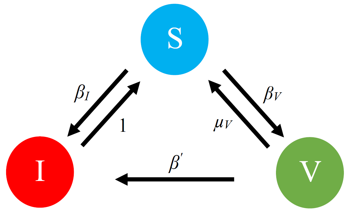
Figure 1: Schematic representation of dynamics of the model. The rates indicated are for the transition of a single individual. Transitions from I to S and V to S are spontaneous. The other three possible transitions occur through direct contacts between the individual changing state and a neighbor inducing the transition.

Let us denote the fractions of susceptible, infected, and vaccinated nodes with $x$, $y$, and $z$, respectively. Since the number of nodes, $N$, is constant, there is a conservation rule as $x+y+z=1$, and so $\dot{x}+\dot{y}+\dot{z}=0$.

According to the dynamics of the model, we can write down the following mean-field (MF) equations, which correspond to assuming that, at each time, each node interacts with a single other node selected randomly:

$$\dot{x} = -\beta_{V}x(1-x-y)-\beta_{I}xy+\mu_{V}(1-x-y)+y,~{}~{}~{}~{}$$ (1)

$$\dot{y} = \beta^{\prime}y(1-x-y)+\beta_{I}xy-y.~{}~{}~{}~{}\!\!\!\!\!$$ (2)

The first term on the right-hand side of Eq. (1) corresponds to the vaccination process ̵‌and accounts for the conversion of susceptible nodes into vaccinated ones with rate $\beta_{V}$, while the second term describes the infection process with the conversion of susceptible nodes into infected ones at rate $\beta_{I}$. The third and fourth terms account for the recovery from the vaccinated and infected state back to the susceptible state, occurring with rates $\mu_{V}$ and $1$, respectively. Similarly, the first term on the right hand side of Eq. (2) corresponds to the infection of vaccinated nodes (rate $\beta^{\prime}$). The second and third terms of Eq. (2) correspond to the conversion of susceptible nodes into infected and $vice$ $versa$ according to the rules of the standard SIS dynamics.

To analyze stationary solutions of these equations, we determine the fixed points of the system. Imposing $\dot{x}=\dot{y}=0$ leads to the following fixed points:

$$(1)\rightarrow ~{}~{}(x_{1}^{*},y_{1}^{*},z_{1}^{*})= (1,0,0),$$ (3)

$$(2)\rightarrow ~{}~{}(x_{2}^{*},y_{2}^{*},z_{2}^{*})= \left(\frac{\mu_{V}}{\beta_{V}},0,1-\frac{\mu_{V}}{\beta_{V}}\right),~{}~{}~{}$$ (4)

$$(3)\rightarrow ~{}~{}(x_{3}^{*},y_{3}^{*},z_{3}^{*})= \left(\frac{1}{\beta_{I}},1-\frac{1}{\beta_{I}},0\right),~{}~{}~{}$$ (5)

$$(4)\rightarrow ~{}~{}(x_{4}^{*},y_{4}^{*},z_{4}^{*})= \bigg{(}\frac{\mu_{V}+\beta^{\prime}-1}{\beta^{\prime}-\beta_{I}+\beta_{V}},~{}~{}~{}$$ (6)

$$\frac{\mu_{V}(\beta_{I}-\beta^{\prime})+\beta_{V}\left({\beta^{\prime}-1}\right)}{\beta^{\prime}\left({\beta^{\prime}-\beta_{I}+\beta_{V}}\right)},~{}~{}~{}$$

$$\frac{\beta^{\prime}(1-\beta_{I})+\beta_{V}-\mu_{V}\beta_{I}}{\beta^{\prime}(\beta^{\prime}-\beta_{I}+\beta_{V})}\bigg{)}.$$

The trivial fixed point 1 indicates the state in which all nodes are susceptible, i.e., the absorbing state. Fixed point 2 corresponds to a state in which there are no infected nodes, while there is a coexistence of susceptible and vaccinated ones (“disease-free immunized” state). Fixed point 3 is perfectly analogous to fixed point 2 but now the coexistence is between susceptible and infected nodes: it is the usual active state of SIS dynamics (“vaccinated-free epidemic” state). Finally fixed point 4 corresponds to a state in which the fraction of susceptible, infected, and vaccinated nodes are all different from zero (“mixed” state). The relevance of these fixed points for the SIV dynamics depends on their stability and whether their coordinates are physical, i.e., within the range between 0 and 1. By stability we intend that the stationary solutions must be deterministically stable in the limit of infinite size. The Jacobian matrix associated to the MF equations (1) and (2) is

The analysis is made easier by first distinguishing between the cases $\beta_{V}/\mu_{V}<1$ and $\beta_{V}/\mu_{V}>1$. They correspond, respectively, to the inactive and the active phase of the SIS dynamics for the vaccination process (alone) in mean-field. In other words for $\beta_{V}/\mu_{V}<1$ the vaccination rate is insufficient to sustain the presence of a finite fraction of vaccinated individuals in the system. Even neglecting the possibility of V $\to$ I transitions, the density of vaccinated nodes decreases and tends to zero spontaneously. It is then reasonable to expect that the stationary state of the overall system will be exactly the same of a normal SIS process for disease spreading. In the case $\beta_{V}/\mu_{V}>1$ instead, the vaccination process in isolation would lead to a finite prevalence of vaccinated nodes. It is then interesting (and nontrivial) to investigate how this interplays with the disease spreading process.

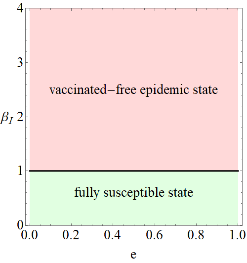
Figure 2: Phase diagram of the model for $\beta_{V}/\mu_{V}<1$ as a function of $\beta_{I}$ and $e$. The solid line shows the continuous transition at $\beta_{I}=1$.

II.1 The case $\frac{\beta_{V}}{\mu_{V}}<1$

In this case, the fixed point 2 is not physical (as $x_{2}^{*}>1$), so only three fixed points are relevant.

II.1.1 Stability of fixed point 1

The Jacobian matrix of the system for the first fixed point has eigenvalues:

$$\left\{\begin{array}[]{l}{\lambda_{1}}=\beta_{V}-\mu_{V},\\ {\lambda_{2}}=\beta_{I}-1.\end{array}\right.$$ (8)

In this regime, $\lambda_{1}$ is negative. Hence, in order for the fixed point 1 to be stable, the infection rate $\beta_{I}$ must be smaller than 1.

II.1.2 Stability of fixed point 3

The Jacobian matrix evaluated at the third fixed point has the following eigenvalues:

$$\left\{\begin{array}[]{l}{\lambda_{1}}=1-\beta_{I},\\ {\lambda_{2}}=\frac{{\beta_{V}+\beta^{\prime}-\mu_{V}\beta_{I}-\beta_{I}\beta^{\prime}}}{\beta_{I}}.\end{array}\right.$$ (9)

The first eigenvalue is negative if $\beta_{I}>1$. The condition for the second to be negative is

$$\beta_{I}>\frac{\beta_{V}+\beta^{\prime}}{\mu_{V}+\beta^{\prime}}=1+\frac{\beta_{V}-\mu_{V}}{\beta^{\prime}+\mu_{V}}.$$ (10)

Since $\beta_{V}<\mu_{V}$, for $\beta_{I}>1$ both eigenvalues are negative and the fixed point is stable.

II.1.3 Stability of fixed point 4

The eigenvalues of the Jacobian matrix for the fourth fixed point are:

$$\left\{\begin{array}[]{l}{\lambda_{1}}=\frac{{(\mu_{V}\beta_{I}-\beta_{V})-\sqrt{\frac{X}{{-F}}}}}{{2\beta^{\prime}}},\\ {\lambda_{2}}=\frac{{(\mu_{V}\beta_{I}-\beta_{V})+\sqrt{\frac{X}{{-F}}}}}{{2\beta^{\prime}}}.\end{array}\right.$$ (11)

where,

$$X=4A\beta^{\prime 3}+4B\beta^{\prime 2}+5C\beta^{\prime}+D,$$ (12)

$$A=(\mu_{V}-\beta_{V})(\beta_{I}-1),$$

$$B=(\mu_{V}\beta_{I}-\beta_{V})((1-\beta_{I})+(\mu_{V}-\beta_{V})),$$

$$C=-{(\mu_{V}\beta_{I}-\beta_{V})^{2}},$$

$$D=(\mu_{V}\beta_{I}-\beta_{V})^{2}(\beta_{I}-\beta_{V}),$$

$$F=\beta_{V}+\beta^{\prime}-\beta_{I}.$$

In order for the real part of both eigenvalues to be negative, a necessary condition is ${(\mu_{V}\beta_{I}-\beta_{V})}<0$ (independent of the value of $\sqrt{\frac{X}{-F}}$). This condition means that $\beta_{I}<\frac{\beta_{V}}{\mu_{V}}$. If this condition is satisfied, the real part of $\lambda_{1}$ is necessarily negative. The real part of $\lambda_{2}$ is negative as well if $\frac{X}{{-F}}<(\mu_{V}\beta_{I}-\beta_{V})^{2}$. Whether this condition is fulfilled it depends on the sign of $F$. For $F>0$, the condition is satisfied if $X>-F(\mu_{V}\beta_{I}-\beta_{V})^{2}$, which corresponds to an inequality of the following general form:

$$A{{\beta^{\prime}}^{2}}+B\beta^{\prime}+C>0.$$ (13)

Since $\beta_{V}<\mu_{V}$, all coefficients $A$, $B$, and $C$ are negative [Eqs. (12)]. Hence, the inequality (13) is not satisfied for positive values of $\beta^{\prime}$. Therefore, the fourth fixed point is never stable if $F>0$. Instead for $F<0$, the sign of Eq. (13) is reversed, and the inequality is always satisfied. From the conditions $\beta_{I}<\frac{\beta_{V}}{\mu_{V}}$ and $F<0$ we obtain that the fourth fixed point is stable in the interval $\frac{\beta_{V}}{e}<\beta_{I}<\frac{\beta_{V}}{\mu_{V}}$. In this interval we must check also that $x_{4}^{*}$, $y_{4}^{*}$, and $z_{4}^{*}$ belong to the interval $(0,1)$. It can be proved that for all values of $e$, $x_{4}^{*}$, and $y_{4}^{*}$ are never simultaneously physical (see Appendix A). In summary, in the case $\beta_{V}<\mu_{V}$, the fourth fixed point is never stable and physical at the same time.

We can conclude that, if $\beta_{I}<1$, the fixed point 1 (fully susceptible state) is stable, while if $\beta_{I}>1$, the fixed point 3 (vaccinated-free epidemic state) is stable. Therefore, as expected, in this regime the phase diagram is the same of the standard SIS model for the spreading of a single disease (Fig. 2). The presence of vaccinated individuals has effects only in the transient time before the stationary state.

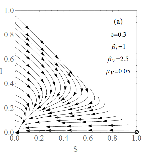
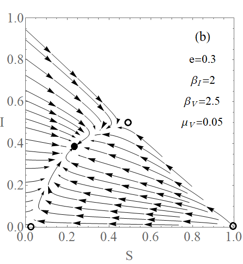
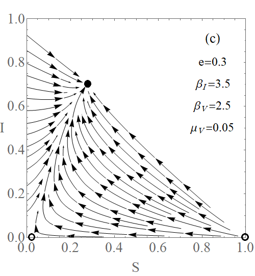
Figure 3: Phase portraits for $e<e_{c}$ and $(a)$ $\beta_{I}<\beta_{V}^{*}$, $(b)$ $\beta_{V}^{*}<\beta_{I}<\beta_{E}^{*}$, and $(c)$ $\beta_{I}>\beta_{E}^{*}$. For the chosen values of $\beta_{V}$, $\mu_{V}$, and $e$, we find $\beta_{V}^{*}\simeq 1.416$, $\beta_{E}^{*}\simeq 2.410$, and $e_{c}\simeq 0.724$. Solid black dots represent stable fixed points, and open circles show saddle or unstable fixed points.

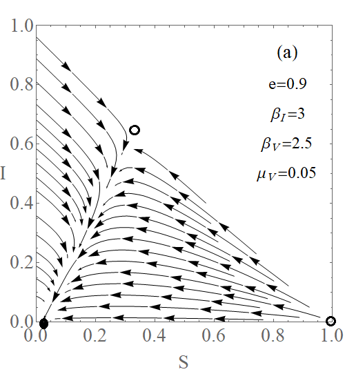
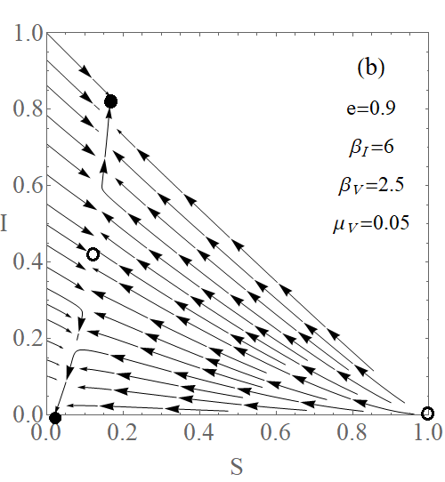
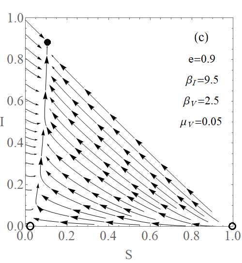
Figure 4: Phase portraits for $e>e_{c}$, $(a)$ $\beta_{I}<\beta_{E}^{*}$, $(b)$ $\beta_{E}^{*}<\beta_{I}<\beta_{V}^{*}$, and $(c)$ $\beta_{I}>\beta_{V}^{*}$. For the chosen values of $\beta_{V}$, $\mu_{V}$, and $e$, we find $\beta_{V}^{*}\simeq 8.474$, $\beta_{E}^{*}\simeq 5.256$, and $e_{c}\simeq 0.724$. Solid black dots represent stable fixed points and open circles show saddle or unstable fixed points.

II.2 The case $\frac{\beta_{V}}{\mu_{V}}>1$

II.2.1 Stability of fixed point 1

The eigenvalues of the Jacobian matrix for this fixed point are given by Eq. (8). In this regime $\lambda_{1}$ is always positive, hence this fixed point, which is a saddle node for $\beta_{I}<1$ ($\lambda_{2}<0$), is never stable.

II.2.2 Stability of fixed point 2

The Jacobian matrix of the system for the second fixed point has eigenvalues:

$$\left\{{\begin{array}[]{*{20}{l}}{{\lambda_{1}}=\mu_{V}-\beta_{V}},\\ {{\lambda_{2}}=\frac{{-\beta_{V}-\mu_{V}\beta^{\prime}+\mu_{V}\beta_{I}+\beta_{V}\beta^{\prime}}}{\beta_{V}}}\end{array},}\right.$$ (14)

$\lambda_{1}$ is always negative. Hence, the fixed point is stable if $\lambda_{2}<0$, which requires:

$$\beta_{I}<\frac{\beta_{V}}{\beta_{V}(1-e)+e\mu_{V}}\equiv\beta_{V}^{*}.$$ (15)

II.2.3 Stability of fixed point 3

The eigenvalues of the Jacobian matrix evaluated for the third fixed point are given by Eq. (9). This fixed point is physical for $\beta_{I}>1$, a condition that guarantees that $\lambda_{1}<0$. For having $\lambda_{2}<0$, the inequality $\beta_{I}>\frac{{\beta_{V}+\beta^{\prime}}}{{\mu_{V}+\beta^{\prime}}}$ must hold. By substituting $\beta^{\prime}=\beta_{I}(1-e)$, we obtain the following inequality for $\beta_{I}$:

$$f(\beta_{I})\equiv{\beta_{I}^{2}}(1-e)+\beta_{I}(\mu_{V}+e-1)-\beta_{V}>0.$$ (16)

This inequality is satisfied for $\beta_{I}>\beta_{E}^{*}$, where $\beta_{E}^{*}$ is the positive root of $f(\beta_{I})=0$:

$$\beta_{E}^{*}\equiv\frac{(1-\mu_{V}-e)+\sqrt{(\mu_{V}+e-1)^{2}+4\beta_{V}(1-e)}}{2(1-e)}.$$ (17)

Therefore, the third fixed point is stable for $\beta_{I}>\beta_{E}^{*}$.

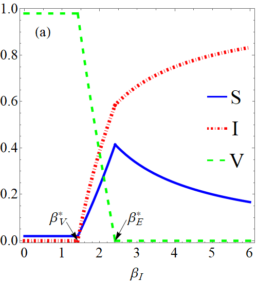
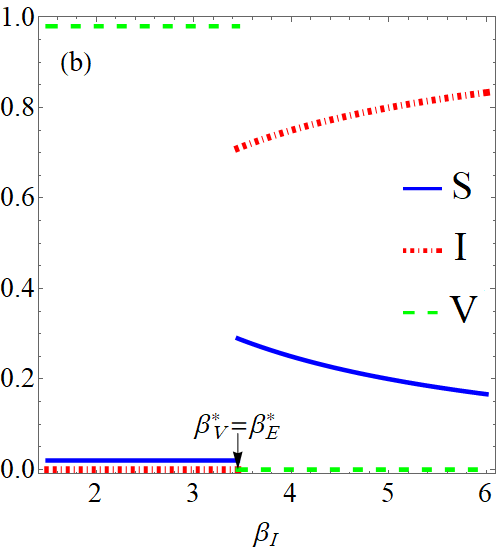
Figure 5: Stationary values of the fraction of susceptible, infected, and vaccinated nodes as a function of $\beta_{I}$ for $\beta_{V}=2.5$ and $\mu_{V}=0.05$ ($e_{c}\simeq 0.724$). The vaccine efficiency is set to $(a)$ $e=0.3$, $(b)$ $e=e_{c}$, and $(c)$ $e=0.9$.

II.2.4 Stability of fixed point 4

As discussed in Sec. II.1.3, one condition for stability of this fixed point is $\beta_{I}<\frac{\beta_{V}}{\mu_{V}}$. In order to discuss the other conditions we separate again the cases $F>0$ and $F<0$. Let us define the threshold value $e_{c}$ for the vaccine efficiency (see Appendix A):

$${e_{c}}\equiv\frac{\beta_{V}}{{1+\beta_{V}-\mu_{V}}}.$$ (18)

For $F>0$, if $e>e_{c}$ the fixed point 4 cannot be stable, while if $e<e_{c}$, this fixed point is stable and physical in the interval $\beta_{V}^{*}<\beta_{I}<\beta_{E}^{*}$ (see Appendix B). However, for $F<0$, it can be shown that neither for $e>e_{c}$ nor for $e<e_{c}$ the fixed point is both physical and stable (see Appendix C). Furthermore, in Appendix D we prove that for $e<e_{c}$ the parameter $\beta_{V}^{*}$ is smaller than $\beta_{E}^{*}$ while for $e>e_{c}$ the opposite is true.

We can summarize the stability of the fixed points for the case $\beta_{V}/\mu_{V}>1$ as follows:

1. If $e<e_{c}$, then $\beta_{V}^{*}<\beta_{E}^{*}$, and

   1. For $\beta_{I}<\beta_{V}^{*}$, only fixed point 2 is stable.

   2. For $\beta_{V}^{*}<\beta_{I}<\beta_{E}^{*}$, only fixed point 4 is stable.

   3. For $\beta_{I}>\beta_{E}^{*}$, only fixed point 3 is stable.

2. If $e>e_{c}$, then $\beta_{E}^{*}<\beta_{V}^{*}$, and

   1. For $\beta_{I}<\beta_{E}^{*}$, only fixed point 2 is stable.

   2. For $\beta_{E}^{*}<\beta_{I}<\beta_{V}^{*}$, both fixed points 2 and 3 are stable.

   3. For $\beta_{I}>\beta_{V}^{*}$, only fixed point 3 is stable.

These results are confirmed in Figs. 3 and 4 for two values of vaccine efficiency below and above the threshold value $e_{c}$. The stable fixed points are represented by black solid dots in the phase space $(S,I)$. Figure 3 is plotted for $e=0.3<e_{c}\simeq 0.724$. We change the value of $\beta_{I}$ such that in Fig. 3(a) the fixed point 2 is stable, and in Figs. 3(b) and  3(c) the fixed points 4 and 3 are stable, respectively. Similarly, for $e=0.9>e_{c}$, Fig. 4 shows the interval of values of $\beta_{I}$ for which one or both fixed point 2 or 3 are stable.

The fractions of susceptible (S), infected (I), and vaccinated (V) nodes are plotted as a function of $\beta_{I}$ in Fig. 5. Figure 5(a) shows the case $e<e_{c}$. In this case when $\beta_{I}<\beta_{V}^{*}$, we have a disease-free immunized state and only the fixed point 2 is stable, i.e., some nodes are susceptible and the others are vaccinated. Increasing the value of $\beta_{I}$, a continuous transition occurs (fixed point 4 becomes stable), and for $\beta_{V}^{*}<\beta_{I}<\beta_{E}^{*}$ a finite fraction of infected nodes is present in the stationary state. As we increase $\beta_{I}$ further, above $\beta_{I}=\beta_{E}^{*}$, the fraction of vaccinated nodes becomes zero (fixed point 3 becomes stable). The transition to this vaccinated-free epidemic state is also continuous. When $e=e_{c}$ [Fig. 5(b)], the two transition points $\beta_{V}^{*}$ and $\beta_{E}^{*}$ coincide, and a discontinuous transition occurs from the disease-free immunized state to the vaccinated-free epidemic state. In other words, at $e=e_{c}$ the type of the transitions is changed from continuous to discontinuous and the model exhibits a tricritical point. For the values we consider, $\beta_{V}=2.5$ and $\mu_{V}=0.05$, the tricritical point occurs at $(e_{c},\beta_{Ic})=(0.724,3.45)$. For $e>e_{c}$ [Fig. 5(c)], the value of $\beta_{E}^{*}$ is smaller than $\beta_{V}^{*}$. So, in the interval $\beta_{E}^{*}<\beta_{I}<\beta_{V}^{*}$, both the disease-free immunized and vaccinated-free epidemic states are possible (both fixed points 2 and 3 are stable) and bistability emerges. Notice that for $\mu_{V}>1$, $e_{c}$ is larger than 1 and we always have $e<e_{c}$. Hence the bistability emerges only for values $\mu_{V}<1$. We can see the full phase diagram of the model for the case $\beta_{V}>\mu_{V}$ in Fig. 6.

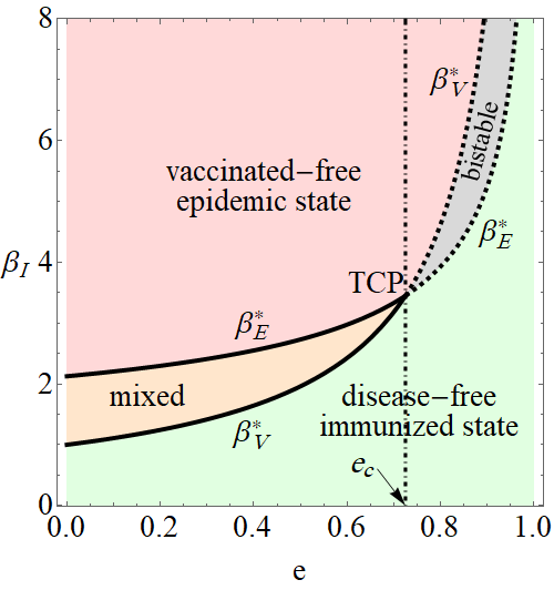
Figure 6: Phase diagram of the model for $\beta_{V}/\mu_{V}>1$ ($\beta_{V}=2.5$ , $\mu_{V}=0.05$) as a function of $\beta_{I}$ and $e$. The solid lines show continuous while dashed curves indicate the discontinuous transition points. The tricritical point is located at $(e_{c},\beta_{Ic})=(0.724,3.45)$. The transition lines are computed from Eqs. (15) and (17).

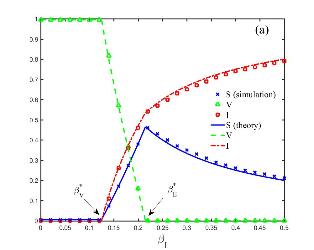
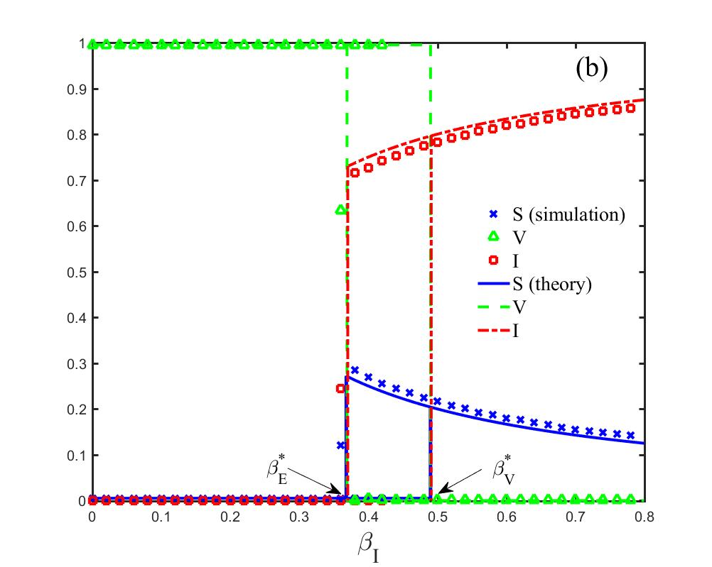
Figure 7: Stationary values for susceptible (S), infected (I), and vaccinated (V) densities versus the infection rate $\beta_{I}$ on the $ER$ network with $\langle k\rangle=10$. Symbols show the results of numerical simulations, which are in agreement with the mean-field approach (solid lines). In both panels $\beta_{V}=0.2$ and $\mu_{V}=0.01$ ($e_{c}\simeq 0.668$). In $(a)$ the vaccine efficiency is set to $e=0.2<e_{c}$, and the initial condition of the simulations is $I_{0}=0.1$, $V_{0}=0.9$. Transition points are $\beta_{V}^{*}\simeq 0.124$ and $\beta_{E}^{*}\simeq 0.215$. In panel $(b)$ $e=0.8>e_{c}$ and for the forward diagram $I_{0}=0.1$,$V_{0}=0.01$, while for the backward diagram $I_{0}=0.01$ and $V_{0}=0.99$. Transition points are $\beta_{E}^{*}\simeq 0.367$ and $\beta_{V}^{*}\simeq 0.490$.

II.3 The case of perfect vaccination $e=1$

An interesting special case of the general framework presented above occurs when the vaccination is fully effective ($e=1$, i.e., $\beta^{\prime}=0$) so that the direct transition $V\to I$ is prohibited. In this case there is a perfect symmetry between the two competing SIS processes, which is not apparent only because we have set $\mu_{I}=1$ from the outset, while we have kept $\mu_{V}$ free. In this case only the first three fixed points are present: Fixed point 4 disappears for $\beta^{\prime}=0$. The fixed point 1 is stable if both $\beta_{I}<1$ and $\beta_{V}/\mu_{V}<1$. In such a case both SIS processes spontaneously vanish and the absorbing, fully susceptible state, is reached. The other two possible stationary states are fixed point 2 (disease-free immunized state), which is reached if $\beta_{V}/\mu_{V}>1$ and $\beta_{V}/\mu_{V}>\beta_{I}$, and fixed point 3 (vaccinated-free epidemic state) reached if $\beta_{I}>1$ and $\beta_{I}>\beta_{V}/\mu_{V}$. We conclude that, in the perfectly symmetric case, only the most infective SIS process can asymptotically survive, leading to the complete eradication of the other. A mixed state with coexistence of I and V individuals in the stationary state is possible only in the presence of an imperfect vaccination, i.e., an asymmetry between the two competing processes.

III Numerical Simulations on homogeneous networks

So far we have considered the mean-field solution of the SIV model, corresponding to its behavior in the case a node interacts with a single random neighbor. A more realistic case is to consider the model on structured networks. Let us consider the Erdős–Rényi (ER) random network with mean degree $\langle k\rangle$, a paradigmatic example of a homogeneous network. To describe this system the mean-field equations must be modified, to take into account that each node is in contact, on average, with $\langle k\rangle$ other nodes. Hence the equations are exactly the same provided all transmission rates ($\beta_{I},\beta_{V},\beta^{\prime}$) are multiplied by the factor $\langle k\rangle$. Substituting these values into Eqs. (1) and (2), the fixed points of the model are now

$$(1)\rightarrow ~{}~{}(x_{1}^{*},y_{1}^{*},z_{1}^{*})= (1,0,0),$$ (19)

$$(2)\rightarrow ~{}~{}(x_{2}^{*},y_{2}^{*},z_{2}^{*})= \left(\frac{\mu_{V}}{\langle k\rangle\beta_{V}},0,1-\frac{\mu_{V}}{\langle k\rangle\beta_{V}}\right),~{}~{}~{}$$ (20)

$$(3)\rightarrow ~{}~{}(x_{3}^{*},y_{3}^{*},z_{3}^{*})= \left(\frac{1}{\langle k\rangle\beta_{I}},1-\frac{1}{\langle k\rangle\beta_{I}},0\right),~{}~{}~{}$$ (21)

$$(4)\rightarrow ~{}~{}(x_{4}^{*},y_{4}^{*},z_{4}^{*})= \bigg{(}\frac{\mu_{V}+\langle k\rangle\beta^{\prime}-1}{\langle k\rangle(\beta^{\prime}-\beta_{I}+\beta_{V})},~{}~{}~{}$$ (22)

$$\frac{\mu_{V}(\beta_{I}-\beta^{\prime})+\beta_{V}\left({\langle k\rangle\beta^{\prime}-1}\right)}{\langle k\rangle\beta^{\prime}\left({\beta^{\prime}-\beta_{I}+\beta_{V}}\right)},~{}~{}~{}$$

$$\frac{\beta^{\prime}(1-\langle k\rangle\beta_{I})+\beta_{V}-\mu_{V}\beta_{I}}{\langle k\rangle\beta^{\prime}(\beta^{\prime}-\beta_{I}+\beta_{V})}\bigg{)}.$$

All the arguments in the previous section extend to this case, provided the threshold $e_{c}$ and the transition points $\beta_{V}^{*}$ and $\beta_{E}^{*}$ are redefined as follows:

$$e_{c} = \frac{\langle k\rangle\beta_{V}}{{1+\langle k\rangle\beta_{V}-\mu_{V}}},$$ (23)

$$\beta_{V}^{*} = \frac{\beta_{V}}{\langle k\rangle\beta_{V}(1-e)+e\mu_{V}},$$ (24)

$$\beta_{E}^{*} = \frac{(1-\mu_{V}-e)+\sqrt{(\mu_{V}+e-1)^{2}+4\langle k\rangle\beta_{V}(1-e)}}{2(1-e)\langle k\rangle}.$$

As we can see from Eq. (23), the critical value of vaccine efficiency depends on the connectivity $\left\langle{k}\right\rangle$ of the network. When the connectivity is increased, $e_{c}$ approaches 1 and so the region of bistability tends to disappear. This observation can be rationalized as follows. For a strongly leaky vaccine, $e<e_{c}$, a mixed state arises due to the presence of a loop of transitions ($S\to V\to I\to S$), in a way analogous to the rock-paper-scissors dynamics Szolnoki et al. (2014). Bistability is observed only when the $V\to I$ process in this loop is suppressed, which happens when $\beta^{\prime}$ is sufficiently small (i.e., the vaccine efficiency is larger than the critical value $e_{c}$). Increasing $\left\langle{k}\right\rangle$ implies that vaccinated individuals have more infected neighbors and so their chance of getting infected is increased: in other words, the process $V\to I$ is enhanced. In order to see bistability one needs $\beta^{\prime}$ to be reduced to compensate for the increase of connectivity. This explains why $e_{c}$ grows with $\left\langle{k}\right\rangle$ and bistability tends to disappear as connectivity becomes large.

To validate the analytical results, we perform (using a continuous time Gillespie algorithm), numerical simulations of the SIV dynamics on ER random networks. We consider a network consisting of $N=10^{4}$ nodes and with mean degree $\langle k\rangle=10$ and select parameters of the model corresponding to the two cases $e<e_{c}$ and $e>e_{c}$. Let us set $\beta_{V}=0.2$ and $\mu_{V}=0.01$, so that $\beta_{V}/\mu_{V}>1$. According to Eq. (LABEL:eq16), the efficiency threshold is $e_{c}\simeq 0.668$. We first consider the value $e=0.2<e_{c}$ so that we expect the presence of a mixed state. We choose the initial conditions as $I_{0}=0.1$, $V_{0}=0.9$ and $S_{0}=0$ and average over 20 realizations. Figure. 7(a) shows the stationary values for the fractions of susceptible, infected, and vaccinated nodes as a function of the infection rate $\beta_{I}$. We can see that numerical simulations (symbols) are in good agreement with analytical results (curves), obtained in the previous sections. In this case the transition points are $\beta_{V}^{*}\simeq 0.124$ and $\beta_{E}^{*}\simeq 0.215$ [Eq. (LABEL:eq16)], which are very close to the numerical results. Next we consider a vaccine efficiency $e=0.8>e_{c}$. In this case the dependence of the densities on $\beta_{I}$ is qualitatively different and a hysteresis loop appears [Fig. 7(b)]. For the initial condition $I_{0}=0.1$ and $V_{0}=0.01$ a discontinuous transition occurs for $\beta_{I}\simeq\beta_{V}^{*}\simeq 0.490$. If we choose the initial condition as $I_{0}=0.01$ and $V_{0}=0.99$, the transition point is instead $\beta_{I}\simeq\beta_{E}^{*}\simeq 0.367$.

IV Conclusions

In this work, we have studied a three-state SIV model in which disease spreading competes with a vaccination process. We have assumed both disease and vaccination spreading follow the dynamics of the standard SIS model. Hence, similar to the disease, the vaccination is also considered as a contact process such that vaccinated individuals convince their susceptible neighbors to be vaccinated. We have assumed an imperfect vaccination so that vaccinated individuals can be infected at a reduced rate. This couples asymmetrically the two competing models.

We have identified the existence of two completely different scenarios. If the vaccination rate is not large enough with respect to the rate at which immunity fades away, the vaccination process does not have any effect on disease spreading in the stationary state and the same phase diagram of the standard SIS model is obtained. Instead, if the vaccination is large enough new “disease-free immunized” and “mixed” phases appear. For a small value of vaccine efficiency, the model shows two continuous transitions as the infection rate is increased. The first transition occurs from the disease-free immunized phase, in which only susceptible and vaccinated nodes exist, to the mixed phase with a mixture of susceptible, infected, and vaccinated nodes. The second transition occurs at a higher infection rate and separates the mixed phase from the vaccinated-free epidemic phase, in which no vaccinated nodes are present. For larger vaccine efficiency, above a tricritical point, the mixed phase disappears and is replaced by a bistability region, with both disease-free immunized and vaccinated-free epidemic states stable.

We have checked that the MF scenario depicted above is observed also when the interaction pattern is described by a homogeneous network. Whether this remains true also for more complex topologies (such as heterogeneous, clustered, or correlated networks) is a promising avenue for future research. Another path that could be followed is the investigation of the role of the imperfect vaccination. Its presence creates an asymmetric direct coupling between V and I states, that induces the possibility of cyclic transitions in the model. It would be interesting to analyze the similarities and differences with respect to other cyclical competing three-state dynamics, such as the rock-paper-scissors model.

Appendix A

For $F=\beta_{V}+\beta^{\prime}-\beta_{I}<0$, from the physical condition $0<x_{4}^{*}<1$ we obtain that $\beta_{I}$ must be less than $\frac{1-\mu_{V}}{1-e}$ and greater than $1+\beta_{V}-\mu_{V}$. An overlap interval exists if the following subtraction is positive:

$$\frac{1-\mu_{V}}{1-e}-(1+\beta_{V}-\mu_{V})=\frac{e-\beta_{V}+e\beta_{V}-e\mu_{V}}{1-e}.$$ (26)

Let us define a threshold value for efficiency of vaccination as follows:

$${e_{c}}\equiv\frac{\beta_{V}}{{1+\beta_{V}-\mu_{V}}}.$$ (27)

The relation (26) is positive if $e>e_{c}$. In this case the physical condition for $x_{4}^{*}$ is satisfied. On the other hand, from $y_{4}^{*}>0$ it is concluded that $\beta_{I}$ also must be less than $\frac{\beta_{V}}{\beta_{V}(1-e)+e\mu_{V}}\equiv\beta_{V}^{*}$. That means $\beta_{V}^{*}$ must be greater than $1+\beta_{V}-\mu_{V}$ or the following subtraction must be negative:

$$(1+\beta_{V}-\mu_{V})-\beta_{V}^{*}=(1+\beta_{V}-\mu_{V})$$ (28)

$$-\frac{\beta_{V}}{\beta_{V}(1-e)+e\mu_{V}}$$

$$=\frac{(e-\beta_{V}+e\beta_{V}-e\mu_{V})(\mu_{V}-\beta_{V})}{\beta_{V}(1-e)+e\mu_{V}}.$$

For $e>e_{c}$, we have $(e+e\beta_{V}-e\mu_{V}-\beta_{V})>0$, and since $\mu_{V}>\beta_{V}$, the subtraction is always positive. Hence the physical conditions for $x_{4}^{*}$ and $y_{4}^{*}$ are not satisfied simultaneously.

Appendix B

For $F>0$, as we discussed in Subsec. (II.1.3), the stability condition for the fourth fixed point leads to Eq. (13). If one substitutes $\beta^{\prime}=\beta_{I}(1-e)$, Eq. (13) can be rewritten as an inequation of order 3 for $\beta_{I}$:

$$g(\beta_{I})\equiv a\beta_{I}^{3}+b\beta_{I}^{2}+c\beta_{I}+d>0,$$ (29)

where

$$a=-(1-e)\left(e\mu_{V}+\beta_{V}(1-e)\right)<0$$ (30)

and $b$, $c$, and $d$ are some parameters. $g(\beta_{I})=0$ has three roots:

$${\beta_{I1}}=\frac{{(1-\mu_{V}-e)+\sqrt{{{(\mu_{V}+e-1)}^{2}}+4\beta_{V}(1-e)}}}{{2(1-e)}}\equiv\beta_{E}^{*},$$ (31)

$${\beta_{I2}}=\frac{{(1-\mu_{V}-e)-\sqrt{{{(\mu_{V}+e-1)}^{2}}+4\beta_{V}(1-e)}}}{{2(1-e)}},$$ (32)

$${\beta_{I3}}=\frac{\beta_{V}}{{\beta_{V}(1-e)+e\mu_{V}}}\equiv\beta_{V}^{*},$$ (33)

such that $\beta_{E}^{*}$ and $\beta_{V}^{*}$ are positive but $\beta_{I2}$ is negative. Since the coefficient of cubic term (parameter $a$) is always negative, we conclude that the inequality (29) is satisfied for $\beta_{I}$ between positive roots $\beta_{E}^{*}$ and $\beta_{V}^{*}$. On the other hand, $\beta_{I}$ must satisfy the two additional conditions $\beta_{I}<\frac{\beta_{V}}{\mu_{V}}$ and $\beta_{I}<\frac{\beta_{V}}{e}$. Let us consider two cases:

1. $e>e_{c}$: According to Appendix F, both $\beta_{E}^{*}$ and $\beta_{V}^{*}$ are greater than $\frac{\beta_{V}}{e}$, Hence the condition $\beta_{I}<\frac{\beta_{V}}{e}$ is not satisfied.

2. $e<e_{c}$: In this case, $\beta_{V}^{*}$ is less than $\beta_{E}^{*}$ (see Appendix D), and both are less than $\frac{\beta_{V}}{\mu_{V}}$ and $\frac{\beta_{V}}{e}$ as proved in Appendixes E and F, respectively.

Hence, the fourth fixed point is stable in the interval $\beta_{V}^{*}<\beta_{I}<\beta_{E}^{*}$ when $e<e_{c}$ and $F>0$. Now, we must check the following six physical conditions:

1. $x_{4}^{*}>0\to\beta_{I}>\frac{1-\mu_{V}}{1-e}$

2. $x_{4}^{*}<1\to\beta_{I}<1+\beta_{V}-\mu_{V}$

3. $y_{4}^{*}>0\to\beta_{I}>\beta_{V}^{*}$

4. $y_{4}^{*}<1\to\beta_{I}<\beta_{c1}\\ \beta_{c1}\equiv\frac{-e\mu_{V}+\sqrt{e^{2}\mu_{V}^{2}+4\beta_{V}e(1-e)}}{2e(1-e)}$

5. $z_{4}^{*}>0\to\beta_{I}<\beta_{E}^{*}$

6. $z_{4}^{*}<1\to\beta_{I}>\beta_{c2}\\ \leavevmode\resizebox{385.20253pt}{}{$\beta_{c2}\equiv\frac{{(1-\beta_{V})(1-e)-\mu_{V}+\sqrt{{((1-\beta_{V})(1-e)-\mu_{V})^{2}}+4\beta_{V}(1-e)^{2}}}}{{2(1-e)^{2}}}$ }$

Let us specify whether they can be satisfied or not, one by one:

1. Subtracting $\frac{1-\mu_{V}}{1-e}$ from $\beta_{V}^{*}$ (Appendix G), we conclude $\beta_{V}^{*}$ is more than it, so the condition is satisfied.

2. The result of subtracting $\beta_{E}^{*}$ from $(1+\beta_{V}-\mu_{V})$ is positive (Appendix H), hence this condition is true as well.

3. This one is clearly correct.

4. After some algebra, it is proved that for this state, $\beta_{E}^{*}$ is less than $\beta_{c1}$ (Appendix I), so this condition is also satisfied.

5. Obviously, that’s correct.

6. According to Appendix J, $\beta_{c2}<\beta_{V}^{*}$, so there is no problem with this condition too.

So far we conclude that the fourth fixed point is stable and physical for the interval $\beta_{V}^{*}<\beta_{I}<\beta_{E}^{*}$ when $e<e_{c}$.

Appendix C

If $F<0$ we must have $X<-F(\mu_{V}\beta_{I}-\beta_{V})^{2}$, such that the sign of Eq. (13) is reversed. Substituting $\beta^{\prime}=\beta_{I}(1-e)$, we obtain

$$g(\beta_{I})\equiv a\beta_{I}^{3}+b\beta_{I}^{2}+c\beta_{I}+d<0$$ (34)

where $a$ is the same as (30). In addition, from $F<0$ and the condition $\beta_{I}<\frac{\beta_{V}}{\mu_{V}}$, we find that $\frac{\beta_{V}}{e}<\beta_{I}<\frac{\beta_{V}}{\mu_{V}}$, which results in $\mu_{V}<e<1$. Let us check both stability and physical conditions for the obtained interval in two cases:

1. $e<e_{c}$: According to Appendix F, both $\beta_{V}^{*}$ and $\beta_{E}^{*}$, are less than $\frac{\beta_{V}}{e}$. Then $g(\beta_{I})$ is always negative. Hence, the condition $g(\beta_{I})<0$ is satisfied. The condition $x_{4}^{*}>0$, leads to $\beta_{I}<\frac{1-\mu_{V}}{1-e}$. On the other hand, $\frac{1-\mu_{V}}{1-e}<\frac{\beta_{V}}{e}$. Therefore, stability and the physical condition are not satisfied at the same time.

2. $e>e_{c}$: In this case both $\beta_{V}^{*}$ and $\beta_{E}^{*}$ are greater than $\frac{\beta_{V}}{e}$. From Appendixes D and E, we have $\beta_{E}^{*}<\beta_{V}^{*}<\frac{\beta_{V}}{\mu_{V}}$. So, the fourth fixed point can be stable in the intervals $\frac{\beta_{V}}{e}<\beta_{I}<\beta_{E}^{*}$ and $\beta_{V}^{*}<\beta_{I}<\frac{\beta_{V}}{\mu_{V}}$. On the other hand, for $y_{4}^{*}>0$ we need $\beta_{I}<\beta_{V}^{*}$, and for $z_{4}^{*}>0$ we must have $\beta_{I}>\beta_{E}^{*}$, which obviously contradict obtained intervals. So the fourth fixed point is not physical in this case as well.

Appendix D

Let us assume that $\beta_{E}^{*}-\beta_{V}^{*}>0$. In this case we have the following inequality:

$$\frac{{(1-\mu_{V}-e)+\sqrt{{{(\mu_{V}+e-1)}^{2}}+4\beta_{V}(1-e)}}}{{2(1-e)}}$$

$$-\frac{\beta_{V}}{\beta_{V}(1-e)+e\mu_{V}}>0.$$ (35)

The denominator of inequality (35) is positive. Hence the numerator must be positive as well:

$$\sqrt{{{(\mu_{V}+e-1)}^{2}}+4\beta_{V}(1-e)}>$$

$$\frac{2\beta_{V}(1-e)}{\beta_{V}(1-e)+e\mu_{V}}-(1-e-\mu_{V}).$$ (36)

After some calculations, we obtain that

$$e^{2}(\beta_{V}-\mu_{V})(\beta_{V}-\mu_{V}+1)$$

$$-e(\beta_{V}-\mu_{V})(\beta_{V}-\mu_{V}+\beta_{V}+1)$$

$$+\beta_{V}(\beta_{V}-\mu_{V})>0.$$ (37)

Notice that for case $\beta_{V}>\mu_{V}$, the coefficient of $e^{2}$ and the third term are both positive. The discriminant of the related quadratic equation is $\Delta=(\beta_{V}-\mu_{V})^{2}(\mu_{V}-1)^{2}$, which is also positive. Therefore, there are two real roots, $e_{1}=\dfrac{\beta_{V}}{1+\beta_{V}-\mu_{V}}=e_{c}$ and $e_{2}=1$. These roots are both positive for the case $\beta_{V}>\mu_{V}$. Regarding to the value of $\mu_{V}$, there are two statuses:

1. If $\mu_{V}<1$, then $e_{1}<e_{2}$. In this case for $e<e_{c}$ we have $\beta_{E}^{*}>\beta_{V}^{*}$, and for the opposite result is obtained for $e>e_{c}$.

2. If $\mu_{V}>1$, then $e_{1}>e_{2}$ and for each value of $e$, we have $\beta_{E}^{*}>\beta_{V}^{*}$. However, $e_{1}>e_{2}$ means that $e_{c}>1$, which never occurs since efficiency is always less than 1.

Appendix E

In order to compare $\beta_{V}^{*}$ and $\frac{\beta_{V}}{\mu_{V}}$, we discuss the sign of their difference:

$$\beta_{V}^{*}-\frac{\beta_{V}}{\mu_{V}}= \frac{\beta_{V}}{\beta_{V}(1-e)+e\mu_{V}}-\frac{\beta_{V}}{\mu_{V}}$$

$$= \frac{\beta_{V}(\mu_{V}-\beta_{V})(1-e)}{\mu_{V}(\beta_{V}(1-e)+e\mu_{V}))}.$$ (38)

If $\beta_{V}>\mu_{V}$, it is concluded that $\beta_{V}^{*}<\frac{\beta_{V}}{\mu_{V}}$ and in the opposite case $\beta_{V}<\mu_{V}$, we obtain the opposite result.

Similarly, we consider the subtraction $\beta_{E}^{*}-\frac{\beta_{V}}{\mu_{V}}$:

$$\beta_{E}^{*}-\frac{\beta_{V}}{\mu_{V}}=$$

$$\frac{{(1-\mu_{V}-e)+\sqrt{{{(\mu_{V}+e-1)}^{2}}+4\beta_{V}(1-e)}}}{{2(1-e)}}$$

$$-\frac{\beta_{V}}{\mu_{V}}.$$ (39)

Suppose that the result of this subtraction is negative. Since, the denominator is positive, it is concluded that

$$\mu_{V}\sqrt{{{(\mu_{V}+e-1)}^{2}}+4\beta_{V}(1-e)}<$$

$$2\beta_{V}(1-e)-\mu_{V}(1-e-\mu_{V}).$$ (40)

After some calculations, it is obtained that $(\beta_{V}-\mu_{V})(e-1)<0$, which is always correct for the case $\mu_{V}<\beta_{V}$. Therefore, we conclude that

1. If $\beta_{V}>\mu_{V}$, then $\beta_{E}^{*}<\frac{\beta_{V}}{\mu_{V}}$.

2. If $\beta_{V}<\mu_{V}$, then $\beta_{E}^{*}>\frac{\beta_{V}}{\mu_{V}}$.

Appendix F

Let us consider the following subtraction:

$$\beta_{V}^{*}-\frac{\beta_{V}}{e}= \frac{\beta_{V}}{\beta_{V}(1-e)+e\mu_{V}}-\frac{\beta_{V}}{e}$$

$$= \frac{\beta_{V}(e-e\mu_{V}-\beta_{V}+e\beta_{V})}{e(\beta_{V}(1-e)+e\mu_{V})}.$$ (41)

Since the denominator is positive, for $e>e_{c}$ we conclude that $(e+e\beta_{V}-e\mu_{V}-\beta_{V})>0$ and therefore $\beta_{V}^{*}>\frac{\beta_{V}}{e}$. In the same way for $e<e_{c}$, we obtain the opposite result, $\beta_{V}^{*}<\frac{\beta_{V}}{e}$.

Also we calculate the following subtraction:

$$\beta_{E}^{*}-\frac{\beta_{V}}{e}=$$

$$\frac{{(1-\mu_{V}-e)+\sqrt{{{(\mu_{V}+e-1)}^{2}}+4\beta_{V}(1-e)}}}{{2(1-e)}}-\frac{\beta_{V}}{e}$$

$$=\frac{{e(1-\mu_{V}-e)+e\sqrt{{{(\mu_{V}+e-1)}^{2}}+4\beta_{V}(1-e)}}}{{2e(1-e)}}$$

$$-\frac{2\beta_{V}(1-e)}{2e(1-e)}.$$ (42)

Let us assume that the result is positive. The denominator is positive, and therefore the nominator must be positive:

$$e\sqrt{{{(\mu_{V}+e-1)}^{2}}+4\beta_{V}(1-e)}>$$

$$2\beta_{V}(1-e)-e(1-e-\mu_{V}).$$ (43)

After some calculations, we obtain that $(e+e\beta_{V}-e\mu_{V}-\beta_{V})>0$, which leads to $e>e_{c}$. Consequently, for $e>e_{c}$ we get that $\beta_{E}^{*}>\frac{\beta_{V}}{e}$ and for $e<e_{c}$ the opposite result, namely, $\beta_{E}^{*}<\frac{\beta_{V}}{e}$, is obtained.

Appendix G

We can easily obtain that

$$\beta_{V}^{*}-\frac{1-\mu_{V}}{1-e}= \frac{\beta_{V}}{\beta_{V}(1-e)+e\mu_{V}}-\frac{1-\mu_{V}}{1-e}$$

$$= \frac{\mu_{V}(\beta_{V}-e-e\beta_{V}+e\mu_{V})}{(\beta_{V}(1-e)+e\mu_{V})(1-e)}.$$ (44)

Since the denominator is positive, in the case that $e>e_{c}$ we obtain $(e+e\beta_{V}-e\mu_{V}-\beta_{V})>0$. It results in

$$\beta_{V}^{*}<\frac{1-\mu_{V}}{1-e}.$$ (45)

With the same argument for $e<e_{c}$, the opposite result is obtained.

Also, we can see the difference between $\beta_{E}^{*}$ and $\frac{1-\mu_{V}}{1-e}$:

$$\beta_{E}^{*}-\frac{1-\mu_{V}}{1-e}=$$

$$\frac{{(1-\mu_{V}-e)+\sqrt{{{(\mu_{V}+e-1)}^{2}}+4\beta_{V}(1-e)}}}{{2(1-e)}}$$

$$-\frac{1-\mu_{V}}{1-e}.$$ (46)

If we assume that the result is negative, then since the denominator is positive we get

$$\sqrt{{{(\mu_{V}+e-1)}^{2}}+4\beta_{V}(1-e)}<1+e-\mu_{V}.$$ (47)

Hence, we conclude that $e+e\beta_{V}-e\alpha-\beta_{V}>0$, which is true for the case $e>e_{c}$. Therefore for $e>e_{c}$ it is obtained that $\beta_{E}^{*}<\frac{1-\mu_{V}}{1-e}$, and for the case $e<e_{c}$ the sign of inequality is opposite and $\beta_{E}^{*}$ is greater than $\frac{1-\mu_{V}}{1-e}$.

Appendix H

Next we consider the following subtraction:

$$\beta_{E}^{*}-(1+\beta_{V}-\mu_{V})=$$

$$\frac{{(1-\mu_{V}-e)+\sqrt{{{(\mu_{V}+e-1)}^{2}}+4\beta_{V}(1-e)}}}{{2(1-e)}}$$

$$-(1+\beta_{V}-\mu_{V}).$$ (48)

If the result is negative, since the denominator is positive we can write

$$\sqrt{{{(\mu_{V}+e-1)}^{2}}+4\beta_{V}(1-e)}<$$

$$e+\mu_{V}-1+2(1-e)(1+\beta_{V}-\mu_{V}).$$ (49)

Then $(\beta_{V}-\mu_{V})(\beta_{V}-e\beta_{V}+e\mu_{V}-e)>0$ if $\beta_{V}>\mu_{V}$ and $e<e_{c}$. Hence we can summarize the results as follows:

1. For $\beta_{V}>\mu_{V}$ :

   1. If $e<e_{c}$ then $\beta_{E}^{*}<(1+\beta_{V}-\mu_{V})$

   2. If $e>e_{c}$ then $\beta_{E}^{*}>(1+\beta_{V}-\mu_{V})$

2. For $\beta_{V}<\mu_{V}$ :

   1. If $e<e_{c}$ then $\beta_{E}^{*}>(1+\beta_{V}-\mu_{V})$

   2. If $e>e_{c}$ then $\beta_{E}^{*}<(1+\beta_{V}-\mu_{V})$

Appendix I

We assume that the following subtraction has positive sign:

$$\beta_{c1}-\beta_{E}^{*}=\frac{-e\mu_{V}+\sqrt{e^{2}\mu_{V}^{2}+4\beta_{V}e(1-e)}}{2e(1-e)}$$

$$-\frac{{(1-\mu_{V}-e)+\sqrt{{{(\mu_{V}+e-1)}^{2}}+4\beta_{V}(1-e)}}}{2(1-e)}>0.$$

The denominator is positive, hence we obtain $\frac{4\beta_{V}(1-e)(e\mu_{V}-e-e\beta_{V}+\beta_{V})}{e^{2}}>0$. This result is satisfied when $e<e_{c}$. Therefore, for $e>e_{c}$ we conclude that $\beta_{c1}<\beta_{E}^{*}$, while for $e<e_{c}$, the opposite result, namely, $\beta_{c1}>\beta_{E}^{*}$ is correct.

Appendix J

Let us assume that $\beta_{V}^{*}$ is greater than $\beta_{c2}$, such that the sign of following subtraction is positive:

$$\beta_{V}^{*}-\beta_{c2}=\frac{\beta_{V}}{\beta_{V}(1-e)+e\mu_{V}}$$

$$-\frac{{(1-\beta_{V})(1-e)-\mu_{V}}}{{2(1-e)^{2}}}$$

$$-\frac{\sqrt{{((1-\beta_{V})(1-e)-\mu_{V})^{2}}+4\beta_{V}(1-e)^{2}}}{2(1-e)^{2}}.$$ (51)

The denominator is positive, hence we can write:

$$-e(1-e)[(\mu_{V}-\beta_{V})^{2}+(\beta_{V}^{2}-\mu_{V})]-\mu_{V}\beta_{V}(1+e^{2})<0.$$

which is always correct for the case $\beta_{V}>\mu_{V}$. In other words if $\beta_{V}>\mu_{V}$, we have $\beta_{V}^{*}>\beta_{c2}$.

References

- Newman (2002) M. E. J. Newman, Phys. Rev. E 66, 016128 (2002).
- Pastor-Satorras et al. (2015) R. Pastor-Satorras, C. Castellano, P. Van Mieghem, and A. Vespignani, Rev. Mod. Phys. 87, 925 (2015).
- Wang et al. (2016) Z. Wang, C. T. Bauch, S. Bhattacharyya, A. d’Onofrio, P. Manfredi, M. Perc, N. Perra, M. Salathé, and D. Zhao, Physics Reports 664, 1 (2016), statistical physics of vaccination.
- Pastor-Satorras and Vespignani (2002) R. Pastor-Satorras and A. Vespignani, Phys. Rev. E 65, 036104 (2002).
- Schneider et al. (2012) C. M. Schneider, T. Mihaljev, and H. J. Herrmann, EPL (Europhysics Letters) 98, 46002 (2012).
- Wang et al. (2017) Z. Wang, Y. Moreno, S. Boccaletti, and M. Perc, Chaos, Solitons & Fractals 103, 177 (2017).
- Schneider et al. (2011) C. M. Schneider, T. Mihaljev, S. Havlin, and H. J. Herrmann, Phys. Rev. E 84, 061911 (2011).
- Cohen et al. (2003) R. Cohen, S. Havlin, and D. ben Avraham, Phys. Rev. Lett. 91, 247901 (2003).
- Gandon et al. (2001) S. Gandon, M. J. Mackinnon, S. Nee, and A. F. Read, Nature 414, 751 (2001).
- Kribs-Zaleta and Velasco-Hernández (2000) C. M. Kribs-Zaleta and J. X. Velasco-Hernández, Mathematical Biosciences 164, 183 (2000).
- Peng et al. (2013) X.-L. Peng, X.-J. Xu, X. Fu, and T. Zhou, Phys. Rev. E 87, 022813 (2013).
- Peng et al. (2016) X.-L. Peng, X.-J. Xu, M. Small, X. Fu, and Z. Jin, Journal of Mathematical Biology 73, 1561 (2016).
- Steinegger et al. (2018) B. Steinegger, A. Cardillo, P. D. L. Rios, J. Gómez-Gardeñes, and A. Arenas, Phys. Rev. E 97, 032308 (2018).
- Chen and Fu (2019) X. Chen and F. Fu, Proceedings of the Royal Society B: Biological Sciences 286, 20182406 (2019), https://royalsocietypublishing.org/doi/pdf/10.1098/rspb.2018.2406 .
- Wang et al. (2019) W. Wang, Q.-H. Liu, J. Liang, Y. Hu, and T. Zhou, Physics Reports 820, 1 (2019), coevolution spreading in complex networks.
- Karrer and Newman (2011) B. Karrer and M. E. J. Newman, Phys. Rev. E 84, 036106 (2011).
- Newman (2005) M. E. J. Newman, Phys. Rev. Lett. 95, 108701 (2005).
- Cai et al. (2015) W. Cai, L. Chen, F. Ghanbarnejad, and P. Grassberger, Nature physics 11, 936 (2015).
- Cui et al. (2017) P.-B. Cui, F. Colaiori, and C. Castellano, Phys. Rev. E 96, 022301 (2017).
- Min and Castellano (2019) B. Min and C. Castellano, “Message-passing theory for cooperative epidemics,” (2019), arXiv:1912.01179 [physics.soc-ph] .
- Funk et al. (2009) S. Funk, E. Gilad, C. Watkins, and V. A. A. Jansen, Proceedings of the National Academy of Sciences 106, 6872 (2009), https://www.pnas.org/content/106/16/6872.full.pdf .
- Ruan et al. (2012) Z. Ruan, M. Tang, and Z. Liu, Phys. Rev. E 86, 036117 (2012).
- Darabi Sahneh and Scoglio (2014) F. Darabi Sahneh and C. Scoglio, Phys. Rev. E 89, 062817 (2014).
- Granell et al. (2013) C. Granell, S. Gómez, and A. Arenas, Phys. Rev. Lett. 111, 128701 (2013).
- Sanz et al. (2014) J. Sanz, C.-Y. Xia, S. Meloni, and Y. Moreno, Phys. Rev. X 4, 041005 (2014).
- Azimi-Tafreshi (2016) N. Azimi-Tafreshi, Phys. Rev. E 93, 042303 (2016).
- Jo et al. (2006) H.-H. Jo, S. K. Baek, and H.-T. Moon, Physica A: Statistical Mechanics and its Applications 361, 534 (2006).
- Bródka et al. (2020) P. Bródka, K. Musial, and J. Jankowsk, IEEE Access 8, 10316 (2020).
- Yang and Li (2016) J. Yang and C.-H. Li, Journal of Physics A: Mathematical and Theoretical 49, 215601 (2016).
- Wu et al. (2011) Q.-C. Wu, X.-C. Fu, and M. Yang, Chinese Physics B 20, 046401 (2011).
- Wu et al. (2013) Q. Wu, M. Small, and H. Liu, Journal of Nonlinear Science 23, 113 (2013).
- Ahn et al. (2006) Y.-Y. Ahn, H. Jeong, N. Masuda, and J. D. Noh, Phys. Rev. E 74, 066113 (2006).
- Szolnoki et al. (2014) A. Szolnoki, M. Mobilia, L.-L. Jiang, B. Szczesny, A. M. Rucklidge, and M. Perc, J. R. Soc. Interface 11, 20140735 (2014).