Symmetric point flavour singlet axial vector current renormalization at two loops

Abstract. We calculate the two loop correction to the quark $2$-point function with the non-zero momentum insertion of the flavour singlet axial vector current at the fully symmetric subtraction point for massless quarks in the modified minimal subtraction ($\overline{\mbox{MS}}$) scheme. The Larin method is used to handle $\gamma^{5}$ within dimensional regularization at this loop order ensuring that the effect of the chiral anomaly is properly included within the construction.

LTH 1228

1 Introduction.

One of the more curious experimental results over a generation ago was that of the EMC collaboration, [1]. They measured the origin of the proton spin and discovered that against expectations it was not due in a major part to the valence quarks. As the proton is a bound state of three quarks it was widely assumed that the combination of their quark spins would be the source of the overall spin-$\frac{1}{2}$ of the proton. Instead the experiment observed that the gluons binding the quarks together give a sizeable contribution. This was surprising due to the fact that in some sense the gluons are sea partons. While the original experiment was subsequently refined and improved to confirm the original observation, [2, 3, 4, 5], a clear theoretical understanding was sought to explain the phenomenon. As such a venture requires the use of the strong sector of the Standard Model described by Quantum Chromodynamics (QCD), tools had to be developed and refined to tackle the problem. Moreover, to do so one has to study an energy regime which is in the infrared and hence outside the region where perturbation theory is valid. Therefore the only viable approach was the application of lattice gauge theory which can access the non-perturbative structure of the proton through heavy use of supercomputers. Clearly such an exercise required new methods such as the inclusion of dynamical fermions and the field is better placed now to answer the theoretical question of the source of the proton spin. This is not an isolated exercise for lattice studies. As an aside it is worth mentioning that recently the breakdown of the proton mass in terms of its constituent entities such as quark, gluon, weak sector and anomaly contributions has been accurately estimated on the lattice, [6]. This entailed measuring the diagonal components of the energy-momentum tensor. Indeed the study given in [6] has indicated that more accurate knowledge of the internal proton structure can be adduced theoretically in the near future. Parenthetically it is also worth noting the related problem of the pressure inside the proton. Experimentally this can be deduced accurately now as demonstrated in [7]. In terms of theoretical studies and in particular those for the lattice such a pressure problem translates into requiring precise measurements of the off-diagonal components of the energy-momentum tensor. Such an exercise has been carried out recently in [8, 9]. However progress on studying the source of the proton spin on the lattice over the last few years can be seen in a non-exhaustive set of articles, [10, 11, 12, 13, 14], while a more detailed overview of this and the status of future directions of hadron physics computed on the lattice can be found in [15, 16, 17, 18].

Concerning proton spin measurements on the lattice the quantum field theory formalism behind such potential calculations originate in the work of Ji, [19]. There the relevant, in the sense of important, operators were identified and it was shown how their expectation values relate to the overall proton spin. Indeed central to the three properties of the proton mentioned already is the need to study matrix elements of various key operators for each observable. While the energy-momentum tensor provides the main operator in relation to mass and pressure, in the spin case it is the flavour singlet axial vector current or $\bar{\psi}\gamma^{5}\gamma^{\mu}\psi$ where $\psi$ and $\bar{\psi}$ are the respective quark and anti-quark of the same flavour. Indeed one of the motivations for studying the singlet axial vector operator is that the difference between the singlet and non-singlet cases provides a way of quantifying the strange quark contribution to the proton spin, [20, 21, 22]. Over the years similar quark bilinear operators have been widely studied on the lattice, [20, 23, 24, 25, 26, 27, 28]. Aside from the associated matrix element which determines the non-perturbative structure, the operator renormalization has to be understood in the lattice regularized theory in order to implement the renormalization group running over momentum scales. In indicating the similar operators we mean the flavour non-singlet quark bilinear operators which are termed scalar, vector, tensor, axial vector and pseudoscalar depending on their Lorentz properties. Moreover, the matrix elements have been computed for a variety of configurations. These break into two classes known as forward and non-forward where the former has the operator inserted at zero momentum in a quark $2$-point function. In the latter case it has a momentum flowing through it and the square of that momentum and those of the two external quarks can take different non-zero values. This non-forward set-up allows more freedom to probe detailed structure within nucleons. Most lattice studies of the flavour axial singlet current have been for the forward case, [20, 23, 24, 25, 26, 27, 28], and in the associated lattice renormalization scheme termed the modified regularization invariant (RI^′) scheme introduced in [29, 30].

One aspect of making lattice measurements in general is that of ensuring the continuum limit is taken accurately. In recent years to assist this the process has been adopted where the relevant matrix element is evolved to the ultraviolet region and matched to the continuum perturbative expansion of the same matrix element or Green’s function. Clearly the more loop orders that are available in the perturbative expansion means the matching will be more accurate and hence the lattice error estimates can be improved. For quark bilinear operators the early work in this direction was provided in [29, 30]. In the context of lattice spin measurements there have been studies, [23, 24, 25, 26, 27, 28, 31] where the nucleon isovector scalar, axial vector and tensor charges were measured. For example [31] built on an earlier parallel study in [27] where the nucleon axial form factors were computed and the issues centered on the chiral anomaly taken into account through a nonperturbative treatment. However in the matching to the continuum in the work of [31] only one loop information was available for the flavour singlet axial vector current. This is because at that loop order the matrix element for the flavour singlet and non-singlet axial vector currents are the same. The difference in these only occur at two loop order. The main reason for this is that the flavour singlet axial vector current is not conserved due to the chiral anomaly and its effect in the matrix element becomes present at two loops. In Feynman graph language there are graphs that are zero in the flavour non-singlet case but non-zero for the flavour singlet operator. By contrast in lattice language there are disconnected contributions to the proton correlation function when probed with the axial vector current in the flavour singlet case. Therefore while the latter have been incorporated in the lattice simulations, [27, 31], their omission in the matching to the continuum in [31], albeit due to taking only one loop data, means that the effect of the chiral anomaly has not been taken into account. In other words the central values measured on the lattice for the hadronic matrix element will not have accommodated the discrepancy in the continuum difference between the flavour non-singlet and singlet operators. This is due to the lack of a two loop computation of the relevant Green’s function containing the flavour singlet axial vector current.

Therefore it is the purpose of this article to close this particular gap. By doing so we will bring all the quark bilinear operator Green’s functions to the same loop level for the non-forward case. Specifically we will compute the two loop quark $2$-point function with the singlet axial vector current at non-zero momentum insertion for the fully symmetric momentum configuration. Such a configuration is a non-exceptional one and hence should avoid infrared problems. The extension of the early lattice work on operator renormalization at an exceptional point of [29, 30] was extended to the non-exceptional case in [32] at one loop and later to two loops in a variety of articles, [33, 34, 35, 36, 37]. More recently in the lattice study of [38] the operator renormalization constants for all the flavour non-singlet quark bilinear operators were measured and it was demonstrated that for massless quarks those for the non-exceptional configuration were much more reliable in the infrared limit. Therefore in focussing on the fully symmetric point we are aiming at minimizing other potential sources of avoidable error for matching to lattice data. While straightforward to state, the two loop computation we will undertake in dimensional regularization is also fraught with technical complications. One obvious one concerns the treatment of $\gamma^{5}$ but we will use the Larin approach, [39], which is valid at least to the loop orders we are interested in. For practical multiloop computations the method adapted the early work of [40, 41, 42] to incorporate $\gamma^{5}$ in dimensional regularization. Moreover, the chiral anomaly was correctly treated in that approach beyond one loop. As part of our study we will extend the Larin construction in the sense that the non-forward matrix elements are computed. So we will show how the same finite renormalization constant emerges as that of [39] to ensure chiral symmetry is correctly present after renormalization and the subsequent lifting of the dimensional regularization. This is a non-trivial task and in some sense the study again substantiates the foresight and elegance of the work of [40, 41, 42]. In saying this we will also check the same finite renormalization constant arises for the pseudoscalar current in the non-forward configuration thereby verifying that a consistent picture emerges. En route we will discuss a minor modification of the Larin approach for flavour non-singlet operators. In [39] the criterion to define the finite renormalization constant needed to ensure four dimensional properties correctly emerge for the two spin-$1$ (non-singlet) quark bilinear operators was to implement equality of the two relevant Green’s functions. We show that this can also be achieved from ensuring the currents are conserved in four dimensions after renormalization.

The article is organized as follows. In the following section we introduce the formalism used to carry out the two loop computation as well as discuss the treatment of $\gamma^{5}$ in dimensional regularization using the Larin method, [39]. Included in this section is the algorithm we implement to evaluate the singlet axial vector current Green’s function at the symmetric point. Section $3$ is devoted to the discussion of our results where we quantify the difference between the flavour non-singlet and singlet axial vector operator Green’s functions prior to providing concluding remarks in Section $4$.

2 Background.

We devote this section to describing the details of the computation and en route review previous renormalizations of the operators in question at the symmetric point. In order to appreciate the subtleties between the flavour non-singlet and singlet quark bilinear operators we consider we define the non-singlet operators as

$${\cal S}^{ns}~{}\equiv~{}\bar{\psi}^{i}\psi^{j}~{}~{}~{},~{}~{}~{}{\cal V}^{ns}~{}\equiv~{}\bar{\psi}^{i}\gamma^{\mu}\psi^{j}~{}~{}~{},~{}~{}~{}{\cal T}^{ns}~{}\equiv~{}\bar{\psi}^{i}\sigma^{\mu\nu}\psi^{j}~{}~{}~{},~{}~{}~{}{\cal A}^{ns}~{}\equiv~{}\bar{\psi}^{i}\gamma^{5}\gamma^{\mu}\psi^{j}~{}~{}~{},~{}~{}~{}{\cal P}^{ns}~{}\equiv~{}\bar{\psi}^{i}\gamma^{5}\psi^{j}$$ (2.1)

and

$${\cal S}^{s}~{}\equiv~{}\bar{\psi}^{i}\psi^{i}~{}~{}~{},~{}~{}~{}{\cal V}^{s}~{}\equiv~{}\bar{\psi}^{i}\gamma^{\mu}\psi^{i}~{}~{}~{},~{}~{}~{}{\cal T}^{s}~{}\equiv~{}\bar{\psi}^{i}\sigma^{\mu\nu}\psi^{i}~{}~{}~{},~{}~{}~{}{\cal A}^{s}~{}\equiv~{}\bar{\psi}^{i}\gamma^{5}\gamma^{\mu}\psi^{i}~{}~{}~{},~{}~{}~{}{\cal P}^{s}~{}\equiv~{}\bar{\psi}^{i}\gamma^{5}\psi^{i}$$ (2.2)

for the singlet case where $i$ and $j$ are flavour indices and there is no sum over $i$ in the latter set. Given that our main interest is in the perturbative structure of a specific Green’s function for a particular external momentum configuration we define the general case, which includes the above operators as well, by

$$\Gamma^{{\cal O}^{\cal I}}~{}=~{}\left.\left\langle\frac{}{}\psi(p){\cal O}^{\cal I}(-p-q)\bar{\psi}(q)\right\rangle\right|_{p^{2}=q^{2}=(p+q)^{2}=-\mu^{2}}$$ (2.3)

where the operator ${\cal O}$ corresponds to any one of (2.1) and (2.2). We use a similar notation to [35, 36, 37] and follow the general approach provided there. The two independent external momenta, $p$ and $q$, satisfy the condition for the symmetric subtraction point which is, [43, 44],

$$p^{2}~{}=~{}q^{2}~{}=~{}(p+q)^{2}~{}=~{}-~{}\mu^{2}~{}~{}~{},~{}~{}~{}pq~{}=~{}\frac{1}{2}\mu^{2}$$ (2.4)

where $\mu$ is a mass scale. This setup is a nonexceptional configuration and therefore there are no infrared issues. The Green’s function (2.3) is illustrated in Figure 1 where an operator ${\cal O}^{\cal I}$ of (2.1) or (2.2) is indicated by the crossed circle.

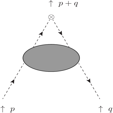
Figure 1: Momentum configuration for $\left\langle\psi(p){\cal O}^{i}(-p-q)\bar{\psi}(q)\right\rangle$.

Having defined the Green’s function the first step in its perturbative evaluation is the generation of the two loop Feynman graphs. To do this we have used the Qgraf package, [45], which produces $1$ one loop and $13$ two loop graphs. At the former order the expressions for the respective flavour non-singlet and singlet Green’s functions are the same irrespective of the subtraction point. The first place where any discrepancy will appear as a result of flavour symmetry in the chiral limit is at two loops and is due to the two graphs of Figure 2. This is because these graphs are zero for the flavour non-singlet case as the insertion of such an operator into the closed fermion loop gives a trace over a traceless flavour group generator. So such graphs will not contribute to $\Gamma^{{\cal I}^{ns}}$. By contrast for the flavour singlet case the graphs of Figure 2 will not be zero by this particular flavour trace argument. However for the operators ${\cal S}^{s}$, ${\cal T}^{s}$ and ${\cal P}^{s}$ the graphs of Figure 2 are zero since there are an odd number of $\gamma$-matrices in the closed loop in the chiral limit. These graphs would correspond to the disconnected graphs in the proton correlation function on the lattice. For ${\cal V}^{s}$ and ${\cal A}^{s}$ there will be an even number of $\gamma$-matrices in the loop in the massless case considered here. So these are the two possible instances of the flavour symmetry producing different two loop Green’s functions (2.3). As we will be using dimensional regularization in our calculations one concern that could be raised is whether this argument applies for operators containing $\gamma^{5}$. In the case of ${\cal A}^{ns}$ and ${\cal P}^{ns}$ we are permitted to use the naive anticommuting $\gamma^{5}$, [40, 41, 42], since it always appears in Feynman integrals in an open string of $\gamma$-matrices. It is its presence, or an odd number of them, within a closed fermion loop that requires special treatment in dimensional regularization, [40, 41, 42]. We will discuss this in detail later aside from noting that when $\gamma^{5}$, or an odd number of them, is present in a closed loop with an odd number of ordinary $\gamma$-matrices then the spinor trace is still zero as in four dimensions. Having taken flavour and Lorentz symmetries into account there is one final constraint to be considered however which is that corresponding to the colour vector space. All operators of (2.1) and (2.2) are colour singlets. In other words they do not include a colour group generator. So the colour trace is not the same as the parallel graphs contributing to the quark-gluon vertex function. In that instance if the operator insertion was replaced by a gluon then the sum of the fermion one loop subgraphs would be proportional to the structure constants $f^{abc}$. In the case of ${\cal V}^{s}$ the colour trace with one fewer group generator produces $\delta^{ab}$ which together with the relative minus sign arising from the respective $\gamma$-matrix traces means that the two graphs of Figure 2 sum to zero for this operator. For ${\cal A}^{s}$ by contrast while the colour argument applies equally, the presence of $\gamma^{5}$ in the spinor trace prevents the same procedure giving zero since the traces sum and are not equal and opposite. Therefore the only singlet operator that needs to be considered at any subtraction point, and not just the symmetric one, is ${\cal A}^{s}$ as it will produce contributions additional to its non-singlet partner.

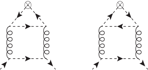
Figure 2: Extra graphs for flavour singlet operators.

Having isolated the only case we have to consider for singlet operators then in order to evaluate $\Gamma^{{\cal A}^{s}}$ we note that we have taken a different path to the partner computation of $\Gamma^{{\cal A}^{ns}}$ of [35, 36, 37]. To appreciate the contrast it is first best to summarize the earlier approach. In [35, 36, 37] a projection method was used whereby the Green’s function was decomposed into a basis of tensors consistent with the symmetries of the operator. For instance, for ${\cal V}$ this was

$${\cal P}^{\cal V}_{(1)\mu}(p,q) = \gamma_{\mu}~{}~{},~{}~{}{\cal P}^{\cal V}_{(2)\mu}(p,q)~{}=~{}\frac{p^{\mu}p\!\!\!/}{\mu^{2}}~{}~{},~{}~{}{\cal P}^{\cal V}_{(3)\mu}(p,q)~{}=~{}\frac{p_{\mu}q\!\!\!/}{\mu^{2}}~{},$$

$${\cal P}^{\cal V}_{(4)\mu}(p,q) = \frac{q_{\mu}p\!\!\!/}{\mu^{2}}~{}~{},~{}~{}{\cal P}^{\cal V}_{(5)\mu}(p,q)~{}=~{}\frac{q_{\mu}q\!\!\!/}{\mu^{2}}~{}~{},~{}~{}{\cal P}^{\cal V}_{(6)\mu}(p,q)~{}=~{}\Gamma_{(3)\,\mu pq}\frac{1}{\mu^{2}}$$ (2.5)

and this Lorentz basis for each bilinear operator Green’s function is the same whether the operator is flavour non-singlet or singlet. Here we have introduced the generalized $\gamma$-matrices of [42, 46, 47, 48, 49, 50] which are denoted by $\Gamma_{(n)}^{\mu_{1}\ldots\mu_{n}}$ and defined by

$$\Gamma_{(n)}^{\mu_{1}\ldots\mu_{n}}~{}=~{}\gamma^{[\mu_{1}}\ldots\gamma^{\mu_{n}]}$$ (2.6)

for integers $n$ with $0$ $\leq$ $n$ $<$ $\infty$. Each matrix is fully antisymmetric in the Lorentz indices for $n$ $\geq$ $2$ and the full set span the infinite dimensional spinor space when dimensional regularization is implemented. We note that $\Gamma_{(5)}^{\mu_{1}\mu_{2}\mu_{3}\mu_{4}\mu_{5}}$ is not related to $\gamma^{5}$ and in strictly four dimensions $\Gamma_{(n)}^{\mu_{1}\ldots\mu_{n}}$ $=$ $0$ for $n$ $\geq$ $5$. One advantage of these matrices is that they provide a natural partition since

$$\mbox{tr}\left(\Gamma_{(m)}^{\mu_{1}\ldots\mu_{m}}\Gamma_{(n)}^{\nu_{1}\ldots\nu_{n}}\right)~{}\propto~{}\delta_{mn}I^{\mu_{1}\ldots\mu_{m}\nu_{1}\ldots\nu_{n}}$$ (2.7)

with $I^{\mu_{1}\ldots\mu_{m}\nu_{1}\ldots\nu_{n}}$ denoting the unit matrix in $\Gamma$-space. Here we use the convention that when a momentum is contracted with a Lorentz index in $\Gamma_{(n)}^{\mu_{1}\ldots\mu_{n}}$ then the momentum itself appears in place of the index.

Once the basis for the Green’s function has been chosen then the coefficients of each tensor is deduced by multiplying it by a $d$-dimensional linear combination of the tensors to produce a sum of scalar Feynman integrals. These are then evaluated by applying the Laporta algorithm, [51], which systematically integrates by parts all the contributing graphs. This produces a linear combination of a small set of master integrals with $d$-dependent rational polynomial coefficients. For the symmetric point configuration explicit expressions for the one and two loop master integrals have been available for many years, [52, 53, 54, 55]. Though in more recent years they have been understood in the language of cyclotomic polynomials, [56]. To be explicit to two loops the Green’s functions with the kinematic configuration of (2.4) involve different linear combinations of numbers from the set

$$\left\{\mathbb{Q},\pi^{2},\zeta_{3},\zeta_{4},\psi^{\prime}(\mbox{\small{$\frac{1}{3}$}}),\psi^{\prime\prime\prime}(\mbox{\small{$\frac{1}{3}$}}),s_{2}(\mbox{\small{$\frac{\pi}{2}$}}),s_{2}(\mbox{\small{$\frac{\pi}{6}$}}),s_{3}(\mbox{\small{$\frac{\pi}{2}$}}),s_{3}(\mbox{\small{$\frac{\pi}{6}$}}),\frac{\ln^{2}(3)\pi}{\sqrt{3}},\frac{\ln(3)\pi}{\sqrt{3}},\frac{\pi^{3}}{\sqrt{3}}\right\}~{}.$$ (2.8)

Here $\zeta_{n}$ is the Riemann zeta-function, $s_{2}(z)$ and $s_{3}(z)$ are defined in terms of the polylogarithm function $\mbox{Li}_{n}(z)$

$$s_{n}(z)~{}=~{}\frac{1}{\sqrt{3}}\Im\left[\mbox{Li}_{n}\left(\frac{e^{iz}}{\sqrt{3}}\right)\right]$$ (2.9)

and $\psi(z)$ is the derivative of the logarithm of the Euler $\Gamma$-function. A final important aspect of the computation was the extensive use of symbolic manipulation which was facilitated through the use of the language Form and its threaded version Tform, [57, 58]. Using the Reduze package, [59, 60], written in C$++$ which implements the Laporta reduction we inserted the relations generated by the package for the required Feynman integrals via a Form module so that all our computations were carried out automatically. In addition we followed the prescription of [61] to implement the operator renormalization within the same automatic framework.

As we will be considering Green’s functions involving operators with $\gamma^{5}$ present we need to be careful in its treatment within dimensional regularization. Moreover the strategy we will choose to follow has to be robust in the sense that it should reproduce the known two loop symmetric point results of earlier work, [32, 33, 34, 35]. For the non-singlet example of ${\cal A}^{ns}$ and ${\cal P}^{ns}$ there are several ways one can proceed. First though we need to discuss the details of the Larin approach, [39], as general features of that computation will be used. It was inspired by and developed from the earlier one loop resolution of the treatment of $\gamma^{5}$ of [40, 41, 42, 62]. In reviewing [39] it is important to note that those calculations were carried out at an exceptional momentum configuration where the operator is inserted at zero momentum. In this case and also for the symmetric point, which is non-exceptional, for open strings of $\gamma$-matrices which include $\gamma^{5}$ matrices their naive anti-commutation with $d$-dimensional $\gamma$-matrices is valid. Related to this in [63] an extended set of (non-singlet) quark bilinear operators were considered in $d$-dimensions and renormalized in the dimensionally regularized theory. These were

$${\cal O}_{(n)}^{\mu_{1}\ldots\mu_{n}\,{ns}}~{}=~{}\bar{\psi}^{i}\Gamma_{(n)}^{\mu_{1}\ldots\mu_{n}}\psi^{j}$$ (2.10)

and in four dimensions they reduce to ${\cal S}^{ns}$, ${\cal V}^{ns}$ and ${\cal T}^{ns}$ respectively for $n$ $=$ $0$, $1$ and $2$. For $n$ $=$ $3$ and $4$ we have

$$\left.{\cal O}_{(3)}^{\mu\nu\sigma\,{ns}}\right|_{d=4}~{}=~{}\epsilon^{\mu\nu\sigma\rho}\bar{\psi}^{i}\gamma^{5}\gamma_{\rho}\psi^{j}~{}~{}~{},~{}~{}~{}\left.{\cal O}_{(4)}^{\mu\nu\sigma\rho\,{ns}}\right|_{d=4}~{}=~{}\epsilon^{\mu\nu\sigma\rho}\bar{\psi}^{i}\gamma^{5}\psi^{j}$$ (2.11)

where $\epsilon^{\mu\nu\sigma\rho}$ is the totally antisymmetric strictly four dimensional pseudo-tensor. Like $\gamma^{5}$ it has no existence outside strictly four dimensions. For $n$ $\geq$ $5$ the operators of (2.10) are evanescent in the sense that they are not present in strictly four dimensions due to their being more free Lorentz indices than the spacetime dimension which cannot be possible for a fully antisymmetric object.

Before concentrating on the technical details of the application of [39] to the operators we are interested in here, it is worth detailing the early treatment of $\gamma^{5}$. The problem of accommodating an object, such as $\gamma^{5}$ that only exists in strictly four dimensions, within dimensional regularization was recognised in the seminal work of [40]. In particular a formalism was developed in [40] that consistently took into account the analytic continuation of the spacetime dimension to a complex variable $d$ together with the algebraic properties of $\gamma^{5}$ that are only applicable in the underlying four dimensional physical subspace. The essence of the approach of [40] was to partition the $d$-dimensional spacetime into a physical four dimensional spacetime and a $(d-4)$-dimensional unphysical subspace. Purely four dimensional objects can only be elements of the former. Clear examples are $\gamma^{5}$ and $\epsilon^{\mu\nu\sigma\rho}$, which are present in (2.11), whose indices can only take values in the physical subspace. One test of this construction was the successful verification, [40], of the one loop axial vector anomaly of [64, 65, 66]. The full mathematical foundation for the treatment of $\gamma^{5}$ and $\epsilon^{\mu\nu\sigma\rho}$ in this partitioned spacetime was subsequently established in depth in [62]. While such a method can readily be applied at one loop level, effecting it in higher loop computations can only proceed in a reasonable amount of time and in practice through the use of automatic Feynman diagram computation. Enacting such an approach turns out to be difficult but an effective algorithm that equates to this procedure and, moreover can be encoded, was developed in [39] based on the ground work of [41, 42, 62]. In [67, 68] the definition of $\gamma^{5}$ in operators and currents adapted that introduced in [40, 41, 42, 62] and its relation to the renormalization procedure introduced in [41] was explored. In particular the additional finite renormalization that is necessary to ensure purely four dimensional symmetries are respected in the resulting finite theory after the regularization has been lifted, was determined to high loop order.

In light of this overview we now summarize its practical application to the multiplicatively renormalizable operators of interest, (2.10), at the symmetric point. Given the relation (2.11) between the generalized operators and their four dimensional counterparts, there is a connection with not only the renormalization of all the operators of (2.10) but importantly the respective Green’s functions themselves should be in full agreement in strictly four dimensions after renormalization, [41]. In other words the relation of (2.11) ought to be valid in the renormalized theory for any scheme. This algorithm of [41] was substantiated in [39] in the modified minimal subtraction ($\overline{\mbox{MS}}$) scheme through a two stage process. The first part was to renormalize the operators ${\cal O}_{(3)}^{\mu\nu\sigma\,{ns}}$ and ${\cal O}_{(4)}^{\mu\nu\sigma\rho\,{ns}}$, for example, separately in the usual way in the $\overline{\mbox{MS}}$ scheme to produce what is termed the naive renormalization constant for the $d$-dimensional operator. Aside from the one loop scheme independent term of the operator anomalous dimension the renormalization constants for the respective pairs ${\cal O}_{(0)}^{{ns}}$ and ${\cal O}_{(4)}^{\mu\nu\sigma\rho\,{ns}}$, and ${\cal O}_{(1)}^{\mu\,{ns}}$ and ${\cal O}_{(3)}^{\mu\nu\sigma\,{ns}}$ disagreed. We note that while $\Gamma_{(1)}^{\mu}$ and $\gamma^{\mu}$ are equivalent we will retain the former notation when we discuss the renormalization of the set of operators of the form (2.10). This disagreement in the naive renormalization constants is clearly not consistent with expectations from the naive anticommutation of $\gamma^{5}$ in four dimensions, [40, 41, 62]. However the second stage of the process developed in [41] is to recognise that it is not possible to retain the symmetry properties of a purely four dimensional entity, $\gamma^{5}$, in the dimensionally regularized theory. So to circumvent the absence of the four dimensional properties in the dimensionally regularized theory, one has to augment the naive renormalization of ${\cal O}_{(3)}^{\mu\nu\sigma\,{ns}}$ and ${\cal O}_{(4)}^{\mu\nu\sigma\rho\,{ns}}$ by including a finite renormalization constant pertinent to each operator, [41]. The condition used to define this in [39, 62] for the flavour non-singlet case was to impose the constraint that after the naive renormalization of the Green’s function with the $n$-index operator insertion the result is equivalent to that when $n$ is replaced by $(4-n)$, [39, 62]. Here $4$ is chosen as it is the critical dimension of QCD. There is a practical caveat to this in that the Lorentz tensor basis has to be written in terms of purely four dimensional objects first before the finite renormalization can be made. Also the finite renormalization constant in the $\overline{\mbox{MS}}$ scheme derives from the basis tensor corresponding to the tree term of the Green’s function.

For the fully symmetric point case we consider here we have adapted this approach but first checked that the previous non-singlet results are reproduced for $n$ $=$ $3$ and $4$. However for the Green’s functions of both operators the basis of tensors is larger than at the exceptional point. As a first step for $n$ $=$ $3$ and $4$ we have taken a slightly different tack to [35, 36, 37] and avoided using a projection method on the Green’s function. Instead to evaluate the contributing Feynman graphs we first removed all the $\gamma$-algebra from the Feynman integrals and evaluated the underlying tensor integrals. One reason for this is that it bypasses the complication of constructing a decomposition into a Lorentz basis with $3$ and $4$ free indices in the case of ${\cal A}^{ns}$ and ${\cal P}^{ns}$ respectively. In the latter case for instance that basis would include $\Gamma_{(6)}^{\mu\nu\sigma\rho pq}$ as one example. While this is evanescent it would have to be included to ensure the tensor basis was complete. So in avoiding a direct projection and consequently reproducing the same results as previous computations, [32, 33, 34, 35], will ensure that we have established a valid algorithm for handling $\gamma^{5}$ in the non-singlet case. This therefore will eventually be our strategy for the vector and axial vector operators in the singlet case when the complications due to the graphs of Figure 2 have to be taken into account. While the correct tensor basis will emerge from this integral projection the four dimensional basis of (2.5) will not be the relevant one for the naive renormalization of ${\cal A}^{ns}$. Using relations such as

$$\Gamma_{(3)}^{\mu\nu\sigma}~{}=~{}\epsilon^{\mu\nu\sigma\rho}\gamma^{5}\gamma_{\rho}~{}~{}~{},~{}~{}~{}\epsilon^{\mu\nu pq}\Gamma_{(1)\nu}~{}=~{}\gamma^{5}\Gamma_{(3)}^{\mu pq}$$ (2.12)

in four dimensions, for instance, the analogous basis will then be

$${\cal P}^{\cal A}_{(1)\mu}(p,q) = \gamma^{5}\gamma_{\mu}~{}~{},~{}~{}{\cal P}^{\cal A}_{(2)\mu}(p,q)~{}=~{}\gamma^{5}p\!\!\!/p^{\mu}\frac{1}{\mu^{2}}~{}~{},~{}~{}{\cal P}^{\cal A}_{(3)\mu}(p,q)~{}=~{}\gamma^{5}q\!\!\!/p_{\mu}\frac{1}{\mu^{2}}~{},$$

$${\cal P}^{\cal A}_{(4)\mu}(p,q) = \gamma^{5}p\!\!\!/q_{\mu}\frac{1}{\mu^{2}}~{}~{},~{}~{}{\cal P}^{\cal A}_{(5)\mu}(p,q)~{}=~{}\gamma^{5}q\!\!\!/q_{\mu}\frac{1}{\mu^{2}}~{}~{},~{}~{}{\cal P}^{\cal A}_{(6)\mu}(p,q)~{}=~{}\gamma^{5}\Gamma_{(3)\,pq\mu}\frac{1}{\mu^{2}}~{}.~{}~{}~{}~{}$$ (2.13)

Next we recall that to properly renormalize the operator ${\cal V}^{ns}$ requires some care. As the non-singlet vector current is conserved in the chiral limit

$$\partial_{\mu}\left(\bar{\psi}^{i}\gamma^{\mu}\psi^{j}\right)~{}=~{}0$$ (2.14)

its renormalization constant is unity to all orders in perturbation theory and in all renormalization schemes. In the $\overline{\mbox{MS}}$ scheme context this means that the Green’s function for ${\cal V}^{ns}$ is completely finite. However in a kinematic renormalization scheme where renormalization constants can have non-zero finite parts the renormalization constant for ${\cal V}^{ns}$ could mistakenly be chosen by demanding that the coefficient of ${\cal P}^{\cal V}_{(1)\mu}(p,q)$ is unity for instance. This would clearly contradict the general result that physical operators do not get renormalized. In practical terms the conservation of the currents is encoded in the quantum theory by a Ward-Takahashi identity. In the case of ${\cal V}^{ns}$ this corresponds to Green’s function of $\partial_{\mu}\left(\bar{\psi}^{i}\gamma^{\mu}\psi^{j}\right)$ being related to the quark $2$-point function. Therefore we have checked that for our integral projection construction that this is indeed the case in the $\overline{\mbox{MS}}$ scheme for the fully symmetric and hence non-exceptional configuration. We note that we found full agreement with the one and two loop results of [32, 33, 34, 35]. This was also checked in [63] for the direct projection on the operator Green’s function.

Since the non-singlet axial vector current is also conserved

$$\partial_{\mu}\left(\bar{\psi}^{i}\gamma^{5}\gamma^{\mu}\psi^{j}\right)~{}=~{}0$$ (2.15)

similar general reasoning also applies. Calculating the Green’s function of $\partial_{\mu}\left(\bar{\psi}^{i}\gamma^{5}\gamma^{\mu}\psi^{j}\right)$, however, it does not agree with $\gamma^{5}$ times the quark $2$-point function. This is consistent with Larin’s observation that treating the naive renormalization of the generalized operator ${\cal O}_{(3)}^{\mu\nu\sigma\,ns}$ as being equivalent to ${\cal A}^{ns}$ is incorrect. Instead an additional finite renormalization constant is required to ensure the consistency with symmetry properties of the strictly four dimensional theory. Ensuring the consistency with the quark $2$-point function in this case we find that to two loops at the symmetric point the finite renormalization is

$$Z^{\mbox{\footnotesize{fin}}}_{{\cal A}^{ns}}~{}=~{}1~{}-~{}4C_{F}a~{}+~{}\left[22C_{F}^{2}-\frac{107}{9}C_{F}C_{A}+\frac{4}{9}C_{F}T_{F}N_{\!f}\right]a^{2}~{}+~{}O(a^{3})$$ (2.16)

in full agreement with [39] where $a$ $=$ $g^{2}/(16\pi^{2})$ and $g$ is the gauge coupling constant. It should be stressed that we have verified that the finite renormalization is independent of the subtraction point which is a non-trivial observation.

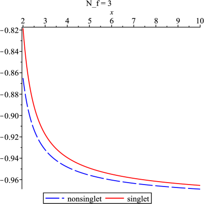
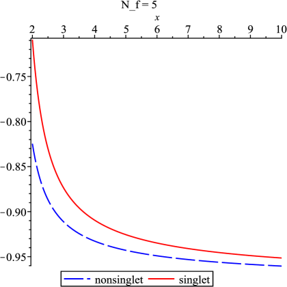
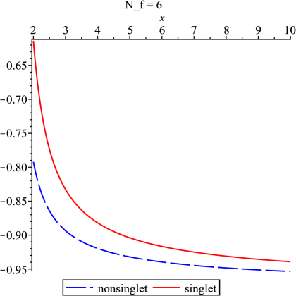
Figure 3: Comparison of two loop coefficient of $\gamma^{5}\gamma^{\mu}$ in $\Gamma^{{\cal A}^{ns}}$ and $\Gamma^{{\cal A}^{s}}$ for $N_{\!f}$ $=$ $3$ to $6$.

As can be seen in earlier work [32, 34, 35, 36, 37] the two loop explicit expression for (2.3) for each operator involves linear combinations of (2.8). These in principle could have been present in the two loop finite renormalization constant with our choice of (2.4). In the momentum configuration used in [39] only rational numbers or $\zeta_{3}$ were present in the finite parts of the Green’s function at three loops. So it is reassuring that the polylogarithms, for instance, of (2.8) are absent. We note that although the three loop finite renormalization is also known in the $\overline{\mbox{MS}}$ scheme, [39], in order to verify the next term of (2.16) at the symmetric point would require a new three loop computation. At present the three loop master integrals are not available in order to be able to perform this calculation. This comparison of the $n$ $=$ $1$ and $3$ Green’s function is in keeping with the spirit of [39, 62, 63]. However in the singlet case the presence of the extra graphs of Figure 2 will not make this a viable way to proceed as was indicated in [39]. In the non-singlet case the corresponding Ward-Takahashi identity for the axial vector operator provides a more field theoretic alternative method to determine the finite renormalization. In other words the Green’s function of $\partial_{\mu}\left(\bar{\psi}^{i}\gamma^{5}\gamma^{\mu}\psi^{j}\right)$ has to be equivalent to the quark $2$-point function multiplied by $\gamma^{5}$. To ensure this we have checked that the same gauge parameter independent finite renormalization constant, (2.16), is required. It should also be noted that we have checked that once this finite renormalization is determined from ensuring that the current conservation is preserved then the expressions for both Green’s functions of ${\cal V}^{ns}$ and ${\cal A}^{ns}$ are also in full agreement. By this we mean that the coefficients of ${\cal P}^{\cal I}_{(i)\mu}(p,q)$ for ${\cal O}^{ns}$ $=$ ${\cal V}^{ns}$ and ${\cal A}^{ns}$ are equal for each $i$ $=$ $1$ to $6$ and thus establishes the equivalence with Larin’s strategy in strictly four dimensions after renormalization.

One of the reasons for reviewing the non-singlet operator renormalization and indicating an alternative way of defining the finite renormalization constant is that it avoids the need to connect Green’s functions for different operators. For the singlet axial vector operator there is clearly no analogous partner. Instead as highlighted in [39, 62] the associated finite renormalization is derived from ensuring that the chiral anomaly is correctly restored in four dimensional Green’s function after renormalization. The non-singlet axial vector current is non-anomalous. Specifically the anomaly for the singlet case is given by

$$\partial_{\mu}\left(\bar{\psi}^{i}\gamma^{5}\gamma^{\mu}\psi^{i}\right)~{}=~{}aT_{F}N_{\!f}\epsilon^{\mu\nu\sigma\rho}G^{a}_{\mu\nu}G^{a}_{\sigma\rho}$$ (2.17)

where the right hand side can be written as a derivative of a gluonic current and (2.14) and (2.15) become partners in this alternative view of [39, 62]. In [39] the two loop finite renormalization constant was computed and is given by

$$Z^{\mbox{\footnotesize{fin}}}_{{\cal A}^{s}}~{}=~{}1~{}-~{}4C_{F}a~{}+~{}\left[22C_{F}^{2}-\frac{107}{9}C_{F}C_{A}+\frac{31}{9}C_{F}T_{F}N_{\!f}\right]a^{2}~{}+~{}O(a^{3})$$ (2.18)

which differs from (2.16) in the final two loop term. We have not reproduced this expression beyond one loop here due to a subtlety in (2.17). This is to do with the fact that both operators of (2.17) have first to be renormalized and the triangular mixing matrix of the operators determined, [39, 62]. Then to find $Z^{\mbox{\footnotesize{fin}}}_{{\cal A}^{s}}$ the anomaly equation itself, (2.17), has to be inserted in a Green’s function and evaluated in strictly four dimensions. In [39] this was carried out by inserting in a gluon $2$-point function where the momentum flowing into one of the external gluon legs vanishes. With a total derivative present due to having to take the divergence of the current, the momentum flow into the operator cannot be nullified. This momentum configuration allows one to use the Mincer algorithm, [69], which evaluates three loop massless $2$-point functions in dimensional regularization. A three loop calculation is in fact required to determine (2.18) due to the presence of the coupling constant $a$ on the right hand side of (2.17). This means that the loop order of the anomaly Green’s function and its coupling constant expansion are mismatched by one. Since this will also be the case for the symmetric point setup, the absence of the three loop master integrals for such Green’s function evaluations means that that calculation cannot be carried out at present. This also means that for the same reasons one cannot compute the two loop corrections to the singlet axial vector current conversion or matching function calculated at one loop in [32]. This function allows one to translate results between two different renormalization schemes and in the case of [32] the respective schemes were $\overline{\mbox{MS}}$ and the symmetric momentum subtraction (SMOM) scheme. As the conversion function is computed from the singlet axial vector current renormalization constants in the two schemes then the finite renormalization constant for restoring four dimensional symmetries through the Larin method will also be needed for this. In turn this requires the finite parts of the three loop Green’s function in both schemes. The absence of the three loop symmetric masters means that this cannot be carried out here. Having demonstrated, however, that the non-singlet axial vector finite $\overline{\mbox{MS}}$ renormalization constant consistently emerges in the symmetric point configuration, instead we merely accept the result (2.18) and use it for our $\overline{\mbox{MS}}$ computations. In other words we include the extra graphs of Figure 2 where ${\cal O}^{{\cal A}^{s}}$ is inserted. The $\gamma$-algebra is removed and the Lorentz tensor integrals evaluated by projection and the naive axial vector operator renormalization constant determined which is

$$Z_{{\cal A}^{s}}~{}=~{}1~{}+~{}\left[\frac{22}{3}C_{F}^{2}+\frac{10}{3}C_{F}T_{F}N_{\!f}\right]\frac{a^{2}}{\epsilon}~{}+~{}O(a^{3})~{}.$$ (2.19)

This is in full agreement with the expression given in [39]. Reproducing this is a check on our different projection strategy since the $O(a^{2})$ term arises purely from the graphs of Figure 2. After this naive renormalization the tensors of the Green’s function are mapped to their four dimensional counterparts and then the finite renormalization constant (2.18) is included. This ensures that the properties of the chiral anomaly are properly taken into consideration in the expression we have computed for the Green’s function of interest.

3 Results.

Having discussed the computational strategy in detail we now present our results for the singlet axial vector Green’s function. In order to give an indication of the structure of the final expression in four dimensions after the implementation of the Larin method we note that in the Landau gauge for $N_{\!f}$ $=$ $3$ we have

$$\left.\Gamma^{{\cal A}^{s}}_{\mu}\right|_{\alpha=0}^{N_{\!f}=3} = \left[-~{}1+\left[\frac{8}{3}+\frac{16}{81}\pi^{2}-\frac{8}{27}\psi^{\prime}(\mbox{\small{$\frac{1}{3}$}})\right]a\right.$$ (3.1)

$$~{}+\left.\left[\frac{887}{9}-\frac{12520}{27}s_{3}(\mbox{\small{$\frac{\pi}{6}$}})+\frac{10016}{27}s_{3}(\mbox{\small{$\frac{\pi}{2}$}})+\frac{2504}{9}s_{2}(\mbox{\small{$\frac{\pi}{6}$}})-\frac{5008}{9}s_{2}(\mbox{\small{$\frac{\pi}{2}$}})-\frac{1528}{27}\zeta_{3}\right.\right.$$

$$\left.\left.~{}~{}~{}~{}~{}~{}-\frac{3040}{243}\pi^{2}-\frac{760}{729}\pi^{4}+\frac{1520}{81}\psi^{\prime}(\mbox{\small{$\frac{1}{3}$}})+\frac{32}{243}\psi^{\prime}(\mbox{\small{$\frac{1}{3}$}})\pi^{2}-\frac{8}{81}\psi^{\prime}(\mbox{\small{$\frac{1}{3}$}})^{2}\right.\right.$$

$$\left.\left.~{}~{}~{}~{}~{}~{}+\frac{91}{243}\psi^{\prime\prime\prime}(\mbox{\small{$\frac{1}{3}$}})-\frac{9077}{4374\sqrt{3}}\pi^{3}-\frac{626}{27\sqrt{3}}\ln(3)\pi+\frac{313}{162\sqrt{3}}\ln^{2}(3)\pi\right]a^{2}\right]\gamma^{5}\gamma_{\mu}$$

$$+~{}\left[\left[\frac{32}{9}+\frac{32}{81}\pi^{2}-\frac{16}{27}\psi^{\prime}(\mbox{\small{$\frac{1}{3}$}})\right]a\right.$$

$$~{}~{}~{}~{}~{}+\left.\left[\frac{2428}{27}-\frac{6080}{9}s_{3}(\mbox{\small{$\frac{\pi}{6}$}})+\frac{4864}{9}s_{3}(\mbox{\small{$\frac{\pi}{2}$}})+\frac{1216}{3}s_{2}(\mbox{\small{$\frac{\pi}{6}$}})-\frac{2432}{3}s_{2}(\mbox{\small{$\frac{\pi}{2}$}})\right.\right.$$

$$\left.\left.~{}~{}~{}~{}~{}~{}~{}~{}~{}-\frac{808}{9}\zeta_{3}-\frac{5336}{243}\pi^{2}-\frac{3680}{2187}\pi^{4}+\frac{2668}{81}\psi^{\prime}(\mbox{\small{$\frac{1}{3}$}})+\frac{128}{729}\psi^{\prime}(\mbox{\small{$\frac{1}{3}$}})\pi^{2}\right.\right.$$

$$\left.\left.~{}~{}~{}~{}~{}~{}~{}~{}~{}-\frac{32}{243}\psi^{\prime}(\mbox{\small{$\frac{1}{3}$}})^{2}+\frac{148}{243}\psi^{\prime\prime\prime}(\mbox{\small{$\frac{1}{3}$}})-\frac{2204}{729\sqrt{3}}\pi^{3}-\frac{304}{9\sqrt{3}}\ln(3)\pi\right.\right.$$

$$\left.\left.~{}~{}~{}~{}~{}~{}~{}~{}~{}+\frac{76}{27\sqrt{3}}\ln^{2}(3)\pi\right]a^{2}\right]\left[\gamma^{5}p\!\!\!/p^{\mu}~{}+~{}\gamma^{5}q\!\!\!/q_{\mu}\right]\frac{1}{\mu^{2}}$$

$$+\left[\frac{16}{9}a\right.$$

$$~{}~{}~{}~{}+\left.\left[\frac{1214}{27}-\frac{6800}{27}s_{3}(\mbox{\small{$\frac{\pi}{6}$}})+\frac{5440}{27}s_{3}(\mbox{\small{$\frac{\pi}{2}$}})+\frac{1360}{9}s_{2}(\mbox{\small{$\frac{\pi}{6}$}})-\frac{2720}{9}s_{2}(\mbox{\small{$\frac{\pi}{2}$}})\right.\right.$$

$$\left.\left.~{}~{}~{}~{}~{}~{}~{}~{}-\frac{1280}{27}\zeta_{3}-\frac{1400}{81}\pi^{2}-\frac{880}{2187}\pi^{4}+\frac{700}{27}\psi^{\prime}(\mbox{\small{$\frac{1}{3}$}})+\frac{64}{729}\psi^{\prime}(\mbox{\small{$\frac{1}{3}$}})\pi^{2}\right.\right.$$

$$\left.\left.~{}~{}~{}~{}~{}~{}~{}~{}-\frac{16}{243}\psi^{\prime}(\mbox{\small{$\frac{1}{3}$}})^{2}+\frac{34}{243}\psi^{\prime\prime\prime}(\mbox{\small{$\frac{1}{3}$}})-\frac{2465}{2187\sqrt{3}}\pi^{3}-\frac{340}{27\sqrt{3}}\ln(3)\pi\right.\right.$$

$$\left.\left.~{}~{}~{}~{}~{}~{}~{}~{}+\frac{85}{81\sqrt{3}}\ln^{2}(3)\pi\right]a^{2}\right]\left[\gamma^{5}p\!\!\!/q_{\mu}~{}+~{}\gamma^{5}q\!\!\!/p_{\mu}\right]\frac{1}{\mu^{2}}$$

$$+\left[\left[\frac{32}{81}\pi^{2}-\frac{16}{27}\psi^{\prime}(\mbox{\small{$\frac{1}{3}$}})\right]a\right.$$

$$~{}~{}~{}~{}~{}+\left.\left[80s_{3}(\mbox{\small{$\frac{\pi}{6}$}})-64s_{3}(\mbox{\small{$\frac{\pi}{2}$}})-48s_{2}(\mbox{\small{$\frac{\pi}{6}$}})+96s_{2}(\mbox{\small{$\frac{\pi}{2}$}})-\frac{112}{9}\zeta_{3}+\frac{64}{27}\pi^{2}+\frac{224}{729}\pi^{4}\right.\right.$$

$$\left.\left.~{}~{}~{}~{}~{}~{}~{}~{}~{}-\frac{32}{9}\psi^{\prime}(\mbox{\small{$\frac{1}{3}$}})+\frac{64}{243}\psi^{\prime}(\mbox{\small{$\frac{1}{3}$}})\pi^{2}-\frac{16}{81}\psi^{\prime}(\mbox{\small{$\frac{1}{3}$}})^{2}-\frac{4}{27}\psi^{\prime\prime\prime}(\mbox{\small{$\frac{1}{3}$}})+\frac{29}{81\sqrt{3}}\pi^{3}\right.\right.$$

$$\left.\left.~{}~{}~{}~{}~{}~{}~{}~{}~{}+\frac{4}{\sqrt{3}}\ln(3)\pi-\frac{1}{3\sqrt{3}}\ln^{2}(3)\pi\right]a^{2}\right]\gamma^{5}\Gamma_{(3)\,pq\mu}\frac{1}{\mu^{2}}~{}+~{}O(a^{3})$$

for $SU(3)$ where the restriction also means that the symmetric point conditions of (2.4) have been implemented and $\alpha$ is the covariant gauge parameter. As a further check on the computation we note that the symmetry due to the interchange of the external legs of Figure 1 is present. This is the reason why pairs of basis tensors appear in the second and third terms and is consistent with the structure that emerged in the projection method used to evaluate $\Gamma^{{\cal A}^{ns}}$. The full expressions for the Green’s function for arbitrary $N_{\!f}$, linear covariant gauge parameter and general colour group are given in the attached data file. However to appreciate the relative size of the coefficients of each tensor for non-zero $N_{\!f}$ and $\alpha$ we note that the Landau gauge numerical value of $\left.\Gamma^{{\cal A}^{s}}_{\mu}\right|$ for $SU(3)$ is

$$\left.\Gamma^{{\cal A}^{s}}_{\mu}\right| = \left[~{}-~{}1+\left[-0.583194\alpha+1.624930\right]a\right.$$ (3.2)

$$\left.~{}+\left[-1.811999\alpha^{2}-3.222901\alpha+3.889852N_{\!f}+6.124832\right]a^{2}\right]\gamma^{5}\gamma_{\mu}$$

$$+\left[\left[0.305695\alpha+1.472082\right]a\right.$$

$$\left.~{}~{}+\left[1.095408\alpha^{2}+4.595782\alpha-7.001046N_{\!f}+18.797491\right]a^{2}\right]\left[\gamma^{5}p\!\!\!/p^{\mu}~{}+~{}\gamma^{5}q\!\!\!/q^{\mu}\right]\frac{1}{\mu^{2}}$$

$$+\left[\left[1.194584\alpha+1.777778\right]a\right.$$

$$\left.~{}~{}+\left[4.280593\alpha^{2}+12.109050\alpha-7.550907N_{\!f}+44.380585\right]a^{2}\right]\left[\gamma^{5}p\!\!\!/q^{\mu}~{}+~{}\gamma^{5}q\!\!\!/p^{\mu}\right]\frac{1}{\mu^{2}}$$

$$+\left[-~{}2.083473a\right.$$

$$\left.~{}~{}+\left[-0.173623\alpha^{2}-0.3484662\alpha+1.390610N_{\!f}-39.787370\right]a^{2}\right]\gamma^{5}\Gamma_{(3)\,pq\mu}\frac{1}{\mu^{2}}$$

$$+~{}O(a^{3})~{}.$$

Clearly the coefficient of the $\gamma^{5}\gamma^{\mu}$ term of the two loop Landau gauge Yang-Mills expression has the smallest magnitude in the $\overline{\mbox{MS}}$ scheme. In order to gauge the effect the inclusion of the graphs of Figure 2 have in comparison with the flavour non-singlet axial vector Green’s function it is instructive to compute the difference $(\Gamma^{{\cal A}^{ns}}_{\mu}$ $-$ $\Gamma^{{\cal A}^{s}}_{\mu})$. For example when $N_{\!f}$ $=$ $3$ then for $SU(3)$ we have

$$\left.\left[\Gamma^{{\cal A}^{ns}}_{\mu}~{}-~{}\Gamma^{{\cal A}^{s}}_{\mu}\right]\right|^{N_{\!f}=3} = \left[72-\frac{1120}{3}s_{3}(\mbox{\small{$\frac{\pi}{6}$}})+\frac{896}{3}s_{3}(\mbox{\small{$\frac{\pi}{2}$}})+224s_{2}(\mbox{\small{$\frac{\pi}{6}$}})-448s_{2}(\mbox{\small{$\frac{\pi}{2}$}})-\frac{112}{3}\zeta_{3}\right.$$ (3.3)

$$\left.~{}-\frac{416}{27}\pi^{2}-\frac{32}{81}\pi^{4}+\frac{208}{9}\psi^{\prime}(\mbox{\small{$\frac{1}{3}$}})+\frac{4}{27}\psi^{\prime\prime\prime}(\mbox{\small{$\frac{1}{3}$}})-\frac{406}{243\sqrt{3}}\pi^{3}\right.$$

$$\left.~{}-\frac{56}{3\sqrt{3}}\ln(3)\pi+\frac{14}{9\sqrt{3}}\ln^{2}(3)\pi\right]a^{2}\gamma^{5}\gamma_{\mu}$$

$$+\left[\frac{32}{3}-\frac{1600}{3}s_{3}(\mbox{\small{$\frac{\pi}{6}$}})+\frac{1280}{3}s_{3}(\mbox{\small{$\frac{\pi}{2}$}})+320s_{2}(\mbox{\small{$\frac{\pi}{6}$}})-640s_{2}(\mbox{\small{$\frac{\pi}{2}$}})-\frac{160}{3}\zeta_{3}\right.$$

$$\left.~{}~{}~{}-\frac{800}{27}\pi^{2}-\frac{64}{81}\pi^{4}+\frac{400}{9}\psi^{\prime}(\mbox{\small{$\frac{1}{3}$}})+\frac{8}{27}\psi^{\prime\prime\prime}(\mbox{\small{$\frac{1}{3}$}})-\frac{580}{243\sqrt{3}}\pi^{3}\right.$$

$$\left.~{}~{}~{}-\frac{80}{3\sqrt{3}}\ln(3)\pi+\frac{20}{9\sqrt{3}}\ln^{2}(3)\pi\right]\left[\gamma^{5}p\!\!\!/p^{\mu}~{}+~{}\gamma^{5}q\!\!\!/q^{\mu}\right]\frac{a^{2}}{\mu^{2}}$$

$$+\left[\frac{16}{3}-\frac{640}{3}s_{3}(\mbox{\small{$\frac{\pi}{6}$}})+\frac{512}{3}s_{3}(\mbox{\small{$\frac{\pi}{2}$}})+128s_{2}(\mbox{\small{$\frac{\pi}{6}$}})-256s_{2}(\mbox{\small{$\frac{\pi}{2}$}})-\frac{64}{3}\zeta_{3}\right.$$

$$\left.~{}~{}~{}-\frac{416}{27}\pi^{2}+\frac{208}{9}\psi^{\prime}(\mbox{\small{$\frac{1}{3}$}})-\frac{232}{243\sqrt{3}}\pi^{3}-\frac{32}{3\sqrt{3}}\ln(3)\pi\right.$$

$$\left.~{}~{}~{}+\frac{8}{9\sqrt{3}}\ln^{2}(3)\pi\right]\left[\gamma^{5}p\!\!\!/q^{\mu}~{}+~{}\gamma^{5}q\!\!\!/p^{\mu}\right]\frac{a^{2}}{\mu^{2}}$$

$$+\left[\frac{320}{3}s_{3}(\mbox{\small{$\frac{\pi}{6}$}})-\frac{256}{3}s_{3}(\mbox{\small{$\frac{\pi}{2}$}})-64s_{2}(\mbox{\small{$\frac{\pi}{6}$}})+128s_{2}(\mbox{\small{$\frac{\pi}{2}$}})+\frac{32}{3}\zeta_{3}-\frac{64}{27}\pi^{2}\right.$$

$$\left.~{}~{}~{}+\frac{64}{81}\pi^{4}+\frac{32}{9}\psi^{\prime}(\mbox{\small{$\frac{1}{3}$}})-\frac{8}{27}\psi^{\prime\prime\prime}(\mbox{\small{$\frac{1}{3}$}})+\frac{116}{243\sqrt{3}}\pi^{3}+\frac{16}{3\sqrt{3}}\ln(3)\pi\right.$$

$$\left.~{}~{}~{}-\frac{4}{9\sqrt{3}}\ln^{2}(3)\pi\right]\gamma^{5}\Gamma_{(3)\,pq\mu}\frac{a^{2}}{\mu^{2}}\,+\,O(a^{3})$$

which is independent of $\alpha$ or

$$\left.\left[\Gamma^{{\cal A}^{ns}}_{\mu}~{}-~{}\Gamma^{{\cal A}^{s}}_{\mu}\right]\right|^{N_{\!f}=3} = \left[10.960779\mu^{2}\gamma^{5}\gamma_{\mu}-17.013282\left[\gamma^{5}p\!\!\!/p^{\mu}~{}+~{}\gamma^{5}q\!\!\!/q^{\mu}\right]\right.$$ (3.4)

$$\left.~{}-14.060128\left[\gamma^{5}p\!\!\!/q^{\mu}~{}+~{}\gamma^{5}q\!\!\!/p^{\mu}\right]-4.856554\gamma^{5}\Gamma_{(3)\,pq\mu}\right]\frac{a^{2}}{\mu^{2}}$$

$$+~{}O(a^{3})$$

numerically.

Given this in order to appreciate the effect of the finite renormalization associated with the chiral anomaly in a clear way, it is instructive to plot (3.3) as a function of a dimensionless momentum variable. To achieve this we recall that solving the two loop $\beta$-function as a function of the squared momentum $Q^{2}$ and the QCD $\Lambda$ parameter gives

$$a_{2}(Q,\Lambda)~{}=~{}\frac{1}{b_{0}L}\left[1-\frac{b_{1}\ln(L)}{b_{0}^{2}L}\right]$$ (3.5)

where the $\beta$-function coefficients are, [70, 71, 72, 73],

$$b_{0} = \frac{11}{3}C_{A}~{}-~{}\frac{4}{3}T_{F}N_{\!f}$$

$$b_{1} = \frac{34}{3}C_{A}^{2}~{}-~{}4T_{F}C_{F}N_{\!f}~{}-~{}\frac{20}{3}T_{F}N_{\!f}C_{A}$$ (3.6)

in the $\overline{\mbox{MS}}$ scheme and we use the shorthand

$$L~{}=~{}\ln\left(\frac{Q^{2}}{\Lambda^{2}}\right)$$ (3.7)

for the logarithm which is present. In Figure 3 we have plotted the two loop coefficient of $\gamma^{5}\gamma^{\mu}$ for $\Gamma^{{\cal A}^{ns}}$ and $\Gamma^{{\cal A}^{s}}$ for several values of $N_{\!f}$ where the dimensionless variable $x$ is defined by $x$ $=$ $Q^{2}/\Lambda^{2}$. At $x$ $=$ $3$ for example, the difference between the coefficients of this particular tensor range from around $2\%$ to $7\%$ at $x$ $=$ $3$ from $N_{\!f}$ $=$ $3$ to $6$ respectively. As an alternative to the explicit values Figure 4 shows the difference for the same values of $N_{\!f}$ against $x$. Clearly at very high energy the discrepancy tends to zero.

Figure 4: Two loop coefficient of $\gamma^{5}\gamma^{\mu}$ in $\left[\Gamma^{{\cal A}^{ns}}\right.$ $-$ $\left.\Gamma^{{\cal A}^{s}}\right]$ for $N_{\!f}$ $=$ $3$ to $6$.

4 Discussion.

We have evaluated the two loop quark $2$-point function with the flavour singlet axial vector current inserted at non-zero momentum at the non-exceptional symmetric point. The main feature of this result is that unlike the one loop Green’s function we have had to ensure that our construction is consistent with the non-conservation of the singlet axial current due to the chiral anomaly. This was a non-trivial task since the use of dimensional regularization means that the purely four dimensional $\gamma^{5}$-matrix has to reconciled. To achieve this we implemented the Larin method, [39, 62], which was originally developed for the quark bilinear operators and founded upon [40, 41, 42, 62]. However, the finite renormalization constant associated with each $\gamma^{5}$ dependent operator was determined in [39, 62] for an exceptional momentum configuration. Here we have confirmed that these expressions for the flavour non-singlet operators are independent of the subtraction point for the renormalization scheme that we have used which is $\overline{\mbox{MS}}$. If one were to use another scheme such as the momentum subtraction scheme of [43, 44] then a different finite renormalization constant would emerge. For the flavour singlet axial vector case one would have to extend our two loop computation to three loops at the symmetric point to verify Larin’s two loop finite renormalization constant for that operator. This is due to the non-conserving part of the anomaly equation being proportional to the coupling constant.

Concerning the comparison of the axial vector flavour non-singlet and singlet corrections at two loops, the difference at a representative momentum scale is of the order of a few percent depending on the value of $N_{\!f}$. It is not clear whether such a value would make a significant difference to the analysis already carried out in [27, 32] for instance. It would depend on whether there is a clear signal in the lattice measurements to differentiate between the various Green’s functions. Of course this situation could be improved by extending to three loops which is the next natural step in the process. Aside from the absence of the three loop master integrals at the symmetric point, one would still have to be careful with the treatment of $\gamma^{5}$ in dimensional regularization. For instance, the finite renormalization constant for the axial vector current is known to three loops for the non-singlet case but only two loops for the singlet case. To put the latter on the same level as the former would require a four loop evaluation. While the computational tools are available through the development of the Forcer package, [74, 75], the treatment of $\gamma^{5}$ at four loops possibly requires detailed care. Recently there has been progress in this direction through the careful determination of the four loop Standard Model $\beta$-functions, [76]. This was achieved by ensuring general quantum field theory consistency conditions were satisfied for the $\gamma^{5}$ sector. By contrast for any treatment of $\gamma^{5}$ that uses the Larin approach where spinor traces involve a large number of $\gamma$-matrices it has been noted in [77] that one has always to be fully aware of potential hidden evanescence issues. In our case since we use (2.6) in dimensional regularization the latter point would need to be accommodated at three and higher loops.

Acknowledgements. This work was supported by a DFG Mercator Fellowship. The author thanks both Dr J. Green and Dr P.E.L. Rakow for discussions and comments on a draft, and to the former for indicating the necessity of this calculation. The Mathematical Physics Group at Humboldt University, Berlin is thanked for its hospitality where this work was initiated and partly carried out. Figures $1$ and $2$ were prepared with the Axodraw package, [78].

- [1] J. Ashman et al. European Muon Collaboration, Phys. Lett. B206 (1988), 364.
- [2] J. Ashman et al. European Muon Collaboration, Nucl. Phys. B328 (1989), 1.
- [3] C.A. Aidala, S.D. Bass, D. Hasch & G.K. Mallot, Rev. Mod. Phys. 85 (2013), 655.
- [4] P. Djawotho STAR Collaboration, Nuovo Cim. C036 (2013), 35.
- [5] A. Adare et al. PHENIX Collaboration, Phys. Rev. D90 (2014), 012007.
- [6] Y.-B. Yang, J. Liang, Y.-J. Bi, Y. Chen, T. Draper, K.-F. Liu & Z. Liu, Phys. Rev. Lett. 121 (2018), 212001.
- [7] V.D. Burkert, L. Elouadrhiri & F.X. Girod, Nature 557 (2018), 396.
- [8] P.E. Shanahan & W. Detmold, Phys. Rev. D99 (2019), 014511.
- [9] P.E. Shanahan & W. Detmold, Phys. Rev. Lett. 122 (2019), 072003.
- [10] M.J. Glatzmaier, K.-F. Liu & Y.-B. Yang, Phys. Rev. D95 (2017), 074513.
- [11] Y.-B. Yang, R.S. Sufian, A. Alexandru, T. Draper, M.J. Glatzmaier, K.-F. Liu & Y. Zhao, Phys. Rev. Lett. 118 (2017), 102001.
- [12] C. Alexandrou, M. Constantinou, K. Hadjiyiannakou, K. Jansen, C. Kallidonis, G. Koutsou, A.V. Avilés-Casco & C. Wiese, Phys. Rev. Lett. 119 (2017), 142002.
- [13] Y.-B. Yang, M. Gong, J. Liang, H.-W. Lin, K.-F. Liu, D. Pefkou & P. Shanahan, Phys. Rev. D98 (2018), 074506.
- [14] G.S. Bali, L. Barca, S. Collins, M. Gruber, M. Löffler, A. Schäfer, W. Söldner, P. Wein, S. Weishäupl & T. Wurm, JHEP 2005 (2020), 126.
- [15] G.S. Bali, S. Collins, M. Göckeler, R. Horsley, Y. Nakamura, A. Nobile, D. Pleiter, P.E.L. Rakow, A. Schäfer, G. Schierholz & J.M. Zanotti, Phys. Rev. Lett. 108 (2012), 222001.
- [16] M. Engelhardt, Phys. Rev. D86 (2012), 114510.
- [17] H.-W. Lin et al., Prog. Part. Nucl. Phys. 100 (2018), 107.
- [18] W. Detmold, R.G. Edwards, J.J. Dudek, M. Engelhardt, H.-W. Lin, S. Meinel, K. Originos & P. Shanahan, Eur. Phys. J. A55 (2019), 193.
- [19] X. Ji, Phys. Rev. Lett. 78 (1997), 610.
- [20] J. Liang, Y.-B. Yang, T. Draper, M. Gong & K.-F. Liu, Phys. Rev. D98 (2018), 074505.
- [21] H.-W. Lin, R. Gupta, B. Yoon, Y.-C. Jang & T. Bhattacharya, Phys. Rev. D98 (2018), 094512.
- [22] D. Djukanovic, H. Meyer, K. Ottnad, G. von Hippel, J. Wilhelm & H. Wittig, PoS LATTICE2019 (2019), 158.
- [23] A. Skouroupathis & H. Panagopoulos, Phys. Rev. D79 (2009), 094508.
- [24] A.J. Chambers, R. Horsley, Y. Nakamura, H. Perlt, P.E.L. Rakow, G. Schierholz, A. Schiller & J.M. Zanotti, Phys. Lett. B740 (2015), 30.
- [25] M. Constantinou, M. Hadjiantonis, H. Panagopoulos & G. Spanoudes, Phys. Rev. D94 (2016), 114513.
- [26] G.S. Bali, S. Collins, M. Göckeler, S. Piemonte & A. Sternbeck, PoS LATTICE2016 (2016), 187.
- [27] J. Green, N. Hasan, S. Meinel, M. Engelhardt, S. Krieg, J. Laeuchli, J. Negele, K. Orginos, A. Pochinsky & S. Syritsyn, Phys. Rev. D95 (2017), 114502.
- [28] D. Hatton, C.T.H. Davies, G.P. Lepage & A.T. Lytle, Phys. Rev. D100 (2019), 114513.
- [29] G. Martinelli, C. Pittori, C.T. Sachrajda, M. Testa & A. Vladikas, Nucl. Phys. B445 (1995), 81.
- [30] E. Franco & V. Lubicz, Nucl. Phys. B531 (1998), 641
- [31] N. Hasan, J. Green, S. Meinel, M. Engelhardt, S. Krieg, J. Negele, A. Pochinsky & S. Syritsyn, Phys. Rev. D99 (2019), 114505.
- [32] C. Sturm, Y. Aoki, N.H. Christ, T. Izubuchi, C.T.C. Sachrajda & A. Soni, Phys. Rev. D80 (2009), 014501.
- [33] M. Gorbahn & S. Jäger, Phys. Rev. D82 (2010), 114001.
- [34] L.G. Almeida & C. Sturm, Phys. Rev. D82 (2010), 054017.
- [35] J.A. Gracey, Eur. Phys. J. C71 (2011), 1567.
- [36] J.M. Bell & J.A. Gracey, Phys. Rev. D93 (2016), 065031.
- [37] J.A. Gracey, Phys. Rev. D99 (2019), 125017.
- [38] Y.-J. Bi, H. Cai, Y. Chen, M. Gong, K.-F. Liu, Z. Liu & Y.-B. Yang, Phys. Rev. D97 (2018), 094501.
- [39] S.A. Larin, Phys. Lett. B303 (1993), 113.
- [40] G. ’t Hooft & M. Veltman, Nucl. Phys. B44 (1972), 189.
- [41] T.L. Trueman, Phys. Lett. B88 (1979), 331.
- [42] D.A. Akyeampong & R. Delbourgo, Nuovo Cim. 17A (1973), 578.
- [43] W. Celmaster & R.J. Gonsalves, Phys. Rev. Lett. 42 (1979), 1435.
- [44] W. Celmaster & R.J. Gonsalves, Phys. Rev. D20 (1979), 1420.
- [45] P. Nogueira, J. Comput. Phys. 105 (1993), 279.
- [46] A.D. Kennedy, J. Math. Phys. 22 (1981), 1330.
- [47] A. Bondi, G. Curci, G. Paffuti & P. Rossi, Ann. Phys. 199 (1990), 268.
- [48] A.N. Vasil’ev, S.É. Derkachov & N.A. Kivel, Theor. Math. Phys. 103 (1995), 487.
- [49] A.N. Vasil’ev, M.I. Vyazovskii, S.É. Derkachov & N.A. Kivel, Theor. Math. Phys. 107 (1996), 441.
- [50] A.N. Vasil’ev, M.I. Vyazovskii, S.É. Derkachov & N.A. Kivel, Theor. Math. Phys. 107 (1996), 710.
- [51] S. Laporta, Int. J. Mod. Phys. A15 (2000), 5087.
- [52] A.I. Davydychev, J. Phys. A25 (1992), 5587.
- [53] N.I. Usyukina & A.I. Davydychev, Phys. Atom. Nucl. 56 (1993), 1553.
- [54] N.I. Usyukina & A.I. Davydychev, Phys. Lett. B332 (1994), 159.
- [55] T.G. Birthwright, E.W.N. Glover & P. Marquard, JHEP 0409 (2004), 042.
- [56] J. Ablinger, J. Blümlein & C. Schneider, J. Math. Phys. 52 (2011), 102301.
- [57] J.A.M. Vermaseren, math-ph/0010025.
- [58] M. Tentyukov & J.A.M. Vermaseren, Comput. Phys. Commun. 181 (2010), 1419.
- [59] C. Studerus, Comput. Phys. Commun. 181 (2010), 1293.
- [60] A. von Manteuffel & C. Studerus, arXiv:1201.4330 [hep-ph].
- [61] S.A. Larin & J.A.M. Vermaseren, Phys. Lett. B303 (1993), 334.
- [62] P. Breitenlohner & D. Maison, Comm. Math. Phys. 52 (1977), 11.
- [63] J.A. Gracey, Phys. Lett. B488 (2000), 175.
- [64] S.L. Adler, Phys. Rev. 177 (1969), 2426.
- [65] J.S. Bell and R. Jackiw, Nuovo Cim. A60 (1969), 47.
- [66] S.L. Adler and W. Bardeen, Phys. Rev. 182 (1969), 1517.
- [67] S.G. Gorishny & S.A. Larin, Phys. Lett. B172 (1986), 109.
- [68] S.A. Larin & J.A.M. Vermaseren, Phys. Lett. B259 (1991), 345.
- [69] S.G. Gorishny, S.A. Larin, L.R. Surguladze & F.K. Tkachov, Comput. Phys. Commun. 55 (1989), 381.
- [70] D.J. Gross & F.J. Wilczek, Phys. Rev. Lett. 30 (1973), 1343.
- [71] H.D. Politzer, Phys. Rev. Lett. 30 (1973), 1346.
- [72] W.E. Caswell, Phys. Rev. Lett. 33 (1974), 244.
- [73] D.R.T. Jones, Nucl. Phys. B75 (1974), 531.
- [74] T. Ueda, B. Ruijl & J.A.M. Vermaseren, PoS LL2016 (2016), 070.
- [75] T. Ueda, B. Ruijl & J.A.M. Vermaseren, Comput. Phys. Commun. 253 (2020), 107198.
- [76] J. Davies, F. Herren, C. Poole, M. Steinhauser & A.E. Thomsen, Phys. Rev. Lett. 124 (2020), 071803.
- [77] N. Zerf, Phys. Rev. D101 (2020), 036002.
- [78] J.C. Collins & J.A.M. Vermaseren, arXiv:1606.01177 [cs.OH].