Majorana-Kondo interplay in T-shaped double quantum dots

Abstract

The transport behavior of a double quantum dot side-attached to a topological superconducting wire hosting Majorana zero-energy modes is studied theoretically in the strong correlation regime. It is shown that Majorana modes can leak to the whole nanostructure, giving rise to a subtle interplay between the two-stage Kondo screening and the half-fermionic nature of Majorana quasiparticles. In particular, the coupling to the topological wire is found to reduce the effective exchange interaction between the two quantum dots in the absence of normal leads. Interestingly, it also results in an enhancement of the second-stage Kondo temperature when the normal leads are attached. Moreover, it is shown that the second stage of the Kondo effect can become significantly modified in one of the spin channels due to the interference with the Majorana zero-energy mode, yielding the low-temperature conductance equal to $G=G_{0}/4$, where $G_{0}=2e^{2}/h$, instead of $G=0$ in the absence of the topological superconducting wire. We also identify a nontrivial spin-charge ${\rm SU}(2)$ symmetry present in the system at a particular point in parameter space, despite lack of the spin nor charge conservation. Finally, we discuss the consequences of a finite overlap between two Majorana modes, as relevant for short Majorana wires.

I Introduction

Topological states of matter are in the center of current research in condensed matter physics Hasan and Kane (2010); Qi and Zhang (2011); Wang and Zhang (2017). This is due to the fact that such states are robust against decoherence and are thus very promising for applications in quantum information and computation Nayak et al. (2008). In this regard, topologically-protected states that form at the ends of one-dimensional topological superconductor, referred to as Majorana zero-energy modes Majorana (1937), provide an exciting example Kitaev (2003); Alicea (2012). The signatures of such Majorana quasiparticles have been recently reported in a number of experiments Mourik et al. (2012); Deng et al. (2012); Das et al. (2012); Albrecht et al. (2016); Deng et al. (2016, 2018); Zhang et al. (2018); Lutchyn et al. (2018); Gül et al. (2018).

It has been demonstrated that the detection of Majorana modes can be performed by measuring the current flowing through an adjacent quantum dot Deng et al. (2016). It turns out that the presence of Majorana zero-energy modes results in unique transport properties, including fractional values of the conductance $G$ Liu and Baranger (2011); Leijnse and Flensberg (2011); Cao et al. (2012); Gong et al. (2014); Liu et al. (2015); Weymann and Wójcik (2017); Liu et al. (2017); Prada et al. (2017); Ptok et al. (2017); Górski et al. (2018); Stenger et al. (2018); Cifuentes and Da Silva (2019); Silva et al. (2020). It has been shown that Majorana quasiparticles leaking into the neighboring dot weakly coupled to external contacts give rise to $G=(1/4)G_{0}$, where $G_{0}=2e^{2}/h$ Vernek et al. (2014); Ruiz-Tijerina et al. (2015). On the other hand, in the strong coupling regime, the Majorana-Kondo interplay determines the transport behavior of the system Golub et al. (2011); Lee et al. (2013); Cheng et al. (2014). At low temperatures, the quantum interference with a side-attached topological superconductor results in $G=(3/4)G_{0}$ Lee et al. (2013). Such fractional values of conductance reveal a half-fermionic nature of Majorana quasiparticles and may serve as signatures of the presence of these topologically-protected states in the system Aguado (2017); Lutchyn et al. (2018).

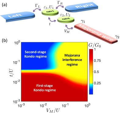
Figure 1: (a) Schematic of the considered system. The first quantum dot is coupled to the left and right metallic leads with coupling strengths $\Gamma_{L}$ and $\Gamma_{R}$, respectively. The second dot is coupled to the first one through the hopping $t$ and to the Majorana wire by $V_{M}$. The wire hosts Majorana quasiparticles described by operators $\gamma_{1}$ and $\gamma_{2}$. (b) The linear conductance as a function of $V_{M}$ and $t$ calculated at temperature $T=0.0005U$. For parameters see the main text and Fig. 3. Note that $G$ changes monotonically between different transport regimes.

In this paper we advance further the investigations of interplay between the Majorana zero-energy modes and correlations giving rise to the Kondo physics Kondo (1964); Hewson (1997); Goldhaber-Gordon et al. (1998), focusing on the system built of a double quantum dot side-coupled to a Majorana wire, as schematically shown in Fig. 1(a). The double dot is assumed to form with external contacts a T-shaped geometry, where only one of the dots is directly coupled to the leads, while the second dot is attached indirectly through the first quantum dot. This system, in the absence of Majorana wire, is known to exhibit a nonmonotonic dependence of conductance when lowering temperature due to the two-stage Kondo effect Pustilnik and Glazman (2001); Vojta et al. (2002); Cornaglia and Grempel (2005); Žitko and Bonča (2006); Chung et al. (2008); Sasaki et al. (2009). Moreover, the interplay between the Fano and Kondo effects in such systems was shown to give rise to interesting spin-resolved transport behavior Dias da Silva et al. (2013); Wójcik and Weymann (2014, 2015).

The main goal of this work is to uncover unique transport features resulting from the presence of Majorana quasiparticles and, in particular, to understand their influence on the two-stage Kondo effect. To achieve this goal in the most accurate way, we make use of the numerical renormalization group (NRG) method Wilson (1975); Bulla et al. (2008). We study the behavior of the spectral functions and the temperature dependence of the linear conductance, which reveal local extrema signaling the leakage of Majorana quasiparticles into the double dot system. Interestingly, we find that the quantum interference with Majorana zero-energy mode half-suppresses the spectral features related to the second-stage Kondo effect, giving rise to the fractional value of the linear conductance $G=(1/4)G_{0}$. This finding is presented in Fig. 1(b), which displays the conductance as a function of coupling to Majorana wire $V_{M}$ and the hopping between the dots $t$ plotted on logarithmic scale. One can clearly identify three different transport regimes. When the first-stage Kondo effect dominates $G=G_{0}$, on the other hand, when the system is in the second-stage Kondo regime $G$ becomes suppressed and reaches $G=0$. However, once the quantum interference with the Majorana wire becomes relevant the conductance is given by $G=(1/4)G_{0}$. This change from $G=0$ to $G=(1/4)G_{0}$ is a huge relative difference, giving better hope for an experimental observation as compared to the reduction of conductance from $G=G_{0}$ to $G=(3/4)G_{0}$, which is present in the case of a single quantum dot variant of the system.

Moreover, we show that due to the presence of Majorana quasiparticles the spectral function exhibits a unique five-peak structure, when the device is in the two-stage Kondo regime. We also demonstrate that, contrary to the expectations based on the analysis of excitation spectrum of double dot decoupled from normal contacts, increasing the coupling to topological superconductor actually enhances the second-stage Kondo temperature. A somewhat similar effect has been predicted for single quantum dots attached to Majorana wires, where an enhancement of the conventional Kondo temperature $T_{K}$ was observed Lee et al. (2013); Ruiz-Tijerina et al. (2015); Weymann and Wójcik (2017); Górski et al. (2018). In the T-shaped double quantum dot setup, at $T<T_{K}$, the spin of the second dot becomes screened by Fermi liquid formed by many-body Kondo state generated at the first quantum dot. Increasing the coupling to Majorana wire results then in an enhancement of the second-stage Kondo temperature $T^{*}$, similarly to the single quantum dot case where $T_{K}$ increases with $V_{M}$ Lee et al. (2013); Ruiz-Tijerina et al. (2015); Weymann and Wójcik (2017); Górski et al. (2018). At this point we would like to note that transport properties of a similar double dot system have been recently studied in the regime of relatively large inter-dot hopping Cifuentes and Da Silva (2019). However, the interplay of Majorana quasiparticles with the correlations giving rise to the two-stage Kondo screening has not been addressed so far, yet it manifest itself in spectral functions of all the parts of the nanostructure, as explained in Sec. IV.1.

The paper is structured as follows. The model, method and quantities of interested are presented in Sec. II. Then, Sec. III is devoted to the analysis of eigenspectrum of the effective Hamiltonian and the discussion of the effective exchange interaction between the dots. Sec. IV contains the main results of the paper and their discussion. Finally, the paper is summarized in Sec. V.

II Theoretical description

The considered system consists of a double quantum dot in a T-shaped geometry, i.e. with only one quantum dot attached directly to the leads and the second dot coupled to the first one through the corresponding hopping matrix elements. Additionally, the second quantum dot is coupled to a topological superconducting wire hosting Majorana zero-energy modes at its ends (Majorana wire). The schematic illustration of this system is presented in Fig. 1(a). The studied system can be described by the following Hamiltonian

$$H=H_{\rm Leads}+H_{\rm Tun}+H_{\rm DDM}.$$ (1)

Here, the first term models the left ($r=L$) and right ($r=R$) metallic leads as reservoirs of noninteracting quasiparticles

$$H_{\rm Leads}=\sum_{r=L,R}\sum_{\mathbf{k}\sigma}\varepsilon_{r\mathbf{k}}c^{\dagger}_{r\mathbf{k}\sigma}c_{r\mathbf{k}\sigma},$$ (2)

where $c_{r\mathbf{k}\sigma}^{\dagger}$ is the creation operator for an electron with spin $\sigma$, momentum $\mathbf{k}$ and energy $\varepsilon_{r\mathbf{k}}$ in the lead $r$. The second term of $H$ accounts for tunneling processes between the double quantum dot-Majorana wire subsystem and the normal leads. Because in the considered setup only the first dot is directly coupled to electrodes, the tunneling Hamiltonian simply reads

$$H_{\rm Tun}=\sum_{r=L,R}\sum_{\mathbf{k}\sigma}v_{r}\left(d^{\dagger}_{1\sigma}c_{r\mathbf{k}\sigma}+c^{\dagger}_{r\mathbf{k}\sigma}d_{1\sigma}\right),$$ (3)

with the corresponding tunnel matrix elements described by $v_{r}$ and assumed to be momentum independent. The operator $d^{\dagger}_{1\sigma}$ ($d_{1\sigma}$) is the creation (annihilation) operator of an electron with spin $\sigma$ in the first quantum dot. The coupling to external leads gives rise to the broadening of the first dot level, which can be described by $\Gamma_{r}=\pi\rho_{r}v_{r}^{2}$, where $\rho_{r}$ is the density of states of a given lead. In these considerations we assume a flat band of width $2D$ for each electrode and take $\Gamma_{L}=\Gamma_{R}\equiv\Gamma/2$. The band halfwidth is hereafter used as the energy unit $D\equiv 1$.

Finally, the last term of the Hamiltonian $H$ models the double dot-Majorana wire subsystem, and it can be written as

$$H_{\rm DDM} = \sum_{j=1,2}\sum_{\sigma}\varepsilon_{j}d_{j\sigma}^{\dagger}d_{j\sigma}+\sum_{j=1,2}U_{j}d_{j\uparrow}^{\dagger}d_{j\uparrow}d_{j\downarrow}^{\dagger}d_{j\downarrow}$$ (4)

$$+\sum_{\sigma}t(d_{1\sigma}^{\dagger}d_{2\sigma}+d_{2\sigma}^{\dagger}d_{1\sigma})$$

$$+\sqrt{2}V_{M}(d^{\dagger}_{2\downarrow}\gamma_{1}+\gamma_{1}d_{2\downarrow})+i\varepsilon_{M}\gamma_{1}\gamma_{2}.$$

Here, $d_{j\sigma}^{\dagger}$ is the creation operator for a spin-$\sigma$ electron on dot $j$ with the energy $\varepsilon_{j}$, and the two electrons residing on the same dot interact with the Coulomb correlation energy $U_{j}$. For the sake of clarity and convenience, we assume $U_{1}=U_{2}\equiv U$. The two quantum dots are coupled through the hopping matrix elements $t$. The coupling to the Majorana wire is described by the penultimate term of $H_{\rm DDM}$, where $V_{M}$ is the corresponding tunneling matrix element Flensberg (2010); Liu and Baranger (2011); Lee et al. (2013); Weymann and Wójcik (2017); Hoffman et al. (2017). The Majorana quasiparticles localized at the ends of the topological superconductor wire are described by the operators $\gamma_{1}$ and $\gamma_{2}$. The overlap between the wave functions of these two quasiparticles is described by $\varepsilon_{M}$. When the length of the Majorana wire is much larger than the superconducting coherence length, the two Majorana quasiparticles do not overlap and, consequently, $\varepsilon_{M}=0$ Albrecht et al. (2016). In the opposite case, $\varepsilon_{M}$ is finite, which results in a splitting of the energies of the Majorana quasiparticles. In the following we will refer to these two situations as the case of long/short Majorana wire.

The Majorana operators $\gamma_{1}$ and $\gamma_{2}$ can be represented by a fermionic operator $f$ as ${\gamma_{1}=(f^{\dagger}+f)/\sqrt{2}}$ and ${\gamma_{2}=i(f^{\dagger}-f)/\sqrt{2}}$, respectively. Then, the last two terms of $H_{\rm DDM}$ can be expressed as

$${\sqrt{2}V_{M}(d^{\dagger}_{2\downarrow}\gamma_{1}+\gamma_{1}d_{2\downarrow})} = {V_{M}(d^{\dagger}_{2\downarrow}-d_{2\downarrow})(f^{\dagger}+f)},$$ (5)

$$i\varepsilon_{M}\gamma_{1}\gamma_{2} = \varepsilon_{M}(f^{\dagger}f-1/2).$$ (6)

We note that since the Hamiltonian of the double dot coupled to normal leads possesses the full spin $SU(2)$ symmetry, one can choose the quantization axis in such a way that only one of the spin components couples to the Majorana mode Flensberg (2010); Liu and Baranger (2011); Lee et al. (2013). In our considerations, we assumed that the spin-down component is coupled to Majorana quasiparticles, cf. Eq. (4). However, to make the analysis more general, in Sec. IV.4 we also present the results for the case when the Majorana zero-energy modes are coupled to both spin projections Hoffman et al. (2017).

In this paper we are mainly interested in the linear response transport properties of the considered Majorana-double dot structure. The linear conductance between the left and right contacts can be then found from Meir and Wingreen (1992)

$$G=\frac{e^{2}}{h}\sum_{\sigma}\int\!d\omega\left[-f^{\prime}(\omega)\right]\pi\Gamma A_{\sigma}(\omega),$$ (7)

where $f^{\prime}(\omega)$ is the derivative of the Fermi-Dirac distribution function. $A_{\sigma}(\omega)$ denotes the spectral function of the first quantum dot for spin $\sigma$, $A_{\sigma}(\omega)=-\tfrac{1}{\pi}{\rm Im}G^{R}_{\sigma}(\omega)$, where $G^{R}_{\sigma}(\omega)\equiv\langle\!\langle d_{1\sigma}|d_{1\sigma}^{\dagger}\rangle\!\rangle_{\omega}^{R}$ is the Fourier transform of the retarded Green’s function $G^{R}_{\sigma}(t)=-i\Theta(t)\langle\{d_{1\sigma}(t),d_{1\sigma}^{\dagger}(0)\}\rangle$. To obtain the most reliable results and quantitatively understand the interplay of strong electron correlations with the presence of Majorana zero-energy modes, we use the numerical renormalization group method Wilson (1975); Bulla et al. (2008); NRG . In NRG calculations we use the discretization parameter $\Lambda=2$ and keep at least $3000$ states at each iteration. Moreover, to increase the accuracy of the spectral functions, which are typically subject to broadening issues Žitko and Pruschke (2009), we average the data over $4$ discretizations Campo and Oliveira (2005) and use the optimal broadening method Freyn and Florens (2009). On the other hand, the results presented for the linear conductance are obtained directly from the discrete NRG data, without the need of resorting to broadening Weymann and Barnaś (2013).

III Effective exchange interaction

In general, the low-temperature transport behavior of a system depends mostly on the low-energy part of the spectrum. In the T-shaped double quantum dot in the presence of normal leads the low-energy states relevant for the two-stage Kondo regime are those consisting of two singly-occupied quantum dots, organized into singlet and triplet, split by the effective antiferromagnetic exchange interaction $J_{\rm eff}\approx 4t^{2}/U$ Cornaglia and Grempel (2005). This structure remains untouched when the device is proximized by the conventional superconductor, only the value of $J_{\rm eff}$ increases (irrespective of the geometry), or even $J_{\rm eff}$ can arise due to the coupling to a BCS-like superconductor due to crossed Andreev reflection processes Wójcik and Weymann (2019). However, the situation qualitatively changes when the superconductor is topological.

To explore such a case, we define the basis states as $|\chi_{1}\chi_{2}n_{f}\rangle$, where $\chi_{1}$ and $\chi_{2}$ are the local states of quantum dots $1$ and $2$, with $\chi_{i}\in\{0,\uparrow,\downarrow,2\}$, and the Majorana zero-energy modes are described by the occupation of the auxiliary fermionic operator $f$, $n_{f}\in\{0,1\}$; cf. Eqs. (5) and (6). The local Hamiltonian consists then of $32$ states, nevertheless, the states relevant for the Kondo regime still consist of half-filled quantum dots. There are $8$ such states and we will refer to them as relevant states henceforth.

State				$Q_{P}$	$I$	$I_{z}$	Energy
$\alpha_{1}|{\rm s},\!1\rangle$ $\;+\;$	$\beta_{11}(|\!\downarrow\!20\rangle\!+\!|\!\uparrow\!00\rangle)/\sqrt{2}$ $\;+\;$	$\beta_{12}(|2\!\downarrow\!0\rangle\!+\!|0\!\uparrow\!0\rangle)/\sqrt{2}$ $\;+\;$	$\beta_{13}(|021\rangle\!+\!|201\rangle)/\sqrt{2}$	$-1$	$0$	$0$	$E^{0}_{++}$
$\alpha_{1}|{\rm s},\!0\rangle$ $\;+\;$	$\beta_{11}(|\!\downarrow\!21\rangle\!+\!|\!\uparrow\!01\rangle)/\sqrt{2}$ $\;+\;$	$\beta_{12}(|2\!\downarrow\!1\rangle\!+\!|0\!\uparrow\!1\rangle)/\sqrt{2}$ $\;+\;$	$\beta_{13}(|020\rangle\!+\!|200\rangle)/\sqrt{2}$	$+1$	$0$	$0$	$E^{0}_{++}$
$\alpha_{2}|\downarrow\downarrow 1\rangle$ $\;+\;$	$\beta_{21}|\!\downarrow\!00\rangle$ $\;+\;$	$\beta_{22}|0\!\downarrow\!0\rangle$ $\;+\;$	$\beta_{23}|001\rangle$	$-1$	$1$	$-1$	$E^{1}_{++}$
$\alpha_{3}|{\rm t},\!1\rangle$ $\;+\;$	$\beta_{31}(|\!\downarrow\!20\rangle\!-\!|\!\uparrow\!00\rangle)/\sqrt{2}$ $\;+\;$	$\beta_{32}(|0\!\uparrow\!0\rangle\!+\!|2\!\downarrow\!0\rangle)/\sqrt{2}$ $\;+\;$	$\beta_{33}(|201\rangle\!-\!|021\rangle)/\sqrt{2}$	$-1$	$1$	$0$	$E^{1}_{++}$
$\alpha_{4}|\uparrow\uparrow 1\rangle$ $\;+\;$	$\beta_{41}|\!\uparrow\!20\rangle$ $\;+\;$	$\beta_{42}|2\!\uparrow\!0\rangle$ $\;+\;$	$\beta_{43}|221\rangle$	$-1$	$1$	$+1$	$E^{1}_{++}$
$\alpha_{2}|\downarrow\downarrow 0\rangle$ $\;+\;$	$\beta_{21}|\!\downarrow\!01\rangle$ $\;+\;$	$\beta_{22}|0\!\downarrow\!1\rangle$ $\;+\;$	$\beta_{23}|000\rangle$	$-1$	$1$	$-1$	$E^{1}_{++}$
$\alpha_{3}|{\rm t},\!0\rangle$ $\;+\;$	$\beta_{31}(|\!\downarrow\!21\rangle\!-\!|\!\uparrow\!01\rangle)/\sqrt{2}$ $\;+\;$	$\beta_{32}(|0\!\uparrow\!1\rangle\!+\!|2\!\downarrow\!1\rangle)/\sqrt{2}$ $\;+\;$	$\beta_{33}(|200\rangle\!-\!|020\rangle)/\sqrt{2}$	$-1$	$1$	$0$	$E^{1}_{++}$
$\alpha_{4}|\uparrow\uparrow 0\rangle$ $\;+\;$	$\beta_{41}|\!\uparrow\!21\rangle$ $\;+\;$	$\beta_{42}|2\!\uparrow\!1\rangle$ $\;+\;$	$\beta_{43}|220\rangle$	$-1$	$1$	$+1$	$E^{1}_{++}$

Table 1: The eight lowest-energy eigenstates of the local Hamiltonian, Eq. (4), obtained for $\varepsilon_{1}=\varepsilon_{2}=-U/2$, $\varepsilon_{M}=0$ and $U_{1}=U_{2}=U$. For brevity the following notation for the singlet and triplet states, $|{\rm s},n_{f}\rangle=(|\downarrow\uparrow n_{f}\rangle-|\uparrow\downarrow n_{f}\rangle)/\sqrt{2}$ and $|{\rm t},n_{f}\rangle=(|\downarrow\uparrow n_{f}\rangle+|\uparrow\downarrow n_{f}\rangle)/\sqrt{2}$, was used. The first column presents the corresponding eigenstate, with $\alpha_{a}$ and $\beta_{ab}$ being the coefficients of the corresponding states. $I$ and $I_{z}$ stand for the isospin quantum numbers. Note that for $t,V_{M}\ll U$ the coefficient of the relevant state dominates, $|\alpha_{a}|\sim 1$. Moreover, after neglecting $\beta_{ab}$ the isospin $I$ becomes equivalent to the physical spin $\mathcal{S}$.

Furthermore, since in the considered model the Majorana mode couples to one spin channel, the spin $\mathcal{S}$ is no longer a good quantum number, nor are its components. Thus, the structure of the eigenbasis cannot be determined from the spin symmetry requirements. However, the system still exhibits two symmetries, namely, related to the conservation of fermion number parity, $Q_{P}=(-1)^{Q}$ [with $Q=f^{\dagger}f+\sum_{j\sigma}d^{\dagger}_{j\sigma}d_{j\sigma}$ denoting the fermion number] and the conservation of the number of spin-up electrons, $N_{\uparrow}=\sum_{j}d^{\dagger}_{j\uparrow}d_{j\uparrow}$ Bulla and Hewson (1997); Bradley et al. (1999). Moreover, for half-filled quantum dots (obtained in the model by setting $\varepsilon_{1}=\varepsilon_{2}=-U/2$) and long Majorana wire ($\varepsilon_{M}=0$), the Abelian symmetry related to the $N_{\uparrow}$ conservation is generalized to the full ${\rm SU}(2)$ isospin symmetry with its $z$ component defined as

$$I_{z}=\sum_{j}(d^{\dagger}_{j\uparrow}d_{j\uparrow}-\tfrac{1}{2}).$$ (8)

The operators rising and lowering $I_{z}$ can be defined as

$$I_{+}=\sum_{j}d^{\dagger}_{j\uparrow}\left[d_{j\downarrow}+(-1)^{j}d^{\dagger}_{j\downarrow}\right],$$ (9)

and $I_{-}=(I_{+})^{\dagger}$. Note that while the on-site ”spin-flip” part of $I_{+}$ (proportional to $d^{\dagger}_{j\uparrow}d_{j\downarrow}$) has always the same sign, the ”charge-flip” term has an alternating sign, analogously to the charge ${\rm SU}(2)$ symmetry generators. Importantly, the symmetry naturally extends to the full Wilson chain representation of the Hamiltonian (1) used in NRG calculations. This is done by allowing $j$ to run in the range $[-2,N]$ (with chain sites numbered from $0$ to $N$), where $j=-2$ and $j=-1$ correspond to the second and first quantum dot, which can be incorporated into the chain, and identifying $d_{-j\sigma}$ with the operator $f_{j\sigma}$ acting at the $j$-th site of the Wilson chain.

The isospin symmetry defined above can be easily recognized in the spectrum of the local Hamiltonian, $H_{\rm DDM}$. Its eigenenergies have the form

$$E^{I}_{\xi\zeta}=-\frac{U}{2}\left(1+\frac{\xi}{\sqrt{2}}\sqrt{A_{I}+\zeta\sqrt{B_{I}}}\right),$$ (10)

where indices $\xi,\zeta$ take values $\pm 1$ and

$$A_{1} = 1+4(t^{2}+2V_{M}^{2})U^{-2},$$

$$B_{1} = 1-8(t^{2}-2V_{M}^{2})U^{-2}+16t^{2}(t^{2}+4V_{M}^{2})U^{-4},$$

$$A_{0} = A_{1}+16t^{2}U^{-2},$$

$$B_{0} = B_{1}+32t^{2}U^{-2}+128t^{2}(t^{2}+4V_{M}^{2})U^{-4},$$

are constants of the order of unity. The four combinations of signs $(\xi,\zeta)$, together with four combinations of isospin and its $z$-component $(I,I_{z})$ corresponding to $I\leq 1$, and double degeneracy due to $Q_{P}$, give all the $32$ local states. The eigenenergies are plotted as a function of $V_{M}$, together with their degeneracy, are shown in Fig. 2.

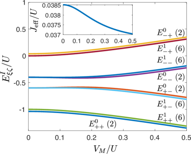
Figure 2: The eigenspectrum of the double dot-Majorana wire effective Hamiltonian, Eq. (4), calculated as a function of $V_{M}$ for $\varepsilon_{1}=\varepsilon_{2}=-U/2$, $t=0.1U$ and $\varepsilon_{M}=0$. The corresponding energies given by Eq. (10) are indicated, together with the degeneracy of states (numbers in brackets). The inset presents the effective exchange interaction $J_{\rm eff}\equiv E^{1}_{++}-E^{0}_{++}$.

For $U\gg t,V_{M}$, the order of magnitude of the energies given by Eq. (10) is determined by the signs of $\xi$ and $\zeta$. The lowest energies correspond to $\xi=+1$ and $\zeta=+1$, then $E^{I}_{++}\sim-U$; the other options lead to $E^{I}_{\xi\zeta}\sim-U/2$ or $E^{I}_{\xi\zeta}\sim 0$—up to the terms of the order of $U^{-2}$. For the analysis of the low-temperature properties only the former of these are important. Those states, together with their quantum numbers, are listed in Table 1. Note, that even though in general the eigenstates do not possess a definite spin $\mathcal{S}$, when projected onto the subspace spanned by the relevant states (when the coefficients $\beta_{ab}$, defined in Table 1, are neglected) they actually do, i.e. $I$ multiplets correspond to $\mathcal{S}$ multiplets with $I=\mathcal{S}$. In general, however, each of the $(I,I_{z})$ eigenstates is a superposition of a single relevant state with $(\mathcal{S},\mathcal{S}_{z})=(I,I_{z})$ and a number of other states, as presented in Table 1.

The relation between $\mathcal{S}$ and $I$ allows us actually to define the effective exchange interaction as the difference between the energies of the low-energy isospin singlet and triplet states,

$$J_{\rm eff} \equiv E^{1}_{++}-E^{0}_{++}$$ (11)

$$= \frac{U}{2\sqrt{2}}\left(\sqrt{A_{0}+\sqrt{B_{0}}}-\sqrt{A_{1}+\sqrt{B_{1}}}\right)$$

$$\approx \frac{4t^{2}}{U}\left[1-\left(\frac{2t}{U}\right)^{\!\!2}\!+2\left(\frac{2t}{U}\right)^{\!\!4}\!-5\left(\frac{2t}{U}\right)^{\!\!2}\!\left(\frac{2V_{M}}{U}\right)^{\!\!2}\right]$$

$$+\mathcal{O}(U^{-7}).$$

Note that the effect of coupling to topological superconductor becomes relevant only in the fifth order of expansion with respect to $1/U$. Clearly, from Eq. (11) one can conclude that the coupling to the Majorana wire slightly decreases the effective exchange interaction between the quantum dots. This can be explicitly seen in the inset to Fig. 2, which presents the dependence of $J_{\rm eff}=E^{1}_{++}-E^{0}_{++}$ on $V_{M}$. Despite very small magnitude of the decrease of $J_{\rm eff}$, one could expected a noticeable decrease of $T^{*}$, due to its exponential dependence on the inter-dot exchange; cf. Eq. (13). Interestingly, this effect is opposite to what happens in the presence of a conventional superconductor Wójcik and Weymann (2018, 2019). However, as shown in the following by accurate NRG calculations, the decrease of bare exchange interaction becomes overwhelmed by strong electron correlations. Actually, we demonstrate that increasing the coupling to topological wire results in an enhancement of the second-stage Kondo temperature $T^{*}$ instead of reduction, as one could expect from simple analysis of $H_{\rm DDM}$ spectrum, cf. Eq. (11).

We note that a similar effect has been predicted for single quantum dots coupled to normal leads and a topological superconductor, where increasing the coupling to Majorana wire gives rise to an enhancement of the Kondo temperature Lee et al. (2013); Ruiz-Tijerina et al. (2015); Weymann and Wójcik (2017); Górski et al. (2018). In the setup considered in this paper, at energy scales below the first-stage Kondo temperature $T_{K}$, the double dot system can be viewed as an effective single quantum dot attached to a conduction band of width $T_{K}$ (resulting from Fermi liquid formed by first quantum dot screened by lead conduction electrons) and additionally coupled to Majorana wire. Then, one could expect that increasing the coupling to topological wire would result in an increase of the relevant Kondo temperature (the second-stage Kondo temperature $T^{*}$), similarly as it does in the case of single quantum dots Lee et al. (2013); Ruiz-Tijerina et al. (2015); Weymann and Wójcik (2017); Górski et al. (2018). This picture wins over the local-Hamiltonian perspective presented in this section, as is shown by NRG calculations presented in the following.

IV Numerical results and discussion

We now turn to the numerical analysis of the transport behavior of the considered system. First, we consider the case of long Majorana wire and then also discuss the situation when there is a finite overlap between the Majorana quasiparticles. Finally, at the end, we examine the case when the Majorana wire is coupled to both spin projections of the double dot. To uncover the interplay between the Majorana and Kondo physics, we study the behavior of the relevant spin-resolved spectral functions as well as the temperature and gate voltage dependence of the linear conductance through the system.

To set the background for the following discussion, let us begin with a short introduction to the case of $V_{M}=0$. As already mentioned in the Introduction, in such a situation the system exhibits the two-stage Kondo effect, which is governed by two energy scales, $T_{K}$ and $T^{*}$ Cornaglia and Grempel (2005); Chung et al. (2008). With lowering the temperature, the Kondo effect develops on the first quantum dot once $T\lesssim T_{K}$, where the first-stage Kondo temperature $T_{K}$ for $\varepsilon_{1}=-U/2$ can be estimated from Haldane (1978)

$$T_{K}\approx\sqrt{\tfrac{\Gamma U}{2}}e^{-\pi U/8\Gamma}\,.$$ (12)

When the temperature is decreased further, such that $T\lesssim T^{*}$, the spin on the second quantum dot becomes screened by the Fermi liquid formed by first dot strongly coupled to the leads. The second-stage Kondo temperature $T^{*}$ can be evaluated from Cornaglia and Grempel (2005); Žitko and Bonča (2006); Wójcik and Weymann (2015)

$$T^{*}\approx\alpha T_{K}e^{-\beta T_{K}/J_{\rm eff}},$$ (13)

where $\alpha$ and $\beta$ are constants of the order of unity and $J_{\rm eff}\approx 4t^{2}/U$. This consecutive screening results in a nonmonotonic dependence of the spectral function on energy, see Fig. 3(a) for $V_{M}=0$, as well as a nonmonotonic temperature dependence of the linear conductance; for $G(T)$ in the case of $V_{M}=0$ see Figs. 8(a). When $T$ decreases, the conductance initially increases due to the first-stage Kondo effect, however, when the second spin experiences screening at even lower temperatures, it effectively scatters electrons transported through the central quantum dot and $G$ becomes suppressed.

As can be seen from Eqs. (12) and (13), both temperatures strongly depend on the relevant tunnel matrix elements and may be thus tuned by gate voltages. Moreover, because $T^{*}$ depends exponentially on the effective exchange interaction $J_{\rm eff}$ between the two quantum dots generated by the hopping $t$, changing $t$ results in large changes in $T^{*}$ [see also Fig. 8(a)]. We would also like to notice that recently the two-stage Kondo effect has been explored experimentally down to temperatures much lower than $T^{*}$ Guo et al. (2020).

IV.1 Spectral functions

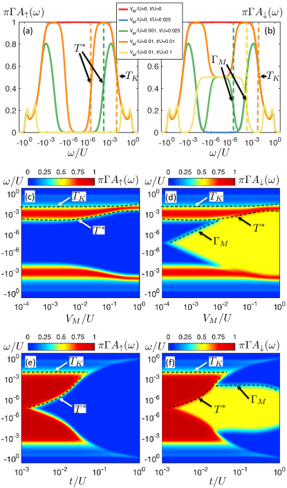
Figure 3: The normalized spectral function $\pi\Gamma A_{\sigma}(\omega)$ of the first quantum dot for (left column) spin-up and (right column) spin-down components. The first row presents the spectral function plotted as a function of energy $\omega$, where also the relevant energy scales are marked by vertical dashed lines. The next two rows display the density plots of the spectral function as function of energy and (c,d) the coupling to Majorana wire $V_{M}$ for $t/U=0.025$ and (e,f,) the hopping between the dots for $V_{M}/U=0.01$. The other parameters are: $U=0.2D$, $\varepsilon_{1}=\varepsilon_{2}=-U/2$, $\Gamma=0.1U$, where $D$ is the band halfwidth taken as energy unit $D\equiv 1$. Note the logarithmic scale on the axes.

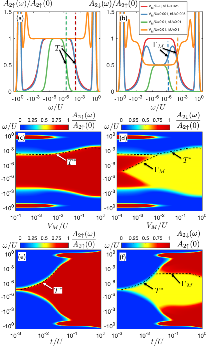
Figure 4: The same as in Fig. 3 calculated for the spectral function of the second quantum dot $A_{2\sigma}(\omega)$. The spectral function is normalized to its value at the Fermi energy for the spin-up component $A_{2\uparrow}(0)$. Note that in order to resolve the low-energy features in the density plots the color scale has been limited to $1$. However, the value of the spectral function at resonances $\omega=\pm-U/2$ can exceed $A_{2\uparrow}(0)$ depending on $t$, as can be seen in (a) and (b).

The spin-resolved spectral function of the quantum dot directly coupled to the normal leads is shown in Fig. 3. The first row shows $A_{\sigma}(\omega)$ for representative values of the coupling to Majorana wire $V_{M}$ and the hopping between the dots $t$. There are three different energy scales in the system that determine the transport behavior—these are marked with vertical dashed lines in Figs. 3(a) and (b). In the case of $t=V_{M}=0$, the system exhibits the usual spin-$1/2$ Kondo effect Hewson (1997). On the other hand, when the hopping between the dots is finite but $V_{M}=0$, one observes the conventional two-stage Kondo effect Cornaglia and Grempel (2005); Chung et al. (2008), see the blue line in the first row of Fig. 3. (Note, that this line coincides with the green line for $V_{M}/U=0.001$ and $t/U=0.025$ except for low energies in the spin-down component.) As can be seen in the figure, the spectral function first increases with lowering the energy $\omega$, which happens for $\omega\lesssim T_{K}$, but then starts to decrease once $\omega\lesssim T^{*}$.

The behavior of the spectral function changes when the coupling to Majorana wire is present. Note that in the effective Hamiltonian we assumed that the spin-down component of the dot’s spin couples to the Majorana quasiparticles. Thus, the largest effects related to the presence of topological superconductor can be expected in the behavior of $A_{\downarrow}(\omega)$. Nevertheless, finite $V_{M}$, through the Coulomb correlations, also affects the other spin component of the spectral function. As can be seen, the spin-up spectral function exhibits the usual two-stage Kondo dependence, with $A_{\uparrow}(\omega\to 0)\to 0$. This is just opposite to the case of the spin-down spectral function, where finite values of $V_{M}$ result in $A_{\downarrow}(0)=1/(2\pi\Gamma)$. Such a fractional value of the spectral function at the Fermi energy is a direct signature of a half-fermionic nature of Majorana quasiparticles. The coupling to Majorana wire half-suppresses the second-stage of the Kondo effect at a new energy scale $\Gamma_{M}$ resulting from the coupling to topological superconducting wire. As a consequence of this suppression, a five-peak structure can be visible in the spectral function of the first quantum dot, see the curves for $V_{M}/U=0.001$ and $t/U=0.025$, and for $V_{M}/U=0.01$ and $t/U=0.1$ in Fig. 3(b). $A_{\downarrow}(\omega)$ exhibits the usual Hubbard resonances for $\omega\approx\pm U/2$ (note that $\varepsilon_{1}=\varepsilon_{2}=-U/2$). Then, with lowering $\omega$, $A_{\downarrow}(\omega)$ starts growing due to the Kondo effect, however, it becomes suppressed once $\omega\approx T^{*}$ due to the second-stage Kondo screening, which results in a local maximum around $\omega\approx T_{K}$. With further decrease of $\omega$, the Majorana energy scale $\Gamma_{M}$ comes into play, destroying the second-stage Kondo effect and resulting in a further resonance just at the Fermi energy. This happens when the coupling to the Majorana wire is smaller than the hopping $t$. On the other hand, when the coupling to Majorana wire is comparable to the hopping, see the case for $V_{M}/U=t/U=0.01$ in Figs. 3(a) and (b), both spin resolved spectral functions exhibit a four-peak structure due to the two-stage Kondo effect. However, the spin-down component does not drop to zero at the Fermi energy such as its spin-up counterpart, but retains finite value of $A_{\downarrow}(0)=1/(2\pi\Gamma)$.

In turn, we analyze how the relevant energy scales change with both $V_{M}$ and $t$. The second row of Fig. 3 presents the density plots of the spectral function versus $V_{M}$ calculated for $t/U=0.025$. For the spin-up component, it is clearly evident that the coupling to Majorana wire strongly affects the second stage Kondo temperature $T^{*}$, i.e. $T^{*}$ grows with increasing $V_{M}$. It is also interesting to note that, although $T^{*}$ strongly depends on $V_{M}$, the behavior of $A_{\uparrow}(\omega\to 0)$ does not depend on the coupling to the Majorana wire and one has $A_{\uparrow}(\omega\to 0)\to 0$. In the case of $A_{\downarrow}(\omega)$, one observes that for relatively small values of the coupling to Majorana wire, the low-energy behavior of the spectral function starts changing. A plateau of $A_{\downarrow}(0)=1/(2\pi\Gamma)$ develops at low energies once the energy scale becomes smaller than $\Gamma_{M}$, see Fig. 3(d). With increasing $V_{M}$ further, $\Gamma_{M}$ merges with $T^{*}$ and the characteristic five-peak structure disappears. Then, an enhancement of $T^{*}$ with increasing $V_{M}$ can be observed.

The dependence of $A_{\sigma}(\omega)$ on $t$ for $V_{M}/U=0.01$ is presented in Figs. 3(e) and (f). Since $T^{*}$ depends strongly on $t$, the region of $A_{\uparrow}(\omega)\approx 1/\pi\Gamma$ for $T^{*}\lesssim T\lesssim T_{K}$ shrinks as $t$ grows and, e.g. for $t/U=\Gamma/U=0.1$, the spectral function displays only a small resonance, see Fig. 3(e). This is characteristic of the local singet regime, where the Kondo effect on the first quantum dot does not develop, but the two dots form a molecular singlet state. The two-stage Kondo regime can be reached from this phase by reducing the hopping $t$. We note that even though this is a continuous crossover, it is related to switching on or off many-body Kondo correlations. Namely, for large $t$ the Kondo effect is absent, while for small values of the hopping between the dots the many-body Kondo state develops. Interestingly, when $T^{*}$ becomes larger than the Majorana energy scale $\Gamma_{M}$, an additional resonance at the Fermi energy of halfwidth $\sim\Gamma_{M}$ forms in the spin-down spectral function.

To make the discussion more comprehensive, we now analyze the behavior of the spectral function of the second quantum dot $A_{2\sigma}(\omega)$, which is presented in Fig. 4. This figure is calculated for the same parameters as Fig. 3 and presents the same dependencies. The spectral function is normalized to the value of the spin-up component taken at the Fermi energy $A_{2\uparrow}(0)$. When the system is in the two-stage Kondo regime, the spin-up spectral function displays a plateau at low energies of halfwidth $\sim T^{*}$. On the other hand, the spin-down spectral function also exhibits a plateau of the same width, but half-reduced magnitude, i.e. $A_{2\downarrow}(0)=A_{2\uparrow}(0)/2$. This is the signature of the presence of Majorana zero-energy mode and its half-fermionic nature. The density plots of $A_{2\sigma}(\omega)$ presented in Fig. 4 clearly reveal the behavior of the relevant energy scales, which is similar to that shown in Fig. 3. One can conclude, that the signatures of the Majorana physics are visible in the spectra of both quantum dots, and it is not justified to prescribe the presence of a Majorana quasiparticle to any of them.

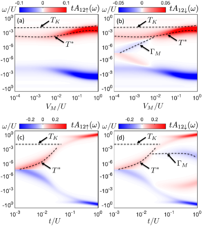
Figure 5: The spectral function $A_{12\sigma}(\omega)$ for (a,c) spin-up and (b,d) spin-down components plotted as function of energy and (a,b) the coupling to Majorana wire $V_{M}$ for $t/U=0.025$ and (c,d) the hopping between the dots $t$ for $V_{M}/U=0.01$. The other parameters are the same as in Fig. 3. Note the logarithmic scale on both axes.

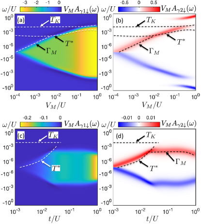
Figure 6: The spectral functions (a,c) $A_{\gamma 1\downarrow}(\omega)$ and (b,d) $A_{\gamma 2\downarrow}(\omega)$ plotted as function of energy and (a,b) the coupling to Majorana wire $V_{M}$ for $t/U=0.025$ and (c,d) the hopping between the dots $t$ for $V_{M}/U=0.01$. The other parameters are the same as in Fig. 3. Note the logarithmic scale on both axes.

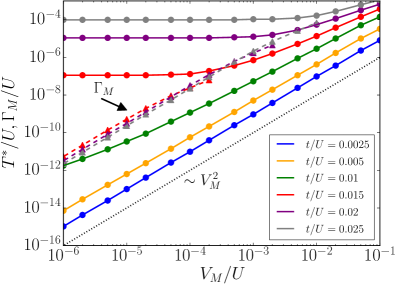
Figure 7: The second-stage Kondo temperature $T^{*}$ and the Majorana energy scale $\Gamma_{M}$ plotted as a function of $V_{M}$ for several values of the hopping between the quantum dots $t$. The other parameters are the same as in Fig. 3. The solid (dashed) line presents $T^{*}$ ($\Gamma_{M}$). Note the logarithmic scale in both axes.

Further insight into the leakage of Majorana states into the double dot setup can be obtained from the analysis of off-diagonal spectral functions, representing the correlations between the two quantum dots, $A_{12\sigma}(\omega)=-\tfrac{1}{\pi}{\rm Im}\langle\!\langle d_{1\sigma}|d_{2\sigma}^{\dagger}\rangle\!\rangle_{\omega}^{R}$, as well as between the Majorana quasiparticle and electrons in the first and second quantum dot, $A_{\gamma 1\downarrow}(\omega)=-\tfrac{1}{\pi}{\rm Im}\langle\!\langle\gamma|d_{1\downarrow}^{\dagger}\rangle\!\rangle_{\omega}^{R}$ and $A_{\gamma 2\downarrow}(\omega)=-\tfrac{1}{\pi}{\rm Im}\langle\!\langle\gamma|d_{2\downarrow}^{\dagger}\rangle\!\rangle_{\omega}^{R}$, respectively. These spectral functions are presented in Figs. 5 and 6 for the same parameters as used in Figs. 3-4. The spectral function $A_{12\sigma}(\omega)$ has been normalized by the hopping $t$, whereas $A_{\gamma j\downarrow}(\omega)$ is normalized by $V_{M}$. To facilitate the comparison, we have also included the corresponding dashed lines presenting the relevant energy scales.

Let us begin the discussion with $A_{12\sigma}(\omega)$, which describes the cross-correlations between the two quantum dots. The spin-up component exhibits two patterns at energies approximately corresponding to $\pm T^{*}$, which strongly depend on the value of hopping and depart from the Fermi energy as $t$ grows, see Fig. 5(c). Finite coupling to topological wire influences $A_{12\uparrow}(\omega)$ only for relatively large $V_{M}\gtrsim t$, and shifts the resonances in $|A_{12\uparrow}(\omega)|$ to higher energies, see Fig. 5(a). New features can be expected in the behavior of the opposite spin component, which is directly coupled to the Majorana mode. Indeed, in Fig. 5(b) one can see that, as $V_{M}$ increases, new resonances emerge at energy scale $\omega\approx\pm\Gamma_{M}$. Moreover, similar features are visible in Fig. 5(d), which presents $A_{12\downarrow}(\omega)$ calculated while changing the hopping between the dots $t$. It can be nicely seen that only if the hopping becomes relatively large, Majorana mode can leak into the quantum dots. We also note that the features related to the presence of Majorana modes result in the difference in the magnitude of spin components of $A_{12\sigma}(\omega)$, such that $A_{12\uparrow}(\omega)/A_{12\downarrow}(\omega)=2$.

To examine how exactly the Majorana state appears in the two dots, in Fig. 6 we show the correlation function between the Majorana quasiparticle and electrons in each of the quantum dots. First of all, one can see that the behavior of $A_{\gamma 1\downarrow}(\omega)$ is completely different compared to that of $A_{\gamma 2\downarrow}(\omega)$, although the features related to Majorana mode occur at approximately comparable energy scales in both spectral functions. While $A_{\gamma 1\downarrow}(\omega)$ displays a plateau for $|\omega|\lesssim\Gamma_{M}$, $A_{\gamma 2\downarrow}(\omega)$ exhibits a peak/dip for positive/negative energy when $\omega\approx\pm\Gamma_{M}$. The position of these features grows with $V_{M}$, see the first row of Fig. 6. The corresponding spectral functions plotted vs the hopping $t$ are shown in the second row of the figure. It is seen that the energy associated with Majorana features grows with $t$, however, once $t\gtrsim V_{M}$, the dependence saturates, see Figs. 6(c) and (d).

Let us now examine how the magnitude of the second-stage Kondo temperature $T^{*}$ and the characteristic Majorana energy scale $\Gamma_{M}$ depend on the coupling to topological wire. There quantities as a function of $V_{M}$ are shown in Fig. 7 and are plotted for selected values of the hopping between the dots $t$. $T^{*}$ was estimated as an energy scale at which the spin-up spectral function drops to half of its maximum value with decreasing the energy $\omega$. On the other hand, the Majorana energy scale $\Gamma_{M}$ was determined from the energy at which the spin-down spectral function drops from $1/(2\pi\Gamma)$ at $\omega\to 0$ to the half of its minimum value as the energy increases, cf. Figs. 3(a)-(b) and 4(a)-(b). Note that in this way we can extract $\Gamma_{M}$ only for certain range of parameters, i.e. when $\Gamma_{M}\lesssim T^{*}$.

It can be nicely seen that $T^{*}\propto V_{M}^{2}$ for low values of the hopping between the dots, i.e. when the increase of $T^{*}$ is just due to the coupling to Majorana wire, see e.g. the case of $t/U=0.0025$ in Fig. 7. However, when $t$ increases, a larger value of $V_{M}$ is needed in order to affect $T^{*}$. Nevertheless, once this happens, $\Gamma_{M}$ again scales quadratically with $V_{M}$. On the other hand, if $T^{*}$ is relatively large, increasing $V_{M}$ does not have any effect on the second-stage Kondo temperature, see the curves for $t/U\geq 0.015$ for low values of $V_{M}$. In other words, the influence of $V_{M}$ on the behavior of $A_{\uparrow}(\omega)$ is negligible. This is just contrary to $A_{\downarrow}(\omega)$, which exhibits then new features due to quantum interference with Majorana zero-energy mode, resulting in an additional resonance at the Fermi energy. As can be seen in Fig. 7 where $\Gamma_{M}$ is presented by dashed lines, $\Gamma_{M}\propto V_{M}^{2}$, similarly to $T^{*}$. Note also that the Majorana scale does not depend on the hopping between the dots—the curves presenting $\Gamma_{M}$ for different $t$ almost overlap, see Fig. 7.

As follows from the discussion presented in this section, the signatures of Majorana states are clearly visible in both quantum dots. Majorana correlations leak into the double dot giving rise to unique spectral features, which in case of $A_{\sigma}(\omega)$ and $A_{2\sigma}(\omega)$ could be in principle probed with an STM tip. Importantly, all the spin-down spectral functions reveal the energy scales related to the Majorana zero-energy mode, which allows to conclude that Majorana correlations are present in the whole nanostructure, not only at one of the quantum dots. Nevertheless, because in our setup it is the spectral function of the first dot, which is directly related to the conductance through the system, cf. Eq. (7), from now on let us restrict ourselves to the discussion of the behavior of $A_{\sigma}(\omega)$.

IV.2 Linear conductance

The interplay between the Majorana and Kondo physics gives rise to well-resolved features visible in the behavior of the linear conductance through the system. First, let us discuss the temperature dependence of $G$, whereas later on we turn to the analysis of the conductance dependence on the gate voltage.

IV.2.1 Temperature dependence

The spin-resolved linear conductance as a function of temperature calculated for different values of hopping between the dots and the coupling to the Majorana wire is presented in Figs. 8 and 9. While the first figure displays $G(T)$ calculated for selected values of $V_{M}$ while tuning $t$, the second figure presents a complementary picture: $G(T)$ determined for a few values of $t$ while changing $V_{M}$. These figures nicely demonstrate the evolution of the relevant energy scales in the system.

The spin-up component of the linear conductance exhibits a typical nonmonotonic dependence due to the two-stage Kondo effect Cornaglia and Grempel (2005). First, with lowering the temperature, the conductance increases due to the Kondo effect, however, around $T\approx T^{*}$, it starts to drop due to the second stage of screening, at which the spin of the second dot becomes screened. Since the second-stage Kondo temperature depends strongly on the coupling to the Majorana wire, increasing $V_{M}$ results in an enhancement of $T^{*}$. As a consequence, the maximum value of the conductance, which develops for $T^{*}\lesssim T\lesssim T_{K}$ becomes reduced, see the left columns of Figs. 8 and 9.

The enhancement of the second stage of Kondo screening with raising $V_{M}$ (due to the increase of $T^{*}$) is clearly visible in the left column of Fig. 9. This enhancement is more pronounced when the hopping between the dots is relatively small. As shown in Fig. 9(a), it is the coupling to Majorana wire that actually generates the second-stage of Kondo screening. This is because $T^{*}$ for $t/U=10^{-2}$ is smaller than the energy scale presented in the figure. However, when $t$ grows, larger values of coupling to Majorana wire are needed in order to give rise to an increase of $T^{*}$. Nevertheless, the advantageous impact of the coupling to the topological wire on $T^{*}$ is clearly visible.

On the other hand, the spin-down conductance reveals much richer behavior due to the Majorana-Kondo interplay. When the hopping between the dots is relatively small, see Fig. 9(e) for $t/U=0.01$, $T^{*}$ for $V_{M}=0$ is smaller than the energy range considered in the figure and a pronounced Kondo plateau is visible in the conductance. Turning on the coupling to the Majorana wire, results in a drop of conductance to $G_{\downarrow}=(1/4)G_{0}$ at the characteristic energy scale $\omega\approx\Gamma_{M}$, which grows with increasing $V_{M}$. When the hopping between the dots becomes increased, such that the second-stage Kondo screening can be visible in the behavior of the spin-up conductance, one can observe an interplay between the Kondo effect and Majorana-induced quantum interference. When $\Gamma_{M}\lesssim T^{*}$, a dip develops in the linear conductance and $G_{\downarrow}(T)$ exhibits two local maxima, see e.g. Figs. 8(f)-(g) and Figs. 9(f)-(g). On the other hand, once $\Gamma_{M}\gtrsim T^{*}$, the dip disappears and $G_{\downarrow}(T)$ reaches $G_{\downarrow}=(1/4)G_{0}$ at very low temperatures.

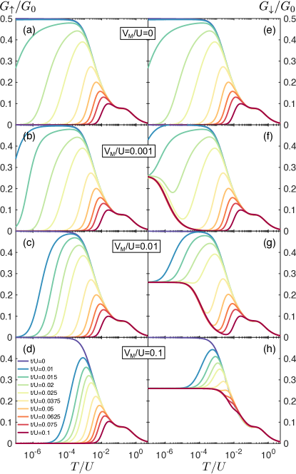
Figure 8: The temperature dependence of the linear-response spin-resolved conductance through the double dot for (left column) spin-up and (right column) spin-down components calculated for different values of the hopping $t$ between the dots and the coupling to the Majorana wire $V_{M}$, as indicated. The other parameters are the same as in Fig. 3.

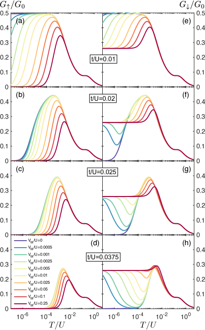
Figure 9: The same as in Fig. 8, now plotted for selected values of the hopping between the dots $t$, while changing the coupling to the Majorana wire $V_{M}$.

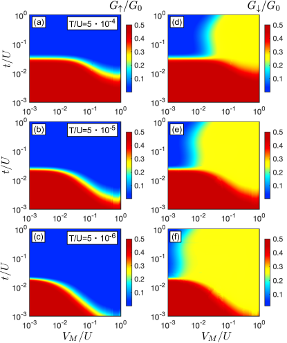
Figure 10: The linear-response conductance calculated as a function of the hopping between the dots $t$ and the coupling to the Majorana wire $V_{M}$ for different temperatures, as indicated. The left (right) column presents the spin-up (spin-down) contribution. The other parameters are the same as in Fig. 3. Note the logarithmic scale for both $t$ and $V_{M}$.

While the dependence of conductance on temperature for $T\gtrsim T_{K}$ is almost the same for different values of $t$ and $V_{M}$ (for the range of parameters considered in Figs. 8 and 9), the behavior of low-temperature conductance is completely different. Figure 10 presents the linear-response conductance for both spin components calculated at different temperatures while tuning both $t$ and $V_{M}$. Consider first the spin-up conductance for low-values of $V_{M}$, see the left column of Fig. 10. By increasing the hopping between the dots, the second-stage Kondo temperature becomes enhanced, such that when $T^{*}\gtrsim T$, $G_{\uparrow}$ drops from $(1/2)G_{0}$ to $0$. Thus, the point when this drop is observed is slightly different in each panel due to a different value of temperature $T$. When the coupling to Majorana wire increases, so does the second-stage Kondo temperature $T^{*}$, such that the conductance drop is observed for smaller values of $t$. In an extreme situation of very large $V_{M}$, if the temperature is sufficiently low, for all considered values of $t$ one has $T<T^{*}$, such that the conductance stays suppressed due to the second-stage Kondo effect, see Fig. 10(c) for $V_{M}\gtrsim U/10$. A somewhat similar behavior can be observed in the spin-down conductance component as far as the regions where $G_{\uparrow}=(1/2)G_{0}$ are concerned, see Fig. 10. This is due to the fact that when the hopping between the two dots is low, such that the second-stage Kondo effect does not develop, the influence of the coupling to the Majorana wire is rather negligible since the Majorana wire is coupled directly only to the second quantum dot. It is therefore clear that the influence of presence of Majorana mode will be most revealed in the parameter regime where the system exhibits the two-stage Kondo effect. Consequently, one observes a completely different behavior in the parameter space where $G_{\uparrow}\approx 0$, cf. the left and right column of Fig. 10. As can be clearly seen, with increasing $V_{M}$, there is a value of $V_{M}$ at which the conductance increases from $0$ to $(1/4)G_{0}$. At lower temperatures, smaller values of $V_{M}$ result in the corresponding change of conductance, which is due to the fact that the condition $\Gamma_{M}\gtrsim T$ can be satisfied for smaller values of $V_{M}$.

IV.2.2 Gate voltage dependence

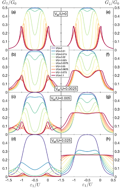
Figure 11: The conductance plotted as a function of the position of the first quantum dot level $\varepsilon_{1}$ for $\varepsilon_{2}=-U/2$ and for selected values the coupling to Majorana mode $V_{M}$, while changing the hopping between the dots $t$. The other parameters are the same as in Fig. 3 with $T=10^{-6}D$.

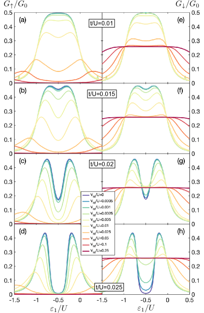
Figure 12: The same as in Fig. 10, now plotted for selected values of hopping between the dots $t$, while changing the coupling to Majorana mode $V_{M}$.

Let us now discuss the gate voltage dependence of the linear-response conductance. In the following we consider the case when the level of the first quantum dot is tuned, while the level of the second dot is at half filling. The spin-resolved conductance as a function of $\varepsilon_{1}$ calculated for selected values of both $t$ and $V_{M}$ at extremely low yet non-zero temperature $T=10^{-6}U$ is shown in Figs. 11 and 12. Both spin-up and spin-down conductances exhibit the Kondo plateau for small values of $t$ and $V_{M}$ in the transport regime where the first dot is singly occupied. When the hopping between the dots increases, for $V_{M}=0$, the Kondo plateau becomes distorted and the conductance suppression develops due to the two-stage Kondo effect, see Fig. 11(a). This suppression becomes more effective when the coupling to Majorana wire is turned on, however, then a clear difference between the spin components shows up. In the spin-up channel, increasing $t$ and/or $V_{M}$, generally results in larger suppression of the conductance in the singly-occupied first dot regime, i.e. for $-U\lesssim\varepsilon_{1}\lesssim 0$. This is related to the corresponding increase of $T^{*}$, as already discussed in previous sections. Similarly to the case $\varepsilon_{1}=\varepsilon_{2}=-U/2$ considered so far, also for other values of $\varepsilon_{1}$ finite coupling to the Majorana wire enhances $T^{*}$ and can suppress the conductance through the system; see e.g.Fig. 12(a)

On the other hand, in the case of spin-down conductance one can see that once the second-stage Kondo effect comes into play in the spin-up channel, i.e. suppression of conductance takes place, $G_{\downarrow}$ reaches a fractional value of $(1/4)G_{0}$. This is a direct fingerprint of the leakage of Majorana quasiparticle into the double-dot structure. Consequently, with increasing $V_{M}$, the total conductance saturates at $(1/4)G_{0}$. Moreover, when the coupling to the Majorana wire grows further, this value becomes stabilized in the whole region of the gate voltage and the conductance hardly depends on the occupation of the first quantum dot. Similar effect has been predicted for single dots coupled to Majorana wire Lee et al. (2013); Ruiz-Tijerina et al. (2015); Weymann and Wójcik (2017); Górski et al. (2018). Here, we demonstrate that the Majorana zero-energy mode can leak through the dot directly coupled to topological superconductor further into the nanostructure, and give rise to fractional values of conductance.

IV.3 Short Majorana wire case

The interplay between the Majorana and Kondo correlations described in the previous sections can be greatly affected in the case of relatively short topological superconducting wires. Then, a finite overlap between the wave functions of the two Majorana quasiparticles $\gamma_{1}$ and $\gamma_{2}$, described by $\varepsilon_{M}$, can emerge. As shown in the following, such overlap has a strong influence on the quantum interference responsible for fractional values of the conductance. In fact, such a strong dependence has already been reported theoretically in the case of single quantum dots coupled to external contacts and to the Majorana wire Lee et al. (2013); López et al. (2014); Weymann (2017); Weymann and Wójcik (2017). To examine the influence of the overlap $\varepsilon_{M}$ on the transport behavior of the considered double-dot-Majorana setup, in Fig. 13 we show the energy dependence of the spin-resolved spectral function, while Fig. 14 presents the temperature dependence of the linear conductance through the system. These figures were plotted based on calculations performed for selected values of $\varepsilon_{M}$ while changing the hopping between the dots and for fixed coupling to Majorana wire, $V_{M}/U=0.01$. The two figures are complementary in the sense that the temperature dependence of the conductance basically resembles the behavior of the spectral function, except for the fact that some features are smeared out by thermal fluctuations. The case of $\varepsilon_{M}=0$ presented in the first row of Figs. 13 and 14 is just for reference, to help identifying the impact of finite overlap on the behavior of $A_{\sigma}(\omega)$ and $G_{\sigma}$.

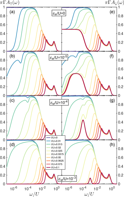
Figure 13: The normalized spectral function $\pi\Gamma A_{\sigma}(\omega)$ for the spin-up (left column) and spin-down (right column) components calculated for different values of the overlap between the Majorana zero-energy modes $\varepsilon_{M}$ and the hopping $t$ between the two dots, as indicated. The parameters are the same as in Fig. 3 with $V_{M}/U=0.01$.

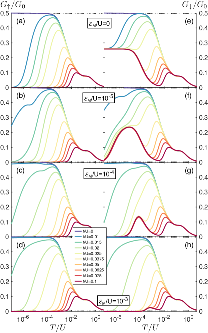
Figure 14: The linear-response conductance calculated as a function of temperature for different values of the overlap $\varepsilon_{M}$ and the hopping between the dots $t$, as indicated. The left (right) column presents the spin-up (spin-down) component. The parameters are the same as in Fig. 3 with $V_{M}/U=0.01$.

The influence of $\varepsilon_{M}$ on the spin-up component can be observed in the left column of Figs. 13 and 14. A small local minimum can be seen at the energy scale corresponding to $\varepsilon_{M}$. Interestingly, below this energy scale the interference with the Majorana mode becomes suppressed and the behavior of both $A_{\uparrow}(\omega)$ and $G_{\uparrow}$ starts resembling that in the case of $V_{M}=0$. This is especially visible for $\varepsilon_{M}/U=10^{-3}$, which is presented in Figs. 13(d) and 14(d), where the dependence of the quantities of interest is very similar to that depicted in Figs. 3(a) and 8(a), respectively. Note also that this apparent switching off of the Majorana leakage may lead to additional nonmonotonic behavior of the relevant spectral function if the energy scales happen to fulfill $T^{*}(V_{M}=0)<\varepsilon_{M}<T^{*}(V_{M})$; see e.g. the curve for $t=0.01U$ in Fig. 14(b).

The destructive influence of the overlap $\varepsilon_{M}$ on the quantum interference with Majorana mode is also visible in the spin-down component of both the spectral function and the conductance, which are presented in the right columns of Figs. 13 and 14. Now, a local minimum at the energy scale of $\varepsilon_{M}$ can also be observed, see e.g. the case for $\varepsilon_{M}/U=10^{-5}$. Moreover, below this energy scale the behavior of $A_{\downarrow}(\omega)$ and $G_{\downarrow}$ becomes comparable to that in the case of $V_{M}=0$, i.e. the conductance becomes fully suppressed for large $t$ and $T\lesssim\varepsilon_{M}$. If the overlap is increased further, see the case of $\varepsilon_{M}/U=10^{-3}$, the behavior of transport quantities resembles that in the absence of coupling to the Majorana wire, except for an additional local maximum visible in both $A_{\downarrow}(\omega)$ and $G_{\downarrow}$ at the energy scale corresponding to $\varepsilon_{M}$. This result suggest that even strongly overlapping Majorana mode may partially leak into the attached quantum dot.

IV.4 Majorana wire coupled to both spins

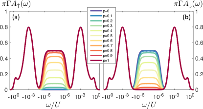
Figure 15: The normalized spectral function $\pi\Gamma A_{\sigma}(\omega)$ for (a) the spin-up and (b) spin-down components calculated for different values of the spin polarization $p$ of the Majorana modes, as indicated. The parameters are the same as in Fig. 3 with $V_{M}/U=0.001$ and $t/U=0.025$.

Finally, in this section we analyze the case when the Majorana quasiparticle couples to both spin projections of the double dot. We thus assume that there is a finite spin polarization of Majorana modes $p$ and express the double dot-Majorana coupling, cf. Eq. (5), as Górski et al. (2018), $\sum_{\sigma}V_{M\sigma}(d^{\dagger}_{2\sigma}-d_{2\sigma})(f^{\dagger}+f)$, where $V_{M\downarrow}=(1-p)V_{M}$ and $V_{M\uparrow}=pV_{M}$.

The spin-resolved spectral functions calculated for different values of polarization parameter $p$ are shown in Fig. 15. This figure clearly illustrates the five-peak structure in the behavior of the spectral function. The case of $p=0$ corresponds to no spin polarization of Majorana quasiparticles—the Majorana wire couples only to spin-down electrons. On the other hand, the case of $p=1$ corresponds to the situation when Majorana modes are coupled only to spin-up electrons in the double dot. One can see that now the spin-up spectral functions exhibits all the features discussed previously for $A_{\downarrow}(\omega)$. When the spin polarization increases from $p=0$ to $p=1$, the peak at the Fermi energy due to quantum interference with Majorana mode is continuously transferred between the two spin components, such that for $0<p<1$, the five-peak structure is visible in both spin-resolved spectral functions. Note, however, that the total spectral function, and consequently the total conductance, does not depend on $p$.

V Summary

In this paper we have examined the transport behavior of a double quantum dot in a T-shaped geometry, side-attached to a topological superconducting wire hosting Majorana zero-energy modes. The considerations were performed by using the numerical renormalization group method, which allowed us to accurately determine the behavior of the spin-resolved spectral functions and the linear-response conductance of the system. We have focused on the transport regime where the system exhibits the two-stage Kondo effect and investigated the influence of the coupling to Majorana wire on this Kondo phenomenon, considering both long and short Majorana wire cases. In the former case, the quantum interference with the Majorana quasiparticle gives rise to a half-suppression of the second-stage of Kondo effect, which results in a fractional value of the low-temperature conductance $G=(1/4)G_{0}$, where $G_{0}=2e^{2}/h$. This phenomenon develops at a new energy scale $\Gamma_{M}\propto V_{M}^{2}$ associated with the coupling to Majorana wire described by hopping amplitude $V_{M}$. We have shown that the Majorana-Kondo interplay can give rise to an additional resonance in the local density of states for energies lower than the Majorana scale $\Gamma_{M}$. This can be interpreted as a Majorana mode leaking further into the nanostructure, for it determines the low-temperature spectral properties of the first quantum dot, while the Majorana wire is coupled to the second quantum dot. At the same time, spectral density of the second dot is reduced by a half, proving that both dots can exhibit signatures of the Majorana physics at the same time. On the other hand, when there is an energy splitting $\varepsilon_{M}$ of Majorana modes due to a finite overlap of their wave functions, the quantum interference becomes suppressed and the system exhibits the usual two-stage Kondo effect for energies smaller than $\varepsilon_{M}$. Interestingly, both the conductance and spectral function exhibit a local maximum at the energy scale corresponding to $\varepsilon_{M}$.

Our findings demonstrate that the low-temperature transport behavior of T-shaped double quantum dots attached to Majorana wires exhibits some unique features due to the leakage of Majorana quasiparticles into the double dot system. First of all, fractional values of the conductance develop in the Majorana-Kondo regime. Moreover, the presence of topological superconductor increases the second-stage Kondo temperature through subtle renormalization effects, even though the relevant local exchange interaction is reduced. On the other hand, in the case of relatively short wires, a local maximum develops in the conductance for temperatures corresponding to the overlap between the two Majorana zero-energy modes. These signatures provide further examples of unique transport behavior due to the presence of Majorana zero-energy modes.

We would also like to notice that in the case of considered double quantum dot system the presence of Majorana quasiparticles results in a huge relative change of the low-temperature linear conductance [$G$ increases from $0$ to $(1/4)G_{0}$], opposite to single dots where the relative change is much smaller [$G$ drops from $G_{0}$ to $(3/4)G_{0}$]. The fractional conductance through T-shaped double quantum dot may thus serve as another important fingerprint of the presence of Majorana zero-energy modes in the system.

Finally, a comment on the intricate interplay of the three relevant energy scales determining the transport behavior, i.e. the coupling to topological wire $V_{M}$, the effective exchange interaction $J_{\rm eff}$ between the dots and the second-stage Kondo temperature $T^{*}$, is due. Despite the fact that $V_{M}$ slightly decreases the bare exchange interaction between the quantum dots, accurate numerical analysis has revealed an enhancement of the second-stage Kondo temperature. This tendency may seem natural if one accepts the fact that finite $V_{M}$ facilitates the development of the Kondo effect in the single quantum dot case Lee et al. (2013); Ruiz-Tijerina et al. (2015); Weymann and Wójcik (2017), however, it could not be inferred from perturbative analysis. It is thus not possible to a priori determine the fate of $T^{*}$, in particular to know if this effect is sufficient to overcompensate for the reduction of $J_{\rm eff}$ without numerical analysis. Actually, only after careful and extensive examination of the system’s parameter space have we concluded that the tendency for increase of $T^{*}$ with $V_{M}$ is indeed always the case. However, the precise explanation why this is so needs further examination.