Turbulent kinetic energy transport in oscillatory pipe flow

1 Introduction

Laminar as well as turbulent oscillatory pipe flows occur in many fields of biomedical science and engineering. Pulmonary air flow and vascular blood flow are usually laminar, because shear forces acting on the physiological system ought to be small. However, frictional losses and shear stresses vary considerably with transition to turbulence. This plays an important role in cases of e.g. artificial respiration or stenosis. On the other hand, in piston engines and reciprocating thermal/chemical process devices, turbulent or transitional oscillatory flows affect mixing properties, and also mass and heat transfer. In contrast to the extensively investigated statistically steady wall bounded shear flows, rather little work has been devoted to the onset, amplification and decay of turbulence in pipe flows driven by an unsteady external force. Experiments hino1976 ; eckmann1991 ; zhao1996 indicate that transition to turbulence depends on only one parameter, i.e. $Re_{\delta}\sim Re/W\!o$ with a critical value of about $550$, at least for Womersley numbers $W\!o>7$. We perform direct numerical simulations (DNS) of oscillatory pipe flows at several combinations of $Re$ and $W\!o$ to extend the validity of this critical value to higher $W\!o$. To better understand the physical mechanisms involved during decay and amplification of the turbulent flow, we further analyse the turbulent kinetic energy distribution and its budgets terms.

2 Numerical approach

We consider a Newtonian fluid confined by a straight pipe of diameter $D$ and length $L$. The fluid is driven in axial direction ($z$) by the time dependent pressure gradient

$$\textstyle\vec{P}(t)\equiv\left[0,0,\partial_{z}\langle p\rangle_{\phi}\right]^{\intercal}=\left[0,0,-4\cos\!\!\left(\frac{4W\!o^{2}}{Re_{\tau}}t\right)\right]^{\intercal}\text{, where}\hskip 9.95845ptp=p^{\prime}+\langle p\rangle_{\phi}$$ (1)

according to Reynolds’ decomposition. Prime denotes the fluctuating part and angle brackets the mean quantity averaged over equal oscillation phases. Normalisation and the set of non-dimensional control parameters is given by the Womersley number $W\!o=D/2\sqrt{\omega/\nu}$ and the friction Reynolds number $Re_{\tau}=u_{\tau}D/\nu$. Here, $\omega=2\pi/T$ is the forcing frequency, $\nu$ the kinematic viscosity, and $u_{\tau}$ the friction velocity of a fully developed statistically steady turbulent pipe flow. Thus, the governing equations read

$$\textstyle\vec{\begin{sideways}\begin{sideways}$\Delta$\end{sideways}\end{sideways}}\cdot\vec{u}=0\hskip 21.33955pt\text{and}\hskip 21.33955pt\partial_{t}\vec{u}+\left(\vec{u}\cdot\vec{\begin{sideways}\begin{sideways}$\Delta$\end{sideways}\end{sideways}}\right)\vec{u}+\vec{\begin{sideways}\begin{sideways}$\Delta$\end{sideways}\end{sideways}}p^{\prime}-\frac{1}{Re_{\tau}}{\boldsymbol{\Delta}}\vec{u}=\vec{P(t)}$$ (2)

with $\vec{u}$ denoting the velocity vector, $\partial_{t}$ being the partial derivative with respect to time $t$ and $\vec{\begin{sideways}\begin{sideways}$\Delta$\end{sideways}\end{sideways}}$ and ${\boldsymbol{\Delta}}$ being the Nabla operator and the Laplacian, respectively. Eqs. (1) and (2) are supplemented by periodic boundary conditions (BC) for $\vec{u}$ and $p$ in the homogeneous directions $z$ and $\varphi$ and no-slip and impermeability BC at $r=D/2$ in the radial direction. They are directly solved by means of a fourth order accurate finite volume method and advanced in time using a second order accurate leapfrog–Euler time integration scheme. Further details on the numerical method are given in Feldmann & Wagner feldmann2012 and references therein. The initial flow field was taken from a well correlated statistically steady turbulent pipe flow at $Re_{\tau}=1440$ discussed in feldmann2012 . The criterion $\overline{h}^{*}<\pi(Re_{\delta}/\langle k^{*}_{\epsilon}\rangle_{z,\varphi,\phi})^{1/4}$ for the mean grid size leads to $\overline{h}^{*}=\{6.2;7.1;5.7\}$ for cases I to III based on the maximum turbulent dissipation rates plotted in fig. 3. Since the mean grid spacing varies from the wall to the axis between $0.6<\overline{h}^{*}<1.0$, $1.3<\overline{h}^{*}<2.2$, and $0.6<\overline{h}^{*}<1.1$, respectively, we conclude, that the used grids are sufficiently fine to resolve all relevant length scales.

3 Computational parameters and flow regimes

We focus on DNS results obtained for three combinations of $W\!o=\left\{13,26,52\right\}$ and $Re_{\tau}=\left\{1440,5760,11520\right\}$, resulting in different peak Reynolds numbers $Re=\hat{u}D/\nu$ based on the maximum value of the respective bulk velocity $\langle\bar{u}(t)\rangle_{\phi}$ within $0<t\leq T$. Here, $\phi$ symbolises averaging over $N=14$ equal phases with $t+nT/2$ for $n=\{n\in\mathbb{N}:n\leqslant N\}$. The resulting parameter space in terms of $Re$ and $W\!o$ is shown in fig. 1, where $Re_{\delta}=\delta\hat{u}/\nu=Re/W\!o\sqrt{1/2}$ is the Reynolds number based on the Stokes layer thickness $\delta=\sqrt{2\nu/\omega}$.

[width=0.60]103_criticalParametersDles2013paper-eps-converted-to.pdf

Figure 1: Non-dimensional parameter space and flow regimes in terms of $Re$ and $W\!o$. Circles denote laminarised flows and squares turbulent flows. Here, we focus on the turbulent cases I, II, and III. Transition from laminar to the turbulent flow regime is indicated by the green hino1976 , red zhao1996 , and orange eckmann1991 lines as obtained experimentally. The blue line trukenmueller2006 separates regions of stability according to a quasi-steady stability analysis.

All flows denoted by circles laminarise despite of high $Re$ up to $\sim 12000$. The stabilising effect of the oscillatory forcing increases with $W\!o$, at least beyond a certain value of about seven, in agreement with findings from stability analysis trukenmueller2006 and experimental investigations hino1976 ; zhao1996 ; eckmann1991 .

Fig. 2 presents time series of the applied forcing $\vec{P}(t)$, the predicted mean shear stress at the wall $\langle\tau^{*}_{w}\rangle_{z,\varphi}$, and the axial velocity component $u_{z}(r,t)$ close to the wall ($r/D=0.49$) and near the center line ($r/D=0.01$).

[width=0.33]103_uProbeOsciPipe0034dles2013paper-eps-converted-to.pdf

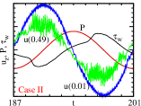
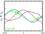
Figure 2: Time series of the axial velocity component $u_{z}(r,t)$ close to the wall at $r/D=0.49$ and close to the centre line at $r/D=0.01$, the forcing $\vec{P}(t)$, and the mean wall shear stress $\langle\tau^{*}_{w}\rangle_{z,\varphi}$.

The time series of $u_{z}$ reveal conditionally turbulent flows for all three parameter combinations, i.e. case I at $W\!o=13$ and $Re=11460$, case II at $W\!o=26$ and $Re=48175$, and case III at $W\!o=52$ and $Re=48250$, respectively. For I and III, i.e. the two slightly supercritical cases both at $Re_{\delta}\sim 600$, the near wall velocity characteristics are similar. Fluctuations suddenly grow only at deceleration (DC), while they are damped again during flow reversal (RV) and the following acceleration (AC) phase. These turbulent bursts during DC are also reflected in the $\tau^{*}_{w}$ history. However, the most conspicuous difference between I (lower $W\!o$) and III (higher $W\!o$) in this respect is that the AC phase is more stable for $W\!o=13$ despite of the similar $Re_{\delta}$, while fluctuations in the near wall flow do not completely decay for higher $W\!o$. Contrarily, the $u_{z}$ history at the centre line is completely smooth for case III, while for case I the core region is characterised by substantial velocity fluctuations throughout the whole oscillation cycle.

For higher values of $Re_{\delta}$, i.e. case II, the velocity time series reveal a completely different behaviour without distinct bursts and strong velocity fluctuations at the centre line. The turbulence intensity close to the wall and in the core region rather increases during AC and decreases during DC analogously to the bulk flow with laminarisation only during RV.

4 Turbulent kinetic energy

To shed light on the mechanisms leading to the different behaviour in decay and amplification of turbulence in the oscillatory pipe flows discussed above, we analyse the turbulent kinetic energy $k^{*}$ as well as the production and dissipation terms of its transport equation, see e.g. feldmann2012 . During all oscillation phases, both flows at $Re_{\delta}\sim$600$$ develop a boundary layer with one major characteristic, which is typical for wall-bounded shear flows. The turbulent kinetic energy profiles exhibit an obvious maximum very close to the wall with a very steep decrease towards the wall ($r^{*}=0$) and a moderate drop towards the pipe centre line. This can be seen from the radial $k^{*}$ distribution for I and III, shown in fig. 3.

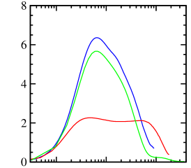
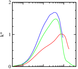
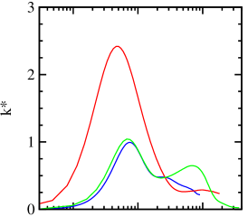
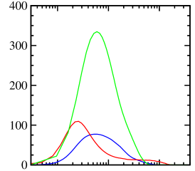
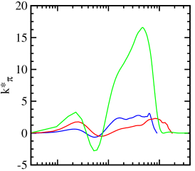
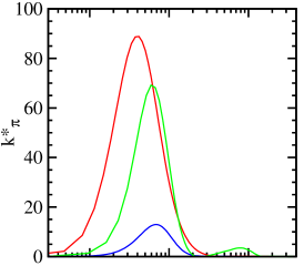
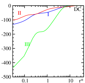
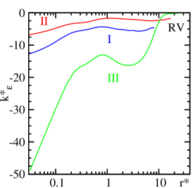
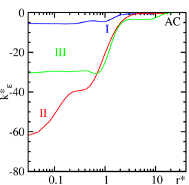
Figure 3: Radial distribution of turbulent kinetic energy $k^{*}$, its production term $k^{*}_{\pi}$, and its turbulent dissipation term $k^{*}_{\epsilon}$ scaled in Stokes layer thicknesses during DC, RV, and AC for I: $W\!o=13$, $Re_{\delta}=623$; II: $W\!o=26$, $Re_{\delta}=1310$; and III: $W\!o=52$, $Re_{\delta}=656$.

They reach the same maximum value for similar $Re_{\delta}$ and thus the ratio of $Re$ to $W\!o$ is the governing parameter defining equally turbulent oscillatory pipe flows. However, due to the shorter oscillation phase in case III, i.e. a four times higher $W\!o$, the same amount of energy is produced in a shorter period of time, as reflected by the four times higher production rate $k_{\pi}$ presented in fig. 3. For I and III, the turbulent kinetic energy monotonically decays from DC via RV even until AC. The production term $k^{*}_{\pi}$ further confirms, that turbulence is mostly generated when turbulent near-wall bursts occur during DC, cf. fig. 2. During RV, more energy is dissipated than produced at a dissipation rate $k^{*}_{\pi}$ even higher as during AC. Furthermore, for $Re_{\delta}\sim 600$ the $k^{*}_{\pi}$ profile becomes negative in a small annular region, where turbulent kinetic energy is transferred back to the mean flow, see also feldmann2012 . Both phenomena in combination account for the rigorous laminarisation during RV.

In contrast, for $Re_{\delta}=1310$ the turbulent kinetic energy decreases to the half during RV and increases again during AC to about the same value as in DC, due to the highest production rate $k^{*}_{\pi}$ during AC. Case II is also different in such a way that the turbulent kinetic energy is also rather high in most of the core region during DC, characterised by a flat broad $k^{*}$ profile only showing a vague near-wall maximum. While during AC the $k^{*}$ distribution clearly exhibits the above described typical shear flow profile. The same typical shear flow behaviour is reflected by the $k^{*}_{\epsilon}$ distribution with a maximum dissipation at the wall and a distinct plateau during all oscillation phases for $Re_{\delta}=1310$. The slightly supercritical cases I and III at $Re_{\delta}\sim 600$, on the other hand, develop a second local dissipation maximum, which becomes more pronounced in the $k^{*}_{\epsilon}$ profiles with ongoing laminarisation during RV and AC.

The wall distance $r^{*}=\left(1/2-r\right)D/\delta$ of the $k^{*}$ maxima are also the same for similar $Re_{\delta}$, when the length is scaled in Stokes layer thicknesses $\delta$. During DC and AC, when the bulk flow is high, the $k^{*}$ maximum occurs closer to the wall for higher $Re_{\delta}$. Vice versa, the energy maximum occurs closer to the wall for lower $Re_{\delta}$ during RV, when viscous effects dominate. Thus, the ratio of $Re$ to $W\!o$ defines the thickness of the annular region in terms of $\delta$, in which the oscillatory pipe flow exhibits turbulent features, even though the thickness of this turbulent boundary layer is strongly phase dependent. Also the budget terms shown in fig. 3, reveal that the wall distance of all the characteristics in the profiles, i.e. maxima, inflection points, plateaus and so on, scale with $Re_{\delta}$. However, for decreasing $W\!o$ per definition the Stokes layer becomes large compared to the pipe radius and thus the geometrical constraint of the pipe wall gains importance. In case I turbulent near-wall structures evolve during DC and RV, penetrate farther towards the centre line, and thus span almost the whole core region, cf. fig. 2. As a result, the turbulent kinetic energy is rather high over most parts of the pipe radius and, more important, does not vanish at the pipe axis for lower $W\!o$. Whereas, in case III at higher $W\!o$ but equal $Re_{\delta}$ the $k^{*}$ distribution reflect a high turbulent kinetic energy for $r^{*}<9$ and an almost laminar flow over the second half of the pipe radius. As indicated before by the velocity time series shown in fig. 2, the turbulence is confined to a smaller (in terms of $r$) annular region close to the wall, while the flow remains very smooth in the whole core region for the highest $W\!o$. The contribution of all other transport terms, i.e. the viscous, turbulent, and pressure diffusion as well as the pressure strain, to the overall budget is much lower. In principle, these terms reflect the typical shear flow mechanisms, which are simply damped and amplified by the oscillatory forcing, and thus for the sake of brevity not further discussed here.

5 Conclusions

Decay, amplification, and redistribution of turbulent kinetic energy in oscillatory pipe flow were studied by means of DNS for various combinations of $Re$ and $W\!o$. We found, that oscillatory flows at $Re_{\delta}<550$ relaminarise when started from a fully developed turbulent flow field despite of high $Re$. In very good agreement with experiments hino1976 ; eckmann1991 ; zhao1996 , we confirm oscillatory flows at $Re_{\delta}>550$ to be conditionally turbulent. However, we contradict eckmann1991 who stated that core flow remains stable for $Re_{\delta}<1310$. Our DNS results extend the validity of this experimentally determined critical value up to $W\!o=52$ in the $Re$-$W\!o$-space. Nevertheless, from the analysed turbulent kinetic energy distributions we conclude that decay and amplification of turbulence in oscillatory pipe flows rather depend on the combination of $Re$ and $W\!o$ then on its ratio ($Re_{\delta}$) alone. This is a significant difference to the case for the oscillating boundary layer over a flat plate, which has been extensively studied by Spalart & Baldwin spalart1989 using DNS. Even if experiments have shown that, the transition to turbulence can be characterised by only using $Re_{\delta}$, at least for $W\!o>7$, our study revealed that for oscillatory pipe flow the additional geometrical constraint considerably affects the decay and amplification of turbulence in the core flow.

References

- (1) Eckmann, D.M., Grotberg, J.B.: Experiments on transition to turbulence in oscillatory pipe flow. J. Fluid Mech. 222, 329–350 (1991)
- (2) Feldmann, D., Wagner, C.: Direct numerical simulation of fully-developed turbulent and oscillatory pipe flows at . J. Turb. 13, 1–28 (2012)
- (3) Hino, M., Sawamoto, M., Takasu, S.: Experiments on transition to turbulence in an oscillatory pipe flow. J. Fluid Mech. 75, 193–207 (1976)
- (4) Spalart, P.R., Baldwin, B.S.: Direct simulation of a turbulent oscillating boundary layer. In: Andre, J.C. et al. (eds.) Turbulent Shear Flows 6, 417–440. Springer (1989)
- (5) Trukenmüller, K.E.: Stabilitätstheorie für die oszillierende Rohrströmung. PhD Thesis, Helmut–Schmidt–Universität, Hamburg (2006)
- (6) Zhao, T.S., Cheng, P.: Experimental studies on the onset of turbulence and frictional losses in an oscillatory turbulent pipe flow. Int. J. Heat Fluid Fl. 17, 356–362 (1996)