Adaptive refinement with locally linearly independent LR B-splines: Theory and applications111This work has received funding from the European Union’s Horizon 2020 Research and Innovation Programme (grant agreement No 675789) and from the MIUR Excellence Department Project awarded to the Department of Mathematics, University of Rome Tor Vergata (CUP E83C18000100006). The authors are members of Gruppo Nazionale per il Calcolo Scientifico, Istituto Nazionale di Alta Matematica.

Francesco Patrizi francesco.patrizi@sintef.no Carla Manni manni@mat.uniroma2.it Francesca Pelosi pelosi@mat.uniroma2.it Hendrik Speleers speleers@mat.uniroma2.it Department of Applied Mathematics and Cybernetics, SINTEF, Oslo, Norway Department of Mathematics, University of Oslo, Oslo, Norway Department of Mathematics, University of Rome Tor Vergata, Rome, Italy
Abstract

In this paper we describe an adaptive refinement strategy for LR B-splines. The presented strategy ensures, at each iteration, local linear independence of the obtained set of LR B-splines. This property is then exploited in two applications: the construction of efficient quasi-interpolation schemes and the numerical solution of elliptic problems using the isogeometric Galerkin method.

keywords:
Adaptive refinement , LR B-splines , local linear independence , quasi-interpolation , isogeometric analysis.
journal: TBA
\newfloatcommand

capbtabboxtable[][\FBwidth] \usetkzobjall

1 Introduction

Since the ’70s, curves and surfaces in engineering are usually expressed by means of computer aided design (CAD) technologies, such as B-splines and non-uniform rational B-splines (NURBS). Thanks to properties like nonnegativity, local support and partition of unity, they allow for an easy control and modification of the geometries they describe, and this motivates their undisputed success as main modeling tools for objects with complex shapes in engineering; see, e.g., [21, 7, 18] and references therein. On the other hand, B-splines also provide a very efficient representation of smooth piecewise polynomial spaces, and so are a popular ingredient in the construction of approximation schemes; see, e.g., [2, 22, 17] and references therein.

More recently, the advent of isogeometric analysis (IgA) has integrated spline and CAD technologies into finite element analysis (FEA); see, e.g., [8, 1]. IgA aims to unify the geometric description of the domain of the differential problem with its numerical resolution, in order to expedite the simulation process and gaining in accuracy. In addition to the properties listed above, B-splines and NURBS feature other qualities appreciated in this context, such as (local) linear independence and high global smoothness.

Tensor structures admit a simple but powerful multivariate extension of univariate splines and B-splines. On the other hand, they lack adequate local refinement. The constantly increasing demand for higher precision in simulations and reverse engineering processes requires the possibility to apply adaptive local refinement strategies, in order to reduce the approximation error while keeping the computational costs low. This request for adaptivity, triggered the interest in new formulations of B-splines and NURBS, still based on local tensor structures [12, 23, 9, 5, 13, 10, 11]. All these new classes of functions are defined on locally refined meshes, in which T-vertices in the interior of the domain are allowed, the so-called T-meshes.

Locally refined B-splines, or in short LR B-splines [10], are one of these new formulations, and their definition is inspired by the knot insertion refinement process of tensor B-splines. These latter are defined on global knot vectors, one per direction. The insertion of a new knot in a knot vector corresponds to a line segment in the mesh crossing the entire domain. This refines all the B-splines whose supports are crossed. Instead, LR B-splines are defined on local knot vectors and the insertion of a new knot is always performed with respect to a particular LR B-spline. As a consequence, the LR B-spline definition is consistent with the tensor B-spline definition when the underlying mesh at the end of the process is a tensor mesh, and the formulation of LR B-splines remains broadly similar to classical tensor B-splines even though they allow for local refinements. This makes them one of the most elegant extensions of univariate B-splines on local tensor structures.

LR B-splines possess almost all the properties of classical tensor B-splines. Unfortunately, they are not always linearly independent. To this day, it is not yet known what are the precise conditions on the locally refined mesh to ensure a linearly independent set of LR B-splines, but some progress has been made in this direction. In [10] an efficient algorithm to seek and destroy linear dependence relations has been introduced, but it does not handle every possible locally refined mesh. In [20] a first analysis on the necessary conditions for encountering a linear dependence relation has been presented. There, it has also been proved that, for any bidegree, a linear dependence relation in the LR B-spline set involves at least 8 functions. In [3, 4] a characterization of the local linear independence of LR B-splines has been provided. Such a strong property is guaranteed only on locally refined meshes with strong constraints on the lengths and positions of the line segments that yield particular arrangements of the LR B-spline supports. On the other hand, a practical adaptive refinement strategy to produce meshes with the local linear independence property is still missing in the literature. To the best of our knowledge, the only mesh construction that leads to a locally linearly independent set of LR B-splines can be found in [4]. Such a construction, however, cannot be considered as a practical strategy because the regions to be refined and the maximal resolution, i.e., the sizes of the smallest cells in the domain induced by the mesh, must be chosen a priori.

In this paper, we describe a practical refinement strategy ensuring the local linear independence of the corresponding LR B-splines. Such a property is appealing as it admits, e.g., the construction of efficient quasi-interpolation schemes and the unisolvency of linear systems obtained by isogeometric discretization of differential problems based on such LR-splines. The remainder of the paper is divided into 5 sections. Section 2 contains the definition of LR B-splines and a summary of their main properties, whereas Section 3 describes the mesh refinement strategy and is the core of the paper. Sections 4 and 5 present applications of the refinement strategy in the context of quasi-interpolation and isogeometric Galerkin discretizations of elliptic problems. We end in Section 6 with some concluding remarks.

Throughout the paper, we assume the reader to be familiar with the definition and main properties of (univariate) B-splines, in particular with the knot insertion procedure. An introduction to this topic can be found, e.g., in the review papers [18, 17] or in the classical books [2] and [22].

2 Locally refined B-splines

In this section, we introduce locally refined B-splines, or in short LR B-splines, and discuss several of their properties, following the terminology from [20]. We denote by ΠpsubscriptΠ𝑝\Pi_{p} the space of univariate polynomials of degree less than or equal to p𝑝p, and by Π𝒑subscriptΠ𝒑\Pi_{\boldsymbol{p}} the space of bivariate polynomials of degrees less than or equal to 𝒑=(p1,p2)𝒑subscript𝑝1subscript𝑝2\boldsymbol{p}=(p_{1},p_{2}) component-wise. Furthermore, we denote by B[𝒙,𝒚]𝐵𝒙𝒚B[\boldsymbol{x},\boldsymbol{y}] the bivariate B-spline defined on the (local) knot vectors 𝒙=(x1,,xp1+2)𝒙subscript𝑥1subscript𝑥subscript𝑝12\boldsymbol{x}=(x_{1},\ldots,x_{p_{1}+2}) and 𝒚=(y1,,yp2+2)𝒚subscript𝑦1subscript𝑦subscript𝑝22\boldsymbol{y}=(y_{1},\ldots,y_{p_{2}+2}), where xixi+1subscript𝑥𝑖subscript𝑥𝑖1x_{i}\leq x_{i+1} and yiyi+1subscript𝑦𝑖subscript𝑦𝑖1y_{i}\leq y_{i+1} for all i𝑖i. The bidegree of B[𝒙,𝒚]𝐵𝒙𝒚B[\boldsymbol{x},\boldsymbol{y}] is 𝒑=(p1,p2)𝒑subscript𝑝1subscript𝑝2\boldsymbol{p}=(p_{1},p_{2}) and is implicitly specified by the length of 𝒙𝒙\boldsymbol{x} and 𝒚𝒚\boldsymbol{y}.

In order to define LR B-splines, we first introduce the concept of box-partition.

Definition 2.1.

Given an axis-aligned rectangle Ω2Ωsuperscript2\Omega\subseteq{\mathbb{R}}^{2}, a box-partition of ΩΩ\Omega is a finite collection \mathcal{E} of axis-aligned rectangles in ΩΩ\Omega such that

  1. 1.

    β̊1β̊2=subscript̊𝛽1subscript̊𝛽2\mathring{\beta}_{1}\cap\mathring{\beta}_{2}=\emptyset for any β1,β2subscript𝛽1subscript𝛽2\beta_{1},\beta_{2}\in\mathcal{E}, with β1β2subscript𝛽1subscript𝛽2\beta_{1}\neq\beta_{2};

  2. 2.

    ββ=Ωsubscript𝛽𝛽Ω\bigcup_{\beta\in\mathcal{E}}\beta=\Omega.

Given a box-partition \mathcal{E}, we define the vertices of \mathcal{E} as the vertices of its elements. A meshline is an axis-aligned segment contained in an edge of an element of \mathcal{E}, connecting two and only two vertices of \mathcal{E} located at its end-points. The collection of all the meshlines of the box-partition is called mesh, and denoted by {\mathcal{M}}. A meshline can be expressed as the Cartesian product of a point in {\mathbb{R}} and a finite interval. Let α𝛼\alpha\in{\mathbb{R}} be the value of such a point and let k{1,2}𝑘12k\in\{1,2\} be its position in the Cartesian product. If k=1𝑘1k=1 the meshline is vertical and if k=2𝑘2k=2 the meshline is horizontal. We sometimes write k𝑘k-meshline to specify the direction of the meshline, and (k,α)𝑘𝛼(k,\alpha)-meshline to specify exactly on which axis-parallel line in 2superscript2{\mathbb{R}}^{2} the meshline lies. A vertex of \mathcal{E} is called T-vertex if it is the intersection of two collinear meshlines and another meshline, say γ𝛾\gamma, orthogonal to them. We call the T-vertex vertical if γ𝛾\gamma is vertical, and horizontal otherwise.

For defining splines of a certain bidegree 𝒑=(p1,p2)𝒑subscript𝑝1subscript𝑝2\boldsymbol{p}=(p_{1},p_{2}) and smoothness across the meshlines, we also need the notion of multiplicity of a meshline. This is a positive integer associated with every meshline in {\mathcal{M}}. For a k𝑘k-meshline this number is assumed to be maximally pk+1subscript𝑝𝑘1p_{k}+1. A meshline in {\mathcal{M}} has full multiplicity if its multiplicity is maximal, and we say that {\mathcal{M}} is open if every boundary meshline has full multiplicity. If all the meshlines of the box-partition have the same multiplicity m𝑚m we say that {\mathcal{M}} has multiplicity m𝑚m. When the T-vertices of \mathcal{E} occur only on ΩΩ\partial\Omega and all collinear meshlines have the same multiplicity, the corresponding mesh is called tensor mesh. Figure 1 shows an example of a box-partition and its associated mesh.

β1subscript𝛽1\beta_{1}β2subscript𝛽2\beta_{2}β3subscript𝛽3\beta_{3}β5subscript𝛽5\beta_{5}β4subscript𝛽4\beta_{4}β6subscript𝛽6\beta_{6}
(a)
111111111111111111333111222444222222111111111111111222
(b)
Figure 1: Example of a box-partition {\mathcal{E}} of a rectangle ΩΩ\Omega in (a), and the mesh corresponding to {\mathcal{E}} in (b). The meshlines are identified by squares showing the associated multiplicities.

Given a bivariate B-spline B[𝒙,𝒚]𝐵𝒙𝒚B[\boldsymbol{x},\boldsymbol{y}], let xi1,,xirsubscript𝑥subscript𝑖1subscript𝑥subscript𝑖𝑟x_{i_{1}},\ldots,x_{i_{r}} and yj1,,yjssubscript𝑦subscript𝑗1subscript𝑦subscript𝑗𝑠y_{j_{1}},\ldots,y_{j_{s}} be the distinct knots in 𝒙𝒙\boldsymbol{x} and 𝒚𝒚\boldsymbol{y}, respectively. The mesh

(𝒙,𝒚):={{xi}×[yjn,yjn+1]:=1,,r;n=1,,s1}{[xin,xin+1]×{yj}:=1,,s;n=1,,r1}assign𝒙𝒚conditional-setsubscript𝑥subscript𝑖subscript𝑦subscript𝑗𝑛subscript𝑦subscript𝑗𝑛1formulae-sequence1𝑟𝑛1𝑠1conditional-setsubscript𝑥subscript𝑖𝑛subscript𝑥subscript𝑖𝑛1subscript𝑦subscript𝑗formulae-sequence1𝑠𝑛1𝑟1\begin{split}{\mathcal{M}}(\boldsymbol{x},\boldsymbol{y}):=\{&\{x_{i_{\ell}}\}\times[y_{j_{n}},y_{j_{n+1}}]:\,\ell=1,\ldots,r;\,n=1,\ldots,s-1\}\,\\ &\cup\,\{[x_{i_{n}},x_{i_{n+1}}]\times\{y_{j_{\ell}}\}:\ell=1,\ldots,s;\,n=1,\ldots,r-1\}\end{split} (1)

is a tensor mesh in suppB[𝒙,𝒚]supp𝐵𝒙𝒚\text{supp}\,B[\boldsymbol{x},\boldsymbol{y}]. The multiplicities of the meshlines in (𝒙,𝒚)𝒙𝒚{\mathcal{M}}(\boldsymbol{x},\boldsymbol{y}) are given by the multiplicities of the knots of B[𝒙,𝒚]𝐵𝒙𝒚B[\boldsymbol{x},\boldsymbol{y}]. For instance, the (1,xi)1subscript𝑥subscript𝑖(1,x_{i_{\ell}})-meshlines {xi}×[yjn,yjn+1]subscript𝑥subscript𝑖subscript𝑦subscript𝑗𝑛subscript𝑦subscript𝑗𝑛1\{x_{i_{\ell}}\}\times[y_{j_{n}},y_{j_{n+1}}] for n=1,,s1𝑛1𝑠1n=1,\ldots,s-1 have all the same multiplicity equal to the multiplicity of xisubscript𝑥subscript𝑖x_{i_{\ell}} in 𝒙𝒙\boldsymbol{x}.

Definition 2.2.

Given a mesh {\mathcal{M}} and a B-spline B[𝐱,𝐲]𝐵𝐱𝐲B[\boldsymbol{x},\boldsymbol{y}], we say that B[𝐱,𝐲]𝐵𝐱𝐲B[\boldsymbol{x},\boldsymbol{y}] has support on {\mathcal{M}} if

  • 1.

    the meshlines in (𝒙,𝒚)𝒙𝒚{\mathcal{M}}(\boldsymbol{x},\boldsymbol{y}) can be obtained as unions of meshlines in {\mathcal{M}}, and

  • 2.

    their multiplicities are less than or equal to the multiplicities of the corresponding meshlines in {\mathcal{M}}.

Furthermore, we say that B[𝐱,𝐲]𝐵𝐱𝐲B[\boldsymbol{x},\boldsymbol{y}] has minimal support on {\mathcal{M}} if

  • 1.

    it has support on {\mathcal{M}},

  • 2.

    the multiplicities of the interior meshlines in (𝒙,𝒚)𝒙𝒚{\mathcal{M}}(\boldsymbol{x},\boldsymbol{y}) are equal to the multiplicities of the corresponding meshlines in {\mathcal{M}}, and

  • 3.

    there is no collection γ𝛾\gamma of collinear meshlines in \(𝒙,𝒚)\𝒙𝒚{\mathcal{M}}\backslash{\mathcal{M}}(\boldsymbol{x},\boldsymbol{y}) such that suppB[𝒙,𝒚]\γ\supp𝐵𝒙𝒚𝛾\text{supp}\,B[\boldsymbol{x},\boldsymbol{y}]\backslash\gamma is not connected.

Figure 2 shows examples of B-splines of bidegree (2,2)22(2,2) with support on a mesh of multiplicity 111. In particular, the B-splines in (b)–(c) have minimal support, whereas the support of the B-spline in (d) can be disconnected by the collection of meshlines γ𝛾\gamma, visualized by dashed lines in the figure.

(a)
(b)
(c)
(d)
Figure 2: Support of B-splines of bidegree (2,2)22(2,2) on a mesh {\mathcal{M}} of multiplicity 111. The mesh is shown in (a). The B-splines whose supports are depicted in (b) and (c) have minimal support on {\mathcal{M}}. The tensor meshes defined by the B-spline’s knots are highlighted with thicker lines. On the other hand, the B-spline in (d) does not have minimal support on {\mathcal{M}}: the collection of meshlines contained in the dashed line disconnects its support.

Given a mesh {\mathcal{M}} and a B-spline B[𝒙,𝒚]𝐵𝒙𝒚B[\boldsymbol{x},\boldsymbol{y}] with support in {\mathcal{M}}, assume that it does not have minimal support on {\mathcal{M}}. Then, there exists a collection of (k,α)𝑘𝛼(k,\alpha)-meshlines γ𝛾\gamma such that suppB[𝒙,𝒚]\γ\supp𝐵𝒙𝒚𝛾\text{supp}\,B[\boldsymbol{x},\boldsymbol{y}]\backslash\gamma is not connected and either γ𝛾\gamma is in \(𝒙,𝒚)\𝒙𝒚{\mathcal{M}}\backslash{\mathcal{M}}(\boldsymbol{x},\boldsymbol{y}) or γ(𝒙,𝒚)𝛾𝒙𝒚\gamma\subseteq{\mathcal{M}}(\boldsymbol{x},\boldsymbol{y}), i.e., α𝛼\alpha is an internal knot of 𝒙𝒙\boldsymbol{x} for k=1𝑘1k=1 or 𝒚𝒚\boldsymbol{y} for k=2𝑘2k=2, but its meshlines have lower multiplicities in (𝒙,𝒚)𝒙𝒚{\mathcal{M}}(\boldsymbol{x},\boldsymbol{y}) than in {\mathcal{M}}. Assume that the meshlines in γ𝛾\gamma have all the same multiplicity m𝑚m in {\mathcal{M}}. Denoting by μ(α)0𝜇𝛼0\mu(\alpha)\geq 0 the number of times α𝛼\alpha appears in the knot vector of B[𝒙,𝒚]𝐵𝒙𝒚B[\boldsymbol{x},\boldsymbol{y}] in the k𝑘k-th direction, then mμ(α)𝑚𝜇𝛼m-\mu(\alpha) is strictly positive as B[𝒙,𝒚]𝐵𝒙𝒚B[\boldsymbol{x},\boldsymbol{y}] has support, but not minimal support, on {\mathcal{M}}. One could consider such α𝛼\alpha as an extra knot, of multiplicity mμ(α)𝑚𝜇𝛼m-\mu(\alpha), with respect to the knot vector of B[𝒙,𝒚]𝐵𝒙𝒚B[\boldsymbol{x},\boldsymbol{y}] in the k𝑘k-th direction (in 𝒙𝒙\boldsymbol{x} if k=1𝑘1k=1 and in 𝒚𝒚\boldsymbol{y} if k=2𝑘2k=2), and perform knot insertion on B[𝒙,𝒚]𝐵𝒙𝒚B[\boldsymbol{x},\boldsymbol{y}]. If α𝛼\alpha was already a knot of B[𝒙,𝒚]𝐵𝒙𝒚B[\boldsymbol{x},\boldsymbol{y}], so μ(α)1𝜇𝛼1\mu(\alpha)\geq 1, this means rising its multiplicity by mμ(α)𝑚𝜇𝛼m-\mu(\alpha). The resulting generated B-splines will still have support on {\mathcal{M}} and eventually they will also have minimal support on {\mathcal{M}}. As an example, the collection γ𝛾\gamma highlighted with dashed lines in Figure 2(d) is made of (2,α)2𝛼(2,\alpha)-meshlines, for some α𝛼\alpha, of multiplicity 1. Such α𝛼\alpha can be inserted as new knot of multiplicity 1 in the knot vector in the y𝑦y-direction of the considered B-spline to refine it in two B-splines via knot insertion.

The LR B-splines are generated by means of the above procedure. We start by considering a coarse tensor mesh and we refine it by inserting collections of collinear meshlines, one at a time, of the same multiplicity. On the initial mesh we consider the standard tensor B-splines and whenever a B-spline in our collection has no longer minimal support during the mesh refinement process, we refine it by using the knot insertion procedure. The LR B-splines will be the final set of B-splines produced by this algorithm. In the following definitions we formalize this by describing the mesh refinement process in our framework.

Definition 2.3.

Given a box-partition \mathcal{E} and an axis-aligned segment γ𝛾\gamma, we say that γ𝛾\gamma traverses β𝛽\beta\in\mathcal{E} if γβ𝛾𝛽\gamma\subseteq\beta and the interior of β𝛽\beta is divided into two parts by γ𝛾\gamma, i.e., β\γ\𝛽𝛾\beta\backslash\gamma is not connected. A split is a finite union of contiguous and collinear axis-aligned segments γ=iγi𝛾subscript𝑖subscript𝛾𝑖\gamma=\cup_{i}\gamma_{i} such that every γisubscript𝛾𝑖\gamma_{i} either is a meshline of the box-partition or traverses some β𝛽\beta\in\mathcal{E}. A mesh {\mathcal{M}} has constant splits if each split in it is made of meshlines of the same multiplicity.

Like for meshlines, we sometimes write k𝑘k-split with k{1,2}𝑘12k\in\{1,2\} to specify the direction of the split or (k,α)𝑘𝛼(k,\alpha)-split to specify on what axis-parallel line in 2superscript2{\mathbb{R}}^{2} the split lies.

When a split γ𝛾\gamma is inserted in a box-partition \mathcal{E}, any traversed β𝛽\beta\in\mathcal{E} is replaced by the two subrectangles β1,β2subscript𝛽1subscript𝛽2\beta_{1},\beta_{2} given by the closures of the connected components of β\γ\𝛽𝛾\beta\backslash\gamma. The resulting new box-partition will be denoted by +γ𝛾\mathcal{E}+\gamma and its corresponding mesh by +γ𝛾{\mathcal{M}}+\gamma. We also assume that a positive integer μγsubscript𝜇𝛾\mu_{\gamma} has been assigned to any split γ𝛾\gamma. The multiplicities of the meshlines in (+γ)𝛾{\mathcal{M}}\cap({\mathcal{M}}+\gamma) and not contained in γ𝛾\gamma are unchanged. Contrarily, the multiplicities of the meshlines in γ𝛾\gamma that were already in {\mathcal{M}} are rised by μγsubscript𝜇𝛾\mu_{\gamma}, and the new meshlines in γ𝛾\gamma have multiplicity equal to μγsubscript𝜇𝛾\mu_{\gamma} on +γ𝛾{\mathcal{M}}+\gamma.

The LR B-splines are defined on a class of meshes with constant splits, called LR-meshes. Thus, from now on, we restrict our attention to meshes that have constant splits. In particular, we note that when refining a mesh {\mathcal{M}} by inserting a split γ𝛾\gamma, either γ𝛾\gamma is made solely of new meshlines or it is made solely of meshlines already on {\mathcal{M}}, in order for +γ𝛾{\mathcal{M}}+\gamma to have constant splits.

Definition 2.4.

Given a mesh {\mathcal{M}} with constant splits, a B-spline B[𝐱,𝐲]𝐵𝐱𝐲B[\boldsymbol{x},\boldsymbol{y}] with support on {\mathcal{M}} and a split γ𝛾\gamma, we say that γ𝛾\gamma traverses B[𝐱,𝐲]𝐵𝐱𝐲B[\boldsymbol{x},\boldsymbol{y}] if the interior of suppB[𝐱,𝐲]supp𝐵𝐱𝐲\text{supp}\,B[\boldsymbol{x},\boldsymbol{y}] is divided into two parts by γ𝛾\gamma, i.e., suppB[𝐱,𝐲]\γ\supp𝐵𝐱𝐲𝛾\text{supp}\,B[\boldsymbol{x},\boldsymbol{y}]\backslash\gamma is not connected and either γ𝛾\gamma is in \(𝐱,𝐲)\𝐱𝐲{\mathcal{M}}\backslash{\mathcal{M}}(\boldsymbol{x},\boldsymbol{y}) or γ(𝐱,𝐲)𝛾𝐱𝐲\gamma\subseteq{\mathcal{M}}(\boldsymbol{x},\boldsymbol{y}) but the multiplicity of its meshlines is lower in (𝐱,𝐲)𝐱𝐲{\mathcal{M}}(\boldsymbol{x},\boldsymbol{y}) than in {\mathcal{M}}.

We are now ready to define the mesh refinement process and the LR B-splines. The meshes generated by this procedure will be called LR-meshes.

Definition 2.5.

Given a bidegree 𝐩=(p1,p2)𝐩subscript𝑝1subscript𝑝2\boldsymbol{p}=(p_{1},p_{2}), let 1subscript1{\mathcal{M}}_{1} be a tensor mesh such that the set of standard tensor B-splines of bidegree 𝐩𝐩\boldsymbol{p} on 1subscript1{\mathcal{M}}_{1} is nonempty, and denote it by 1subscript1\mathcal{B}_{1}. We then define a sequence of meshes 2,3,subscript2subscript3{\mathcal{M}}_{2},{\mathcal{M}}_{3},\ldots and corresponding function sets 2,3,subscript2subscript3\mathcal{B}_{2},\mathcal{B}_{3},\ldots as follows. For i=1,2,𝑖12i=1,2,\ldots, let γisubscript𝛾𝑖\gamma_{i} be a split such that i+1:=i+γiassignsubscript𝑖1subscript𝑖subscript𝛾𝑖{\mathcal{M}}_{i+1}:={\mathcal{M}}_{i}+\gamma_{i} has constant splits and such that the support of at least one B-spline in isubscript𝑖{\mathcal{B}}_{i} is traversed by a split in i+1subscript𝑖1{\mathcal{M}}_{i+1}. On this refined mesh i+1subscript𝑖1{\mathcal{M}}_{i+1}, the new set of B-splines i+1subscript𝑖1{\mathcal{B}}_{i+1} is constructed by the following algorithm.

  1. 1.

    Initialize the set by i+1isubscript𝑖1subscript𝑖\mathcal{B}_{i+1}\leftarrow\mathcal{B}_{i}.

  2. 2.

    As long as there exists B[𝒙j,𝒚j]i+1𝐵superscript𝒙𝑗superscript𝒚𝑗subscript𝑖1B[\boldsymbol{x}^{j},\boldsymbol{y}^{j}]\in\mathcal{B}_{i+1} with no minimal support on i+1subscript𝑖1{\mathcal{M}}_{i+1}:

    1. (a)

      Apply knot insertion: B[𝒙1j,𝒚1j],B[𝒙2j,𝒚2j]:B[𝒙j,𝒚j]=α1B[𝒙1j,𝒚1j]+α2B[𝒙2j,𝒚2j]:𝐵superscriptsubscript𝒙1𝑗superscriptsubscript𝒚1𝑗𝐵superscriptsubscript𝒙2𝑗superscriptsubscript𝒚2𝑗𝐵superscript𝒙𝑗superscript𝒚𝑗subscript𝛼1𝐵superscriptsubscript𝒙1𝑗superscriptsubscript𝒚1𝑗subscript𝛼2𝐵superscriptsubscript𝒙2𝑗superscriptsubscript𝒚2𝑗\exists B[\boldsymbol{x}_{1}^{j},\boldsymbol{y}_{1}^{j}],B[\boldsymbol{x}_{2}^{j},\boldsymbol{y}_{2}^{j}]:B[\boldsymbol{x}^{j},\boldsymbol{y}^{j}]=\alpha_{1}B[\boldsymbol{x}_{1}^{j},\boldsymbol{y}_{1}^{j}]+\alpha_{2}B[\boldsymbol{x}_{2}^{j},\boldsymbol{y}_{2}^{j}].

    2. (b)

      Update the set: i+1(i+1\{B[𝒙j,𝒚j]}){B[𝒙1j,𝒚1j],B[𝒙2j,𝒚2j]}subscript𝑖1\subscript𝑖1𝐵superscript𝒙𝑗superscript𝒚𝑗𝐵superscriptsubscript𝒙1𝑗superscriptsubscript𝒚1𝑗𝐵superscriptsubscript𝒙2𝑗superscriptsubscript𝒚2𝑗\mathcal{B}_{i+1}\leftarrow(\mathcal{B}_{i+1}\backslash\{B[\boldsymbol{x}^{j},\boldsymbol{y}^{j}]\})\cup\{B[\boldsymbol{x}_{1}^{j},\boldsymbol{y}_{1}^{j}],B[\boldsymbol{x}_{2}^{j},\boldsymbol{y}_{2}^{j}]\}.

The mesh generated at each step is called LR-mesh and the corresponding function set is called LR B-spline set.

(a)
(b)
Figure 3: Two meshes. Assume that the boundary has a multiplicity large enough so that it is possible to define a B-spline of bidegree 𝒑𝒑\boldsymbol{p} on it. Then, the mesh in (a) is not an LR-mesh because it cannot be built as a sequence of split insertions. The mesh in (b) is an LR-mesh similar to the one in (a).

Obviously not every mesh is an LR-mesh. For instance, one could consider meshes that do not have constant splits or meshes that cannot be built through a sequence of split insertions as the mesh depicted in Figure 3(a). In general, the mesh refinement process producing a given LR-mesh =Nsubscript𝑁{\mathcal{M}}={\mathcal{M}}_{N} is not unique. Indeed, the split insertion ordering can often be changed. Nevertheless, the LR B-spline set on {\mathcal{M}} is well defined because it is independent of such insertion ordering, as proved in [10, Theorem 3.4].

Given an LR-mesh, the corresponding LR B-splines have several desirable properties for applications. By their definition, it is clear that

  • 1.

    they are nonnegative,

  • 2.

    they have minimal support, and

  • 3.

    they can be expressed by the LR B-splines on finer LR-meshes using nonnegative coefficients (provided by the knot insertion procedure).

Furthermore, it is possible to scale them by means of positive weights so that they also form a partition of unity; see [10, Section 7].

1234567891234567
(a)
720 =108 +135 +108 +324 +360 +108 +268 720 108 135 108 324 360 108 268 \begin{split}\hskip 85.35826pt\footnotesize{720}\cdot\raisebox{-8.00002pt}{ \leavevmode\hbox to45.92pt{\vbox to35.14pt{\pgfpicture\makeatletter\hbox{\hskip 0.2pt\lower-0.8pt\hbox to0.0pt{\pgfsys@beginscope\pgfsys@invoke{ }\definecolor{pgfstrokecolor}{rgb}{0,0,0}\pgfsys@color@rgb@stroke{0}{0}{0}\pgfsys@invoke{ }\pgfsys@color@rgb@fill{0}{0}{0}\pgfsys@invoke{ }\pgfsys@setlinewidth{0.4pt}\pgfsys@invoke{ }\nullfont\hbox to0.0pt{\pgfsys@beginscope\pgfsys@invoke{ }{}{{}}{} {}{} {}{} {}{} {}\pgfsys@beginscope\pgfsys@invoke{ }\definecolor[named]{pgfstrokecolor}{rgb}{1,0,0}\pgfsys@color@rgb@stroke{1}{0}{0}\pgfsys@invoke{ }\pgfsys@setlinewidth{1.6pt}\pgfsys@invoke{ }\definecolor{pgffillcolor}{rgb}{1,0.5,0.5}\pgfsys@color@rgb@fill{1}{0.5}{0.5}\pgfsys@invoke{ }{}\pgfsys@moveto{5.69046pt}{0.0pt}\pgfsys@lineto{39.83368pt}{0.0pt}\pgfsys@lineto{39.83368pt}{28.45276pt}\pgfsys@lineto{5.69046pt}{28.45276pt}\pgfsys@closepath\pgfsys@fillstroke\pgfsys@invoke{ } \pgfsys@invoke{\lxSVG@closescope }\pgfsys@endscope{}{{}}{} {}{}\pgfsys@beginscope\pgfsys@invoke{ }\color[rgb]{1,0,0}\definecolor[named]{pgfstrokecolor}{rgb}{1,0,0}\pgfsys@color@rgb@stroke{1}{0}{0}\pgfsys@invoke{ }\pgfsys@color@rgb@fill{1}{0}{0}\pgfsys@invoke{ }\definecolor[named]{pgffillcolor}{rgb}{1,0,0}\pgfsys@setlinewidth{1.6pt}\pgfsys@invoke{ }{}\pgfsys@moveto{5.69046pt}{5.69046pt}\pgfsys@lineto{39.83368pt}{5.69046pt}\pgfsys@stroke\pgfsys@invoke{ } \pgfsys@invoke{\lxSVG@closescope }\pgfsys@endscope{}{{}}{} {}{}\pgfsys@beginscope\pgfsys@invoke{ }\color[rgb]{1,0,0}\definecolor[named]{pgfstrokecolor}{rgb}{1,0,0}\pgfsys@color@rgb@stroke{1}{0}{0}\pgfsys@invoke{ }\pgfsys@color@rgb@fill{1}{0}{0}\pgfsys@invoke{ }\definecolor[named]{pgffillcolor}{rgb}{1,0,0}\pgfsys@setlinewidth{1.6pt}\pgfsys@invoke{ }{}\pgfsys@moveto{5.69046pt}{17.07182pt}\pgfsys@lineto{39.83368pt}{17.07182pt}\pgfsys@stroke\pgfsys@invoke{ } \pgfsys@invoke{\lxSVG@closescope }\pgfsys@endscope{}{{}}{} {}{}\pgfsys@beginscope\pgfsys@invoke{ }\color[rgb]{1,0,0}\definecolor[named]{pgfstrokecolor}{rgb}{1,0,0}\pgfsys@color@rgb@stroke{1}{0}{0}\pgfsys@invoke{ }\pgfsys@color@rgb@fill{1}{0}{0}\pgfsys@invoke{ }\definecolor[named]{pgffillcolor}{rgb}{1,0,0}\pgfsys@setlinewidth{1.6pt}\pgfsys@invoke{ }{}\pgfsys@moveto{11.38092pt}{0.0pt}\pgfsys@lineto{11.38092pt}{28.45276pt}\pgfsys@stroke\pgfsys@invoke{ } \pgfsys@invoke{\lxSVG@closescope }\pgfsys@endscope{}{{}}{} {}{}\pgfsys@beginscope\pgfsys@invoke{ }\color[rgb]{1,0,0}\definecolor[named]{pgfstrokecolor}{rgb}{1,0,0}\pgfsys@color@rgb@stroke{1}{0}{0}\pgfsys@invoke{ }\pgfsys@color@rgb@fill{1}{0}{0}\pgfsys@invoke{ }\definecolor[named]{pgffillcolor}{rgb}{1,0,0}\pgfsys@setlinewidth{1.6pt}\pgfsys@invoke{ }{}\pgfsys@moveto{28.45276pt}{0.0pt}\pgfsys@lineto{28.45276pt}{28.45276pt}\pgfsys@stroke\pgfsys@invoke{ } \pgfsys@invoke{\lxSVG@closescope }\pgfsys@endscope{}{{}}{} {}{} {}{} {}{} {}{}\pgfsys@moveto{0.0pt}{0.0pt}\pgfsys@lineto{45.52458pt}{0.0pt}\pgfsys@lineto{45.52458pt}{34.14322pt}\pgfsys@lineto{0.0pt}{34.14322pt}\pgfsys@closepath\pgfsys@stroke\pgfsys@invoke{ } {}{{}}{} {}{}{}\pgfsys@moveto{5.69046pt}{0.0pt}\pgfsys@lineto{5.69046pt}{34.14322pt}\pgfsys@stroke\pgfsys@invoke{ } {}{{}}{} {}{}{}\pgfsys@moveto{11.38092pt}{0.0pt}\pgfsys@lineto{11.38092pt}{34.14322pt}\pgfsys@stroke\pgfsys@invoke{ } {}{{}}{} {}{}{}\pgfsys@moveto{17.07182pt}{0.0pt}\pgfsys@lineto{17.07182pt}{22.76228pt}\pgfsys@stroke\pgfsys@invoke{ } {}{{}}{} {}{}{}\pgfsys@moveto{22.76228pt}{5.69046pt}\pgfsys@lineto{22.76228pt}{34.14322pt}\pgfsys@stroke\pgfsys@invoke{ } {}{{}}{} {}{}{}\pgfsys@moveto{28.45276pt}{0.0pt}\pgfsys@lineto{28.45276pt}{34.14322pt}\pgfsys@stroke\pgfsys@invoke{ } {}{{}}{} {}{}{}\pgfsys@moveto{34.14322pt}{5.69046pt}\pgfsys@lineto{34.14322pt}{28.45276pt}\pgfsys@stroke\pgfsys@invoke{ } {}{{}}{} {}{}{}\pgfsys@moveto{39.83368pt}{0.0pt}\pgfsys@lineto{39.83368pt}{34.14322pt}\pgfsys@stroke\pgfsys@invoke{ } {}{{}}{} {}{}{}\pgfsys@moveto{0.0pt}{5.69046pt}\pgfsys@lineto{45.52458pt}{5.69046pt}\pgfsys@stroke\pgfsys@invoke{ } {}{{}}{} {}{}{}\pgfsys@moveto{11.38092pt}{11.38092pt}\pgfsys@lineto{45.52458pt}{11.38092pt}\pgfsys@stroke\pgfsys@invoke{ } {}{{}}{} {}{}{}\pgfsys@moveto{0.0pt}{17.07182pt}\pgfsys@lineto{45.52458pt}{17.07182pt}\pgfsys@stroke\pgfsys@invoke{ } {}{{}}{} {}{}{}\pgfsys@moveto{0.0pt}{22.76228pt}\pgfsys@lineto{34.14322pt}{22.76228pt}\pgfsys@stroke\pgfsys@invoke{ } {}{{}}{} {}{}{}\pgfsys@moveto{0.0pt}{28.45276pt}\pgfsys@lineto{45.52458pt}{28.45276pt}\pgfsys@stroke\pgfsys@invoke{ } \pgfsys@invoke{\lxSVG@closescope }\pgfsys@endscope{}{}{}\hss}\pgfsys@discardpath\pgfsys@invoke{\lxSVG@closescope }\pgfsys@endscope\hss}}\lxSVG@closescope\endpgfpicture}}}&=\footnotesize{108}\cdot\raisebox{-8.00002pt}{ \leavevmode\hbox to45.92pt{\vbox to34.54pt{\pgfpicture\makeatletter\hbox{\hskip 0.2pt\lower-0.2pt\hbox to0.0pt{\pgfsys@beginscope\pgfsys@invoke{ }\definecolor{pgfstrokecolor}{rgb}{0,0,0}\pgfsys@color@rgb@stroke{0}{0}{0}\pgfsys@invoke{ }\pgfsys@color@rgb@fill{0}{0}{0}\pgfsys@invoke{ }\pgfsys@setlinewidth{0.4pt}\pgfsys@invoke{ }\nullfont\hbox to0.0pt{\pgfsys@beginscope\pgfsys@invoke{ }{}{{}}{} {}{} {}{} {}{} {}\pgfsys@beginscope\pgfsys@invoke{ }\definecolor[named]{pgfstrokecolor}{rgb}{1,0,0}\pgfsys@color@rgb@stroke{1}{0}{0}\pgfsys@invoke{ }\pgfsys@setlinewidth{1.6pt}\pgfsys@invoke{ }\definecolor{pgffillcolor}{rgb}{1,0.5,0.5}\pgfsys@color@rgb@fill{1}{0.5}{0.5}\pgfsys@invoke{ }{}\pgfsys@moveto{22.76228pt}{5.69046pt}\pgfsys@lineto{39.83368pt}{5.69046pt}\pgfsys@lineto{39.83368pt}{28.45276pt}\pgfsys@lineto{22.76228pt}{28.45276pt}\pgfsys@closepath\pgfsys@fillstroke\pgfsys@invoke{ } \pgfsys@invoke{\lxSVG@closescope }\pgfsys@endscope{}{{}}{} {}{}\pgfsys@beginscope\pgfsys@invoke{ }\color[rgb]{1,0,0}\definecolor[named]{pgfstrokecolor}{rgb}{1,0,0}\pgfsys@color@rgb@stroke{1}{0}{0}\pgfsys@invoke{ }\pgfsys@color@rgb@fill{1}{0}{0}\pgfsys@invoke{ }\definecolor[named]{pgffillcolor}{rgb}{1,0,0}\pgfsys@setlinewidth{1.6pt}\pgfsys@invoke{ }{}\pgfsys@moveto{22.76228pt}{11.38092pt}\pgfsys@lineto{39.83368pt}{11.38092pt}\pgfsys@stroke\pgfsys@invoke{ } \pgfsys@invoke{\lxSVG@closescope }\pgfsys@endscope{}{{}}{} {}{}\pgfsys@beginscope\pgfsys@invoke{ }\color[rgb]{1,0,0}\definecolor[named]{pgfstrokecolor}{rgb}{1,0,0}\pgfsys@color@rgb@stroke{1}{0}{0}\pgfsys@invoke{ }\pgfsys@color@rgb@fill{1}{0}{0}\pgfsys@invoke{ }\definecolor[named]{pgffillcolor}{rgb}{1,0,0}\pgfsys@setlinewidth{1.6pt}\pgfsys@invoke{ }{}\pgfsys@moveto{22.76228pt}{17.07182pt}\pgfsys@lineto{39.83368pt}{17.07182pt}\pgfsys@stroke\pgfsys@invoke{ } \pgfsys@invoke{\lxSVG@closescope }\pgfsys@endscope{}{{}}{} {}{}\pgfsys@beginscope\pgfsys@invoke{ }\color[rgb]{1,0,0}\definecolor[named]{pgfstrokecolor}{rgb}{1,0,0}\pgfsys@color@rgb@stroke{1}{0}{0}\pgfsys@invoke{ }\pgfsys@color@rgb@fill{1}{0}{0}\pgfsys@invoke{ }\definecolor[named]{pgffillcolor}{rgb}{1,0,0}\pgfsys@setlinewidth{1.6pt}\pgfsys@invoke{ }{}\pgfsys@moveto{28.45276pt}{5.69046pt}\pgfsys@lineto{28.45276pt}{28.45276pt}\pgfsys@stroke\pgfsys@invoke{ } \pgfsys@invoke{\lxSVG@closescope }\pgfsys@endscope{}{{}}{} {}{}\pgfsys@beginscope\pgfsys@invoke{ }\color[rgb]{1,0,0}\definecolor[named]{pgfstrokecolor}{rgb}{1,0,0}\pgfsys@color@rgb@stroke{1}{0}{0}\pgfsys@invoke{ }\pgfsys@color@rgb@fill{1}{0}{0}\pgfsys@invoke{ }\definecolor[named]{pgffillcolor}{rgb}{1,0,0}\pgfsys@setlinewidth{1.6pt}\pgfsys@invoke{ }{}\pgfsys@moveto{34.14322pt}{5.69046pt}\pgfsys@lineto{34.14322pt}{28.45276pt}\pgfsys@stroke\pgfsys@invoke{ } \pgfsys@invoke{\lxSVG@closescope }\pgfsys@endscope{}{{}}{} {}{} {}{} {}{} {}{}\pgfsys@moveto{0.0pt}{0.0pt}\pgfsys@lineto{45.52458pt}{0.0pt}\pgfsys@lineto{45.52458pt}{34.14322pt}\pgfsys@lineto{0.0pt}{34.14322pt}\pgfsys@closepath\pgfsys@stroke\pgfsys@invoke{ } {}{{}}{} {}{}{}\pgfsys@moveto{5.69046pt}{0.0pt}\pgfsys@lineto{5.69046pt}{34.14322pt}\pgfsys@stroke\pgfsys@invoke{ } {}{{}}{} {}{}{}\pgfsys@moveto{11.38092pt}{0.0pt}\pgfsys@lineto{11.38092pt}{34.14322pt}\pgfsys@stroke\pgfsys@invoke{ } {}{{}}{} {}{}{}\pgfsys@moveto{17.07182pt}{0.0pt}\pgfsys@lineto{17.07182pt}{22.76228pt}\pgfsys@stroke\pgfsys@invoke{ } {}{{}}{} {}{}{}\pgfsys@moveto{22.76228pt}{5.69046pt}\pgfsys@lineto{22.76228pt}{34.14322pt}\pgfsys@stroke\pgfsys@invoke{ } {}{{}}{} {}{}{}\pgfsys@moveto{28.45276pt}{0.0pt}\pgfsys@lineto{28.45276pt}{34.14322pt}\pgfsys@stroke\pgfsys@invoke{ } {}{{}}{} {}{}{}\pgfsys@moveto{34.14322pt}{5.69046pt}\pgfsys@lineto{34.14322pt}{28.45276pt}\pgfsys@stroke\pgfsys@invoke{ } {}{{}}{} {}{}{}\pgfsys@moveto{39.83368pt}{0.0pt}\pgfsys@lineto{39.83368pt}{34.14322pt}\pgfsys@stroke\pgfsys@invoke{ } {}{{}}{} {}{}{}\pgfsys@moveto{0.0pt}{5.69046pt}\pgfsys@lineto{45.52458pt}{5.69046pt}\pgfsys@stroke\pgfsys@invoke{ } {}{{}}{} {}{}{}\pgfsys@moveto{11.38092pt}{11.38092pt}\pgfsys@lineto{45.52458pt}{11.38092pt}\pgfsys@stroke\pgfsys@invoke{ } {}{{}}{} {}{}{}\pgfsys@moveto{0.0pt}{17.07182pt}\pgfsys@lineto{45.52458pt}{17.07182pt}\pgfsys@stroke\pgfsys@invoke{ } {}{{}}{} {}{}{}\pgfsys@moveto{0.0pt}{22.76228pt}\pgfsys@lineto{34.14322pt}{22.76228pt}\pgfsys@stroke\pgfsys@invoke{ } {}{{}}{} {}{}{}\pgfsys@moveto{0.0pt}{28.45276pt}\pgfsys@lineto{45.52458pt}{28.45276pt}\pgfsys@stroke\pgfsys@invoke{ } \pgfsys@invoke{\lxSVG@closescope }\pgfsys@endscope{}{}{}\hss}\pgfsys@discardpath\pgfsys@invoke{\lxSVG@closescope }\pgfsys@endscope\hss}}\lxSVG@closescope\endpgfpicture}}}+\footnotesize{135}\cdot\raisebox{-8.00002pt}{ \leavevmode\hbox to45.92pt{\vbox to34.54pt{\pgfpicture\makeatletter\hbox{\hskip 0.2pt\lower-0.2pt\hbox to0.0pt{\pgfsys@beginscope\pgfsys@invoke{ }\definecolor{pgfstrokecolor}{rgb}{0,0,0}\pgfsys@color@rgb@stroke{0}{0}{0}\pgfsys@invoke{ }\pgfsys@color@rgb@fill{0}{0}{0}\pgfsys@invoke{ }\pgfsys@setlinewidth{0.4pt}\pgfsys@invoke{ }\nullfont\hbox to0.0pt{\pgfsys@beginscope\pgfsys@invoke{ }{}{{}}{} {}{} {}{} {}{} {}\pgfsys@beginscope\pgfsys@invoke{ }\definecolor[named]{pgfstrokecolor}{rgb}{1,0,0}\pgfsys@color@rgb@stroke{1}{0}{0}\pgfsys@invoke{ }\pgfsys@setlinewidth{1.6pt}\pgfsys@invoke{ }\definecolor{pgffillcolor}{rgb}{1,0.5,0.5}\pgfsys@color@rgb@fill{1}{0.5}{0.5}\pgfsys@invoke{ }{}\pgfsys@moveto{5.69046pt}{5.69046pt}\pgfsys@lineto{28.45276pt}{5.69046pt}\pgfsys@lineto{28.45276pt}{28.45276pt}\pgfsys@lineto{5.69046pt}{28.45276pt}\pgfsys@closepath\pgfsys@fillstroke\pgfsys@invoke{ } \pgfsys@invoke{\lxSVG@closescope }\pgfsys@endscope{}{{}}{} {}{}\pgfsys@beginscope\pgfsys@invoke{ }\color[rgb]{1,0,0}\definecolor[named]{pgfstrokecolor}{rgb}{1,0,0}\pgfsys@color@rgb@stroke{1}{0}{0}\pgfsys@invoke{ }\pgfsys@color@rgb@fill{1}{0}{0}\pgfsys@invoke{ }\definecolor[named]{pgffillcolor}{rgb}{1,0,0}\pgfsys@setlinewidth{1.6pt}\pgfsys@invoke{ }{}\pgfsys@moveto{28.45276pt}{22.76228pt}\pgfsys@lineto{5.69046pt}{22.76228pt}\pgfsys@stroke\pgfsys@invoke{ } \pgfsys@invoke{\lxSVG@closescope }\pgfsys@endscope{}{{}}{} {}{}\pgfsys@beginscope\pgfsys@invoke{ }\color[rgb]{1,0,0}\definecolor[named]{pgfstrokecolor}{rgb}{1,0,0}\pgfsys@color@rgb@stroke{1}{0}{0}\pgfsys@invoke{ }\pgfsys@color@rgb@fill{1}{0}{0}\pgfsys@invoke{ }\definecolor[named]{pgffillcolor}{rgb}{1,0,0}\pgfsys@setlinewidth{1.6pt}\pgfsys@invoke{ }{}\pgfsys@moveto{28.45276pt}{17.07182pt}\pgfsys@lineto{5.69046pt}{17.07182pt}\pgfsys@stroke\pgfsys@invoke{ } \pgfsys@invoke{\lxSVG@closescope }\pgfsys@endscope{}{{}}{} {}{}\pgfsys@beginscope\pgfsys@invoke{ }\color[rgb]{1,0,0}\definecolor[named]{pgfstrokecolor}{rgb}{1,0,0}\pgfsys@color@rgb@stroke{1}{0}{0}\pgfsys@invoke{ }\pgfsys@color@rgb@fill{1}{0}{0}\pgfsys@invoke{ }\definecolor[named]{pgffillcolor}{rgb}{1,0,0}\pgfsys@setlinewidth{1.6pt}\pgfsys@invoke{ }{}\pgfsys@moveto{11.38092pt}{5.69046pt}\pgfsys@lineto{11.38092pt}{28.45276pt}\pgfsys@stroke\pgfsys@invoke{ } \pgfsys@invoke{\lxSVG@closescope }\pgfsys@endscope{}{{}}{} {}{}\pgfsys@beginscope\pgfsys@invoke{ }\color[rgb]{1,0,0}\definecolor[named]{pgfstrokecolor}{rgb}{1,0,0}\pgfsys@color@rgb@stroke{1}{0}{0}\pgfsys@invoke{ }\pgfsys@color@rgb@fill{1}{0}{0}\pgfsys@invoke{ }\definecolor[named]{pgffillcolor}{rgb}{1,0,0}\pgfsys@setlinewidth{1.6pt}\pgfsys@invoke{ }{}\pgfsys@moveto{22.76228pt}{5.69046pt}\pgfsys@lineto{22.76228pt}{28.45276pt}\pgfsys@stroke\pgfsys@invoke{ } \pgfsys@invoke{\lxSVG@closescope }\pgfsys@endscope{}{{}}{} {}{} {}{} {}{} {}{}\pgfsys@moveto{0.0pt}{0.0pt}\pgfsys@lineto{45.52458pt}{0.0pt}\pgfsys@lineto{45.52458pt}{34.14322pt}\pgfsys@lineto{0.0pt}{34.14322pt}\pgfsys@closepath\pgfsys@stroke\pgfsys@invoke{ } {}{{}}{} {}{}{}\pgfsys@moveto{5.69046pt}{0.0pt}\pgfsys@lineto{5.69046pt}{34.14322pt}\pgfsys@stroke\pgfsys@invoke{ } {}{{}}{} {}{}{}\pgfsys@moveto{11.38092pt}{0.0pt}\pgfsys@lineto{11.38092pt}{34.14322pt}\pgfsys@stroke\pgfsys@invoke{ } {}{{}}{} {}{}{}\pgfsys@moveto{17.07182pt}{0.0pt}\pgfsys@lineto{17.07182pt}{22.76228pt}\pgfsys@stroke\pgfsys@invoke{ } {}{{}}{} {}{}{}\pgfsys@moveto{22.76228pt}{5.69046pt}\pgfsys@lineto{22.76228pt}{34.14322pt}\pgfsys@stroke\pgfsys@invoke{ } {}{{}}{} {}{}{}\pgfsys@moveto{28.45276pt}{0.0pt}\pgfsys@lineto{28.45276pt}{34.14322pt}\pgfsys@stroke\pgfsys@invoke{ } {}{{}}{} {}{}{}\pgfsys@moveto{34.14322pt}{5.69046pt}\pgfsys@lineto{34.14322pt}{28.45276pt}\pgfsys@stroke\pgfsys@invoke{ } {}{{}}{} {}{}{}\pgfsys@moveto{39.83368pt}{0.0pt}\pgfsys@lineto{39.83368pt}{34.14322pt}\pgfsys@stroke\pgfsys@invoke{ } {}{{}}{} {}{}{}\pgfsys@moveto{0.0pt}{5.69046pt}\pgfsys@lineto{45.52458pt}{5.69046pt}\pgfsys@stroke\pgfsys@invoke{ } {}{{}}{} {}{}{}\pgfsys@moveto{11.38092pt}{11.38092pt}\pgfsys@lineto{45.52458pt}{11.38092pt}\pgfsys@stroke\pgfsys@invoke{ } {}{{}}{} {}{}{}\pgfsys@moveto{0.0pt}{17.07182pt}\pgfsys@lineto{45.52458pt}{17.07182pt}\pgfsys@stroke\pgfsys@invoke{ } {}{{}}{} {}{}{}\pgfsys@moveto{0.0pt}{22.76228pt}\pgfsys@lineto{34.14322pt}{22.76228pt}\pgfsys@stroke\pgfsys@invoke{ } {}{{}}{} {}{}{}\pgfsys@moveto{0.0pt}{28.45276pt}\pgfsys@lineto{45.52458pt}{28.45276pt}\pgfsys@stroke\pgfsys@invoke{ } \pgfsys@invoke{\lxSVG@closescope }\pgfsys@endscope{}{}{}\hss}\pgfsys@discardpath\pgfsys@invoke{\lxSVG@closescope }\pgfsys@endscope\hss}}\lxSVG@closescope\endpgfpicture}}}+\footnotesize{108}\cdot\raisebox{-8.00002pt}{ \leavevmode\hbox to45.92pt{\vbox to34.54pt{\pgfpicture\makeatletter\hbox{\hskip 0.2pt\lower-0.2pt\hbox to0.0pt{\pgfsys@beginscope\pgfsys@invoke{ }\definecolor{pgfstrokecolor}{rgb}{0,0,0}\pgfsys@color@rgb@stroke{0}{0}{0}\pgfsys@invoke{ }\pgfsys@color@rgb@fill{0}{0}{0}\pgfsys@invoke{ }\pgfsys@setlinewidth{0.4pt}\pgfsys@invoke{ }\nullfont\hbox to0.0pt{\pgfsys@beginscope\pgfsys@invoke{ }{}{{}}{} {}{} {}{} {}{} {}\pgfsys@beginscope\pgfsys@invoke{ }\definecolor[named]{pgfstrokecolor}{rgb}{1,0,0}\pgfsys@color@rgb@stroke{1}{0}{0}\pgfsys@invoke{ }\pgfsys@setlinewidth{1.6pt}\pgfsys@invoke{ }\definecolor{pgffillcolor}{rgb}{1,0.5,0.5}\pgfsys@color@rgb@fill{1}{0.5}{0.5}\pgfsys@invoke{ }{}\pgfsys@moveto{11.38092pt}{11.38092pt}\pgfsys@lineto{34.14322pt}{11.38092pt}\pgfsys@lineto{34.14322pt}{28.45276pt}\pgfsys@lineto{11.38092pt}{28.45276pt}\pgfsys@closepath\pgfsys@fillstroke\pgfsys@invoke{ } \pgfsys@invoke{\lxSVG@closescope }\pgfsys@endscope{}{{}}{} {}{}\pgfsys@beginscope\pgfsys@invoke{ }\color[rgb]{1,0,0}\definecolor[named]{pgfstrokecolor}{rgb}{1,0,0}\pgfsys@color@rgb@stroke{1}{0}{0}\pgfsys@invoke{ }\pgfsys@color@rgb@fill{1}{0}{0}\pgfsys@invoke{ }\definecolor[named]{pgffillcolor}{rgb}{1,0,0}\pgfsys@setlinewidth{1.6pt}\pgfsys@invoke{ }{}\pgfsys@moveto{11.38092pt}{22.76228pt}\pgfsys@lineto{34.14322pt}{22.76228pt}\pgfsys@stroke\pgfsys@invoke{ } \pgfsys@invoke{\lxSVG@closescope }\pgfsys@endscope{}{{}}{} {}{}\pgfsys@beginscope\pgfsys@invoke{ }\color[rgb]{1,0,0}\definecolor[named]{pgfstrokecolor}{rgb}{1,0,0}\pgfsys@color@rgb@stroke{1}{0}{0}\pgfsys@invoke{ }\pgfsys@color@rgb@fill{1}{0}{0}\pgfsys@invoke{ }\definecolor[named]{pgffillcolor}{rgb}{1,0,0}\pgfsys@setlinewidth{1.6pt}\pgfsys@invoke{ }{}\pgfsys@moveto{11.38092pt}{17.07182pt}\pgfsys@lineto{34.14322pt}{17.07182pt}\pgfsys@stroke\pgfsys@invoke{ } \pgfsys@invoke{\lxSVG@closescope }\pgfsys@endscope{}{{}}{} {}{}\pgfsys@beginscope\pgfsys@invoke{ }\color[rgb]{1,0,0}\definecolor[named]{pgfstrokecolor}{rgb}{1,0,0}\pgfsys@color@rgb@stroke{1}{0}{0}\pgfsys@invoke{ }\pgfsys@color@rgb@fill{1}{0}{0}\pgfsys@invoke{ }\definecolor[named]{pgffillcolor}{rgb}{1,0,0}\pgfsys@setlinewidth{1.6pt}\pgfsys@invoke{ }{}\pgfsys@moveto{22.76228pt}{11.38092pt}\pgfsys@lineto{22.76228pt}{28.45276pt}\pgfsys@stroke\pgfsys@invoke{ } \pgfsys@invoke{\lxSVG@closescope }\pgfsys@endscope{}{{}}{} {}{}\pgfsys@beginscope\pgfsys@invoke{ }\color[rgb]{1,0,0}\definecolor[named]{pgfstrokecolor}{rgb}{1,0,0}\pgfsys@color@rgb@stroke{1}{0}{0}\pgfsys@invoke{ }\pgfsys@color@rgb@fill{1}{0}{0}\pgfsys@invoke{ }\definecolor[named]{pgffillcolor}{rgb}{1,0,0}\pgfsys@setlinewidth{1.6pt}\pgfsys@invoke{ }{}\pgfsys@moveto{28.45276pt}{11.38092pt}\pgfsys@lineto{28.45276pt}{28.45276pt}\pgfsys@stroke\pgfsys@invoke{ } \pgfsys@invoke{\lxSVG@closescope }\pgfsys@endscope{}{{}}{} {}{} {}{} {}{} {}{}\pgfsys@moveto{0.0pt}{0.0pt}\pgfsys@lineto{45.52458pt}{0.0pt}\pgfsys@lineto{45.52458pt}{34.14322pt}\pgfsys@lineto{0.0pt}{34.14322pt}\pgfsys@closepath\pgfsys@stroke\pgfsys@invoke{ } {}{{}}{} {}{}{}\pgfsys@moveto{5.69046pt}{0.0pt}\pgfsys@lineto{5.69046pt}{34.14322pt}\pgfsys@stroke\pgfsys@invoke{ } {}{{}}{} {}{}{}\pgfsys@moveto{11.38092pt}{0.0pt}\pgfsys@lineto{11.38092pt}{34.14322pt}\pgfsys@stroke\pgfsys@invoke{ } {}{{}}{} {}{}{}\pgfsys@moveto{17.07182pt}{0.0pt}\pgfsys@lineto{17.07182pt}{22.76228pt}\pgfsys@stroke\pgfsys@invoke{ } {}{{}}{} {}{}{}\pgfsys@moveto{22.76228pt}{5.69046pt}\pgfsys@lineto{22.76228pt}{34.14322pt}\pgfsys@stroke\pgfsys@invoke{ } {}{{}}{} {}{}{}\pgfsys@moveto{28.45276pt}{0.0pt}\pgfsys@lineto{28.45276pt}{34.14322pt}\pgfsys@stroke\pgfsys@invoke{ } {}{{}}{} {}{}{}\pgfsys@moveto{34.14322pt}{5.69046pt}\pgfsys@lineto{34.14322pt}{28.45276pt}\pgfsys@stroke\pgfsys@invoke{ } {}{{}}{} {}{}{}\pgfsys@moveto{39.83368pt}{0.0pt}\pgfsys@lineto{39.83368pt}{34.14322pt}\pgfsys@stroke\pgfsys@invoke{ } {}{{}}{} {}{}{}\pgfsys@moveto{0.0pt}{5.69046pt}\pgfsys@lineto{45.52458pt}{5.69046pt}\pgfsys@stroke\pgfsys@invoke{ } {}{{}}{} {}{}{}\pgfsys@moveto{11.38092pt}{11.38092pt}\pgfsys@lineto{45.52458pt}{11.38092pt}\pgfsys@stroke\pgfsys@invoke{ } {}{{}}{} {}{}{}\pgfsys@moveto{0.0pt}{17.07182pt}\pgfsys@lineto{45.52458pt}{17.07182pt}\pgfsys@stroke\pgfsys@invoke{ } {}{{}}{} {}{}{}\pgfsys@moveto{0.0pt}{22.76228pt}\pgfsys@lineto{34.14322pt}{22.76228pt}\pgfsys@stroke\pgfsys@invoke{ } {}{{}}{} {}{}{}\pgfsys@moveto{0.0pt}{28.45276pt}\pgfsys@lineto{45.52458pt}{28.45276pt}\pgfsys@stroke\pgfsys@invoke{ } \pgfsys@invoke{\lxSVG@closescope }\pgfsys@endscope{}{}{}\hss}\pgfsys@discardpath\pgfsys@invoke{\lxSVG@closescope }\pgfsys@endscope\hss}}\lxSVG@closescope\endpgfpicture}}}\\ &+\footnotesize{324}\cdot\raisebox{-8.00002pt}{ \leavevmode\hbox to45.92pt{\vbox to34.54pt{\pgfpicture\makeatletter\hbox{\hskip 0.2pt\lower-0.2pt\hbox to0.0pt{\pgfsys@beginscope\pgfsys@invoke{ }\definecolor{pgfstrokecolor}{rgb}{0,0,0}\pgfsys@color@rgb@stroke{0}{0}{0}\pgfsys@invoke{ }\pgfsys@color@rgb@fill{0}{0}{0}\pgfsys@invoke{ }\pgfsys@setlinewidth{0.4pt}\pgfsys@invoke{ }\nullfont\hbox to0.0pt{\pgfsys@beginscope\pgfsys@invoke{ }{}{{}}{} {}{} {}{} {}{} {}\pgfsys@beginscope\pgfsys@invoke{ }\definecolor[named]{pgfstrokecolor}{rgb}{1,0,0}\pgfsys@color@rgb@stroke{1}{0}{0}\pgfsys@invoke{ }\pgfsys@setlinewidth{1.6pt}\pgfsys@invoke{ }\definecolor{pgffillcolor}{rgb}{1,0.5,0.5}\pgfsys@color@rgb@fill{1}{0.5}{0.5}\pgfsys@invoke{ }{}\pgfsys@moveto{17.07182pt}{5.69046pt}\pgfsys@lineto{34.14322pt}{5.69046pt}\pgfsys@lineto{34.14322pt}{22.76228pt}\pgfsys@lineto{17.07182pt}{22.76228pt}\pgfsys@closepath\pgfsys@fillstroke\pgfsys@invoke{ } \pgfsys@invoke{\lxSVG@closescope }\pgfsys@endscope{}{{}}{} {}{}\pgfsys@beginscope\pgfsys@invoke{ }\color[rgb]{1,0,0}\definecolor[named]{pgfstrokecolor}{rgb}{1,0,0}\pgfsys@color@rgb@stroke{1}{0}{0}\pgfsys@invoke{ }\pgfsys@color@rgb@fill{1}{0}{0}\pgfsys@invoke{ }\definecolor[named]{pgffillcolor}{rgb}{1,0,0}\pgfsys@setlinewidth{1.6pt}\pgfsys@invoke{ }{}\pgfsys@moveto{17.07182pt}{11.38092pt}\pgfsys@lineto{34.14322pt}{11.38092pt}\pgfsys@stroke\pgfsys@invoke{ } \pgfsys@invoke{\lxSVG@closescope }\pgfsys@endscope{}{{}}{} {}{}\pgfsys@beginscope\pgfsys@invoke{ }\color[rgb]{1,0,0}\definecolor[named]{pgfstrokecolor}{rgb}{1,0,0}\pgfsys@color@rgb@stroke{1}{0}{0}\pgfsys@invoke{ }\pgfsys@color@rgb@fill{1}{0}{0}\pgfsys@invoke{ }\definecolor[named]{pgffillcolor}{rgb}{1,0,0}\pgfsys@setlinewidth{1.6pt}\pgfsys@invoke{ }{}\pgfsys@moveto{17.07182pt}{17.07182pt}\pgfsys@lineto{34.14322pt}{17.07182pt}\pgfsys@stroke\pgfsys@invoke{ } \pgfsys@invoke{\lxSVG@closescope }\pgfsys@endscope{}{{}}{} {}{}\pgfsys@beginscope\pgfsys@invoke{ }\color[rgb]{1,0,0}\definecolor[named]{pgfstrokecolor}{rgb}{1,0,0}\pgfsys@color@rgb@stroke{1}{0}{0}\pgfsys@invoke{ }\pgfsys@color@rgb@fill{1}{0}{0}\pgfsys@invoke{ }\definecolor[named]{pgffillcolor}{rgb}{1,0,0}\pgfsys@setlinewidth{1.6pt}\pgfsys@invoke{ }{}\pgfsys@moveto{22.76228pt}{5.69046pt}\pgfsys@lineto{22.76228pt}{22.76228pt}\pgfsys@stroke\pgfsys@invoke{ } \pgfsys@invoke{\lxSVG@closescope }\pgfsys@endscope{}{{}}{} {}{}\pgfsys@beginscope\pgfsys@invoke{ }\color[rgb]{1,0,0}\definecolor[named]{pgfstrokecolor}{rgb}{1,0,0}\pgfsys@color@rgb@stroke{1}{0}{0}\pgfsys@invoke{ }\pgfsys@color@rgb@fill{1}{0}{0}\pgfsys@invoke{ }\definecolor[named]{pgffillcolor}{rgb}{1,0,0}\pgfsys@setlinewidth{1.6pt}\pgfsys@invoke{ }{}\pgfsys@moveto{28.45276pt}{5.69046pt}\pgfsys@lineto{28.45276pt}{22.76228pt}\pgfsys@stroke\pgfsys@invoke{ } \pgfsys@invoke{\lxSVG@closescope }\pgfsys@endscope{}{{}}{} {}{} {}{} {}{} {}{}\pgfsys@moveto{0.0pt}{0.0pt}\pgfsys@lineto{45.52458pt}{0.0pt}\pgfsys@lineto{45.52458pt}{34.14322pt}\pgfsys@lineto{0.0pt}{34.14322pt}\pgfsys@closepath\pgfsys@stroke\pgfsys@invoke{ } {}{{}}{} {}{}{}\pgfsys@moveto{5.69046pt}{0.0pt}\pgfsys@lineto{5.69046pt}{34.14322pt}\pgfsys@stroke\pgfsys@invoke{ } {}{{}}{} {}{}{}\pgfsys@moveto{11.38092pt}{0.0pt}\pgfsys@lineto{11.38092pt}{34.14322pt}\pgfsys@stroke\pgfsys@invoke{ } {}{{}}{} {}{}{}\pgfsys@moveto{17.07182pt}{0.0pt}\pgfsys@lineto{17.07182pt}{22.76228pt}\pgfsys@stroke\pgfsys@invoke{ } {}{{}}{} {}{}{}\pgfsys@moveto{22.76228pt}{5.69046pt}\pgfsys@lineto{22.76228pt}{34.14322pt}\pgfsys@stroke\pgfsys@invoke{ } {}{{}}{} {}{}{}\pgfsys@moveto{28.45276pt}{0.0pt}\pgfsys@lineto{28.45276pt}{34.14322pt}\pgfsys@stroke\pgfsys@invoke{ } {}{{}}{} {}{}{}\pgfsys@moveto{34.14322pt}{5.69046pt}\pgfsys@lineto{34.14322pt}{28.45276pt}\pgfsys@stroke\pgfsys@invoke{ } {}{{}}{} {}{}{}\pgfsys@moveto{39.83368pt}{0.0pt}\pgfsys@lineto{39.83368pt}{34.14322pt}\pgfsys@stroke\pgfsys@invoke{ } {}{{}}{} {}{}{}\pgfsys@moveto{0.0pt}{5.69046pt}\pgfsys@lineto{45.52458pt}{5.69046pt}\pgfsys@stroke\pgfsys@invoke{ } {}{{}}{} {}{}{}\pgfsys@moveto{11.38092pt}{11.38092pt}\pgfsys@lineto{45.52458pt}{11.38092pt}\pgfsys@stroke\pgfsys@invoke{ } {}{{}}{} {}{}{}\pgfsys@moveto{0.0pt}{17.07182pt}\pgfsys@lineto{45.52458pt}{17.07182pt}\pgfsys@stroke\pgfsys@invoke{ } {}{{}}{} {}{}{}\pgfsys@moveto{0.0pt}{22.76228pt}\pgfsys@lineto{34.14322pt}{22.76228pt}\pgfsys@stroke\pgfsys@invoke{ } {}{{}}{} {}{}{}\pgfsys@moveto{0.0pt}{28.45276pt}\pgfsys@lineto{45.52458pt}{28.45276pt}\pgfsys@stroke\pgfsys@invoke{ } \pgfsys@invoke{\lxSVG@closescope }\pgfsys@endscope{}{}{}\hss}\pgfsys@discardpath\pgfsys@invoke{\lxSVG@closescope }\pgfsys@endscope\hss}}\lxSVG@closescope\endpgfpicture}}}+\footnotesize{360}\cdot\raisebox{-8.00002pt}{ \leavevmode\hbox to45.92pt{\vbox to35.14pt{\pgfpicture\makeatletter\hbox{\hskip 0.2pt\lower-0.8pt\hbox to0.0pt{\pgfsys@beginscope\pgfsys@invoke{ }\definecolor{pgfstrokecolor}{rgb}{0,0,0}\pgfsys@color@rgb@stroke{0}{0}{0}\pgfsys@invoke{ }\pgfsys@color@rgb@fill{0}{0}{0}\pgfsys@invoke{ }\pgfsys@setlinewidth{0.4pt}\pgfsys@invoke{ }\nullfont\hbox to0.0pt{\pgfsys@beginscope\pgfsys@invoke{ }{}{{}}{} {}{} {}{} {}{} {}\pgfsys@beginscope\pgfsys@invoke{ }\definecolor[named]{pgfstrokecolor}{rgb}{1,0,0}\pgfsys@color@rgb@stroke{1}{0}{0}\pgfsys@invoke{ }\pgfsys@setlinewidth{1.6pt}\pgfsys@invoke{ }\definecolor{pgffillcolor}{rgb}{1,0.5,0.5}\pgfsys@color@rgb@fill{1}{0.5}{0.5}\pgfsys@invoke{ }{}\pgfsys@moveto{5.69046pt}{0.0pt}\pgfsys@lineto{28.45276pt}{0.0pt}\pgfsys@lineto{28.45276pt}{22.76228pt}\pgfsys@lineto{5.69046pt}{22.76228pt}\pgfsys@closepath\pgfsys@fillstroke\pgfsys@invoke{ } \pgfsys@invoke{\lxSVG@closescope }\pgfsys@endscope{}{{}}{} {}{}\pgfsys@beginscope\pgfsys@invoke{ }\color[rgb]{1,0,0}\definecolor[named]{pgfstrokecolor}{rgb}{1,0,0}\pgfsys@color@rgb@stroke{1}{0}{0}\pgfsys@invoke{ }\pgfsys@color@rgb@fill{1}{0}{0}\pgfsys@invoke{ }\definecolor[named]{pgffillcolor}{rgb}{1,0,0}\pgfsys@setlinewidth{1.6pt}\pgfsys@invoke{ }{}\pgfsys@moveto{5.69046pt}{5.69046pt}\pgfsys@lineto{28.45276pt}{5.69046pt}\pgfsys@stroke\pgfsys@invoke{ } \pgfsys@invoke{\lxSVG@closescope }\pgfsys@endscope{}{{}}{} {}{}\pgfsys@beginscope\pgfsys@invoke{ }\color[rgb]{1,0,0}\definecolor[named]{pgfstrokecolor}{rgb}{1,0,0}\pgfsys@color@rgb@stroke{1}{0}{0}\pgfsys@invoke{ }\pgfsys@color@rgb@fill{1}{0}{0}\pgfsys@invoke{ }\definecolor[named]{pgffillcolor}{rgb}{1,0,0}\pgfsys@setlinewidth{1.6pt}\pgfsys@invoke{ }{}\pgfsys@moveto{5.69046pt}{17.07182pt}\pgfsys@lineto{28.45276pt}{17.07182pt}\pgfsys@stroke\pgfsys@invoke{ } \pgfsys@invoke{\lxSVG@closescope }\pgfsys@endscope{}{{}}{} {}{}\pgfsys@beginscope\pgfsys@invoke{ }\color[rgb]{1,0,0}\definecolor[named]{pgfstrokecolor}{rgb}{1,0,0}\pgfsys@color@rgb@stroke{1}{0}{0}\pgfsys@invoke{ }\pgfsys@color@rgb@fill{1}{0}{0}\pgfsys@invoke{ }\definecolor[named]{pgffillcolor}{rgb}{1,0,0}\pgfsys@setlinewidth{1.6pt}\pgfsys@invoke{ }{}\pgfsys@moveto{11.38092pt}{0.0pt}\pgfsys@lineto{11.38092pt}{22.76228pt}\pgfsys@stroke\pgfsys@invoke{ } \pgfsys@invoke{\lxSVG@closescope }\pgfsys@endscope{}{{}}{} {}{}\pgfsys@beginscope\pgfsys@invoke{ }\color[rgb]{1,0,0}\definecolor[named]{pgfstrokecolor}{rgb}{1,0,0}\pgfsys@color@rgb@stroke{1}{0}{0}\pgfsys@invoke{ }\pgfsys@color@rgb@fill{1}{0}{0}\pgfsys@invoke{ }\definecolor[named]{pgffillcolor}{rgb}{1,0,0}\pgfsys@setlinewidth{1.6pt}\pgfsys@invoke{ }{}\pgfsys@moveto{17.07182pt}{0.0pt}\pgfsys@lineto{17.07182pt}{22.76228pt}\pgfsys@stroke\pgfsys@invoke{ } \pgfsys@invoke{\lxSVG@closescope }\pgfsys@endscope{}{{}}{} {}{} {}{} {}{} {}{}\pgfsys@moveto{0.0pt}{0.0pt}\pgfsys@lineto{45.52458pt}{0.0pt}\pgfsys@lineto{45.52458pt}{34.14322pt}\pgfsys@lineto{0.0pt}{34.14322pt}\pgfsys@closepath\pgfsys@stroke\pgfsys@invoke{ } {}{{}}{} {}{}{}\pgfsys@moveto{5.69046pt}{0.0pt}\pgfsys@lineto{5.69046pt}{34.14322pt}\pgfsys@stroke\pgfsys@invoke{ } {}{{}}{} {}{}{}\pgfsys@moveto{11.38092pt}{0.0pt}\pgfsys@lineto{11.38092pt}{34.14322pt}\pgfsys@stroke\pgfsys@invoke{ } {}{{}}{} {}{}{}\pgfsys@moveto{17.07182pt}{0.0pt}\pgfsys@lineto{17.07182pt}{22.76228pt}\pgfsys@stroke\pgfsys@invoke{ } {}{{}}{} {}{}{}\pgfsys@moveto{22.76228pt}{5.69046pt}\pgfsys@lineto{22.76228pt}{34.14322pt}\pgfsys@stroke\pgfsys@invoke{ } {}{{}}{} {}{}{}\pgfsys@moveto{28.45276pt}{0.0pt}\pgfsys@lineto{28.45276pt}{34.14322pt}\pgfsys@stroke\pgfsys@invoke{ } {}{{}}{} {}{}{}\pgfsys@moveto{34.14322pt}{5.69046pt}\pgfsys@lineto{34.14322pt}{28.45276pt}\pgfsys@stroke\pgfsys@invoke{ } {}{{}}{} {}{}{}\pgfsys@moveto{39.83368pt}{0.0pt}\pgfsys@lineto{39.83368pt}{34.14322pt}\pgfsys@stroke\pgfsys@invoke{ } {}{{}}{} {}{}{}\pgfsys@moveto{0.0pt}{5.69046pt}\pgfsys@lineto{45.52458pt}{5.69046pt}\pgfsys@stroke\pgfsys@invoke{ } {}{{}}{} {}{}{}\pgfsys@moveto{11.38092pt}{11.38092pt}\pgfsys@lineto{45.52458pt}{11.38092pt}\pgfsys@stroke\pgfsys@invoke{ } {}{{}}{} {}{}{}\pgfsys@moveto{0.0pt}{17.07182pt}\pgfsys@lineto{45.52458pt}{17.07182pt}\pgfsys@stroke\pgfsys@invoke{ } {}{{}}{} {}{}{}\pgfsys@moveto{0.0pt}{22.76228pt}\pgfsys@lineto{34.14322pt}{22.76228pt}\pgfsys@stroke\pgfsys@invoke{ } {}{{}}{} {}{}{}\pgfsys@moveto{0.0pt}{28.45276pt}\pgfsys@lineto{45.52458pt}{28.45276pt}\pgfsys@stroke\pgfsys@invoke{ } \pgfsys@invoke{\lxSVG@closescope }\pgfsys@endscope{}{}{}\hss}\pgfsys@discardpath\pgfsys@invoke{\lxSVG@closescope }\pgfsys@endscope\hss}}\lxSVG@closescope\endpgfpicture}}}+\footnotesize{108}\cdot\raisebox{-8.00002pt}{ \leavevmode\hbox to45.92pt{\vbox to35.14pt{\pgfpicture\makeatletter\hbox{\hskip 0.2pt\lower-0.8pt\hbox to0.0pt{\pgfsys@beginscope\pgfsys@invoke{ }\definecolor{pgfstrokecolor}{rgb}{0,0,0}\pgfsys@color@rgb@stroke{0}{0}{0}\pgfsys@invoke{ }\pgfsys@color@rgb@fill{0}{0}{0}\pgfsys@invoke{ }\pgfsys@setlinewidth{0.4pt}\pgfsys@invoke{ }\nullfont\hbox to0.0pt{\pgfsys@beginscope\pgfsys@invoke{ }{}{{}}{} {}{} {}{} {}{} {}\pgfsys@beginscope\pgfsys@invoke{ }\definecolor[named]{pgfstrokecolor}{rgb}{1,0,0}\pgfsys@color@rgb@stroke{1}{0}{0}\pgfsys@invoke{ }\pgfsys@setlinewidth{1.6pt}\pgfsys@invoke{ }\definecolor{pgffillcolor}{rgb}{1,0.5,0.5}\pgfsys@color@rgb@fill{1}{0.5}{0.5}\pgfsys@invoke{ }{}\pgfsys@moveto{11.38092pt}{0.0pt}\pgfsys@lineto{39.83368pt}{0.0pt}\pgfsys@lineto{39.83368pt}{17.07182pt}\pgfsys@lineto{11.38092pt}{17.07182pt}\pgfsys@closepath\pgfsys@fillstroke\pgfsys@invoke{ } \pgfsys@invoke{\lxSVG@closescope }\pgfsys@endscope{}{{}}{} {}{}\pgfsys@beginscope\pgfsys@invoke{ }\color[rgb]{1,0,0}\definecolor[named]{pgfstrokecolor}{rgb}{1,0,0}\pgfsys@color@rgb@stroke{1}{0}{0}\pgfsys@invoke{ }\pgfsys@color@rgb@fill{1}{0}{0}\pgfsys@invoke{ }\definecolor[named]{pgffillcolor}{rgb}{1,0,0}\pgfsys@setlinewidth{1.6pt}\pgfsys@invoke{ }{}\pgfsys@moveto{11.38092pt}{5.69046pt}\pgfsys@lineto{39.83368pt}{5.69046pt}\pgfsys@stroke\pgfsys@invoke{ } \pgfsys@invoke{\lxSVG@closescope }\pgfsys@endscope{}{{}}{} {}{}\pgfsys@beginscope\pgfsys@invoke{ }\color[rgb]{1,0,0}\definecolor[named]{pgfstrokecolor}{rgb}{1,0,0}\pgfsys@color@rgb@stroke{1}{0}{0}\pgfsys@invoke{ }\pgfsys@color@rgb@fill{1}{0}{0}\pgfsys@invoke{ }\definecolor[named]{pgffillcolor}{rgb}{1,0,0}\pgfsys@setlinewidth{1.6pt}\pgfsys@invoke{ }{}\pgfsys@moveto{11.38092pt}{11.38092pt}\pgfsys@lineto{39.83368pt}{11.38092pt}\pgfsys@stroke\pgfsys@invoke{ } \pgfsys@invoke{\lxSVG@closescope }\pgfsys@endscope{}{{}}{} {}{}\pgfsys@beginscope\pgfsys@invoke{ }\color[rgb]{1,0,0}\definecolor[named]{pgfstrokecolor}{rgb}{1,0,0}\pgfsys@color@rgb@stroke{1}{0}{0}\pgfsys@invoke{ }\pgfsys@color@rgb@fill{1}{0}{0}\pgfsys@invoke{ }\definecolor[named]{pgffillcolor}{rgb}{1,0,0}\pgfsys@setlinewidth{1.6pt}\pgfsys@invoke{ }{}\pgfsys@moveto{17.07182pt}{0.0pt}\pgfsys@lineto{17.07182pt}{17.07182pt}\pgfsys@stroke\pgfsys@invoke{ } \pgfsys@invoke{\lxSVG@closescope }\pgfsys@endscope{}{{}}{} {}{}\pgfsys@beginscope\pgfsys@invoke{ }\color[rgb]{1,0,0}\definecolor[named]{pgfstrokecolor}{rgb}{1,0,0}\pgfsys@color@rgb@stroke{1}{0}{0}\pgfsys@invoke{ }\pgfsys@color@rgb@fill{1}{0}{0}\pgfsys@invoke{ }\definecolor[named]{pgffillcolor}{rgb}{1,0,0}\pgfsys@setlinewidth{1.6pt}\pgfsys@invoke{ }{}\pgfsys@moveto{28.45276pt}{0.0pt}\pgfsys@lineto{28.45276pt}{17.07182pt}\pgfsys@stroke\pgfsys@invoke{ } \pgfsys@invoke{\lxSVG@closescope }\pgfsys@endscope{}{{}}{} {}{} {}{} {}{} {}{}\pgfsys@moveto{0.0pt}{0.0pt}\pgfsys@lineto{45.52458pt}{0.0pt}\pgfsys@lineto{45.52458pt}{34.14322pt}\pgfsys@lineto{0.0pt}{34.14322pt}\pgfsys@closepath\pgfsys@stroke\pgfsys@invoke{ } {}{{}}{} {}{}{}\pgfsys@moveto{5.69046pt}{0.0pt}\pgfsys@lineto{5.69046pt}{34.14322pt}\pgfsys@stroke\pgfsys@invoke{ } {}{{}}{} {}{}{}\pgfsys@moveto{11.38092pt}{0.0pt}\pgfsys@lineto{11.38092pt}{34.14322pt}\pgfsys@stroke\pgfsys@invoke{ } {}{{}}{} {}{}{}\pgfsys@moveto{17.07182pt}{0.0pt}\pgfsys@lineto{17.07182pt}{22.76228pt}\pgfsys@stroke\pgfsys@invoke{ } {}{{}}{} {}{}{}\pgfsys@moveto{22.76228pt}{5.69046pt}\pgfsys@lineto{22.76228pt}{34.14322pt}\pgfsys@stroke\pgfsys@invoke{ } {}{{}}{} {}{}{}\pgfsys@moveto{28.45276pt}{0.0pt}\pgfsys@lineto{28.45276pt}{34.14322pt}\pgfsys@stroke\pgfsys@invoke{ } {}{{}}{} {}{}{}\pgfsys@moveto{34.14322pt}{5.69046pt}\pgfsys@lineto{34.14322pt}{28.45276pt}\pgfsys@stroke\pgfsys@invoke{ } {}{{}}{} {}{}{}\pgfsys@moveto{39.83368pt}{0.0pt}\pgfsys@lineto{39.83368pt}{34.14322pt}\pgfsys@stroke\pgfsys@invoke{ } {}{{}}{} {}{}{}\pgfsys@moveto{0.0pt}{5.69046pt}\pgfsys@lineto{45.52458pt}{5.69046pt}\pgfsys@stroke\pgfsys@invoke{ } {}{{}}{} {}{}{}\pgfsys@moveto{11.38092pt}{11.38092pt}\pgfsys@lineto{45.52458pt}{11.38092pt}\pgfsys@stroke\pgfsys@invoke{ } {}{{}}{} {}{}{}\pgfsys@moveto{0.0pt}{17.07182pt}\pgfsys@lineto{45.52458pt}{17.07182pt}\pgfsys@stroke\pgfsys@invoke{ } {}{{}}{} {}{}{}\pgfsys@moveto{0.0pt}{22.76228pt}\pgfsys@lineto{34.14322pt}{22.76228pt}\pgfsys@stroke\pgfsys@invoke{ } {}{{}}{} {}{}{}\pgfsys@moveto{0.0pt}{28.45276pt}\pgfsys@lineto{45.52458pt}{28.45276pt}\pgfsys@stroke\pgfsys@invoke{ } \pgfsys@invoke{\lxSVG@closescope }\pgfsys@endscope{}{}{}\hss}\pgfsys@discardpath\pgfsys@invoke{\lxSVG@closescope }\pgfsys@endscope\hss}}\lxSVG@closescope\endpgfpicture}}}\\ &+\footnotesize{268}\cdot\raisebox{-8.00002pt}{ \leavevmode\hbox to45.92pt{\vbox to34.54pt{\pgfpicture\makeatletter\hbox{\hskip 0.2pt\lower-0.2pt\hbox to0.0pt{\pgfsys@beginscope\pgfsys@invoke{ }\definecolor{pgfstrokecolor}{rgb}{0,0,0}\pgfsys@color@rgb@stroke{0}{0}{0}\pgfsys@invoke{ }\pgfsys@color@rgb@fill{0}{0}{0}\pgfsys@invoke{ }\pgfsys@setlinewidth{0.4pt}\pgfsys@invoke{ }\nullfont\hbox to0.0pt{\pgfsys@beginscope\pgfsys@invoke{ }{}{{}}{} {}{} {}{} {}{} {}\pgfsys@beginscope\pgfsys@invoke{ }\definecolor[named]{pgfstrokecolor}{rgb}{1,0,0}\pgfsys@color@rgb@stroke{1}{0}{0}\pgfsys@invoke{ }\pgfsys@setlinewidth{1.6pt}\pgfsys@invoke{ }\definecolor{pgffillcolor}{rgb}{1,0.5,0.5}\pgfsys@color@rgb@fill{1}{0.5}{0.5}\pgfsys@invoke{ }{}\pgfsys@moveto{11.38092pt}{5.69046pt}\pgfsys@lineto{28.45276pt}{5.69046pt}\pgfsys@lineto{28.45276pt}{22.76228pt}\pgfsys@lineto{11.38092pt}{22.76228pt}\pgfsys@closepath\pgfsys@fillstroke\pgfsys@invoke{ } \pgfsys@invoke{\lxSVG@closescope }\pgfsys@endscope{}{{}}{} {}{}\pgfsys@beginscope\pgfsys@invoke{ }\color[rgb]{1,0,0}\definecolor[named]{pgfstrokecolor}{rgb}{1,0,0}\pgfsys@color@rgb@stroke{1}{0}{0}\pgfsys@invoke{ }\pgfsys@color@rgb@fill{1}{0}{0}\pgfsys@invoke{ }\definecolor[named]{pgffillcolor}{rgb}{1,0,0}\pgfsys@setlinewidth{1.6pt}\pgfsys@invoke{ }{}\pgfsys@moveto{11.38092pt}{11.38092pt}\pgfsys@lineto{28.45276pt}{11.38092pt}\pgfsys@stroke\pgfsys@invoke{ } \pgfsys@invoke{\lxSVG@closescope }\pgfsys@endscope{}{{}}{} {}{}\pgfsys@beginscope\pgfsys@invoke{ }\color[rgb]{1,0,0}\definecolor[named]{pgfstrokecolor}{rgb}{1,0,0}\pgfsys@color@rgb@stroke{1}{0}{0}\pgfsys@invoke{ }\pgfsys@color@rgb@fill{1}{0}{0}\pgfsys@invoke{ }\definecolor[named]{pgffillcolor}{rgb}{1,0,0}\pgfsys@setlinewidth{1.6pt}\pgfsys@invoke{ }{}\pgfsys@moveto{11.38092pt}{17.07182pt}\pgfsys@lineto{28.45276pt}{17.07182pt}\pgfsys@stroke\pgfsys@invoke{ } \pgfsys@invoke{\lxSVG@closescope }\pgfsys@endscope{}{{}}{} {}{}\pgfsys@beginscope\pgfsys@invoke{ }\color[rgb]{1,0,0}\definecolor[named]{pgfstrokecolor}{rgb}{1,0,0}\pgfsys@color@rgb@stroke{1}{0}{0}\pgfsys@invoke{ }\pgfsys@color@rgb@fill{1}{0}{0}\pgfsys@invoke{ }\definecolor[named]{pgffillcolor}{rgb}{1,0,0}\pgfsys@setlinewidth{1.6pt}\pgfsys@invoke{ }{}\pgfsys@moveto{17.07182pt}{5.69046pt}\pgfsys@lineto{17.07182pt}{22.76228pt}\pgfsys@stroke\pgfsys@invoke{ } \pgfsys@invoke{\lxSVG@closescope }\pgfsys@endscope{}{{}}{} {}{}\pgfsys@beginscope\pgfsys@invoke{ }\color[rgb]{1,0,0}\definecolor[named]{pgfstrokecolor}{rgb}{1,0,0}\pgfsys@color@rgb@stroke{1}{0}{0}\pgfsys@invoke{ }\pgfsys@color@rgb@fill{1}{0}{0}\pgfsys@invoke{ }\definecolor[named]{pgffillcolor}{rgb}{1,0,0}\pgfsys@setlinewidth{1.6pt}\pgfsys@invoke{ }{}\pgfsys@moveto{22.76228pt}{5.69046pt}\pgfsys@lineto{22.76228pt}{22.76228pt}\pgfsys@stroke\pgfsys@invoke{ } \pgfsys@invoke{\lxSVG@closescope }\pgfsys@endscope{}{{}}{} {}{} {}{} {}{} {}{}\pgfsys@moveto{0.0pt}{0.0pt}\pgfsys@lineto{45.52458pt}{0.0pt}\pgfsys@lineto{45.52458pt}{34.14322pt}\pgfsys@lineto{0.0pt}{34.14322pt}\pgfsys@closepath\pgfsys@stroke\pgfsys@invoke{ } {}{{}}{} {}{}{}\pgfsys@moveto{5.69046pt}{0.0pt}\pgfsys@lineto{5.69046pt}{34.14322pt}\pgfsys@stroke\pgfsys@invoke{ } {}{{}}{} {}{}{}\pgfsys@moveto{11.38092pt}{0.0pt}\pgfsys@lineto{11.38092pt}{34.14322pt}\pgfsys@stroke\pgfsys@invoke{ } {}{{}}{} {}{}{}\pgfsys@moveto{17.07182pt}{0.0pt}\pgfsys@lineto{17.07182pt}{22.76228pt}\pgfsys@stroke\pgfsys@invoke{ } {}{{}}{} {}{}{}\pgfsys@moveto{22.76228pt}{5.69046pt}\pgfsys@lineto{22.76228pt}{34.14322pt}\pgfsys@stroke\pgfsys@invoke{ } {}{{}}{} {}{}{}\pgfsys@moveto{28.45276pt}{0.0pt}\pgfsys@lineto{28.45276pt}{34.14322pt}\pgfsys@stroke\pgfsys@invoke{ } {}{{}}{} {}{}{}\pgfsys@moveto{34.14322pt}{5.69046pt}\pgfsys@lineto{34.14322pt}{28.45276pt}\pgfsys@stroke\pgfsys@invoke{ } {}{{}}{} {}{}{}\pgfsys@moveto{39.83368pt}{0.0pt}\pgfsys@lineto{39.83368pt}{34.14322pt}\pgfsys@stroke\pgfsys@invoke{ } {}{{}}{} {}{}{}\pgfsys@moveto{0.0pt}{5.69046pt}\pgfsys@lineto{45.52458pt}{5.69046pt}\pgfsys@stroke\pgfsys@invoke{ } {}{{}}{} {}{}{}\pgfsys@moveto{11.38092pt}{11.38092pt}\pgfsys@lineto{45.52458pt}{11.38092pt}\pgfsys@stroke\pgfsys@invoke{ } {}{{}}{} {}{}{}\pgfsys@moveto{0.0pt}{17.07182pt}\pgfsys@lineto{45.52458pt}{17.07182pt}\pgfsys@stroke\pgfsys@invoke{ } {}{{}}{} {}{}{}\pgfsys@moveto{0.0pt}{22.76228pt}\pgfsys@lineto{34.14322pt}{22.76228pt}\pgfsys@stroke\pgfsys@invoke{ } {}{{}}{} {}{}{}\pgfsys@moveto{0.0pt}{28.45276pt}\pgfsys@lineto{45.52458pt}{28.45276pt}\pgfsys@stroke\pgfsys@invoke{ } \pgfsys@invoke{\lxSVG@closescope }\pgfsys@endscope{}{}{}\hss}\pgfsys@discardpath\pgfsys@invoke{\lxSVG@closescope }\pgfsys@endscope\hss}}\lxSVG@closescope\endpgfpicture}}}\end{split}
(b)
Figure 4: Example of linear dependence in the LR B-spline set. The parameterization of an LR-mesh {\mathcal{M}} of multiplicity 111 is considered in (a), and the linear dependence relation among some of the LR B-splines of bidegree (2,2)22(2,2) defined on {\mathcal{M}} is illustrated in (b). The LR B-splines are represented by means of their supports on the mesh and the tensor meshes induced by their knots are highlighted with thicker meshlines.

Unfortunately, they are not always linearly independent. Figure 4 shows an example of linear dependence among the LR B-splines of bidegree (2,2)22(2,2) defined on an LR-mesh of multiplicity 111. To this day, it is not yet known what are the precise conditions on the LR-mesh to ensure a linearly independent set of LR B-splines.

In [4] a characterization of the local linear independence of LR B-splines has been provided. Such a strong property is guaranteed only on LR-meshes with strong constraints on the split lengths and positions that yield particular arrangements of the LR B-spline supports. This last statement is formalized in the following.

Definition 2.6.

Given a mesh {\mathcal{M}}, let B[𝐱1,𝐲1]𝐵superscript𝐱1superscript𝐲1B[\boldsymbol{x}^{1},\boldsymbol{y}^{1}] and B[𝐱2,𝐲2]𝐵superscript𝐱2superscript𝐲2B[\boldsymbol{x}^{2},\boldsymbol{y}^{2}] be two different LR B-splines defined on {\mathcal{M}}. We say that B[𝐱2,𝐲2]𝐵superscript𝐱2superscript𝐲2B[\boldsymbol{x}^{2},\boldsymbol{y}^{2}] is nested in B[𝐱1,𝐲1]𝐵superscript𝐱1superscript𝐲1B[\boldsymbol{x}^{1},\boldsymbol{y}^{1}], and we write B[𝐱2,𝐲2]B[𝐱1,𝐲1]precedes-or-equals𝐵superscript𝐱2superscript𝐲2𝐵superscript𝐱1superscript𝐲1B[\boldsymbol{x}^{2},\boldsymbol{y}^{2}]\preceq B[\boldsymbol{x}^{1},\boldsymbol{y}^{1}], if

  • 1.

    suppB[𝒙2,𝒚2]suppB[𝒙1,𝒚1]supp𝐵superscript𝒙2superscript𝒚2supp𝐵superscript𝒙1superscript𝒚1\text{supp}\,B[\boldsymbol{x}^{2},\boldsymbol{y}^{2}]\subseteq\text{supp}\,B[\boldsymbol{x}^{1},\boldsymbol{y}^{1}], and

  • 2.

    any meshline γ𝛾\gamma of {\mathcal{M}} in suppB[𝒙1,𝒚1]suppB[𝒙2,𝒚2]supp𝐵superscript𝒙1superscript𝒚1supp𝐵superscript𝒙2superscript𝒚2\partial\text{supp}\,B[\boldsymbol{x}^{1},\boldsymbol{y}^{1}]\cap\partial\text{supp}\,B[\boldsymbol{x}^{2},\boldsymbol{y}^{2}] has a higher (or equal) multiplicity when considered in (𝒙1,𝒚1)superscript𝒙1superscript𝒚1{\mathcal{M}}(\boldsymbol{x}^{1},\boldsymbol{y}^{1}) than in (𝒙2,𝒚2)superscript𝒙2superscript𝒚2{\mathcal{M}}(\boldsymbol{x}^{2},\boldsymbol{y}^{2}).

An open mesh where no LR B-spline is nested is said to have the non-nested support property, or in short the N2S-property.

(a)
(b)
(c)
(d)
Figure 5: Example of nested LR B-splines on the mesh {\mathcal{M}} shown in (a). All the meshlines have multiplicity 1 except those in the left edge of {\mathcal{M}}, highlighted with a double line, which have multiplicity 2. In (b)–(d) three LR B-splines, B[𝒙1,𝒚1],B[𝒙2,𝒚2],B[𝒙3,𝒚3]𝐵superscript𝒙1superscript𝒚1𝐵superscript𝒙2superscript𝒚2𝐵superscript𝒙3superscript𝒚3B[\boldsymbol{x}^{1},\boldsymbol{y}^{1}],B[\boldsymbol{x}^{2},\boldsymbol{y}^{2}],B[\boldsymbol{x}^{3},\boldsymbol{y}^{3}] respectively, of bidegree (2,2)22(2,2) with minimal support on {\mathcal{M}} are represented by means of their supports and the tensor meshes induced by their knots. All the knots of these LR B-splines have multiplicity 1 except x13superscriptsubscript𝑥13x_{1}^{3} which has multiplicity 2. Therefore, B[𝒙2,𝒚2]B[𝒙1,𝒚1]precedes-or-equals𝐵superscript𝒙2superscript𝒚2𝐵superscript𝒙1superscript𝒚1B[\boldsymbol{x}^{2},\boldsymbol{y}^{2}]\preceq B[\boldsymbol{x}^{1},\boldsymbol{y}^{1}] but B[𝒙3,𝒚3]B[𝒙2,𝒚2]not-precedes-nor-equals𝐵superscript𝒙3superscript𝒚3𝐵superscript𝒙2superscript𝒚2B[\boldsymbol{x}^{3},\boldsymbol{y}^{3}]\npreceq B[\boldsymbol{x}^{2},\boldsymbol{y}^{2}] and B[𝒙3,𝒚3]B[𝒙1,𝒚1]not-precedes-nor-equals𝐵superscript𝒙3superscript𝒚3𝐵superscript𝒙1superscript𝒚1B[\boldsymbol{x}^{3},\boldsymbol{y}^{3}]\npreceq B[\boldsymbol{x}^{1},\boldsymbol{y}^{1}], despite that suppB[𝒙3,𝒚3]suppB[𝒙2,𝒚2]supp𝐵superscript𝒙3superscript𝒚3supp𝐵superscript𝒙2superscript𝒚2\text{supp}\,B[\boldsymbol{x}^{3},\boldsymbol{y}^{3}]\subseteq\text{supp}\,B[\boldsymbol{x}^{2},\boldsymbol{y}^{2}] and suppB[𝒙3,𝒚3]suppB[𝒙1,𝒚1]supp𝐵superscript𝒙3superscript𝒚3supp𝐵superscript𝒙1superscript𝒚1\text{supp}\,B[\boldsymbol{x}^{3},\boldsymbol{y}^{3}]\subseteq\text{supp}\,B[\boldsymbol{x}^{1},\boldsymbol{y}^{1}], because the shared meshlines in the left edge of suppB[𝒙3,𝒚3]supp𝐵superscript𝒙3superscript𝒚3\text{supp}\,B[\boldsymbol{x}^{3},\boldsymbol{y}^{3}], suppB[𝒙2,𝒚2]supp𝐵superscript𝒙2superscript𝒚2\text{supp}\,B[\boldsymbol{x}^{2},\boldsymbol{y}^{2}] and suppB[𝒙1,𝒚1]supp𝐵superscript𝒙1superscript𝒚1\text{supp}\,B[\boldsymbol{x}^{1},\boldsymbol{y}^{1}] have multiplicity 2 in (𝒙3,𝒚3)superscript𝒙3superscript𝒚3{\mathcal{M}}(\boldsymbol{x}^{3},\boldsymbol{y}^{3}) and multiplicity 1 in (𝒙2,𝒚2)superscript𝒙2superscript𝒚2{\mathcal{M}}(\boldsymbol{x}^{2},\boldsymbol{y}^{2}) and (𝒙1,𝒚1)superscript𝒙1superscript𝒚1{\mathcal{M}}(\boldsymbol{x}^{1},\boldsymbol{y}^{1}).

The definition of nested LR B-splines was formulated for the first time in [3]. Definition 2.6 is different but equivalent to it (see Appendix A). Figure 5 shows an example of an LR B-spline nested into another. The following result, presented in [4], relates the local linear independence of the LR B-splines to the N2S-property of the mesh.

Theorem 2.7.

Given a bidegree 𝐩=(p1,p2)𝐩subscript𝑝1subscript𝑝2\boldsymbol{p}=(p_{1},p_{2}), let {\mathcal{M}} be an open LR-mesh corresponding to a box-partition \mathcal{E} and let ()superscript\mathcal{B}^{\mathcal{LR}}({\mathcal{M}}) be the set of LR B-splines of bidegree 𝐩𝐩\boldsymbol{p} on {\mathcal{M}}. The following statements are equivalent.

  1. 1.

    The elements of ()superscript\mathcal{B}^{\mathcal{LR}}({\mathcal{M}}) are locally linearly independent.

  2. 2.

    {\mathcal{M}} has the N2S-property.

  3. 3.

    For any element β𝛽\beta\in\mathcal{E}, the number of nonzero LR B-splines over β𝛽\beta satisfies

    #{B():suppBβ}=(p1+1)(p2+1).#conditional-set𝐵superscript𝛽supp𝐵subscript𝑝11subscript𝑝21\#\{B\in\mathcal{B}^{\mathcal{LR}}({\mathcal{M}}):\text{supp}\,B\supseteq\beta\}=(p_{1}+1)(p_{2}+1).
  4. 4.

    The LR B-splines form a partition of unity, without the use of scaling weights.

An element of \mathcal{E} for which item 3 of Theorem 2.7 holds is said to be non-overloaded. Note that (p1+1)(p2+1)subscript𝑝11subscript𝑝21(p_{1}+1)(p_{2}+1) is the dimension of the polynomial space over the element.

In [4] one can also find an algorithm to construct LR-meshes so that the N2S-property is fulfilled. This approach, however, has a relevant drawback for practical purposes: the regions to be refined and the maximal resolution have to be chosen a priori. Moreover, the algorithm cannot be stopped prematurely, before having inserted all the splits determined initially. In practice, one rarely knows in advance where the error will be large and how fine the mesh has to be chosen to reduce it under a certain tolerance.

In the next section, we present an alternative way to generate LR-meshes so that the N2S-property is guaranteed.

3 N2S-structured mesh refinement strategy

In this section, we define a local refinement strategy that ensures the N2S-property for the obtained meshes. It consists of two steps. First, we apply the so-called structured mesh refinement, defined in [15], to the LR B-splines whose contribution to the approximation error is larger than a given tolerance. Then, we slightly modify the obtained mesh by prolonging some splits, to recover the N2S-property. The meshes generated by this refinement are open meshes with internal meshlines of multiplicity one.

As opposed to the classical finite element method, in which the refinement is applied to the box-partition elements, the structured mesh refinement is a refinement applied to the function space, i.e., we select for refinement the LR B-splines contributing more to the approximation error rather than the box-partition elements where a larger error occurs. This approach is justified by the fact that on an LR-mesh, any new split inserted must traverse at least the support of one LR B-spline. If we choose to select the elements where the error is larger, then the refinement has to be extended anyway to traverse the support of at least one LR B-spline containing the elements, resulting in a refinement of the LR B-spline basis. Moreover, since several LR B-splines contain such elements, those chosen for the refinement extension could be not those contributing more to the error, resulting in a suboptimal refinement, or we could refine more LR B-splines than necessary, wasting degrees of freedom.

Once the LR B-splines are selected, we refine them by halving the interval steps in their knot vectors. This corresponds to the insertion of a net of meshlines in the B-spline supports on the mesh. We therefore perform the LR B-spline generation algorithm described in Definition 2.5. Every selected LR B-spline is fragmented into LR B-splines with smaller support and replaced by them. The LR-mesh obtained in this way will be called a structured LR-mesh.

(a)
(b)
(c)
(d)
(e)
(f)
Figure 6: Two iterations of the structured mesh refinement of bidegree (2,2)22(2,2). We consider the initial open tensor mesh with internal meshlines of multiplicity 1 in (a). Figure (b) shows the support of an LR B-spline selected for refinement. We refine it by halving the interval steps in its knot vectors. This results in the insertion of a net of meshlines in the LR-mesh as shown in (c). In (d) we select another LR B-spline in the new set of LR B-splines and we refine it as illustrated in (e). Figure (f) depicts the final mesh obtained.

In summary, the structured mesh refinement consists of two steps:

  1. 1.

    LR B-splines are selected to be refined and not box-partition elements;

  2. 2.

    the interval steps of their knot vectors are halved to obtain the new LR-mesh.

Figure 6 shows two iterations of such refinement. In general, the structured mesh refinement does not generate LR-meshes with the N2S-property. The LR-mesh in Figure 6(f) is an example as explained in Figure 7. Furthermore, the structured mesh refinement may produce linearly dependent sets of LR B-splines. Figure 8 shows an example for bidegree (4,4)44(4,4).

(a)
(b)
(c)
(d)
Figure 7: An LR B-spline nested in another LR B-spline, which in turn is nested in another LR B-spline on a structured LR-mesh for bidegree (2,2)22(2,2). Consider again the mesh in Figure 6(f). In (a)–(c) we depict the supports of three LR B-splines on this mesh. The support in (a) is contained in the interior of the support in (b) and (c), and the support in (b) is contained in the interior of the support in (c). Therefore, the LR B-spline considered in (a) is nested both in the LR B-splines in (b) and (c), and the LR B-spline in (b) is nested in the LR B-spline in (c). Hence, the considered mesh does not have the N2S-property.
(a)
(b)
(c)
Figure 8: A structured LR-mesh with a linear dependence relation among the LR B-splines of bidegree (4,4)44(4,4) defined on the highlighted region in (c). We start by considering an open tensor mesh with interior meshlines of multiplicity 1 as in (a). Then, we apply two iterations of structured mesh refinement as shown in (b)–(c). The LR B-splines with support in the region highlighted in (c) are linearly dependent. In particular, the region corresponds to the support of an LR B-spline that has many nested LR B-splines in it. One can prove the existence of the linear dependence relation by computing the spline space dimension and the number of LR B-splines defined on the mesh as explained in the examples of [20]. This configuration can be reproduced for any bidegree (p1,p2)subscript𝑝1subscript𝑝2(p_{1},p_{2}) with pk4subscript𝑝𝑘4p_{k}\geq 4 for k=1,2𝑘12k=1,2.

On the other hand, the standard B-splines defined on a plain tensor mesh are locally linearly independent, and the meshes generated by the structured mesh refinement are locally tensor meshes far from the boundary of the region where the structured mesh refinement is applied. The LR B-splines defined in these zones of the mesh behave like the standard B-splines, and therefore are locally linearly independent. On the boundary of the region where the refinement has been applied, LR B-splines with smaller support can be nested in LR B-splines with larger support. Hence, in such case the resulting LR-mesh does not have the N2S-property.

The idea for our refinement strategy, which will be called N2S-structured mesh refinement, is therefore to recover the N2S-property in the mesh by slightly modifying it in these transition regions. When an LR B-spline B[𝒙2,𝒚2]𝐵superscript𝒙2superscript𝒚2B[\boldsymbol{x}^{2},\boldsymbol{y}^{2}] is nested into another LR B-spline B[𝒙1,𝒚1]𝐵superscript𝒙1superscript𝒚1B[\boldsymbol{x}^{1},\boldsymbol{y}^{1}], one could prolong the splits in (𝒙2,𝒚2)superscript𝒙2superscript𝒚2{\mathcal{M}}(\boldsymbol{x}^{2},\boldsymbol{y}^{2}) in some direction to traverse entirely suppB[𝒙1,𝒚1]supp𝐵superscript𝒙1superscript𝒚1\text{supp}\,B[\boldsymbol{x}^{1},\boldsymbol{y}^{1}]. This, by Definition 2.5, would refine B[𝒙1,𝒚1]𝐵superscript𝒙1superscript𝒚1B[\boldsymbol{x}^{1},\boldsymbol{y}^{1}] in LR B-splines that turn out not to have nested LR B-splines in their supports anymore. This last statement is formalized in Corollary 3.10. To this end, we first prove the N2S-property for LR-meshes with a particular structure.

Definition 3.8.

An LR-mesh {\mathcal{M}} on the domain ΩΩ\Omega is said to be tensorized in the kkk-th direction, for k{1,2}𝑘12k\in\{1,2\}, if all the internal k𝑘k-meshlines in {\mathcal{M}} are contained in k𝑘k-splits crossing ΩΩ\Omega entirely, i.e., there are no vertical, if k=1𝑘1k=1, or horizontal, if k=2𝑘2k=2, T-vertices in the interior of ΩΩ\Omega.

Proposition 3.9.

Let {\mathcal{M}} be an LR-mesh tensorized in the k𝑘k-th direction for some k{1,2}𝑘12k\in\{1,2\}. Then, the LR B-splines defined on {\mathcal{M}} are all non-nested.

Proof.

Without loss of generality, we can assume that {\mathcal{M}} is tensorized in the first direction, i.e., the vertical meshlines are all contained in vertical splits crossing the domain entirely. This means that in {\mathcal{M}} no vertical meshline ends in the interior of the domain and therefore in the interior of the support of any LR B-splines defined on {\mathcal{M}}. We now proceed by contradiction and assume that there exists an LR B-spline in {\mathcal{M}}, say B2=B[𝒙2,𝒚2]superscript𝐵2𝐵superscript𝒙2superscript𝒚2B^{2}=B[\boldsymbol{x}^{2},\boldsymbol{y}^{2}], nested in another, say B1=B[𝒙1,𝒚1]superscript𝐵1𝐵superscript𝒙1superscript𝒚1B^{1}=B[\boldsymbol{x}^{1},\boldsymbol{y}^{1}]; see Definition 2.6. Because of the tensorization in the first direction, this can only happen if they share the same knot vector in the x𝑥x-direction, 𝒙1=𝒙2superscript𝒙1superscript𝒙2\boldsymbol{x}^{1}=\boldsymbol{x}^{2}. In particular, their supports have the same extreme values in the x𝑥x-direction. This implies that all the horizontal splits, counting the multiplicities, of {\mathcal{M}} traversing suppB2suppsuperscript𝐵2\text{supp}\,B^{2} must traverse suppB1suppsuperscript𝐵1\text{supp}\,B^{1} as well. Since B2superscript𝐵2B^{2} is nested in B1superscript𝐵1B^{1} and B1superscript𝐵1B^{1} has minimal support (it is an LR B-spline), it follows that 𝒚1=𝒚2superscript𝒚1superscript𝒚2\boldsymbol{y}^{1}=\boldsymbol{y}^{2}, and as a consequence we have B1=B2superscript𝐵1superscript𝐵2B^{1}=B^{2}. This is a contradiction and concludes the proof. ∎

Corollary 3.10.

Given an LR-mesh {\mathcal{M}}, let B=B[𝐱,𝐲]𝐵𝐵𝐱𝐲B=B[\boldsymbol{x},\boldsymbol{y}] and B1=B[𝐱1,𝐲1],superscript𝐵1𝐵superscript𝐱1superscript𝐲1B^{1}=B[\boldsymbol{x}^{1},\boldsymbol{y}^{1}], ,\ldots, Bn=B[𝐱n,𝐲n]superscript𝐵𝑛𝐵superscript𝐱𝑛superscript𝐲𝑛B^{n}=B[\boldsymbol{x}^{n},\boldsymbol{y}^{n}] be LR B-splines defined on {\mathcal{M}} such that B1,,BnBprecedes-or-equalssuperscript𝐵1superscript𝐵𝑛𝐵B^{1},\ldots,B^{n}\preceq B. Let 𝒩𝒩\mathcal{N} be the mesh defined by the restriction of {\mathcal{M}} to the meshlines of (𝐱,𝐲),(𝐱1,𝐲1),,(𝐱n,𝐲n)𝐱𝐲superscript𝐱1superscript𝐲1superscript𝐱𝑛superscript𝐲𝑛{\mathcal{M}}(\boldsymbol{x},\boldsymbol{y}),{\mathcal{M}}(\boldsymbol{x}^{1},\boldsymbol{y}^{1}),\ldots,{\mathcal{M}}(\boldsymbol{x}^{n},\boldsymbol{y}^{n}). Then,

  1. 1.

    there are at least one horizontal T-vertex and one vertical T-vertex of 𝒩𝒩\mathcal{N} in the interior of suppBsupp𝐵\text{supp}\,B;

  2. 2.

    by extending all the splits of 𝒩𝒩\mathcal{N} in some direction to cross suppBsupp𝐵\text{supp}\,B entirely, B𝐵B is refined, by Definition 2.5, in LR B-splines that do not have any nested LR B-splines anymore.

Proof.
  1. 1.

    Assume that there are no vertical T-vertices of 𝒩𝒩\mathcal{N} in the interior of suppBsupp𝐵\text{supp}\,B. Then, 𝒩𝒩\mathcal{N} would be tensorized in the first direction. By Proposition 3.9, it would imply that all the LR B-splines defined on 𝒩𝒩\mathcal{N} are non-nested, which is a contradiction. Analogously, one can prove that at least one horizontal T-vertex of 𝒩𝒩\mathcal{N} must be in the interior of suppBsupp𝐵\text{supp}\,B.

  2. 2.

    Since B𝐵B contains the support of other B-splines, 𝒩(𝒙,𝒚)𝒩𝒙𝒚\mathcal{N}\neq{\mathcal{M}}(\boldsymbol{x},\boldsymbol{y}) and in particular there exist at least one horizontal T-vertex and one vertical T-vertex by the previous item. We now focus on the vertical T-vertices, but of course the same argument can also be carried out for the horizontal T-vertices. We extend all the vertical splits in 𝒩𝒩\mathcal{N} to cross suppBsupp𝐵\text{supp}\,B entirely, and denote this new mesh as 𝒩~~𝒩\widetilde{\mathcal{N}}. By Definition 2.5, the extensions trigger a refinement of B𝐵B via knot insertions. 𝒩~~𝒩\widetilde{\mathcal{N}} is tensorized in the first direction and, by Proposition 3.9, no LR B-spline defined on 𝒩~~𝒩\widetilde{\mathcal{N}} is nested into another.

The extension of the splits considered in item 2 of Corollary 3.10 will be called a one-directional tensor expansion of B1,,Bnsuperscript𝐵1superscript𝐵𝑛B^{1},\ldots,B^{n} in B𝐵B. An example is illustrated in Figure 9.

(a)
, , ,
, .
(b)
(c)
, , , ,
, , .
(d)
Figure 9: Example of a vertical tensor expansion. We consider five LR B-splines of bidegree (2,2)22(2,2), namely B𝐵B and B1,,B4superscript𝐵1superscript𝐵4B^{1},\ldots,B^{4}, with suppB1,,suppB4suppsuperscript𝐵1suppsuperscript𝐵4\text{supp}\,B^{1},\ldots,\text{supp}\,B^{4} contained in the upper left corner of suppBsupp𝐵\text{supp}\,B. The mesh 𝒩𝒩\mathcal{N}, of multiplicity 1, generated by the meshlines of B,B1,,B4𝐵superscript𝐵1superscript𝐵4B,B^{1},\ldots,B^{4} is depicted in (a) and the supports of the LR B-splines are shown in (b). In (c) we perform a vertical tensor expansion of B1,,B4superscript𝐵1superscript𝐵4B^{1},\ldots,B^{4} in B𝐵B. In (d) the supports of the new set of LR B-splines are shown: none of them has a nested LR B-spline anymore.

The N2S-structured mesh refinement is defined algorithmically as follows. We start from a structured mesh refinement to obtain a new set of LR B-splines. We then collect in a set \mathcal{B} all those LR B-splines that have nested LR B-splines in their supports. If \mathcal{B} is non-empty, we select an LR B-spline B𝐵B in \mathcal{B} and we apply a one-directional tensor expansion to it. This triggers a refinement of the LR B-spline set, and therefore it changes also the set \mathcal{B}. We repeat this procedure till \mathcal{B} becomes empty. In Theorem 3.11 we shall prove that this always happens in a finite number of steps. This procedure is sketched in Algorithm 1. The one-directional tensor expansions are performed by alternating the direction for i𝑖i even and odd, respectively, in order to bound the thinning of the box-partition elements in a specific direction and preserve the uniformity of the mesh as much as possible. The LR-mesh obtained in this way will be called an N2S-structured LR-mesh, or in short N2S2 LR-mesh.

1 1subscript1\mathcal{B}_{1} is the B-spline set on the open tensor mesh equal to the domain’s boundary;
2 for i=1,2,𝑖12i=1,2,\ldots do
3       perform a structured mesh refinement of isubscript𝑖\mathcal{B}_{i};
4       initialize i+1subscript𝑖1\mathcal{B}_{i+1} as the LR B-spline set defined on the new LR-mesh;
5       define ={Bi+1:Bi+1 with BB}conditional-set𝐵subscript𝑖1superscript𝐵subscript𝑖1 with superscript𝐵precedes-or-equals𝐵\mathcal{B}=\{B\in\mathcal{B}_{i+1}:\exists\,B^{\prime}\in\mathcal{B}_{i+1}\mbox{ with }B^{\prime}\preceq B\};
6       while \mathcal{B}\neq\emptyset do
7             select B𝐵B\in\mathcal{B};
8             perform a one-directional tensor expansion of the LR B-splines nested in B𝐵B;
9             update i+1subscript𝑖1\mathcal{B}_{i+1} as the LR B-spline set defined on the new LR-mesh;
10             update ={Bi+1:Bi+1 with BB}conditional-set𝐵subscript𝑖1superscript𝐵subscript𝑖1 with superscript𝐵precedes-or-equals𝐵\mathcal{B}=\{B\in\mathcal{B}_{i+1}:\exists\,B^{\prime}\in\mathcal{B}_{i+1}\mbox{ with }B^{\prime}\preceq B\};
11            
12      
Algorithm 1 N2S-structured mesh refinement.
Theorem 3.11.

Given an axis-aligned rectangular domain Ω2Ωsuperscript2\Omega\subseteq\mathbb{R}^{2}, let 1subscript1\mathcal{B}_{1} be the set of standard bivariate B-splines defined on the open tensor mesh whose meshlines are the edges of ΩΩ\partial\Omega. Then,

  1. 1.

    the LR B-spline sets isubscript𝑖\mathcal{B}_{i} provided by Algorithm 1 are well defined, i.e., the set \mathcal{B} of the algorithm becomes empty in a finite number of iterations, for every index i2𝑖2i\geq 2;

  2. 2.

    all the LR B-splines in isubscript𝑖\mathcal{B}_{i} are non-nested, for every i1𝑖1i\geq 1.

Proof.

Without loss of generality, we can assume that Ω=[0,1]×[0,1]Ω0101\Omega=[0,1]\times[0,1]. We proceed by induction on the index of the B-spline set. For i=1𝑖1i=1, 1subscript1\mathcal{B}_{1} is the set of standard B-splines on the open tensor mesh equal to the domain’s boundary and we know they are locally linearly independent. By Theorem 2.7 this is equivalent to be all non-nested. Assume now that isubscript𝑖\mathcal{B}_{i} for some i1𝑖1i\geq 1 is well defined and that the functions in it are all non-nested. Let us then prove that also i+1subscript𝑖1\mathcal{B}_{i+1} is well defined and there is no LR B-spline nested into another LR B-spline of it. At every loop iteration in the algorithm, the LR B-splines that have a nested LR B-spline in their support are collected in the set \mathcal{B}. Therefore, whenever we can show that \mathcal{B} becomes empty after a certain iteration of the loop, we can immediately conclude both statements in the theorem.

By Corollary 3.10, all the one-directional tensor expansions performed to define the set i+1subscript𝑖1\mathcal{B}_{i+1} can be done in the same direction k{1,2}𝑘12k\in\{1,2\}, which is therefore fixed once and for all by the index i+1𝑖1i+1. The length of the LR B-spline supports in the (3k)3𝑘(3-k)-th direction at any iteration of the loop cannot become shorter than 2(i+1)superscript2𝑖12^{-(i+1)} regardless of the number of one-directional tensor expansions applied until then. This is because the (3k)3𝑘(3-k)-splits on the LR-meshes defined in the loop are fixed by the structured mesh refinement performed on isubscript𝑖\mathcal{B}_{i} at the beginning of the process and the minimal length of the box-partition elements in the (3k)3𝑘(3-k)-th direction is 2(i+1)superscript2𝑖12^{-(i+1)}. Therefore, the split extensions applied when performing a one-directional tensor expansion in the k𝑘k-th direction have lengths bounded from below by 2(i+1)superscript2𝑖12^{-(i+1)} in all the steps of the loop. This means that in a finite number of one-directional tensor expansions a k𝑘k-split could be extended up to the domain’s boundary, if needed, to remove nestedness issues, as these extensions cannot become arbitrarily small. In the worst case scenario, we must extend all the k𝑘k-splits to cross entirely the domain. However, in this case, the resulting LR-mesh would be tensorized in the k𝑘k-th direction. By Proposition 3.9, there are only non-nested LR B-splines on this LR-mesh and thus \mathcal{B} becomes empty in a finite number of loop iterations. ∎

In practice, the loop related to \mathcal{B} stops quickly and the N2S2 LR-meshes are far from being entirely tensorized in one direction. In Figure 10 we depict (a) the structured LR-mesh, (b) the corresponding N2S2 LR-mesh, and (c) the LR-mesh proposed in [4], obtained by performing 7 iterations of diagonal refinement in [0,1]2superscript012[0,1]^{2}, using bidegree (2,2)22(2,2). For ease of comparison, we also indicate the number of LR B-splines defined on each of these meshes. We recall that the LR B-splines are not locally linearly independent on the structured LR-mesh, whereas they are on the N2S2 LR-mesh and the LR-mesh proposed in [4].
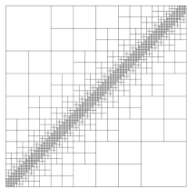
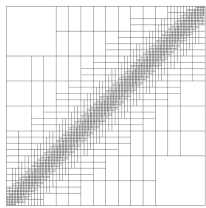
Refer to caption
(a) 1430 LR B-splines
Refer to caption
(b) 1894 LR B-splines
Refer to caption
(c) 2243 LR B-splines
Figure 10: Visual comparison between meshes of bidegree (2,2)22(2,2) obtained by performing 7 iterations of different mesh refinement strategies along the diagonal: (a) the structured LR-mesh, (b) the N2S2 LR-mesh, and (c) the LR-mesh proposed in [4].

In Figure 10(b) and Figure 11 one can see how the refinement in the N2S2 LR-meshes propagates from the region where the structured mesh refinement has been applied. In all the considered cases, the refinement does not heavily spread out. It is important to highlight, however, that the prolongation of the splits needed to recover the N2S-property is not unique. Indeed, when refining an LR B-spline to remove nestedness issues, the inserted split prolongations refine not only the considered LR B-spline but in general also other LR B-splines in the neighborhood. Then, some of the newly introduced neighboring LR B-splines might not need a one-directional tensor expansion anymore and the ordering used for removing nestedness has thus an effect on the resulting mesh.

One might consider to treat all the LR B-splines “in parallel”, i.e., first collect all the split extensions needed to remove nestedness in all the LR B-splines requiring a treatment and then insert all of them at the same time to refine the function basis. This could result in a more uniform propagation of the refinement out of the region where the structured mesh has been applied. On the other hand, by doing this, some split extensions could be unnecessary for recovering the N2S-property. Therefore, in general, also the number of LR B-splines on these meshes would be higher than the number obtained when treating one LR B-spline at a time. In the examples presented in this paper we do not remove nestedness “in parallel”. Hence, the resulting N2S2 LR-meshes depend on the order used when the one-directional tensor expansions are applied. On the other hand, the number of LR B-splines will be closer to the number of LR B-splines obtained when performing only the structured mesh refinement, i.e., closer to the “optimal” number of LR B-splines needed to reduce the error while preserving the local linear independence.
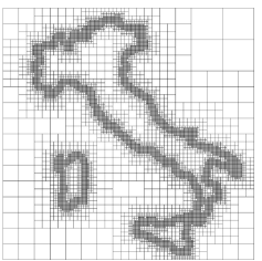
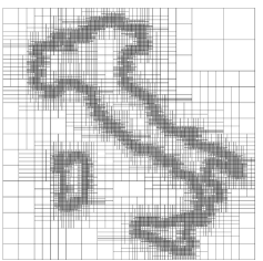
Refer to caption
(a) 10281 LR B-splines
Refer to caption
(b) 12438 LR B-splines
Refer to caption
(c) 13459 LR B-splines
Refer to caption
(d) 15993 LR B-splines
Refer to caption
(e) 8608 LR B-splines
Refer to caption
(f) 10841 LR B-splines
Figure 11: Meshes of bidegree (2,2)22(2,2) obtained by performing 8 iterations of mesh refinement on 3 different regions resulting in a structured LR-mesh (left column) and an N2S2 LR-mesh (right column).

We finally remark that one might also opt for full tensor expansions in the supports, instead of one-directional tensor expansions, to solve nestedness issues. The proof of Theorem 3.11 could be easily rephrased for the case of full tensor expansions. The key is that we only prolong splits provided by the structured mesh refinement performed at the beginning of the process. Therefore, if we do full tensor expansions, in the worst case scenario we would end up with a standard tensor mesh of size h=2(i+1)superscript2𝑖1h=2^{-(i+1)} to define the set i+1superscript𝑖1\mathcal{B}^{i+1}, instead of an LR-mesh tensorized in one direction. In such case, \mathcal{B} would still become empty in a finite number of loop iterations. However, we decided to do the expansion of the splits only in one direction at a time because it results in the least propagation.

4 Application I: Quasi-interpolation

A quasi-interpolation method is a procedure to compute the coefficients assigned to the basis elements of a prescribed function space, with the aim of approximating a given arbitrary function or data set. The resulting approximant is called a quasi-interpolant (QI). The computation of any of such coefficients may depend only on the data/function restricted to the corresponding basis element’s support (local method), and perhaps some neighboring other basis elements’ supports, or it can depend on the data/function in the entire domain (global method), as in the least-squares method. Given a function f𝑓f and an approximation space, whose basis is denoted by \mathcal{B}, we write a related QI in the form

𝔔f:=BλB(f)B,assign𝔔𝑓subscript𝐵subscript𝜆𝐵𝑓𝐵\mathfrak{Q}f:=\sum_{B\in\mathcal{B}}\lambda_{B}(f)B,

where λB(f)subscript𝜆𝐵𝑓\lambda_{B}(f) is the coefficient of the basis element B𝐵B\in\mathcal{B} computed by the selected method.

Definition 4.12.

A quasi-interpolation method such that 𝔔f=f𝔔𝑓𝑓\mathfrak{Q}f=f for all f𝑓f in a space V𝑉V is said to reproduce the space V𝑉V.

When using spline spaces of bidegree 𝒑𝒑\boldsymbol{p} as approximation spaces, a common requirement is that the polynomial space Π𝒑subscriptΠ𝒑\Pi_{\boldsymbol{p}} is reproduced by the quasi-interpolation method, in order to ensure good approximation properties. A general recipe for constructing local quasi-interpolation methods for tensor spline spaces, with the polynomial reproduction property, can be found in [16].

Recipe 4.13.

Let f𝑓f be a given function defined on the rectangle ΩΩ\Omega. Given a bidegree 𝐩𝐩\boldsymbol{p}, let ~~\widetilde{{\mathcal{M}}} be an open tensor mesh on ΩΩ\Omega, and let (~)~\mathcal{B}(\widetilde{{\mathcal{M}}}) be the set of tensor B-splines of bidegree 𝐩𝐩\boldsymbol{p} on ~~\widetilde{{\mathcal{M}}}. We compute the coefficient λB(f)subscript𝜆𝐵𝑓\lambda_{B}(f), for every B=B[𝐱,𝐲](~)𝐵𝐵𝐱𝐲~B=B[\boldsymbol{x},\boldsymbol{y}]\in\mathcal{B}(\widetilde{{\mathcal{M}}}), as follows.

  1. 1.

    Let U2𝑈superscript2U\subseteq{\mathbb{R}}^{2} be an open set that intersects the interior of suppBsupp𝐵\text{supp}\,B (for instance, U𝑈U can be a box-partition element of (𝒙,𝒚)𝒙𝒚{\mathcal{M}}(\boldsymbol{x},\boldsymbol{y})), and let (U)𝑈\mathcal{B}(U) be the subset of (~)~\mathcal{B}(\widetilde{{\mathcal{M}}}) consisting of all the tensor B-splines not identically zero on U𝑈U.

  2. 2.

    Choose a local polynomial approximation method 𝔓Usubscript𝔓𝑈\mathfrak{P}_{U} such that 𝔓Ug=gsubscript𝔓𝑈𝑔𝑔\mathfrak{P}_{U}g=g for all gΠ𝒑𝑔subscriptΠ𝒑g\in\Pi_{\boldsymbol{p}} defined on U𝑈U (typical choices are least-squares or interpolation methods). Letting g|Ug_{|U} be the restriction of g𝑔g to U𝑈U, we can write

    (𝔓Uf)|U=B~(U)bB~(f)B~|U,(\mathfrak{P}_{U}f)_{|U}=\sum_{\widetilde{B}\in\mathcal{B}(U)}b_{\widetilde{B}}(f)\widetilde{B}_{|U},

    for some coefficients bB~(f)subscript𝑏~𝐵𝑓b_{\widetilde{B}}(f) provided by the chosen local approximation method.

  3. 3.

    Since B(U)𝐵𝑈B\in\mathcal{B}(U), set λB(f):=bB(f)assignsubscript𝜆𝐵𝑓subscript𝑏𝐵𝑓\lambda_{B}(f):=b_{B}(f).

Then, define

𝔔f:=B(~)λB(f)B.assign𝔔𝑓subscript𝐵~subscript𝜆𝐵𝑓𝐵\mathfrak{Q}f:=\sum_{B\in\mathcal{B}(\widetilde{{\mathcal{M}}})}\lambda_{B}(f)B.

Inspired by the above recipe for tensor splines and similar to the local quasi-interpolation strategy developed for THB-splines in [25, 24], we can formulate a general recipe for constructing QIs in the space spanned by ()superscript\mathcal{B}^{\mathcal{LR}}({\mathcal{M}}) on a given open LR-mesh {\mathcal{M}} as follows: select for each LR B-spline B𝐵B in ()superscript\mathcal{B}^{\mathcal{LR}}({\mathcal{M}}) a local tensor space containing B𝐵B, and pick the coefficient corresponding to B𝐵B in the expression of any QI in such a tensor space. In particular, when the smallest local tensor space containing each basis function B𝐵B is considered, we arrive at the following recipe.

Recipe 4.14.

Let f𝑓f be a given function defined on the rectangle ΩΩ\Omega. Given a bidegree 𝐩𝐩\boldsymbol{p}, let {\mathcal{M}} be an open LR-mesh on ΩΩ\Omega, and let ()superscript\mathcal{B}^{\mathcal{LR}}({\mathcal{M}}) be the set of LR B-splines of bidegree 𝐩𝐩\boldsymbol{p} on {\mathcal{M}}. We compute the coefficient λB(f)subscript𝜆𝐵𝑓\lambda_{B}(f), for every B=B[𝐱,𝐲]()𝐵𝐵𝐱𝐲superscriptB=B[\boldsymbol{x},\boldsymbol{y}]\in\mathcal{B}^{\mathcal{LR}}({\mathcal{M}}), as follows.

  1. 1.

    Let ~Bsubscript~𝐵\widetilde{{\mathcal{M}}}_{B} be the open (tensor) mesh obtained by rising the boundary meshline multiplicities of B=(𝒙,𝒚)subscript𝐵𝒙𝒚{\mathcal{M}}_{B}={\mathcal{M}}(\boldsymbol{x},\boldsymbol{y}) to full multiplicity, and let (~B)subscript~𝐵\mathcal{B}(\widetilde{{\mathcal{M}}}_{B}) be the set of tensor B-splines defined on ~Bsubscript~𝐵\widetilde{{\mathcal{M}}}_{B}.

  2. 2.

    Consider a quasi-interpolation method in the space spanned by (~B)subscript~𝐵\mathcal{B}(\widetilde{{\mathcal{M}}}_{B}),

    𝔔Bf=B~(~B)bB~(f)B~,subscript𝔔𝐵𝑓subscript~𝐵subscript~𝐵subscript𝑏~𝐵𝑓~𝐵\mathfrak{Q}_{B}f=\sum_{\widetilde{B}\in\mathcal{B}(\widetilde{{\mathcal{M}}}_{B})}b_{\widetilde{B}}(f)\widetilde{B},

    reproducing all gΠ𝒑𝑔subscriptΠ𝒑g\in\Pi_{\boldsymbol{p}} (for instance, use Recipe 4.13).

  3. 3.

    Since B(~B)𝐵subscript~𝐵B\in\mathcal{B}(\widetilde{{\mathcal{M}}}_{B}), set λB(f):=bB(f)assignsubscript𝜆𝐵𝑓subscript𝑏𝐵𝑓\lambda_{B}(f):=b_{B}(f).

Then, define

𝔔f:=B()λB(f)B.assign𝔔𝑓subscript𝐵superscriptsubscript𝜆𝐵𝑓𝐵\mathfrak{Q}f:=\sum_{B\in\mathcal{B}^{\mathcal{LR}}({\mathcal{M}})}\lambda_{B}(f)B.

Since B(~B)𝐵subscript~𝐵B\in\mathcal{B}(\widetilde{{\mathcal{M}}}_{B}) for any B()𝐵superscriptB\in\mathcal{B}^{\mathcal{LR}}({\mathcal{M}}), the function 𝔔f𝔔𝑓\mathfrak{Q}f in Recipe 4.14 is well defined. Moreover, it will reproduce polynomials on the entire domain if the LR-mesh has the N2S-property as stated in the following proposition.

Proposition 4.15.

Given a bidegree 𝐩𝐩\boldsymbol{p}, let {\mathcal{M}} be an open LR-mesh and let ()superscript\mathcal{B}^{\mathcal{LR}}({\mathcal{M}}) be the set of LR B-splines of bidegree 𝐩𝐩\boldsymbol{p} on {\mathcal{M}}. Assume that {\mathcal{M}} has the N2S-property, then

𝔔g=g,gΠ𝒑,formulae-sequence𝔔𝑔𝑔for-all𝑔subscriptΠ𝒑\mathfrak{Q}g=g,\quad\forall g\in\Pi_{\boldsymbol{p}},

where the quasi-interpolation operator 𝔔𝔔\mathfrak{Q} is defined in Recipe 4.14.

Proof.

From [3, Theorem 4.6], if {\mathcal{M}} has the N2S-property, then for all gΠ𝒑𝑔subscriptΠ𝒑g\in\Pi_{\boldsymbol{p}} we have

g=B()gBB,gB,formulae-sequence𝑔subscript𝐵superscriptsubscript𝑔𝐵𝐵subscript𝑔𝐵g=\sum_{B\in\mathcal{B}^{\mathcal{LR}}({\mathcal{M}})}g_{B}B,\quad g_{B}\in{\mathbb{R}},

where for all B()𝐵superscriptB\in\mathcal{B}^{\mathcal{LR}}({\mathcal{M}}), the coefficient gBsubscript𝑔𝐵g_{B} only depends on g𝑔g and on the knots defining the LR B-spline B𝐵B. Therefore, gBsubscript𝑔𝐵g_{B} remains the same if we represent g𝑔g in any set of tensor B-splines containing B𝐵B. Since, according to Recipe 4.14, any 𝔔Bsubscript𝔔𝐵\mathfrak{Q}_{B} reproduces all polynomials in Π𝒑subscriptΠ𝒑\Pi_{\boldsymbol{p}} we have

gB=λB(g),B(),gΠ𝒑,formulae-sequencesubscript𝑔𝐵subscript𝜆𝐵𝑔formulae-sequencefor-all𝐵superscript𝑔subscriptΠ𝒑g_{B}=\lambda_{B}(g),\quad\forall B\in\mathcal{B}^{\mathcal{LR}}({\mathcal{M}}),\quad g\in\Pi_{\boldsymbol{p}},

which completes the proof. ∎

{floatrow}\ffigboxRefer to caption
Figure 12: Transcendent function in [1,1]2superscript112[-1,1]^{2}.
\capbtabbox
# basis functions
levels Tensor mesh N2S2 LR-mesh max error
1 36 36 5.686e-01
2 100 86 4.645e-01
3 324 161 2.575e-01
4 1156 254 1.472e-01
5 4356 363 5.955e-02
6 16900 450 2.156e-02
7 66564 537 1.415e-02
Figure 13: B-spline set cardinalities of bidegree (2,2)22(2,2) for different levels of maximal resolution.

We have tested the quasi-interpolation strategy described in Recipe 4.14 on N2S2 LR-meshes to approximate polynomials and transcendent functions. Given an N2S2 LR-mesh {\mathcal{M}}, this recipe requires the construction of a QI based on (~B)subscript~𝐵\mathcal{B}(\widetilde{{\mathcal{M}}}_{B}) for each of the LR B-splines B()𝐵superscriptB\in\mathcal{B}^{\mathcal{LR}}({\mathcal{M}}) of bidegree 𝒑=(p1,p2)𝒑subscript𝑝1subscript𝑝2\boldsymbol{p}=(p_{1},p_{2}). Following Recipe 4.13, we have used interpolation as local approximation method in the computation of these QIs. More precisely, we have selected a unisolvent set of (p1+1)(p2+1)subscript𝑝11subscript𝑝21(p_{1}+1)(p_{2}+1) interpolation points, organized in a tensor grid over a single box-partition element of ~Bsubscript~𝐵\widetilde{{\mathcal{M}}}_{B}, and then we have set a linear system by evaluating f𝑓f and the tensor B-splines in (~B)subscript~𝐵\mathcal{B}(\widetilde{{\mathcal{M}}}_{B}) at these points. This guarantees polynomial reproduction (actually spline reproduction) of the quasi-interpolation method in the spaces (~B)subscript~𝐵\mathcal{B}(\widetilde{{\mathcal{M}}}_{B}), for B𝐵B varying in ()superscript\mathcal{B}^{\mathcal{LR}}({\mathcal{M}}). Therefore, also the resulting quasi-interpolation method on ()superscript\mathcal{B}^{\mathcal{LR}}({\mathcal{M}}) has the polynomial reproduction property thanks to Proposition 4.15. Indeed, in all the tests with polynomial functions of bidegree at most 𝒑𝒑\boldsymbol{p}, the maximum error was in the order of the machine precision, regardless of the number of iterations performed to construct the N2S2 LR-mesh. The maximum error was computed on a uniform 150 ×\times 150 grid.

As test with a transcendent function, we have considered

f(x,y)=23e(10x3)2+(10y3)2+23e(10x+3)2+(10y+3)2+23e(10x)2+(10y)2,𝑓𝑥𝑦23superscript𝑒superscript10𝑥32superscript10𝑦3223superscript𝑒superscript10𝑥32superscript10𝑦3223superscript𝑒superscript10𝑥2superscript10𝑦2f(x,y)=\frac{2}{3}e^{-\sqrt{(10x-3)^{2}+(10y-3)^{2}}}+\frac{2}{3}e^{-\sqrt{(10x+3)^{2}+(10y+3)^{2}}}+\frac{2}{3}e^{-\sqrt{(10x)^{2}+(10y)^{2}}},

which is characterized by three steep peaks on the square [1,1]2superscript112[-1,1]^{2} located at (0.3,0.3)0.30.3(-0.3,-0.3), (0,0)00(0,0) and (0.3,0.3)0.30.3(0.3,0.3); see Figure 13. This function has also been used in [25] to investigate the approximation power of a similar quasi-interpolation method developed for THB-splines. In Table 13, we compare the number of basis functions of bidegree (2,2)22(2,2) when considering global tensor meshes and local N2S2 LR-meshes for different levels of maximal resolution (for level \ell, the smallest box-partition elements on the mesh have length 2superscript22^{-\ell}). The N2S2 LR-mesh is obtained by refining the LR B-splines whose supports contain one of the three points where a peak occurs via structured mesh refinement and then by recovering the N2S-property via one-directional tensor expansions. For a given maximal resolution level, the optimal maximum error, i.e., the maximum error when using the global tensor mesh, is preserved by the N2S2 LR-mesh. However, the number of B-splines is significantly different and the discrepancy exponentially grows with the maximal resolution level.

5 Application II: Isogeometric analysis

Isogeometric analysis (IgA), introduced in [14], is a technique to perform numerical simulations on complex geometries. The numerical solution is represented by means of the same functions used for the domain modeling. Nowadays, complex geometries are expressed in terms of computed aided design (CAD) technologies, such as B-splines, non-uniform rational B-splines (NURBS) and their generalizations to address adaptive refinements.

In this section, we adopt the IgA approach, using our LR refinement strategy, to approximate the solution of the Poisson problem on Ω=[0,1]2Ωsuperscript012\Omega=[0,1]^{2},

{Δu=f,in Ω̊,u=uD,on Ω,casesΔ𝑢𝑓in ̊Ω𝑢subscript𝑢𝐷on Ω\left\{\begin{array}[]{rl}-\Delta u=f,&\mbox{in }\mathring{\Omega},\\ u=u_{D},&\mbox{on }\partial\Omega,\end{array}\right. (2)

whose exact solution is

u(x,y)=arctan(100((x1.25)2+(y+0.25)2π3));𝑢𝑥𝑦100superscript𝑥1.252superscript𝑦0.252𝜋3u(x,y)=\arctan\left(100\left(\sqrt{(x-1.25)^{2}+(y+0.25)^{2}}-\frac{\pi}{3}\right)\right);

see Figure 14. This example is a good benchmark for numerical schemes, as the sharp interior layer of the exact solution highlights the approximation quality, and it has been used extensively in the literature; see, e.g., [19, 15, 6].
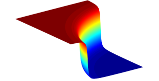
Refer to caption
Figure 14: Exact solution of the Poisson problem (2).

In the context of Galerkin discretizations, two properties are desirable:

  • 1.

    (local) linear independence of the space generators,

  • 2.

    refinement adaptivity.

The linear independence of the functions used as building blocks of the numerical solution avoids the numerical complexity posed by the singularity of the matrices associated to the problem discretization. The refinement adaptivity is desired for balancing accuracy and computational cost as it allows for a higher precision, only there where it is needed to reproduce fast variations of the exact solution. LR B-splines on N2S2 LR-meshes are suitable candidates as both the (local) linear independence of the space generators and the adaptivity of the refinement are guaranteed.
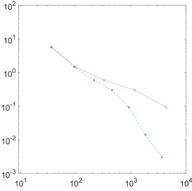
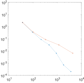
Refer to caption
(a)
Refer to caption
(b)
Figure 15: Decay of the error in (a) the Lsuperscript𝐿L^{\infty}-norm and (b) the L2superscript𝐿2L^{2}-norm, when approximating the solution of problem (2) with B-splines of bidegree (2,2)22(2,2) on tensor meshes (solid line) and N2S2 LR-meshes (dashed line) for different levels of maximal resolution.

In Figure 15 we compare the Lsuperscript𝐿L^{\infty}-norm and the L2superscript𝐿2L^{2}-norm of the error (Figures 15(a) and 15(b) respectively), using bidegree (2,2)22(2,2) with global tensor meshes and local N2S2 LR-meshes for different levels of maximal resolution to approximate the solution of the Poisson problem (2). The N2S2 LR-mesh is computed by first applying the structured mesh to the LR B-splines whose supports intersect the curve where the sharp interior layer in the exact solution occurs, and then by performing one-directional tensor expansions to recover the N2S-property. The error norms, which are computed discretely on a uniform grid of 1000×1000100010001000\times 1000 points, are plotted in log-log scale with respect to the number of LR B-splines on the mesh. The solid line with circular markers shows the decay when using global tensor meshes, whereas the dashed line with star markers shows the decay for the N2S2 LR-meshes. In the figures, the first marker corresponds to the 4×4444\times 4 tensor mesh, for maximal resolution level =22\ell=2, and it is the maximal level for which the LR B-spline and standard tensor B-spline sets coincide. When considering a comparable number of functions, the N2S2 LR-mesh leads to a significant reduction of both the Lsuperscript𝐿L^{\infty}-norm and the L2superscript𝐿2L^{2}-norm of the error with respect to the tensor mesh, thanks to the adaptivity of the refinement.

6 Conclusion

LR B-splines are one of the most elegant extensions of univariate B-splines on local tensor structures that allow local refinement. They possess almost all the properties of classical B-splines, but they are not always linearly independent. Recently, a characterization of LR-meshes ensuring local linear independence of the corresponding LR B-splines has been presented in the literature. However, a practical adaptive refinement strategy for LR-meshes that maintain such a property was missing. In this paper, we have filled this gap by describing an adaptive refinement strategy that generates LR-meshes where the corresponding LR B-splines are locally linearly independent. Subsequently, we have exploited the local linear independence of the LR B-splines to construct efficient quasi-interpolation schemes and to solve elliptic problems using the isogeometric Galerkin method.

Acknowledgements

We are very grateful to Tor Dokken (SINTEF, Oslo) and Kjetil André Johannessen (SINTEF, Trondheim) for sharing with us the example in Figure 8 that shows that the standard structured mesh refinement may produce linearly dependent sets of LR B-splines.

Appendix A Nested LR B-splines

The purpose of this appendix is to show the equivalence of the definition of nestedness used in this paper (Definition 2.6) and the original definition provided in [3, Definition 2.4] for LR B-splines. The latter definition is formulated in terms of repeated knot insertion and, in view of [3, Proposition 2.5], it is equivalent to the following definition.

Definition A.16.

Let B[𝐱1,𝐲1]𝐵superscript𝐱1superscript𝐲1B[\boldsymbol{x}^{1},\boldsymbol{y}^{1}] and B[𝐱2,𝐲2]𝐵superscript𝐱2superscript𝐲2B[\boldsymbol{x}^{2},\boldsymbol{y}^{2}] be two different tensor B-splines. Let μ𝐱k(z)subscript𝜇superscript𝐱𝑘𝑧\mu_{\boldsymbol{x}^{k}}(z) and μ𝐲k(z)subscript𝜇superscript𝐲𝑘𝑧\mu_{\boldsymbol{y}^{k}}(z), for k=1,2𝑘12k=1,2, denote the number of times z𝑧z\in{\mathbb{R}} occurs in the vectors 𝐱ksuperscript𝐱𝑘\boldsymbol{x}^{k} and 𝐲ksuperscript𝐲𝑘\boldsymbol{y}^{k}, respectively. Then, we say that B[𝐱2,𝐲2]𝐵superscript𝐱2superscript𝐲2B[\boldsymbol{x}^{2},\boldsymbol{y}^{2}] is nested in B[𝐱1,𝐲1]𝐵superscript𝐱1superscript𝐲1B[\boldsymbol{x}^{1},\boldsymbol{y}^{1}], and we write B[𝐱2,𝐲2]B[𝐱1,𝐲1]precedes-or-equals𝐵superscript𝐱2superscript𝐲2𝐵superscript𝐱1superscript𝐲1B[\boldsymbol{x}^{2},\boldsymbol{y}^{2}]\preceq B[\boldsymbol{x}^{1},\boldsymbol{y}^{1}], if

  1. 1.

    {μ𝒙2(z)μ𝒙1(z),z]x12,xp1+22[,μ𝒚2(z)μ𝒚1(z),z]y12,yp2+22[,\left\{\begin{array}[]{ll}\mu_{\boldsymbol{x}^{2}}(z)\geq\mu_{\boldsymbol{x}^{1}}(z),&\forall\,z\in\;]x_{1}^{2},x_{p_{1}+2}^{2}[,\\[5.69046pt] \mu_{\boldsymbol{y}^{2}}(z)\geq\mu_{\boldsymbol{y}^{1}}(z),&\forall\,z\in\;]y_{1}^{2},y_{p_{2}+2}^{2}[,\\[2.84544pt] \end{array}\right.

  2. 2.

    {μ𝒙2(z)μ𝒙1(z),z]x11,xp1+21[,μ𝒚2(z)μ𝒚1(z),z]y11,yp2+21[.\left\{\begin{array}[]{ll}\mu_{\boldsymbol{x}^{2}}(z)\leq\mu_{\boldsymbol{x}^{1}}(z),&\forall\,z\notin\;]x_{1}^{1},x_{p_{1}+2}^{1}[,\\[5.69046pt] \mu_{\boldsymbol{y}^{2}}(z)\leq\mu_{\boldsymbol{y}^{1}}(z),&\forall\,z\notin\;]y_{1}^{1},y_{p_{2}+2}^{1}[.\\[2.84544pt] \end{array}\right.

We now prove the equivalence of the two definitions for LR B-splines.

Proposition A.17.

Given a mesh {\mathcal{M}}, let B[𝐱1,𝐲1]𝐵superscript𝐱1superscript𝐲1B[\boldsymbol{x}^{1},\boldsymbol{y}^{1}] and B[𝐱2,𝐲2]𝐵superscript𝐱2superscript𝐲2B[\boldsymbol{x}^{2},\boldsymbol{y}^{2}] be two different LR B-splines defined on {\mathcal{M}}. For B[𝐱1,𝐲1]𝐵superscript𝐱1superscript𝐲1B[\boldsymbol{x}^{1},\boldsymbol{y}^{1}] and B[𝐱2,𝐲2]𝐵superscript𝐱2superscript𝐲2B[\boldsymbol{x}^{2},\boldsymbol{y}^{2}], Definition 2.6 is equivalent to Definition A.16.

Proof.

Let B1:=B[𝒙1,𝒚1]assignsuperscript𝐵1𝐵superscript𝒙1superscript𝒚1B^{1}:=B[\boldsymbol{x}^{1},\boldsymbol{y}^{1}] and B2:=B[𝒙2,𝒚2]assignsuperscript𝐵2𝐵superscript𝒙2superscript𝒚2B^{2}:=B[\boldsymbol{x}^{2},\boldsymbol{y}^{2}] be two LR B-splines defined on the mesh {\mathcal{M}}. Assuming that they satisfy the conditions in Definition A.16, we prove that they also satisfy the conditions in Definition 2.6. Let us first show that suppB2suppB1suppsuperscript𝐵2suppsuperscript𝐵1\text{supp}\,B^{2}\subseteq\text{supp}\,B^{1}. This means that [x12,xp1+22][x11,xp1+21]superscriptsubscript𝑥12superscriptsubscript𝑥subscript𝑝122superscriptsubscript𝑥11superscriptsubscript𝑥subscript𝑝121[x_{1}^{2},x_{p_{1}+2}^{2}]\subseteq[x_{1}^{1},x_{p_{1}+2}^{1}] and [y12,yp2+22][y11,yp2+21]superscriptsubscript𝑦12superscriptsubscript𝑦subscript𝑝222superscriptsubscript𝑦11superscriptsubscript𝑦subscript𝑝221[y_{1}^{2},y_{p_{2}+2}^{2}]\subseteq[y_{1}^{1},y_{p_{2}+2}^{1}]. Suppose x12<x11superscriptsubscript𝑥12superscriptsubscript𝑥11x_{1}^{2}<x_{1}^{1}. Then, μ𝒙1(x12)=0subscript𝜇superscript𝒙1superscriptsubscript𝑥120\mu_{\boldsymbol{x}^{1}}(x_{1}^{2})=0 and μ𝒙2(x12)>0subscript𝜇superscript𝒙2superscriptsubscript𝑥120\mu_{\boldsymbol{x}^{2}}(x_{1}^{2})>0, but this contradicts item 2 in Definition A.16, and hence x12x11superscriptsubscript𝑥12superscriptsubscript𝑥11x_{1}^{2}\geq x_{1}^{1}. The other inequalities can be proved in a similar way to have the interval inclusions. Let now γsuppB1suppB2𝛾suppsuperscript𝐵1suppsuperscript𝐵2\gamma\subseteq\partial\text{supp}\,B^{1}\cap\partial\text{supp}\,B^{2}. Assume without loss of generality that γ𝛾\gamma is a 111-meshline. Then, γ𝛾\gamma is a (1,z)1𝑧(1,z)-meshlines for some z{x11,xp1+21}𝑧superscriptsubscript𝑥11superscriptsubscript𝑥subscript𝑝121z\in\{x_{1}^{1},x_{p_{1}+2}^{1}\}. For any choice of such z𝑧z, we have μ𝒙2(z)μ𝒙1(z)subscript𝜇superscript𝒙2𝑧subscript𝜇superscript𝒙1𝑧\mu_{\boldsymbol{x}^{2}}(z)\leq\mu_{\boldsymbol{x}^{1}}(z), by item 2 of Definition A.16, and, by the definition of multiplicity of γ𝛾\gamma in (𝒙1,𝒚1)superscript𝒙1superscript𝒚1{\mathcal{M}}(\boldsymbol{x}^{1},\boldsymbol{y}^{1}) and (𝒙2,𝒚2)superscript𝒙2superscript𝒚2{\mathcal{M}}(\boldsymbol{x}^{2},\boldsymbol{y}^{2}), this implies that μ(γ)𝜇𝛾\mu(\gamma) is higher (or equal) in (𝒙1,𝒚1)superscript𝒙1superscript𝒚1{\mathcal{M}}(\boldsymbol{x}^{1},\boldsymbol{y}^{1}) than in (𝒙2,𝒚2)superscript𝒙2superscript𝒚2{\mathcal{M}}(\boldsymbol{x}^{2},\boldsymbol{y}^{2}). Therefore, both the conditions in Definition 2.6 are satisfied if those in Definition A.16 are satisfied.

Let us now show the converse. Assuming that the conditions in Definition 2.6 are fulfilled, we prove that the conditions in Definition A.16 are satisfied as well. Let z]x12,xp1+22[z\in\;]x_{1}^{2},x_{p_{1}+2}^{2}[. Since suppB2suppB1suppsuperscript𝐵2suppsuperscript𝐵1\text{supp}\,B^{2}\subseteq\text{supp}\,B^{1}, we have ]x12,xp1+22[]x11,xp1+21[]x_{1}^{2},x_{p_{1}+2}^{2}[\;\subseteq\;]x_{1}^{1},x_{p_{1}+2}^{1}[. If z𝒙1𝑧superscript𝒙1z\notin\boldsymbol{x}^{1}, then μ𝒙1(z)=0subscript𝜇superscript𝒙1𝑧0\mu_{\boldsymbol{x}^{1}}(z)=0 and therefore μ𝒙2(z)μ𝒙1(z)subscript𝜇superscript𝒙2𝑧subscript𝜇superscript𝒙1𝑧\mu_{\boldsymbol{x}^{2}}(z)\geq\mu_{\boldsymbol{x}^{1}}(z) for any value of μ𝒙2(z)subscript𝜇superscript𝒙2𝑧\mu_{\boldsymbol{x}^{2}}(z). If z𝒙1𝑧superscript𝒙1z\in\boldsymbol{x}^{1}, then it must be also in 𝒙2superscript𝒙2\boldsymbol{x}^{2}, otherwise the (1,z)1𝑧(1,z)-split {z}×[y11,yp2+21]𝑧superscriptsubscript𝑦11superscriptsubscript𝑦subscript𝑝221\{z\}\times[y_{1}^{1},y_{p_{2}+2}^{1}] would traverse B2superscript𝐵2B^{2}, which would not have minimal support. For the same reason, it must also hold that μ𝒙2(z)=μ𝒙1(z)subscript𝜇superscript𝒙2𝑧subscript𝜇superscript𝒙1𝑧\mu_{\boldsymbol{x}^{2}}(z)=\mu_{\boldsymbol{x}^{1}}(z). This proves item 1 of Definition A.16. Assume now z[x11,xp1+21]𝑧superscriptsubscript𝑥11superscriptsubscript𝑥subscript𝑝121z\notin[x_{1}^{1},x_{p_{1}+2}^{1}]. Since suppB2suppB1suppsuperscript𝐵2suppsuperscript𝐵1\text{supp}\,B^{2}\subseteq\text{supp}\,B^{1}, we have x11x12superscriptsubscript𝑥11superscriptsubscript𝑥12x_{1}^{1}\leq x_{1}^{2} and xp1+22xp1+21superscriptsubscript𝑥subscript𝑝122superscriptsubscript𝑥subscript𝑝121x_{p_{1}+2}^{2}\leq x_{p_{1}+2}^{1}. Therefore, μ𝒙1(z)=μ𝒙2(z)=0subscript𝜇superscript𝒙1𝑧subscript𝜇superscript𝒙2𝑧0\mu_{\boldsymbol{x}^{1}}(z)=\mu_{\boldsymbol{x}^{2}}(z)=0. If z{x11,xp1+21}𝑧superscriptsubscript𝑥11superscriptsubscript𝑥subscript𝑝121z\in\{x_{1}^{1},x_{p_{1}+2}^{1}\} but z𝒙2𝑧superscript𝒙2z\notin\boldsymbol{x}^{2}, then trivially μ𝒙2(z)μ𝒙1(z)subscript𝜇superscript𝒙2𝑧subscript𝜇superscript𝒙1𝑧\mu_{\boldsymbol{x}^{2}}(z)\leq\mu_{\boldsymbol{x}^{1}}(z). If z𝒙2𝑧superscript𝒙2z\in\boldsymbol{x}^{2}, then z𝑧z corresponds to (1,z)1𝑧(1,z)-meshlines in suppB1suppB2suppsuperscript𝐵1suppsuperscript𝐵2\partial\text{supp}\,B^{1}\cap\partial\text{supp}\,B^{2}. By assumption, these meshlines have a higher (or equal) multiplicity in (𝒙1,𝒚1)superscript𝒙1superscript𝒚1{\mathcal{M}}(\boldsymbol{x}^{1},\boldsymbol{y}^{1}) than in (𝒙2,𝒚2)superscript𝒙2superscript𝒚2{\mathcal{M}}(\boldsymbol{x}^{2},\boldsymbol{y}^{2}), which means μ𝒙2(z)μ𝒙1(z)subscript𝜇superscript𝒙2𝑧subscript𝜇superscript𝒙1𝑧\mu_{\boldsymbol{x}^{2}}(z)\leq\mu_{\boldsymbol{x}^{1}}(z). The same line of arguments also applies to the knots in the second direction. This proves item 2 of Definition A.16. ∎

References

  • [1] L. Beirão da Veiga, A. Buffa, G. Sangalli, and R. Vázquez, Mathematical analysis of variational isogeometric methods, Acta Numerica 23 (2014), 157–287.
  • [2] C. de Boor, A practical guide to splines, revised ed., Springer-Verlag New York, 2001.
  • [3] A. Bressan, Some properties of LR-splines, Computer Aided Geometric Design 30 (2013), no. 8, 778–794.
  • [4] A. Bressan and B. Jüttler, A hierarchical construction of LR meshes in 2D, Computer Aided Geometric Design 37 (2015), 9–24.
  • [5] A. Buffa, D. Cho, and G. Sangalli, Linear independence of the T-spline blending functions associated with some particular T-meshes, Computer Methods in Applied Mechanics and Engineering 199 (2010), no. 23-24, 1437–1445.
  • [6] J. Cao, Z. Chen, X. Wei, and Y. J. Zhang, A finite element framework based on bivariate simplex splines on triangle configurations, Computer Methods in Applied Mechanics and Engineering 357 (2019), 112598.
  • [7] E. Cohen, R. F. Riesenfeld, and G. Elber, Geometric modeling with splines: An introduction, A K Peters, Wellesley, 2001.
  • [8] J. A. Cottrell, T. J. R. Hughes, and Y. Bazilevs, Isogeometric analysis: Toward integration of CAD and FEA, John Wiley & Sons, Chichester, 2009.
  • [9] J. Deng, F. Chen, X. Li, C. Hu, W. Tong, Z. Yang, and Y. Feng, Polynomial splines over hierarchical T-meshes, Graphical models 70 (2008), no. 4, 76–86.
  • [10] T. Dokken, T. Lyche, and K. F. Pettersen, Polynomial splines over locally refined box-partitions, Computer Aided Geometric Design 30 (2013), no. 3, 331–356.
  • [11] N. Engleitner and B. Jüttler, Patchwork B-spline refinement, Computer-Aided Design 90 (2017), 168–179.
  • [12] D. R. Forsey and R. H. Bartels, Hierarchical B-spline refinement, ACM Siggraph Computer Graphics 22 (1988), no. 4, 205–212.
  • [13] C. Giannelli, B. Jüttler, and H. Speleers, THB-splines: The truncated basis for hierarchical splines, Computer Aided Geometric Design 29 (2012), no. 7, 485–498.
  • [14] T. J. R. Hughes, J. A. Cottrell, and Y. Bazilevs, Isogeometric analysis: CAD, finite elements, NURBS, exact geometry and mesh refinement, Computer Methods in Applied Mechanics and Engineering 194 (2005), no. 39–41, 4135–4195.
  • [15] K. A. Johannessen, T. Kvamsdal, and T. Dokken, Isogeometric analysis using LR B-splines, Computer Methods in Applied Mechanics and Engineering 269 (2014), 471–514.
  • [16] B. G. Lee, T. Lyche, and K. Mørken, Some examples of quasi-interpolants constructed from local spline projectors, Mathematical Methods in CAGD: Oslo 2000 (T. Lyche and L. L. Schumaker, eds.), Vanderbilt University Press, Nashville, 2001, pp. 243–252.
  • [17] T. Lyche, C. Manni, and H. Speleers, Foundations of spline theory: B-splines, spline approximation, and hierarchical refinement, Splines and PDEs: From Approximation Theory to Numerical Linear Algebra (T. Lyche et al., eds.), Lecture Notes in Mathematics, vol. 2219, Springer International Publishing AG, 2018, pp. 1–76.
  • [18] C. Manni and H. Speleers, Standard and non-standard CAGD tools for isogeometric analysis: A tutorial, IsoGeometric Analysis: A New Paradigm in the Numerical Approximation of PDEs (A. Buffa and G. Sangalli, eds.), Lecture Notes in Mathematics, vol. 2161, Springer International Publishing AG, 2016, pp. 1–69.
  • [19] W. F. Mitchell and M. A. McClain, A survey of hp𝑝hp-adaptive strategies for elliptic partial differential equations, Recent Advances in Computational and Applied Mathematics (T. E. Simos, ed.), Springer Dordrecht, 2011, pp. 227–258.
  • [20] F. Patrizi and T. Dokken, Linear dependence of bivariate Minimal Support and Locally Refined B-splines over LR-meshes, Computer Aided Geometric Design (in press).
  • [21] L. Piegl and W. Tiller, The NURBS book, second ed., Springer-Verlag Berlin, 1997.
  • [22] L. L. Schumaker, Spline functions: Basic theory, third ed., Cambridge University Press, 2007.
  • [23] T. W. Sederberg, J. Zheng, A. Bakenov, and A. Nasri, T-splines and T-NURCCs, ACM Transactions on Graphics 22 (2003), no. 3, 477–484.
  • [24] H. Speleers, Hierarchical spline spaces: Quasi-interpolants and local approximation estimates, Advances in Computational Mathematics 43 (2017), no. 2, 235–255.
  • [25] H. Speleers and C. Manni, Effortless quasi-interpolation in hierarchical spaces, Numerische Mathematik 132 (2016), no. 1, 155–184.