A second-order exponential time differencing scheme for non-linear reaction-diffusion systems with dimensional splitting

E.O. Asante-Asamani nasmano@gmail.com Hunter College, City University of New York, New York City, NY 10065, USA A. Kleefeld a.kleefeld@fz-juelich.de Jรผlich Supercomputing Centre, Forschungszentrum Jรผlich GmbH, 52425 Jรผlich, Germany B.A. Wade bruce.wade@louisiana.edu Department of Mathematics, University of Louisiana at Lafayette, Lafayette, LA 70504-3568, USA
Abstract

A second-order L๐ฟL-stable exponential time-differencing (ETD) method is developed by combining an ETD scheme with approximating the matrix exponentials by rational functions having real distinct poles (RDP), together with a dimensional splitting integrating factor technique. A variety of non-linear reaction-diffusion equations in two and three dimensions with either Dirichlet, Neumann, or periodic boundary conditions are solved with this scheme and shown to outperform a variety of other second-order implicit-explicit schemes. An additional performance boost is gained through further use of basic parallelization techniques.

keywords:
Exponential time differencing , real distinct pole , dimensional splitting , reaction-diffusion systems , matrix exponential
MSC:
65M12 , 65M15 , 65M20 , 65F60
โ€ โ€ journal: arXiv

1 Introduction

Many applications, for example in biology [Murray2002, Murray2003, Mueller2015], pattern formation [Kondo2010], or medicine [Holmes21994, Sherrat1990] can be modelled with a system of s๐‘ s time-dependent non-linear reaction-diffusion equations in d๐‘‘d dimensions given by

โˆ‚๐ฎโˆ‚t=๐ƒโ€‹ฮ”โ€‹๐ฎ+๐…โ€‹(๐ฎ),๐ฑโˆˆฮฉโŠ‚โ„d,tโˆˆ(0,T)formulae-sequenceformulae-sequence๐ฎ๐‘ก๐ƒฮ”๐ฎ๐…๐ฎ๐ฑฮฉsuperscriptโ„๐‘‘๐‘ก0๐‘‡\displaystyle\frac{\partial\mathbf{u}}{\partial t}=\mathbf{D}\Delta\mathbf{u}+\mathbf{F}(\mathbf{u})\,,\qquad\mathbf{x}\in\Omega\subset\mathbb{R}^{d}\,,\quad t\in(0,T) (1)

with appropriate initial and boundary condition for the domain ฮฉฮฉ\Omega and the time interval (0,T)0๐‘‡(0,T). The numerical computation of such systems in two or three dimensions is challenging due to its high dimensionality, coupling, stiffness of the reaction and diffusion terms, and since the function ๐…๐…\mathbf{F} may be non-linear. Additionally, spurious oscillations in the approximate solution might occur if the initial data are non-smooth or are incompatible with the boundary data.

Many algorithms have been proposed to solve such systems after discretization in space. For example, linearly implicit methods [Akrivis1999, Vigo2007, Wade2001], semi-implicit methods [Chen1998], projection methods [Gear2003], stabilized explicit Runge-Kutta methods such as ROCK2 and ROCK4 [rock2, rock4], PIROCK [abdullepirock], SERK, SERK2V2, and SERK2V3 [serk2, serkv2, multi, serk2v3], its extrapolated variants [eserk4, eserk5, eserk6], explicit Runge-Kutta-Chebyshev (RKC) [rkc], implicit-explicit Runge-Kutta-Chebyshev (IRKC) [irkc] (one of many implicit-explicit methods (IMEX) [Hundsdorfer, ruuth]), factorized Runge-Kutta-Chebyshev (FRKC) or Runge-Kutta with Gegenbauer polynomials [Sul15, Sul19], integration factor methods [wang, Zhao] in combination with Krylov subspace methods [chen2011, donglu], and exponential propagation iterative methods of Runge-Kutta type (EPIRK) [tokman] and its variants such as IMEXP [luan], to mention a few.

One important family to solve the problem at hand is exponential time differencing (ETD), which uses the Duhamel principle and solves the resulting initial value problem by approximating the integral appropriately [Wade2009, Wade2012]. A class of ETD schemes based on Runge-Kutta methods has been introduced by Cox and Matthews [Cox2002]. Since then, many researchers have considered this scheme (see for example [Du2005, Hoch12005, hoch2005, minchev, Wade2009, kassamtrefethen]). However, the challenge of how to effectively approximate the matrix exponentials remains. Kleefeld, Khaliq, and Wade [Kleefeld2012, etdoption] considered an ETD Crank-Nicolson (ETD-CN) scheme; that is, the matrix exponential has been approximated through a second-order Padรฉ-(1,1)11(1,1) approximation. Their fully discrete scheme is of second-order and highly efficient, but it is not L๐ฟL-stable. Other schemes use Krylov subspace methods to approximate the matrix exponential [bhatt2018] or use higher order Padรฉ approximations [vigo2007a].

To speed up computations and to decrease memory demand, various dimensional splitting techniques such as, Strang simple and Strang symmetric splitting, as well as an integrating factor method have been considered by Asante-Asamani and Wade [asante2] for a variety of examples with Dirichlet and Neumann boundary conditions in two dimensions as a competitive alternative to the locally one-dimensional splitting of Bhatt and Khaliq [bhatt]. It has been observed empirically that the integrating factor approach outperforms other splitting techniques.

An extension of the work for ETD-CN with Padรฉ-(1,1)11(1,1) is given by Yousuf, Khaliq, and Kleefeld [Yousuf2012] using a Padรฉ-(0,2)02(0,2) approximation of the matrix exponential leading to a second-order L๐ฟL-stable scheme. However, one has to use complex arithmetic in the implementation due to the two complex-valued poles in the Padรฉ approximation. To avoid this, one can use a rational (non-Padรฉ) approximation of second-order with real distinct poles (see [Khaliq1994]), which has recently been applied by Asante-Asamani, Khaliq and Wade [asante] to the second-order ETD scheme, named hereafter ETD-RDP. It is shown that ETD-RDP is a competitive alternative to BDF2 [Vigo2007] and ETD-Padรฉ-(0,2)02(0,2) for a variety of examples with Dirichlet and Neumann boundary conditions in two dimensions. Further, it has been remarked by the authors that the ETD-RDP algorithm is easily parallelizable.

Contribution

In this work, we apply a splitting technique using an integrating factor (IF) approach to the second-order L๐ฟL-stable ETD-RDP scheme, lifting the derivation from two dimensions to d๐‘‘d dimensions, which we call ETD-RDP-IF. We show that besides Dirichlet and Neumann boundary conditions, also the periodic boundary condition case can be handled. Further, the algorithm can deal with non-smooth boundary conditions as well as with mismatching boundary conditions. Additionally, we explain how to solve the sparse linear systems in higher dimensions efficiently using an extension of the Thomas algorithm for Dirichlet and Neumann boundary conditions and using the Fourier transformation for periodic boundary conditions. Further, we describe how to implement a parallelization strategy in Fortran, and show that we developed a second-order L๐ฟL-stable method that is able to outperform other second-order IMEX schemes as well as ETD-RDP.

Organization of the paper

In Section 2, the mathematical model of a system consisting of s๐‘ s non-linear reaction-diffusion equations is detailed. Section 3 illustrates how this system is discretized in d๐‘‘d-dimensional space. The dimensional splitting using the integrating factor approach is given in Section 4. The discretization with respect to time using exponential time differencing is described in Section 5. In Section 6, we develop the approximation of the matrix exponential. The implementation and parallelization of the fully discrete ETD-RDP-IF scheme is given in Section 7. Extensive numerical results in two and three dimensions with Dirichlet, Neumann, and periodic boundary conditions are given in Section 8, which show the second-order accuracy and the efficiency of the new ETD-RDP-IF scheme. A short summary and a conclusion together with an outlook for possible future research is given in Section 9.

2 Time-dependent non-linear reaction-diffusion equation

The mathematical model of a system of s๐‘ s time-dependent non-linear reaction-diffusion equations in d๐‘‘d dimensions is given as

โˆ‚๐ฎโˆ‚t=๐ƒโ€‹ฮ”โ€‹๐ฎ+๐…โ€‹(๐ฎ),๐ฑโˆˆฮฉโŠ‚โ„d,tโˆˆ(0,T)formulae-sequenceformulae-sequence๐ฎ๐‘ก๐ƒฮ”๐ฎ๐…๐ฎ๐ฑฮฉsuperscriptโ„๐‘‘๐‘ก0๐‘‡\displaystyle\frac{\partial\mathbf{u}}{\partial t}=\mathbf{D}\Delta\mathbf{u}+\mathbf{F}(\mathbf{u})\,,\qquad\mathbf{x}\in\Omega\subset\mathbb{R}^{d}\,,\quad t\in(0,T) (2)

where the vector-valued concentration function ๐ฎ=๐ฎโ€‹(๐ฑ,t)=(u1โ€‹(๐ฑ,t),โ€ฆ,usโ€‹(๐ฑ,t))โŠค๐ฎ๐ฎ๐ฑ๐‘กsuperscriptsubscript๐‘ข1๐ฑ๐‘กโ€ฆsubscript๐‘ข๐‘ ๐ฑ๐‘กtop\mathbf{u}=\mathbf{u}(\mathbf{x},t)=(u_{1}(\mathbf{x},t),\ldots,u_{s}(\mathbf{x},t))^{\top} depends on the spatial variable ๐ฑ=(x1,โ€ฆ,xd)โˆˆฮฉ๐ฑsubscript๐‘ฅ1โ€ฆsubscript๐‘ฅ๐‘‘ฮฉ\mathbf{x}=(x_{1},\ldots,x_{d})\in\Omega and the temporal variable tโˆˆ(0,T)๐‘ก0๐‘‡t\in(0,T). Here, ฮฉโŠ‚โ„dฮฉsuperscriptโ„๐‘‘\Omega\subset\mathbb{R}^{d} is a bounded domain with Lipschitz continuous boundary. Each component of the vector-valued function ๐…โ€‹(๐ฎ)=(f1โ€‹(๐ฑ),โ€ฆ,fsโ€‹(๐ฑ))โŠค๐…๐ฎsuperscriptsubscript๐‘“1๐ฑโ€ฆsubscript๐‘“๐‘ ๐ฑtop\mathbf{F}(\mathbf{u})=(f_{1}(\mathbf{x}),\ldots,f_{s}(\mathbf{x}))^{\top} is assumed to be a sufficiently smooth and bounded function which may be non-linear. The diagonal matrix ๐ƒ=diagโ€‹(D1,โ€ฆ,Ds)โˆˆโ„sร—s๐ƒdiagsubscript๐ท1โ€ฆsubscript๐ท๐‘ superscriptโ„๐‘ ๐‘ \mathbf{D}=\mathrm{diag}(D_{1},\ldots,D_{s})\in\mathbb{R}^{s\times s} contains given constant diffusion coefficients and ฮ”โ€‹๐ฎฮ”๐ฎ\Delta\mathbf{u} is the d๐‘‘d-dimensional Laplacian taken component-wise. The boundary conditions on โˆ‚ฮฉฮฉ\partial\Omega are either homogeneous Dirichlet ๐ฎโ€‹(โ‹…,t)=0๐ฎโ‹…๐‘ก0\mathbf{u}(\cdotp,t)=0, homogeneous Neumann โˆ‚โˆ‚ฮฝโ€‹๐ฎโ€‹(โ‹…,t)=0๐œˆ๐ฎโ‹…๐‘ก0\frac{\partial}{\partial\nu}\mathbf{u}(\cdotp,t)=0 where ฮฝ๐œˆ\nu denotes the exterior normal of ฮฉฮฉ\Omega, or periodic boundary conditions. The initial condition is given by ๐ฎโ€‹(๐ฑ,0)=๐ฎ0โ€‹(๐ฑ)๐ฎ๐ฑ0subscript๐ฎ0๐ฑ\mathbf{u}(\mathbf{x},0)=\mathbf{u}_{0}(\mathbf{x}) for ๐ฑโˆˆฮฉ๐ฑฮฉ\mathbf{x}\in\Omega.

3 Discretizing in space

As a first step, we discretize the spatial domain assuming an equidistant grid size hโ„Žh along all d๐‘‘d directions. The parameter p๐‘p denotes the number of spatial grid points along each direction. Then, the second-order derivatives within the expression โˆ’๐ƒโ€‹ฮ”โ€‹๐ฎ๐ƒฮ”๐ฎ-\mathbf{D}\Delta\mathbf{u} are discretized by centered differences with second-order accuracy. As a result, one obtains for (2) the system of non-linear ordinary differential equations

โˆ‚๐”โˆ‚t+๐€๐”=๐Ÿโ€‹(๐”),๐”โ€‹(0)=๐”0formulae-sequence๐”๐‘ก๐€๐”๐Ÿ๐”๐”0subscript๐”0\displaystyle\frac{\partial\mathbf{U}}{\partial t}+\mathbf{A}\mathbf{U}=\mathbf{f}(\mathbf{U})\,,\quad\mathbf{U}(0)=\mathbf{U}_{0} (3)

where ๐”๐”\mathbf{U} is a vector of size m=sโ‹…pd๐‘šโ‹…๐‘ superscript๐‘๐‘‘m=s\cdotp p^{d}, ๐€๐€\mathbf{A} is a matrix of size sโ‹…pdโ‹…๐‘ superscript๐‘๐‘‘s\cdotp p^{d} times sโ‹…pdโ‹…๐‘ superscript๐‘๐‘‘s\cdotp p^{d}, ๐Ÿโ€‹(๐”)๐Ÿ๐”\mathbf{f}(\mathbf{U}) is a vector-valued function of size sโ‹…pdโ‹…๐‘ superscript๐‘๐‘‘s\cdotp p^{d} (๐…โ€‹(๐ฎ)๐…๐ฎ\mathbf{F}(\mathbf{u}) evaluated at the pdsuperscript๐‘๐‘‘p^{d} spatial points), and the initial condition ๐”0subscript๐”0\mathbf{U}_{0} is a vector of size sโ‹…pdโ‹…๐‘ superscript๐‘๐‘‘s\cdotp p^{d} (๐ฎ0โ€‹(๐ฑ)subscript๐ฎ0๐ฑ\mathbf{u}_{0}(\mathbf{x}) evaluated at the pdsuperscript๐‘๐‘‘p^{d} spatial points). The entries of the matrix ๐€๐€\mathbf{A} depend on the particular boundary condition. Three cases are given in the following two examples.

Example 1.

The one-dimensional approximation of the โˆ’ฮ”โ€‹๐ฎฮ”๐ฎ-\Delta\mathbf{u} is given by

๐psubscript๐๐‘\displaystyle\mathbf{B}_{p} =\displaystyle= โˆ’1h2โ€‹(โˆ’211โˆ’21โ‹ฑโ‹ฑโ‹ฑ1โˆ’211โˆ’2)โˆˆโ„pร—p,h=1p+1,formulae-sequence1superscriptโ„Ž221missing-subexpressionmissing-subexpressionmissing-subexpression121missing-subexpressionmissing-subexpressionmissing-subexpressionโ‹ฑโ‹ฑโ‹ฑmissing-subexpressionmissing-subexpressionmissing-subexpression121missing-subexpressionmissing-subexpressionmissing-subexpression12superscriptโ„๐‘๐‘โ„Ž1๐‘1\displaystyle-\frac{1}{h^{2}}\left(\begin{array}[]{rrrrr}-2&1&&&\\ 1&-2&1&&\\ &\ddots&\ddots&\ddots&\\ &&1&-2&1\\ &&&1&-2\end{array}\right)\in\mathbb{R}^{p\times p}\,,\qquad h=\frac{1}{p+1}\,,
๐psubscript๐๐‘\displaystyle\mathbf{B}_{p} =\displaystyle= โˆ’1h2โ€‹(โˆ’221โˆ’21โ‹ฑโ‹ฑโ‹ฑ1โˆ’212โˆ’2)โˆˆโ„pร—p,h=1pโˆ’1,formulae-sequence1superscriptโ„Ž222missing-subexpressionmissing-subexpressionmissing-subexpression121missing-subexpressionmissing-subexpressionmissing-subexpressionโ‹ฑโ‹ฑโ‹ฑmissing-subexpressionmissing-subexpressionmissing-subexpression121missing-subexpressionmissing-subexpressionmissing-subexpression22superscriptโ„๐‘๐‘โ„Ž1๐‘1\displaystyle-\frac{1}{h^{2}}\left(\begin{array}[]{rrrrr}-2&2&&&\\ 1&-2&1&&\\ &\ddots&\ddots&\ddots&\\ &&1&-2&1\\ &&&2&-2\end{array}\right)\in\mathbb{R}^{p\times p}\,,\qquad h=\frac{1}{p-1}\,,
๐psubscript๐๐‘\displaystyle\mathbf{B}_{p} =\displaystyle= โˆ’1h2โ€‹(โˆ’2111โˆ’21โ‹ฑโ‹ฑโ‹ฑ1โˆ’2111โˆ’2)โˆˆโ„pร—p,h=1p,formulae-sequence1superscriptโ„Ž221missing-subexpressionmissing-subexpression1121missing-subexpressionmissing-subexpressionmissing-subexpressionโ‹ฑโ‹ฑโ‹ฑmissing-subexpressionmissing-subexpressionmissing-subexpression1211missing-subexpressionmissing-subexpression12superscriptโ„๐‘๐‘โ„Ž1๐‘\displaystyle-\frac{1}{h^{2}}\left(\begin{array}[]{rrrrr}-2&1&&&1\\ 1&-2&1&&\\ &\ddots&\ddots&\ddots&\\ &&1&-2&1\\ 1&&&1&-2\end{array}\right)\in\mathbb{R}^{p\times p}\,,\qquad h=\frac{1}{p}\,,

for homogeneous Dirichlet, homogeneous Neumann, and periodic boundary conditions, respectively. Hence, in one dimension ๐€๐€\mathbf{A} in (3) approximating โˆ’๐ƒโ€‹ฮ”โ€‹๐ฎ๐ƒฮ”๐ฎ-\mathbf{D}\Delta\mathbf{u} is given by ๐€=๐€1๐€subscript๐€1\mathbf{A}=\mathbf{A}_{1} with ๐€1=๐pโŠ—๐ƒโˆˆโ„(sโ‹…p)ร—(sโ‹…p)subscript๐€1tensor-productsubscript๐๐‘๐ƒsuperscriptโ„โ‹…๐‘ ๐‘โ‹…๐‘ ๐‘\mathbf{A}_{1}=\mathbf{B}_{p}\otimes\mathbf{D}\in\mathbb{R}^{(s\cdotp p)\times(s\cdotp p)}. Here, โŠ—tensor-product\otimes denotes the Kronecker product (see [loan] for the definition and its properties).

Example 2.

In two dimensions, ๐€๐€\mathbf{A} in (3) is given by ๐€=๐€1+๐€2๐€subscript๐€1subscript๐€2\mathbf{A}=\mathbf{A}_{1}+\mathbf{A}_{2} with

๐€1subscript๐€1\displaystyle\mathbf{A}_{1} =\displaystyle= ๐ˆpโŠ—๐pโŠ—๐ƒโˆˆโ„(sโ‹…p2)ร—(sโ‹…p2),tensor-productsubscript๐ˆ๐‘subscript๐๐‘๐ƒsuperscriptโ„โ‹…๐‘ superscript๐‘2โ‹…๐‘ superscript๐‘2\displaystyle\mathbf{I}_{p}\otimes\mathbf{B}_{p}\otimes\mathbf{D}\in\mathbb{R}^{(s\cdotp p^{2})\times(s\cdotp p^{2})}\,,
๐€2subscript๐€2\displaystyle\mathbf{A}_{2} =\displaystyle= ๐pโŠ—๐ˆpโŠ—๐ƒโˆˆโ„(sโ‹…p2)ร—(sโ‹…p2),tensor-productsubscript๐๐‘subscript๐ˆ๐‘๐ƒsuperscriptโ„โ‹…๐‘ superscript๐‘2โ‹…๐‘ superscript๐‘2\displaystyle\mathbf{B}_{p}\otimes\mathbf{I}_{p}\otimes\mathbf{D}\in\mathbb{R}^{(s\cdotp p^{2})\times(s\cdotp p^{2})}\,,

where ๐ˆpsubscript๐ˆ๐‘\mathbf{I}_{p} denotes the identity matrix of size p๐‘p (see also pp. 1345โ€“1346 in [asante2] for the Dirichlet and Neumann case). The extension to three dimensions reads ๐€=๐€1+๐€2+๐€3๐€subscript๐€1subscript๐€2subscript๐€3\mathbf{A}=\mathbf{A}_{1}+\mathbf{A}_{2}+\mathbf{A}_{3} with

๐€1subscript๐€1\displaystyle\mathbf{A}_{1} =\displaystyle= ๐ˆpโŠ—๐ˆpโŠ—๐pโŠ—๐ƒโˆˆโ„(sโ‹…p3)ร—(sโ‹…p3),tensor-productsubscript๐ˆ๐‘subscript๐ˆ๐‘subscript๐๐‘๐ƒsuperscriptโ„โ‹…๐‘ superscript๐‘3โ‹…๐‘ superscript๐‘3\displaystyle\mathbf{I}_{p}\otimes\mathbf{I}_{p}\otimes\mathbf{B}_{p}\otimes\mathbf{D}\in\mathbb{R}^{(s\cdotp p^{3})\times(s\cdotp p^{3})}\,,
๐€2subscript๐€2\displaystyle\mathbf{A}_{2} =\displaystyle= ๐ˆpโŠ—๐pโŠ—๐ˆpโŠ—๐ƒโˆˆโ„(sโ‹…p3)ร—(sโ‹…p3),tensor-productsubscript๐ˆ๐‘subscript๐๐‘subscript๐ˆ๐‘๐ƒsuperscriptโ„โ‹…๐‘ superscript๐‘3โ‹…๐‘ superscript๐‘3\displaystyle\mathbf{I}_{p}\otimes\mathbf{B}_{p}\otimes\mathbf{I}_{p}\otimes\mathbf{D}\in\mathbb{R}^{(s\cdotp p^{3})\times(s\cdotp p^{3})}\,,
๐€3subscript๐€3\displaystyle\mathbf{A}_{3} =\displaystyle= ๐pโŠ—๐ˆpโŠ—๐ˆpโŠ—๐ƒโˆˆโ„(sโ‹…p3)ร—(sโ‹…p3).tensor-productsubscript๐๐‘subscript๐ˆ๐‘subscript๐ˆ๐‘๐ƒsuperscriptโ„โ‹…๐‘ superscript๐‘3โ‹…๐‘ superscript๐‘3\displaystyle\mathbf{B}_{p}\otimes\mathbf{I}_{p}\otimes\mathbf{I}_{p}\otimes\mathbf{D}\in\mathbb{R}^{(s\cdotp p^{3})\times(s\cdotp p^{3})}\,. (7)

Note that the extension to four dimensions or even higher follows an obvious pattern. Precisely, we have ๐€=โˆ‘i=1d๐€i๐€superscriptsubscript๐‘–1๐‘‘subscript๐€๐‘–\mathbf{A}=\sum_{i=1}^{d}\mathbf{A}_{i} with

๐€i=๐ˆpโŠ—โ‹ฏโŠ—๐ˆpโŸ(dโˆ’i)โ€‹timesโŠ—๐pโŸposย โ€‹dโˆ’i+1โŠ—๐ˆpโŠ—โ‹ฏโŠ—๐ˆpโŸ(iโˆ’1)โ€‹timesโŠ—๐ƒโˆˆโ„(sโ‹…pd)ร—(sโ‹…pd).subscript๐€๐‘–tensor-productsubscriptโŸtensor-productsubscript๐ˆ๐‘โ‹ฏsubscript๐ˆ๐‘๐‘‘๐‘–timessubscriptโŸsubscript๐๐‘posย ๐‘‘๐‘–1subscriptโŸtensor-productsubscript๐ˆ๐‘โ‹ฏsubscript๐ˆ๐‘๐‘–1times๐ƒsuperscriptโ„โ‹…๐‘ superscript๐‘๐‘‘โ‹…๐‘ superscript๐‘๐‘‘\displaystyle\mathbf{A}_{i}=\underbrace{\mathbf{I}_{p}\otimes\cdots\otimes\mathbf{I}_{p}}_{(d-i)\text{times}}\otimes\underbrace{\mathbf{B}_{p}}_{\text{pos }d-i+1}\otimes\underbrace{\mathbf{I}_{p}\otimes\cdots\otimes\mathbf{I}_{p}}_{(i-1)\text{times}}\otimes\mathbf{D}\in\mathbb{R}^{(s\cdotp p^{d})\times(s\cdotp p^{d})}\,. (8)

4 Dimensional splitting

In this section, we explain how to apply a dimensional splitting technique to solve (3). Precisely, we here use ๐€=๐€1+๐€2+๐€3๐€subscript๐€1subscript๐€2subscript๐€3\mathbf{A}=\mathbf{A}_{1}+\mathbf{A}_{2}+\mathbf{A}_{3}. Consider a new time-dependent function of the form ๐•=e๐€1โ€‹tโ€‹๐”๐•superscriptesubscript๐€1๐‘ก๐”\mathbf{V}=\mathrm{e}^{\mathbf{A}_{1}t}\mathbf{U} (here the term e๐€1โ€‹tsuperscriptesubscript๐€1๐‘ก\mathrm{e}^{\mathbf{A}_{1}t} is called an integrating factor). The matrix exponential is described in [moler]. Then, the derivative with respect to time t๐‘กt of ๐•=e๐€1โ€‹tโ€‹๐”๐•superscriptesubscript๐€1๐‘ก๐”\mathbf{V}=\mathrm{e}^{\mathbf{A}_{1}t}\mathbf{U} is given by

๐•t=e๐€1โ€‹tโ€‹๐”t+๐€1โ€‹e๐€1โ€‹tโ€‹๐”subscript๐•๐‘กsuperscriptesubscript๐€1๐‘กsubscript๐”๐‘กsubscript๐€1superscriptesubscript๐€1๐‘ก๐”\displaystyle\mathbf{V}_{t}=\mathrm{e}^{\mathbf{A}_{1}t}\mathbf{U}_{t}+\mathbf{A}_{1}\mathrm{e}^{\mathbf{A}_{1}t}\mathbf{U} (9)

recalling that ๐”๐”\mathbf{U} depends on t๐‘กt as well. Inserting (3) into (9) yields

๐•tsubscript๐•๐‘ก\displaystyle\mathbf{V}_{t} =\displaystyle= e๐€1โ€‹tโ€‹(๐Ÿโ€‹(๐”)โˆ’๐€๐”)+๐€1โ€‹e๐€1โ€‹tโ€‹๐”superscriptesubscript๐€1๐‘ก๐Ÿ๐”๐€๐”subscript๐€1superscriptesubscript๐€1๐‘ก๐”\displaystyle\mathrm{e}^{\mathbf{A}_{1}t}\left(\mathbf{f}(\mathbf{U})-\mathbf{A}\mathbf{U}\right)+\mathbf{A}_{1}\mathrm{e}^{\mathbf{A}_{1}t}\mathbf{U}
=\displaystyle= e๐€1โ€‹tโ€‹๐Ÿโ€‹(๐”)โˆ’e๐€1โ€‹tโ€‹๐€๐”+๐€1โ€‹e๐€1โ€‹tโ€‹๐”superscriptesubscript๐€1๐‘ก๐Ÿ๐”superscriptesubscript๐€1๐‘ก๐€๐”subscript๐€1superscriptesubscript๐€1๐‘ก๐”\displaystyle\mathrm{e}^{\mathbf{A}_{1}t}\mathbf{f}(\mathbf{U})-\mathrm{e}^{\mathbf{A}_{1}t}\mathbf{A}\mathbf{U}+\mathbf{A}_{1}\mathrm{e}^{\mathbf{A}_{1}t}\mathbf{U}
=\displaystyle= e๐€1โ€‹tโ€‹๐Ÿโ€‹(๐”)โˆ’๐€โ€‹e๐€1โ€‹tโ€‹๐”+๐€1โ€‹e๐€1โ€‹tโ€‹๐”superscriptesubscript๐€1๐‘ก๐Ÿ๐”๐€superscriptesubscript๐€1๐‘ก๐”subscript๐€1superscriptesubscript๐€1๐‘ก๐”\displaystyle\mathrm{e}^{\mathbf{A}_{1}t}\mathbf{f}(\mathbf{U})-\mathbf{A}\mathrm{e}^{\mathbf{A}_{1}t}\mathbf{U}+\mathbf{A}_{1}\mathrm{e}^{\mathbf{A}_{1}t}\mathbf{U}
=\displaystyle= e๐€1โ€‹tโ€‹๐Ÿโ€‹(๐”)โˆ’(๐€2+๐€3)โ€‹e๐€1โ€‹tโ€‹๐”superscriptesubscript๐€1๐‘ก๐Ÿ๐”subscript๐€2subscript๐€3superscriptesubscript๐€1๐‘ก๐”\displaystyle\mathrm{e}^{\mathbf{A}_{1}t}\mathbf{f}(\mathbf{U})-\left(\mathbf{A}_{2}+\mathbf{A}_{3}\right)\mathrm{e}^{\mathbf{A}_{1}t}\mathbf{U}
=\displaystyle= e๐€1โ€‹tโ€‹๐Ÿโ€‹(eโˆ’๐€1โ€‹tโ€‹๐•)โˆ’(๐€2+๐€3)โ€‹๐•superscriptesubscript๐€1๐‘ก๐Ÿsuperscriptesubscript๐€1๐‘ก๐•subscript๐€2subscript๐€3๐•\displaystyle\mathrm{e}^{\mathbf{A}_{1}t}\mathbf{f}(\mathrm{e}^{-\mathbf{A}_{1}t}\mathbf{V})-\left(\mathbf{A}_{2}+\mathbf{A}_{3}\right)\mathbf{V}

where we used in the third step that ๐€๐€\mathbf{A} and ๐€1subscript๐€1\mathbf{A}_{1} commute, hence it follows that ๐€๐€\mathbf{A} and e๐€1โ€‹tsuperscriptesubscript๐€1๐‘ก\mathrm{e}^{\mathbf{A}_{1}t} commute. This is proved below. Hence, we obtain

๐•t+(๐€2+๐€3)โ€‹๐•=๐ โ€‹(๐•),๐•โ€‹(0)=๐”0formulae-sequencesubscript๐•๐‘กsubscript๐€2subscript๐€3๐•๐ ๐•๐•0subscript๐”0\displaystyle\mathbf{V}_{t}+\left(\mathbf{A}_{2}+\mathbf{A}_{3}\right)\mathbf{V}=\mathbf{g}(\mathbf{V})\,,\quad\mathbf{V}(0)=\mathbf{U}_{0} (10)

with ๐ โ€‹(๐•)=e๐€1โ€‹tโ€‹๐Ÿโ€‹(eโˆ’๐€1โ€‹tโ€‹๐•)๐ ๐•superscriptesubscript๐€1๐‘ก๐Ÿsuperscriptesubscript๐€1๐‘ก๐•\mathbf{g}(\mathbf{V})=\mathrm{e}^{\mathbf{A}_{1}t}\mathbf{f}(\mathrm{e}^{-\mathbf{A}_{1}t}\mathbf{V}) and the initial condition ๐•โ€‹(0)=e๐€1โ€‹0โ€‹๐”0=๐ˆmโ€‹๐”0=๐”0๐•0superscriptesubscript๐€10subscript๐”0subscript๐ˆ๐‘šsubscript๐”0subscript๐”0\mathbf{V}(0)=\mathrm{e}^{\mathbf{A}_{1}0}\mathbf{U}_{0}=\mathbf{I}_{m}\mathbf{U}_{0}=\mathbf{U}_{0} with m=sโ‹…p3๐‘šโ‹…๐‘ superscript๐‘3m=s\cdotp p^{3}. Similarly, we now define ๐–=e๐€2โ€‹tโ€‹๐•๐–superscriptesubscript๐€2๐‘ก๐•\mathbf{W}=\mathrm{e}^{\mathbf{A}_{2}t}\mathbf{V}, compute ๐–tsubscript๐–๐‘ก\mathbf{W}_{t}, insert ๐•tsubscript๐•๐‘ก\mathbf{V}_{t} from (10) into ๐–tsubscript๐–๐‘ก\mathbf{W}_{t}, and use the fact that e๐€2superscriptesubscript๐€2\mathrm{e}^{\mathbf{A}_{2}} commutes with ๐€2+๐€3subscript๐€2subscript๐€3\mathbf{A}_{2}+\mathbf{A}_{3} which is true since ๐€2subscript๐€2\mathbf{A}_{2} and ๐€2+๐€3subscript๐€2subscript๐€3\mathbf{A}_{2}+\mathbf{A}_{3} commute as shown below. We obtain

๐–t+๐€3โ€‹๐–=๐กโ€‹(๐–),๐–โ€‹(0)=๐”0,formulae-sequencesubscript๐–๐‘กsubscript๐€3๐–๐ก๐–๐–0subscript๐”0\displaystyle\mathbf{W}_{t}+\mathbf{A}_{3}\mathbf{W}=\mathbf{h}(\mathbf{W})\,,\quad\mathbf{W}(0)=\mathbf{U}_{0}\,, (11)

where ๐กโ€‹(๐–)=e๐€2โ€‹tโ€‹๐ โ€‹(eโˆ’๐€2โ€‹tโ€‹๐–)๐ก๐–superscriptesubscript๐€2๐‘ก๐ superscriptesubscript๐€2๐‘ก๐–\mathbf{h}(\mathbf{W})=\mathrm{e}^{\mathbf{A}_{2}t}\mathbf{g}(\mathrm{e}^{-\mathbf{A}_{2}t}\mathbf{W}). Once ๐–โ€‹(t)๐–๐‘ก\mathbf{W}(t) is found, we can obtain ๐•โ€‹(t)๐•๐‘ก\mathbf{V}(t) using the formula ๐•โ€‹(t)=eโˆ’๐€2โ€‹tโ€‹๐–โ€‹(t)๐•๐‘กsuperscriptesubscript๐€2๐‘ก๐–๐‘ก\mathbf{V}(t)=\mathrm{e}^{-\mathbf{A}_{2}t}\mathbf{W}(t) and ๐”โ€‹(t)๐”๐‘ก\mathbf{U}(t) via ๐”โ€‹(t)=eโˆ’๐€1โ€‹tโ€‹๐•โ€‹(t)๐”๐‘กsuperscriptesubscript๐€1๐‘ก๐•๐‘ก\mathbf{U}(t)=\mathrm{e}^{-\mathbf{A}_{1}t}\mathbf{V}(t). Hence, the original three-dimensional problem is converted to a problem involving only one-dimensional components.

Remark 1.

The solution of (3) with ๐€=โˆ‘i=1d๐€i๐€superscriptsubscript๐‘–1๐‘‘subscript๐€๐‘–\mathbf{A}=\sum_{i=1}^{d}\mathbf{A}_{i} where ๐€isubscript๐€๐‘–\mathbf{A}_{i} is given by (8) can be obtained via splitting through

๐™t+๐€dโ€‹๐™=๐คโ€‹(๐™),๐™โ€‹(0)=๐”0,formulae-sequencesubscript๐™๐‘กsubscript๐€๐‘‘๐™๐ค๐™๐™0subscript๐”0\displaystyle\mathbf{Z}_{t}+\mathbf{A}_{d}\mathbf{Z}=\mathbf{k}(\mathbf{Z})\,,\quad\mathbf{Z}(0)=\mathbf{U}_{0}\,,

where ๐คโ€‹(๐™)=(e๐€dโˆ’1โ€‹tโˆ™โ€ฆโˆ™e๐€1โ€‹t)โ€‹๐…โ€‹((eโˆ’๐€1โ€‹tโˆ™โ€ฆโˆ™eโˆ’๐€dโˆ’1โ€‹t)โ€‹๐™)๐ค๐™โˆ™superscriptesubscript๐€๐‘‘1๐‘กโ€ฆsuperscriptesubscript๐€1๐‘ก๐…โˆ™superscriptesubscript๐€1๐‘กโ€ฆsuperscriptesubscript๐€๐‘‘1๐‘ก๐™\mathbf{k}(\mathbf{Z})=\left(\mathrm{e}^{\mathbf{A}_{d-1}t}\bullet\ldots\bullet\mathrm{e}^{\mathbf{A}_{1}t}\right)\mathbf{F}(\left(\mathrm{e}^{-\mathbf{A}_{1}t}\bullet\ldots\bullet\mathrm{e}^{-\mathbf{A}_{d-1}t}\right)\mathbf{Z}), where โˆ™โˆ™\bullet denotes matrix multiplication (whenever needed for clarity). Then, the function ๐”โ€‹(t)๐”๐‘ก\mathbf{U}(t) is given by the expression ๐”โ€‹(t)=(eโˆ’๐€1โ€‹tโˆ™โ€ฆโˆ™eโˆ’๐€dโˆ’1โ€‹t)โ€‹๐™โ€‹(t)๐”๐‘กโˆ™superscriptesubscript๐€1๐‘กโ€ฆsuperscriptesubscript๐€๐‘‘1๐‘ก๐™๐‘ก\mathbf{U}(t)=\left(\mathrm{e}^{-\mathbf{A}_{1}t}\bullet\ldots\bullet\mathrm{e}^{-\mathbf{A}_{d-1}t}\right)\mathbf{Z}(t) where it is assumed that the operators commute accordingly. We will see later that this is the case for our examples.

All that is left to show is that ๐€๐€\mathbf{A} and ๐€1subscript๐€1\mathbf{A}_{1} commute as well as that ๐€2subscript๐€2\mathbf{A}_{2} and ๐€2+๐€3subscript๐€2subscript๐€3\mathbf{A}_{2}+\mathbf{A}_{3} commute for the three-dimensional case.

Lemma 1.

Let ๐€=๐€1+๐€2+๐€3๐€subscript๐€1subscript๐€2subscript๐€3\mathbf{A}=\mathbf{A}_{1}+\mathbf{A}_{2}+\mathbf{A}_{3}, where ๐€isubscript๐€๐‘–\mathbf{A}_{i} is defined in (7). Then ๐€๐€\mathbf{A} and ๐€1subscript๐€1\mathbf{A}_{1} commute. Also ๐€2subscript๐€2\mathbf{A}_{2} and ๐€2+๐€3subscript๐€2subscript๐€3\mathbf{A}_{2}+\mathbf{A}_{3} commute.

Proof.

It suffices to show that ๐€2โ€‹๐€1=๐€1โ€‹๐€2subscript๐€2subscript๐€1subscript๐€1subscript๐€2\mathbf{A}_{2}\mathbf{A}_{1}=\mathbf{A}_{1}\mathbf{A}_{2}, ๐€1โ€‹๐€3=๐€3โ€‹๐€1subscript๐€1subscript๐€3subscript๐€3subscript๐€1\mathbf{A}_{1}\mathbf{A}_{3}=\mathbf{A}_{3}\mathbf{A}_{1}, and ๐€2โ€‹๐€3=๐€3โ€‹๐€2subscript๐€2subscript๐€3subscript๐€3subscript๐€2\mathbf{A}_{2}\mathbf{A}_{3}=\mathbf{A}_{3}\mathbf{A}_{2}. Using the product property of the Kronecker product, we obtain

๐€1โ€‹๐€2subscript๐€1subscript๐€2\displaystyle\mathbf{A}_{1}\mathbf{A}_{2} =(๐ˆpโŠ—๐ˆpโŠ—๐pโŠ—๐ƒ)โ€‹(๐ˆpโŠ—๐pโŠ—๐ˆpโŠ—๐ƒ)absenttensor-productsubscript๐ˆ๐‘subscript๐ˆ๐‘subscript๐๐‘๐ƒtensor-productsubscript๐ˆ๐‘subscript๐๐‘subscript๐ˆ๐‘๐ƒ\displaystyle=(\mathbf{I}_{p}\otimes\mathbf{I}_{p}\otimes\mathbf{B}_{p}\otimes\mathbf{D})(\mathbf{I}_{p}\otimes\mathbf{B}_{p}\otimes\mathbf{I}_{p}\otimes\mathbf{D})
=๐ˆpโ€‹๐ˆpโŠ—๐ˆpโ€‹๐pโŠ—๐pโ€‹๐ˆpโŠ—๐ƒ2absenttensor-producttensor-producttensor-productsubscript๐ˆ๐‘subscript๐ˆ๐‘subscript๐ˆ๐‘subscript๐๐‘subscript๐๐‘subscript๐ˆ๐‘superscript๐ƒ2\displaystyle=\mathbf{I}_{p}\mathbf{I}_{p}\otimes\mathbf{I}_{p}\mathbf{B}_{p}\otimes\mathbf{B}_{p}\mathbf{I}_{p}\otimes\mathbf{D}^{2}
=๐ˆpโŠ—๐pโŠ—๐pโŠ—๐ƒ2absenttensor-productsubscript๐ˆ๐‘subscript๐๐‘subscript๐๐‘superscript๐ƒ2\displaystyle=\mathbf{I}_{p}\otimes\mathbf{B}_{p}\otimes\mathbf{B}_{p}\otimes\mathbf{D}^{2}

and similarly

๐€2โ€‹๐€1subscript๐€2subscript๐€1\displaystyle\mathbf{A}_{2}\mathbf{A}_{1} =(๐ˆpโŠ—๐pโŠ—๐ˆpโŠ—๐ƒ)โ€‹(๐ˆpโŠ—๐ˆpโŠ—๐pโŠ—๐ƒ)absenttensor-productsubscript๐ˆ๐‘subscript๐๐‘subscript๐ˆ๐‘๐ƒtensor-productsubscript๐ˆ๐‘subscript๐ˆ๐‘subscript๐๐‘๐ƒ\displaystyle=(\mathbf{I}_{p}\otimes\mathbf{B}_{p}\otimes\mathbf{I}_{p}\otimes\mathbf{D})(\mathbf{I}_{p}\otimes\mathbf{I}_{p}\otimes\mathbf{B}_{p}\otimes\mathbf{D})
=๐ˆpโ€‹๐ˆpโŠ—๐ˆpโ€‹๐pโŠ—๐pโ€‹๐ˆpโŠ—๐ƒ2absenttensor-producttensor-producttensor-productsubscript๐ˆ๐‘subscript๐ˆ๐‘subscript๐ˆ๐‘subscript๐๐‘subscript๐๐‘subscript๐ˆ๐‘superscript๐ƒ2\displaystyle=\mathbf{I}_{p}\mathbf{I}_{p}\otimes\mathbf{I}_{p}\mathbf{B}_{p}\otimes\mathbf{B}_{p}\mathbf{I}_{p}\otimes\mathbf{D}^{2}
=๐ˆpโŠ—๐pโŠ—๐pโŠ—๐ƒ2.absenttensor-productsubscript๐ˆ๐‘subscript๐๐‘subscript๐๐‘superscript๐ƒ2\displaystyle=\mathbf{I}_{p}\otimes\mathbf{B}_{p}\otimes\mathbf{B}_{p}\otimes\mathbf{D}^{2}\,.

We also have

๐€1โ€‹๐€3subscript๐€1subscript๐€3\displaystyle\mathbf{A}_{1}\mathbf{A}_{3} =(๐ˆpโŠ—๐ˆpโŠ—๐pโŠ—๐ƒ)โ€‹(๐pโŠ—๐ˆpโŠ—๐ˆpโŠ—๐ƒ)absenttensor-productsubscript๐ˆ๐‘subscript๐ˆ๐‘subscript๐๐‘๐ƒtensor-productsubscript๐๐‘subscript๐ˆ๐‘subscript๐ˆ๐‘๐ƒ\displaystyle=(\mathbf{I}_{p}\otimes\mathbf{I}_{p}\otimes\mathbf{B}_{p}\otimes\mathbf{D})(\mathbf{B}_{p}\otimes\mathbf{I}_{p}\otimes\mathbf{I}_{p}\otimes\mathbf{D})
=๐pโŠ—๐ˆpโŠ—๐pโŠ—๐ƒ2absenttensor-productsubscript๐๐‘subscript๐ˆ๐‘subscript๐๐‘superscript๐ƒ2\displaystyle=\mathbf{B}_{p}\otimes\mathbf{I}_{p}\otimes\mathbf{B}_{p}\otimes\mathbf{D}^{2}
๐€3โ€‹๐€1subscript๐€3subscript๐€1\displaystyle\mathbf{A}_{3}\mathbf{A}_{1} =(๐pโŠ—๐ˆpโŠ—๐ˆpโŠ—๐ƒ)โ€‹(๐ˆpโŠ—๐ˆpโŠ—๐pโŠ—๐ƒ)absenttensor-productsubscript๐๐‘subscript๐ˆ๐‘subscript๐ˆ๐‘๐ƒtensor-productsubscript๐ˆ๐‘subscript๐ˆ๐‘subscript๐๐‘๐ƒ\displaystyle=(\mathbf{B}_{p}\otimes\mathbf{I}_{p}\otimes\mathbf{I}_{p}\otimes\mathbf{D})(\mathbf{I}_{p}\otimes\mathbf{I}_{p}\otimes\mathbf{B}_{p}\otimes\mathbf{D})
=๐pโŠ—๐ˆpโŠ—๐pโŠ—๐ƒ2absenttensor-productsubscript๐๐‘subscript๐ˆ๐‘subscript๐๐‘superscript๐ƒ2\displaystyle=\mathbf{B}_{p}\otimes\mathbf{I}_{p}\otimes\mathbf{B}_{p}\otimes\mathbf{D}^{2}
๐€2โ€‹๐€3subscript๐€2subscript๐€3\displaystyle\mathbf{A}_{2}\mathbf{A}_{3} =(๐ˆpโŠ—๐pโŠ—๐ˆpโŠ—๐ƒ)โ€‹(๐pโŠ—๐ˆpโŠ—๐ˆpโŠ—๐ƒ)absenttensor-productsubscript๐ˆ๐‘subscript๐๐‘subscript๐ˆ๐‘๐ƒtensor-productsubscript๐๐‘subscript๐ˆ๐‘subscript๐ˆ๐‘๐ƒ\displaystyle=(\mathbf{I}_{p}\otimes\mathbf{B}_{p}\otimes\mathbf{I}_{p}\otimes\mathbf{D})(\mathbf{B}_{p}\otimes\mathbf{I}_{p}\otimes\mathbf{I}_{p}\otimes\mathbf{D})
=๐pโŠ—๐pโŠ—๐ˆpโŠ—๐ƒ2absenttensor-productsubscript๐๐‘subscript๐๐‘subscript๐ˆ๐‘superscript๐ƒ2\displaystyle=\mathbf{B}_{p}\otimes\mathbf{B}_{p}\otimes\mathbf{I}_{p}\otimes\mathbf{D}^{2}
๐€3โ€‹๐€2subscript๐€3subscript๐€2\displaystyle\mathbf{A}_{3}\mathbf{A}_{2} =(๐pโŠ—๐ˆpโŠ—๐ˆpโŠ—๐ƒ)โ€‹(๐ˆpโŠ—๐pโŠ—๐ˆpโŠ—๐ƒ)absenttensor-productsubscript๐๐‘subscript๐ˆ๐‘subscript๐ˆ๐‘๐ƒtensor-productsubscript๐ˆ๐‘subscript๐๐‘subscript๐ˆ๐‘๐ƒ\displaystyle=(\mathbf{B}_{p}\otimes\mathbf{I}_{p}\otimes\mathbf{I}_{p}\otimes\mathbf{D})(\mathbf{I}_{p}\otimes\mathbf{B}_{p}\otimes\mathbf{I}_{p}\otimes\mathbf{D})
=๐pโŠ—๐pโŠ—๐ˆpโŠ—๐ƒ2.absenttensor-productsubscript๐๐‘subscript๐๐‘subscript๐ˆ๐‘superscript๐ƒ2\displaystyle=\mathbf{B}_{p}\otimes\mathbf{B}_{p}\otimes\mathbf{I}_{p}\otimes\mathbf{D}^{2}\,.

โˆŽ

Lemma 2.

For any i,jโˆˆ{1,2โ€‹โ€ฆ,d}๐‘–๐‘—12โ€ฆ๐‘‘i,j\in\{1,2\ldots,d\}, the matrices ๐€isubscript๐€๐‘–\mathbf{A}_{i} commute with ๐€jsubscript๐€๐‘—\mathbf{A}_{j}, where they are given in (8).

Proof.

We have on the one hand

๐€iโ€‹๐€jsubscript๐€๐‘–subscript๐€๐‘—\displaystyle\mathbf{A}_{i}\mathbf{A}_{j}
=(๐ˆpโŠ—โ‹ฏโŠ—๐ˆpโŸ(dโˆ’i)โ€‹timesโŠ—๐pโŸposย โ€‹dโˆ’i+1โŠ—๐ˆpโŠ—โ‹ฏโŠ—๐ˆpโŸ(iโˆ’1)โ€‹timesโŠ—๐ƒ)absenttensor-productsubscriptโŸtensor-productsubscript๐ˆ๐‘โ‹ฏsubscript๐ˆ๐‘๐‘‘๐‘–timessubscriptโŸsubscript๐๐‘posย ๐‘‘๐‘–1subscriptโŸtensor-productsubscript๐ˆ๐‘โ‹ฏsubscript๐ˆ๐‘๐‘–1times๐ƒ\displaystyle=\left(\underbrace{\mathbf{I}_{p}\otimes\cdots\otimes\mathbf{I}_{p}}_{(d-i)\text{times}}\otimes\underbrace{\mathbf{B}_{p}}_{\text{pos }d-i+1}\otimes\underbrace{\mathbf{I}_{p}\otimes\cdots\otimes\mathbf{I}_{p}}_{(i-1)\text{times}}\otimes\mathbf{D}\right)
โˆ™(๐ˆpโŠ—โ‹ฏโŠ—๐ˆpโŸ(dโˆ’j)โ€‹timesโŠ—๐pโŸposย โ€‹dโˆ’j+1โŠ—๐ˆpโŠ—โ‹ฏโŠ—๐ˆpโŸ(jโˆ’1)โ€‹timesโŠ—๐ƒ)โˆ™absenttensor-productsubscriptโŸtensor-productsubscript๐ˆ๐‘โ‹ฏsubscript๐ˆ๐‘๐‘‘๐‘—timessubscriptโŸsubscript๐๐‘posย ๐‘‘๐‘—1subscriptโŸtensor-productsubscript๐ˆ๐‘โ‹ฏsubscript๐ˆ๐‘๐‘—1times๐ƒ\displaystyle\bullet\left(\underbrace{\mathbf{I}_{p}\otimes\cdots\otimes\mathbf{I}_{p}}_{(d-j)\text{times}}\otimes\underbrace{\mathbf{B}_{p}}_{\text{pos }d-j+1}\otimes\underbrace{\mathbf{I}_{p}\otimes\cdots\otimes\mathbf{I}_{p}}_{(j-1)\text{times}}\otimes\mathbf{D}\right)
=๐ˆpโŠ—โ‹ฏโŠ—๐ˆpโŠ—๐pโŸposย โ€‹dโˆ’minโก(i,j)+1โŠ—๐ˆpโŠ—โ‹ฏโŠ—๐ˆpโŠ—๐pโŸposย โ€‹dโˆ’maxโก(i,j)+1โŠ—๐ˆpโŠ—โ‹ฏโŠ—๐ˆpโŠ—๐ƒ2absenttensor-productsubscript๐ˆ๐‘โ‹ฏsubscript๐ˆ๐‘subscriptโŸsubscript๐๐‘posย ๐‘‘๐‘–๐‘—1subscript๐ˆ๐‘โ‹ฏsubscript๐ˆ๐‘subscriptโŸsubscript๐๐‘posย ๐‘‘๐‘–๐‘—1subscript๐ˆ๐‘โ‹ฏsubscript๐ˆ๐‘superscript๐ƒ2\displaystyle=\mathbf{I}_{p}\otimes\cdots\otimes\mathbf{I}_{p}\otimes\underbrace{\mathbf{B}_{p}}_{\text{pos }d-\min(i,j)+1}\otimes\mathbf{I}_{p}\otimes\cdots\otimes\mathbf{I}_{p}\otimes\underbrace{\mathbf{B}_{p}}_{\text{pos }d-\max(i,j)+1}\otimes\mathbf{I}_{p}\otimes\cdots\otimes\mathbf{I}_{p}\otimes\mathbf{D}^{2}
=๐ˆpโŠ—โ‹ฏโŠ—๐ˆpโŠ—๐pโŸposย โ€‹dโˆ’minโก(j,i)+1โŠ—๐ˆpโŠ—โ‹ฏโŠ—๐ˆpโŠ—๐pโŸposย โ€‹dโˆ’maxโก(j,i)+1โŠ—๐ˆpโŠ—โ‹ฏโŠ—๐ˆpโŠ—๐ƒ2absenttensor-productsubscript๐ˆ๐‘โ‹ฏsubscript๐ˆ๐‘subscriptโŸsubscript๐๐‘posย ๐‘‘๐‘—๐‘–1subscript๐ˆ๐‘โ‹ฏsubscript๐ˆ๐‘subscriptโŸsubscript๐๐‘posย ๐‘‘๐‘—๐‘–1subscript๐ˆ๐‘โ‹ฏsubscript๐ˆ๐‘superscript๐ƒ2\displaystyle=\mathbf{I}_{p}\otimes\cdots\otimes\mathbf{I}_{p}\otimes\underbrace{\mathbf{B}_{p}}_{\text{pos }d-\min(j,i)+1}\otimes\mathbf{I}_{p}\otimes\cdots\otimes\mathbf{I}_{p}\otimes\underbrace{\mathbf{B}_{p}}_{\text{pos }d-\max(j,i)+1}\otimes\mathbf{I}_{p}\otimes\cdots\otimes\mathbf{I}_{p}\otimes\mathbf{D}^{2}

and on the other hand

๐€jโ€‹๐€isubscript๐€๐‘—subscript๐€๐‘–\displaystyle\mathbf{A}_{j}\mathbf{A}_{i}
=(๐ˆpโŠ—โ‹ฏโŠ—๐ˆpโŸ(dโˆ’j)โ€‹timesโŠ—๐pโŸposย โ€‹dโˆ’j+1โŠ—๐ˆpโŠ—โ‹ฏโŠ—๐ˆpโŸ(jโˆ’1)โ€‹timesโŠ—๐ƒ)absenttensor-productsubscriptโŸtensor-productsubscript๐ˆ๐‘โ‹ฏsubscript๐ˆ๐‘๐‘‘๐‘—timessubscriptโŸsubscript๐๐‘posย ๐‘‘๐‘—1subscriptโŸtensor-productsubscript๐ˆ๐‘โ‹ฏsubscript๐ˆ๐‘๐‘—1times๐ƒ\displaystyle=\left(\underbrace{\mathbf{I}_{p}\otimes\cdots\otimes\mathbf{I}_{p}}_{(d-j)\text{times}}\otimes\underbrace{\mathbf{B}_{p}}_{\text{pos }d-j+1}\otimes\underbrace{\mathbf{I}_{p}\otimes\cdots\otimes\mathbf{I}_{p}}_{(j-1)\text{times}}\otimes\mathbf{D}\right)
โˆ™(๐ˆpโŠ—โ‹ฏโŠ—๐ˆpโŸ(dโˆ’i)โ€‹timesโŠ—๐pโŸposย โ€‹dโˆ’i+1โŠ—๐ˆpโŠ—โ‹ฏโŠ—๐ˆpโŸ(iโˆ’1)โ€‹timesโŠ—๐ƒ)โˆ™absenttensor-productsubscriptโŸtensor-productsubscript๐ˆ๐‘โ‹ฏsubscript๐ˆ๐‘๐‘‘๐‘–timessubscriptโŸsubscript๐๐‘posย ๐‘‘๐‘–1subscriptโŸtensor-productsubscript๐ˆ๐‘โ‹ฏsubscript๐ˆ๐‘๐‘–1times๐ƒ\displaystyle\bullet\left(\underbrace{\mathbf{I}_{p}\otimes\cdots\otimes\mathbf{I}_{p}}_{(d-i)\text{times}}\otimes\underbrace{\mathbf{B}_{p}}_{\text{pos }d-i+1}\otimes\underbrace{\mathbf{I}_{p}\otimes\cdots\otimes\mathbf{I}_{p}}_{(i-1)\text{times}}\otimes\mathbf{D}\right)
=๐ˆpโŠ—โ‹ฏโŠ—๐ˆpโŠ—๐pโŸposย โ€‹dโˆ’minโก(j,i)+1โŠ—๐ˆpโŠ—โ‹ฏโŠ—๐ˆpโŠ—๐pโŸposย โ€‹dโˆ’maxโก(j,i)+1โŠ—๐ˆpโŠ—โ‹ฏโŠ—๐ˆpโŠ—๐ƒ2absenttensor-productsubscript๐ˆ๐‘โ‹ฏsubscript๐ˆ๐‘subscriptโŸsubscript๐๐‘posย ๐‘‘๐‘—๐‘–1subscript๐ˆ๐‘โ‹ฏsubscript๐ˆ๐‘subscriptโŸsubscript๐๐‘posย ๐‘‘๐‘—๐‘–1subscript๐ˆ๐‘โ‹ฏsubscript๐ˆ๐‘superscript๐ƒ2\displaystyle=\mathbf{I}_{p}\otimes\cdots\otimes\mathbf{I}_{p}\otimes\underbrace{\mathbf{B}_{p}}_{\text{pos }d-\min(j,i)+1}\otimes\mathbf{I}_{p}\otimes\cdots\otimes\mathbf{I}_{p}\otimes\underbrace{\mathbf{B}_{p}}_{\text{pos }d-\max(j,i)+1}\otimes\mathbf{I}_{p}\otimes\cdots\otimes\mathbf{I}_{p}\otimes\mathbf{D}^{2}

which finishes the proof. โˆŽ

5 Discretization in time

What remains is to discretize (11) with respect to time. We now focus on the three-dimensional case, but the results easily extend to higher dimensions. The case for two or even one-dimension is then a special case of the results for the three-dimensional case. Consider solving (11) using Duhamelโ€™s principle (see Theorem 2.5.4 in [Zheng2004]); that is

๐–โ€‹(t)=eโˆ’๐€3โ€‹tโ€‹๐–โ€‹(0)+โˆซ0teโˆ’๐€3โ€‹(tโˆ’s)โ€‹๐กโ€‹(๐–โ€‹(ฯ„))โ€‹ds๐–๐‘กsuperscriptesubscript๐€3๐‘ก๐–0superscriptsubscript0๐‘กsuperscriptesubscript๐€3๐‘ก๐‘ ๐ก๐–๐œdifferential-d๐‘ \mathbf{W}(t)=\mathrm{e}^{-\mathbf{A}_{3}t}\mathbf{W}(0)+\int_{0}^{t}\mathrm{e}^{-\mathbf{A}_{3}(t-s)}\mathbf{h}(\mathbf{W}(\tau))\;\mathrm{d}s

which satisfies the semi-discrete equation in the interval [tn,tn+1]subscript๐‘ก๐‘›subscript๐‘ก๐‘›1[t_{n},t_{n+1}] with k=tn+1โˆ’tn๐‘˜subscript๐‘ก๐‘›1subscript๐‘ก๐‘›k=t_{n+1}-t_{n} the positive time step. Thus,

๐–โ€‹(tn+1)=eโˆ’kโ€‹๐€3โ€‹๐–โ€‹(tn)+โˆซtntn+1eโˆ’๐€3โ€‹(tn+1โˆ’s)โ€‹๐กโ€‹(๐–โ€‹(s))โ€‹ds.๐–subscript๐‘ก๐‘›1superscripte๐‘˜subscript๐€3๐–subscript๐‘ก๐‘›superscriptsubscriptsubscript๐‘ก๐‘›subscript๐‘ก๐‘›1superscriptesubscript๐€3subscript๐‘ก๐‘›1๐‘ ๐ก๐–๐‘ differential-d๐‘ \mathbf{W}(t_{n+1})=\mathrm{e}^{-k\mathbf{A}_{3}}\mathbf{W}(t_{n})+\int_{t_{n}}^{t_{n+1}}\mathrm{e}^{-\mathbf{A}_{3}(t_{n+1}-s)}\mathbf{h}(\mathbf{W}(s))\;\mathrm{d}s\,.

and, upon change of variables s=tn+kโ€‹ฯ„๐‘ subscript๐‘ก๐‘›๐‘˜๐œs=t_{n}+k\tau for ฯ„โˆˆ[0,1]๐œ01\tau\in[0,1], we have

๐–โ€‹(tn+1)=eโˆ’kโ€‹๐€3โ€‹๐–โ€‹(tn)+kโ€‹โˆซ01eโˆ’kโ€‹๐€3โ€‹(1โˆ’ฯ„)โ€‹๐กโ€‹(๐–โ€‹(tn+kโ€‹ฯ„))โ€‹dฯ„.๐–subscript๐‘ก๐‘›1superscripte๐‘˜subscript๐€3๐–subscript๐‘ก๐‘›๐‘˜superscriptsubscript01superscripte๐‘˜subscript๐€31๐œ๐ก๐–subscript๐‘ก๐‘›๐‘˜๐œdifferential-d๐œ\mathbf{W}(t_{n+1})=\mathrm{e}^{-k\mathbf{A}_{3}}\mathbf{W}(t_{n})+k\int_{0}^{1}\mathrm{e}^{-k\mathbf{A}_{3}(1-\tau)}\mathbf{h}(\mathbf{W}(t_{n}+k\tau))\;\mathrm{d}\tau\,. (12)

Set ๐ก^โ€‹(ฯ„)=๐กโ€‹(๐–โ€‹(tn+kโ€‹ฯ„))^๐ก๐œ๐ก๐–subscript๐‘ก๐‘›๐‘˜๐œ\widehat{\mathbf{h}}(\tau)=\mathbf{h}(\mathbf{W}(t_{n}+k\tau)) and note that the linear approximation of the non-linear function ๐ก^โ€‹(ฯ„)^๐ก๐œ\widehat{\mathbf{h}}(\tau) is given by ๐ก^โ€‹(0)+(๐ก^โ€‹(1)โˆ’๐ก^โ€‹(0))โ€‹ฯ„^๐ก0^๐ก1^๐ก0๐œ\widehat{\mathbf{h}}(0)+(\widehat{\mathbf{h}}(1)-\widehat{\mathbf{h}}(0))\tau for ฯ„โˆˆ[0,1].๐œ01\tau\in[0,1]. Substituting this linear approximation into (12) yields

๐–โ€‹(tn+1)=eโˆ’kโ€‹๐€3โ€‹๐–โ€‹(tn)+kโ€‹โˆซ01eโˆ’kโ€‹๐€3โ€‹(1โˆ’ฯ„)โ€‹dฯ„โ€‹๐ก^โ€‹(0)+kโ€‹โˆซ01eโˆ’kโ€‹๐€3โ€‹(1โˆ’ฯ„)โ€‹ฯ„โ€‹dฯ„โ€‹(๐ก^โ€‹(1)โˆ’๐ก^โ€‹(0)).๐–subscript๐‘ก๐‘›1superscripte๐‘˜subscript๐€3๐–subscript๐‘ก๐‘›๐‘˜superscriptsubscript01superscripte๐‘˜subscript๐€31๐œdifferential-d๐œ^๐ก0๐‘˜superscriptsubscript01superscripte๐‘˜subscript๐€31๐œ๐œdifferential-d๐œ^๐ก1^๐ก0\mathbf{W}(t_{n+1})=\mathrm{e}^{-k\mathbf{A}_{3}}\mathbf{W}(t_{n})+k\int_{0}^{1}\mathrm{e}^{-k\mathbf{A}_{3}(1-\tau)}\;\mathrm{d}\tau\widehat{\mathbf{h}}(0)+k\int_{0}^{1}\mathrm{e}^{-k\mathbf{A}_{3}(1-\tau)}\tau\;\mathrm{d}\tau(\widehat{\mathbf{h}}(1)-\widehat{\mathbf{h}}(0)). (13)

Now, we rewrite the integrals in (13) using the following lemma.

Lemma 3.

Let ๐€๐€\mathbf{A} be an arbitrary non-singular square matrix, then

kโ€‹โˆซ01eโˆ’kโ€‹๐€โ€‹(1โˆ’ฯ„)โ€‹dฯ„๐‘˜superscriptsubscript01superscripte๐‘˜๐€1๐œdifferential-d๐œ\displaystyle k\int_{0}^{1}\mathrm{e}^{-k\mathbf{A}(1-\tau)}\;\mathrm{d}\tau =\displaystyle= ๐€โˆ’1โ€‹(๐ˆโˆ’eโˆ’kโ€‹๐€),superscript๐€1๐ˆsuperscripte๐‘˜๐€\displaystyle\mathbf{A}^{-1}(\mathbf{I}-\mathrm{e}^{-k\mathbf{A}})\,, (14)
kโ€‹โˆซ01eโˆ’kโ€‹๐€โ€‹(1โˆ’ฯ„)โ€‹ฯ„โ€‹dฯ„๐‘˜superscriptsubscript01superscripte๐‘˜๐€1๐œ๐œdifferential-d๐œ\displaystyle k\int_{0}^{1}\mathrm{e}^{-k\mathbf{A}(1-\tau)}\tau\;\mathrm{d}\tau =\displaystyle= kโˆ’1โ€‹๐€โˆ’2โ€‹(kโ€‹๐€โˆ’๐ˆ+eโˆ’kโ€‹๐€).superscript๐‘˜1superscript๐€2๐‘˜๐€๐ˆsuperscripte๐‘˜๐€\displaystyle k^{-1}\mathbf{A}^{-2}(k\mathbf{A}-\mathbf{I}+\mathrm{e}^{-k\mathbf{A}})\,. (15)
Proof.

We have

ddโ€‹ฯ„โ€‹(๐€โˆ’1โ€‹eโˆ’(1โˆ’ฯ„)โ€‹kโ€‹๐€)=kโ€‹๐€๐€โˆ’1โ€‹eโˆ’(1โˆ’ฯ„)โ€‹kโ€‹๐€=kโ€‹eโˆ’(1โˆ’ฯ„)โ€‹kโ€‹๐€dd๐œsuperscript๐€1superscripte1๐œ๐‘˜๐€๐‘˜superscript๐€๐€1superscripte1๐œ๐‘˜๐€๐‘˜superscripte1๐œ๐‘˜๐€\displaystyle\frac{\mathrm{d}}{\mathrm{d}\tau}\left(\mathbf{A}^{-1}\mathrm{e}^{-(1-\tau)k\mathbf{A}}\right)=k\mathbf{A}\mathbf{A}^{-1}\mathrm{e}^{-(1-\tau)k\mathbf{A}}=k\mathrm{e}^{-(1-\tau)k\mathbf{A}}

and therefore

kโ€‹โˆซ01eโˆ’kโ€‹๐€โ€‹(1โˆ’ฯ„)โ€‹dฯ„=โˆซ01ddโ€‹ฯ„โ€‹(๐€โˆ’1โ€‹eโˆ’(1โˆ’ฯ„)โ€‹kโ€‹๐€โ€‹dโ€‹ฯ„)๐‘˜superscriptsubscript01superscripte๐‘˜๐€1๐œdifferential-d๐œsuperscriptsubscript01dd๐œsuperscript๐€1superscripte1๐œ๐‘˜๐€d๐œ\displaystyle k\int_{0}^{1}\mathrm{e}^{-k\mathbf{A}(1-\tau)}\;\mathrm{d}\tau=\int_{0}^{1}\frac{\mathrm{d}}{\mathrm{d}\tau}\left(\mathbf{A}^{-1}\mathrm{e}^{-(1-\tau)k\mathbf{A}}\;\mathrm{d}\tau\right) =\displaystyle= ๐€โˆ’1โ€‹(๐ˆโˆ’eโˆ’kโ€‹๐€).superscript๐€1๐ˆsuperscripte๐‘˜๐€\displaystyle\mathbf{A}^{-1}(\mathbf{I}-\mathrm{e}^{-k\mathbf{A}}).

To show equation (15), we use the change of variable s=(1โˆ’ฯ„)โ€‹k๐‘ 1๐œ๐‘˜s=(1-\tau)k, which yields

kโ€‹โˆซ01eโˆ’kโ€‹๐€โ€‹(1โˆ’ฯ„)โ€‹ฯ„โ€‹dฯ„=โˆซ0keโˆ’sโ€‹๐€โ€‹(1โˆ’kโˆ’1โ€‹s)โ€‹ds=โˆซ0keโˆ’sโ€‹๐€โ€‹dsโˆ’kโˆ’1โ€‹โˆซ0keโˆ’sโ€‹๐€โ€‹sโ€‹ds.๐‘˜superscriptsubscript01superscripte๐‘˜๐€1๐œ๐œdifferential-d๐œsuperscriptsubscript0๐‘˜superscripte๐‘ ๐€1superscript๐‘˜1๐‘ differential-d๐‘ superscriptsubscript0๐‘˜superscripte๐‘ ๐€differential-d๐‘ superscript๐‘˜1superscriptsubscript0๐‘˜superscripte๐‘ ๐€๐‘ differential-d๐‘ \displaystyle k\int_{0}^{1}\mathrm{e}^{-k\mathbf{A}(1-\tau)}\tau\;\mathrm{d}\tau=\int_{0}^{k}\mathrm{e}^{-s\mathbf{A}}(1-k^{-1}s)\;\mathrm{d}s=\int_{0}^{k}\mathrm{e}^{-s\mathbf{A}}\;\mathrm{d}s-k^{-1}\int_{0}^{k}\mathrm{e}^{-s\mathbf{A}}s\;\mathrm{d}s\,. (16)

The first integral of the right-hand side of (16) can be transformed to

โˆซ0keโˆ’sโ€‹๐€โ€‹ds=โˆ’โˆซ0kddโ€‹sโ€‹(๐€โˆ’1โ€‹eโˆ’sโ€‹๐€)โ€‹ds=๐€โˆ’1โ€‹(๐ˆโˆ’eโˆ’kโ€‹๐€)superscriptsubscript0๐‘˜superscripte๐‘ ๐€differential-d๐‘ superscriptsubscript0๐‘˜dd๐‘ superscript๐€1superscripte๐‘ ๐€differential-d๐‘ superscript๐€1๐ˆsuperscripte๐‘˜๐€\displaystyle\int_{0}^{k}\mathrm{e}^{-s\mathbf{A}}\;\mathrm{d}s=-\int_{0}^{k}\frac{\mathrm{d}}{\mathrm{d}s}(\mathbf{A}^{-1}\mathrm{e}^{-s\mathbf{A}})\;\mathrm{d}s=\mathbf{A}^{-1}(\mathbf{I}-\mathrm{e}^{-k\mathbf{A}})

using

ddโ€‹sโ€‹(๐€โˆ’1โ€‹eโˆ’sโ€‹๐€)=โˆ’๐€โˆ’1โ€‹๐€โ€‹eโˆ’sโ€‹๐€=โˆ’eโˆ’sโ€‹๐€.dd๐‘ superscript๐€1superscripte๐‘ ๐€superscript๐€1๐€superscripte๐‘ ๐€superscripte๐‘ ๐€\frac{\mathrm{d}}{\mathrm{d}s}(\mathbf{A}^{-1}\mathrm{e}^{-s\mathbf{A}})=-\mathbf{A}^{-1}\mathbf{A}\mathrm{e}^{-s\mathbf{A}}=-\mathrm{e}^{-s\mathbf{A}}\,.

We have

ddโ€‹sโ€‹(kโˆ’1โ€‹sโ€‹๐€โˆ’1โ€‹eโˆ’sโ€‹๐€)=kโˆ’1โ€‹๐€โˆ’1โ€‹eโˆ’sโ€‹๐€โˆ’kโˆ’1โ€‹eโˆ’sโ€‹๐€โ€‹sdd๐‘ superscript๐‘˜1๐‘ superscript๐€1superscripte๐‘ ๐€superscript๐‘˜1superscript๐€1superscripte๐‘ ๐€superscript๐‘˜1superscripte๐‘ ๐€๐‘ \frac{\mathrm{d}}{\mathrm{d}s}(k^{-1}s\mathbf{A}^{-1}\mathrm{e}^{-s\mathbf{A}})=k^{-1}\mathbf{A}^{-1}\mathrm{e}^{-s\mathbf{A}}-k^{-1}\mathrm{e}^{-s\mathbf{A}}s

and hence, we obtain for the second integral of the right-hand side of (16)

kโˆ’1โ€‹โˆซ0keโˆ’sโ€‹๐€โ€‹sโ€‹dssuperscript๐‘˜1superscriptsubscript0๐‘˜superscripte๐‘ ๐€๐‘ differential-d๐‘ \displaystyle k^{-1}\int_{0}^{k}\mathrm{e}^{-s\mathbf{A}}s\;\mathrm{d}s =\displaystyle= kโˆ’1โ€‹โˆซ0k๐€โˆ’1โ€‹eโˆ’sโ€‹๐€โ€‹dsโˆ’โˆซ0kddโ€‹sโ€‹(kโˆ’1โ€‹sโ€‹๐€โˆ’1โ€‹eโˆ’sโ€‹๐€)โ€‹dssuperscript๐‘˜1superscriptsubscript0๐‘˜superscript๐€1superscripte๐‘ ๐€differential-d๐‘ superscriptsubscript0๐‘˜dd๐‘ superscript๐‘˜1๐‘ superscript๐€1superscripte๐‘ ๐€differential-d๐‘ \displaystyle k^{-1}\int_{0}^{k}\mathbf{A}^{-1}\mathrm{e}^{-s\mathbf{A}}\;\mathrm{d}s-\int_{0}^{k}\frac{\mathrm{d}}{\mathrm{d}s}(k^{-1}s\mathbf{A}^{-1}\mathrm{e}^{-s\mathbf{A}})\;\mathrm{d}s
=\displaystyle= kโˆ’1โ€‹๐€โˆ’2โ€‹(๐ˆโˆ’eโˆ’kโ€‹๐€)โˆ’๐€โˆ’1โ€‹eโˆ’kโ€‹๐€superscript๐‘˜1superscript๐€2๐ˆsuperscripte๐‘˜๐€superscript๐€1superscripte๐‘˜๐€\displaystyle k^{-1}\mathbf{A}^{-2}\left(\mathbf{I}-\mathrm{e}^{-k\mathbf{A}}\right)-\mathbf{A}^{-1}\mathrm{e}^{-k\mathbf{A}}
=\displaystyle= kโˆ’1โ€‹๐€โˆ’2โ€‹(๐ˆโˆ’eโˆ’kโ€‹๐€โˆ’kโ€‹๐€โ€‹eโˆ’kโ€‹๐€).superscript๐‘˜1superscript๐€2๐ˆsuperscripte๐‘˜๐€๐‘˜๐€superscripte๐‘˜๐€\displaystyle k^{-1}\mathbf{A}^{-2}\left(\mathbf{I}-\mathrm{e}^{-k\mathbf{A}}-k\mathbf{A}\mathrm{e}^{-k\mathbf{A}}\right)\,.

Thus, equation (16) can be written as

kโ€‹โˆซ01eโˆ’kโ€‹๐€โ€‹(1โˆ’ฯ„)โ€‹ฯ„โ€‹dฯ„๐‘˜superscriptsubscript01superscripte๐‘˜๐€1๐œ๐œdifferential-d๐œ\displaystyle k\int_{0}^{1}\mathrm{e}^{-k\mathbf{A}(1-\tau)}\tau\;\mathrm{d}\tau =\displaystyle= ๐€โˆ’1โ€‹(๐ˆโˆ’eโˆ’kโ€‹๐€)โˆ’kโˆ’1โ€‹๐€โˆ’2โ€‹(๐ˆโˆ’eโˆ’kโ€‹๐€โˆ’kโ€‹๐€โ€‹eโˆ’kโ€‹๐€)superscript๐€1๐ˆsuperscripte๐‘˜๐€superscript๐‘˜1superscript๐€2๐ˆsuperscripte๐‘˜๐€๐‘˜๐€superscripte๐‘˜๐€\displaystyle\mathbf{A}^{-1}(\mathbf{I}-\mathrm{e}^{-k\mathbf{A}})-k^{-1}\mathbf{A}^{-2}\left(\mathbf{I}-\mathrm{e}^{-k\mathbf{A}}-k\mathbf{A}\mathrm{e}^{-k\mathbf{A}}\right)
=\displaystyle= kโˆ’1โ€‹๐€โˆ’2โ€‹(kโ€‹๐€โˆ’๐ˆ+eโˆ’kโ€‹๐€).superscript๐‘˜1superscript๐€2๐‘˜๐€๐ˆsuperscripte๐‘˜๐€\displaystyle k^{-1}\mathbf{A}^{-2}\left(k\mathbf{A}-\mathbf{I}+\mathrm{e}^{-k\mathbf{A}}\right)\,.

โˆŽ

Applying the results of Lemma 3 to (13), we obtain

๐–โ€‹(tn+1)๐–subscript๐‘ก๐‘›1\displaystyle\mathbf{W}(t_{n+1}) =\displaystyle= eโˆ’kโ€‹๐€3โ€‹๐–โ€‹(tn)+๐€3โˆ’1โ€‹(๐ˆmโˆ’eโˆ’kโ€‹๐€3)โ€‹๐กโ€‹(๐–โ€‹(tn))superscripte๐‘˜subscript๐€3๐–subscript๐‘ก๐‘›superscriptsubscript๐€31subscript๐ˆ๐‘šsuperscripte๐‘˜subscript๐€3๐ก๐–subscript๐‘ก๐‘›\displaystyle\mathrm{e}^{-k\mathbf{A}_{3}}\mathbf{W}(t_{n})+\mathbf{A}_{3}^{-1}(\mathbf{I}_{m}-\mathrm{e}^{-k\mathbf{A}_{3}})\mathbf{h}(\mathbf{W}(t_{n})) (17)
+\displaystyle+ kโˆ’1โ€‹๐€3โˆ’2โ€‹(kโ€‹๐€3โˆ’๐ˆm+eโˆ’kโ€‹๐€3)โ€‹(๐กโ€‹(๐–โ€‹(tn+1))โˆ’๐กโ€‹(๐–โ€‹(tn)))superscript๐‘˜1superscriptsubscript๐€32๐‘˜subscript๐€3subscript๐ˆ๐‘šsuperscripte๐‘˜subscript๐€3๐ก๐–subscript๐‘ก๐‘›1๐ก๐–subscript๐‘ก๐‘›\displaystyle k^{-1}\mathbf{A}_{3}^{-2}(k\mathbf{A}_{3}-\mathbf{I}_{m}+\mathrm{e}^{-k\mathbf{A}_{3}})(\mathbf{h}(\mathbf{W}(t_{n+1}))-\mathbf{h}(\mathbf{W}(t_{n})))

which we write as

๐–n+1subscript๐–๐‘›1\displaystyle\mathbf{W}_{n+1} =\displaystyle= eโˆ’kโ€‹๐€3โ€‹๐–n+๐€3โˆ’1โ€‹(๐ˆmโˆ’eโˆ’kโ€‹๐€3)โ€‹๐กโ€‹(๐–n)superscripte๐‘˜subscript๐€3subscript๐–๐‘›superscriptsubscript๐€31subscript๐ˆ๐‘šsuperscripte๐‘˜subscript๐€3๐กsubscript๐–๐‘›\displaystyle\mathrm{e}^{-k\mathbf{A}_{3}}\mathbf{W}_{n}+\mathbf{A}_{3}^{-1}(\mathbf{I}_{m}-\mathrm{e}^{-k\mathbf{A}_{3}})\mathbf{h}(\mathbf{W}_{n}) (18)
+\displaystyle+ kโˆ’1โ€‹๐€3โˆ’2โ€‹(kโ€‹๐€3โˆ’๐ˆm+eโˆ’kโ€‹๐€3)โ€‹(๐กโ€‹(๐–n+1)โˆ’๐กโ€‹(๐–n)).superscript๐‘˜1superscriptsubscript๐€32๐‘˜subscript๐€3subscript๐ˆ๐‘šsuperscripte๐‘˜subscript๐€3๐กsubscript๐–๐‘›1๐กsubscript๐–๐‘›\displaystyle k^{-1}\mathbf{A}_{3}^{-2}(k\mathbf{A}_{3}-\mathbf{I}_{m}+\mathrm{e}^{-k\mathbf{A}_{3}})(\mathbf{h}(\mathbf{W}_{n+1})-\mathbf{h}(\mathbf{W}_{n}))\,.

Note, however that the current scheme (18) is fully implicit and hence one would need to employ Newton-type solvers. We therefore use the (easy to derive) first order approximation of (18) given by

๐–n+1โˆ—superscriptsubscript๐–๐‘›1โˆ—\displaystyle\mathbf{W}_{n+1}^{\ast} =\displaystyle= eโˆ’kโ€‹๐€3โ€‹๐–n+๐€3โˆ’1โ€‹(๐ˆmโˆ’eโˆ’kโ€‹๐€3)โ€‹๐กโ€‹(๐–n)superscripte๐‘˜subscript๐€3subscript๐–๐‘›superscriptsubscript๐€31subscript๐ˆ๐‘šsuperscripte๐‘˜subscript๐€3๐กsubscript๐–๐‘›\displaystyle\mathrm{e}^{-k\mathbf{A}_{3}}\mathbf{W}_{n}+\mathbf{A}_{3}^{-1}(\mathbf{I}_{m}-\mathrm{e}^{-k\mathbf{A}_{3}})\mathbf{h}(\mathbf{W}_{n}) (19)

known as ETD1 (exponential time differencing of order one which is the same as the IMEX backward Euler method). Next, we set ๐กโ€‹(๐–n+1)=๐กโ€‹(๐–n+1โˆ—)๐กsubscript๐–๐‘›1๐กsuperscriptsubscript๐–๐‘›1โˆ—\mathbf{h}(\mathbf{W}_{n+1})=\mathbf{h}(\mathbf{W}_{n+1}^{\ast}). Hence, our second-order semi-discrete exponential time differencing (ETD) scheme is (see also p. 25 in [asante])

๐–n+1subscript๐–๐‘›1\displaystyle\mathbf{W}_{n+1} =\displaystyle= eโˆ’kโ€‹๐€3โ€‹๐–n+๐€3โˆ’1โ€‹(๐ˆmโˆ’eโˆ’kโ€‹๐€3)โ€‹๐กโ€‹(๐–n)superscripte๐‘˜subscript๐€3subscript๐–๐‘›superscriptsubscript๐€31subscript๐ˆ๐‘šsuperscripte๐‘˜subscript๐€3๐กsubscript๐–๐‘›\displaystyle\mathrm{e}^{-k\mathbf{A}_{3}}\mathbf{W}_{n}+\mathbf{A}_{3}^{-1}(\mathbf{I}_{m}-\mathrm{e}^{-k\mathbf{A}_{3}})\mathbf{h}(\mathbf{W}_{n})
+\displaystyle+ kโˆ’1โ€‹๐€3โˆ’2โ€‹(kโ€‹๐€3โˆ’๐ˆm+eโˆ’kโ€‹๐€3)โ€‹(๐กโ€‹(๐–n+1โˆ—)โˆ’๐กโ€‹(๐–n))superscript๐‘˜1superscriptsubscript๐€32๐‘˜subscript๐€3subscript๐ˆ๐‘šsuperscripte๐‘˜subscript๐€3๐กsuperscriptsubscript๐–๐‘›1โˆ—๐กsubscript๐–๐‘›\displaystyle k^{-1}\mathbf{A}_{3}^{-2}(k\mathbf{A}_{3}-\mathbf{I}_{m}+\mathrm{e}^{-k\mathbf{A}_{3}})(\mathbf{h}(\mathbf{W}_{n+1}^{\ast})-\mathbf{h}(\mathbf{W}_{n}))
๐–n+1โˆ—superscriptsubscript๐–๐‘›1โˆ—\displaystyle\mathbf{W}_{n+1}^{\ast} =\displaystyle= eโˆ’kโ€‹๐€3โ€‹๐–n+๐€3โˆ’1โ€‹(๐ˆmโˆ’eโˆ’kโ€‹๐€3)โ€‹๐กโ€‹(๐–n).superscripte๐‘˜subscript๐€3subscript๐–๐‘›superscriptsubscript๐€31subscript๐ˆ๐‘šsuperscripte๐‘˜subscript๐€3๐กsubscript๐–๐‘›\displaystyle\mathrm{e}^{-k\mathbf{A}_{3}}\mathbf{W}_{n}+\mathbf{A}_{3}^{-1}(\mathbf{I}_{m}-\mathrm{e}^{-k\mathbf{A}_{3}})\mathbf{h}(\mathbf{W}_{n})\,. (20)

Finally, the unwinding back to ๐”๐”\mathbf{U} is needed. However, we explain this later, since we first concentrate on the approximation of the matrix exponential.

6 Approximating the matrix exponential

The final step is to approximate the matrix exponential. There are several ways to achieve this (see [Kleefeld2012, Yousuf2012, moler1978, moler]). However, we focus on the second-order L๐ฟL-acceptable rational approximation with simple real distinct poles (RDP) originally proposed in [Khaliq1994] and used in [asantethesis, asante] to derive the ETD-RDP scheme. A second-order approximation of the matrix exponential using rational approximation [asante]*p. 26 is given by

๐‘RDPโ€‹(kโ€‹๐€๐Ÿ‘)=(๐ˆmโˆ’5โ€‹k12โ€‹๐€3)โ€‹[(๐ˆm+k3โ€‹๐€3)โ€‹(๐ˆm+k4โ€‹๐€3)]โˆ’1โ‰ˆeโˆ’kโ€‹๐€๐Ÿ‘subscript๐‘RDP๐‘˜subscript๐€3subscript๐ˆ๐‘š5๐‘˜12subscript๐€3superscriptdelimited-[]subscript๐ˆ๐‘š๐‘˜3subscript๐€3subscript๐ˆ๐‘š๐‘˜4subscript๐€31superscripte๐‘˜subscript๐€3\displaystyle\mathbf{R}_{\mathrm{RDP}}(k\mathbf{A_{3}})=\left(\mathbf{I}_{m}-\frac{5k}{12}\mathbf{A}_{3}\right)\left[\left(\mathbf{I}_{m}+\frac{k}{3}\mathbf{A}_{3}\right)\left(\mathbf{I}_{m}+\frac{k}{4}\mathbf{A}_{3}\right)\right]^{-1}\approx\mathrm{e}^{-k\mathbf{A_{3}}} (21)

and the Padรฉ-(0,1)01(0,1) first-order approximation is given by

๐‘01โ€‹(kโ€‹๐€๐Ÿ‘)=(๐ˆm+kโ€‹๐€3)โˆ’1โ‰ˆeโˆ’kโ€‹๐€๐Ÿ‘.subscript๐‘01๐‘˜subscript๐€3superscriptsubscript๐ˆ๐‘š๐‘˜subscript๐€31superscripte๐‘˜subscript๐€3\displaystyle\mathbf{R}_{\mathrm{01}}(k\mathbf{A_{3}})=\left(\mathbf{I}_{m}+k\mathbf{A}_{3}\right)^{-1}\approx\mathrm{e}^{-k\mathbf{A_{3}}}\,. (22)

Using (21) and (22) for (5) yields

๐–n+1subscript๐–๐‘›1\displaystyle\mathbf{W}_{n+1} =\displaystyle= ๐‘RDPโ€‹(kโ€‹๐€๐Ÿ‘)โ€‹๐–n+๐€3โˆ’1โ€‹(๐ˆmโˆ’๐‘RDPโ€‹(kโ€‹๐€๐Ÿ‘))โ€‹๐กโ€‹(๐–n)subscript๐‘RDP๐‘˜subscript๐€3subscript๐–๐‘›superscriptsubscript๐€31subscript๐ˆ๐‘šsubscript๐‘RDP๐‘˜subscript๐€3๐กsubscript๐–๐‘›\displaystyle\mathbf{R}_{\mathrm{RDP}}(k\mathbf{A_{3}})\mathbf{W}_{n}+\mathbf{A}_{3}^{-1}(\mathbf{I}_{m}-\mathbf{R}_{\mathrm{RDP}}(k\mathbf{A_{3}}))\mathbf{h}(\mathbf{W}_{n})
+\displaystyle+ kโˆ’1โ€‹๐€3โˆ’2โ€‹(kโ€‹๐€3โˆ’๐ˆm+๐‘RDPโ€‹(kโ€‹๐€๐Ÿ‘))โ€‹(๐กโ€‹(๐–n+1โˆ—)โˆ’๐กโ€‹(๐–n))superscript๐‘˜1superscriptsubscript๐€32๐‘˜subscript๐€3subscript๐ˆ๐‘šsubscript๐‘RDP๐‘˜subscript๐€3๐กsuperscriptsubscript๐–๐‘›1โˆ—๐กsubscript๐–๐‘›\displaystyle k^{-1}\mathbf{A}_{3}^{-2}(k\mathbf{A}_{3}-\mathbf{I}_{m}+\mathbf{R}_{\mathrm{RDP}}(k\mathbf{A_{3}}))(\mathbf{h}(\mathbf{W}_{n+1}^{\ast})-\mathbf{h}(\mathbf{W}_{n}))
๐–n+1โˆ—superscriptsubscript๐–๐‘›1โˆ—\displaystyle\mathbf{W}_{n+1}^{\ast} =\displaystyle= ๐‘01โ€‹(kโ€‹๐€๐Ÿ‘)โ€‹๐–n+๐€3โˆ’1โ€‹(๐ˆmโˆ’๐‘01โ€‹(kโ€‹๐€๐Ÿ‘))โ€‹๐กโ€‹(๐–n).subscript๐‘01๐‘˜subscript๐€3subscript๐–๐‘›superscriptsubscript๐€31subscript๐ˆ๐‘šsubscript๐‘01๐‘˜subscript๐€3๐กsubscript๐–๐‘›\displaystyle\mathbf{R}_{\mathrm{01}}(k\mathbf{A_{3}})\mathbf{W}_{n}+\mathbf{A}_{3}^{-1}(\mathbf{I}_{m}-\mathbf{R}_{\mathrm{01}}(k\mathbf{A_{3}}))\mathbf{h}(\mathbf{W}_{n})\,. (23)

The first-order predictor ๐–n+1โˆ—superscriptsubscript๐–๐‘›1โˆ—\mathbf{W}_{n+1}^{\ast} can be simplified to

๐–n+1โˆ—superscriptsubscript๐–๐‘›1โˆ—\displaystyle\mathbf{W}_{n+1}^{\ast} =\displaystyle= ๐‘01โ€‹(kโ€‹๐€๐Ÿ‘)โ€‹๐–n+๐€3โˆ’1โ€‹(๐‘01โ€‹(kโ€‹๐€๐Ÿ‘)โˆ’1โ€‹๐‘01โ€‹(kโ€‹๐€๐Ÿ‘)โˆ’๐‘01โ€‹(kโ€‹๐€๐Ÿ‘))โ€‹๐กโ€‹(๐–n)subscript๐‘01๐‘˜subscript๐€3subscript๐–๐‘›superscriptsubscript๐€31subscript๐‘01superscript๐‘˜subscript๐€31subscript๐‘01๐‘˜subscript๐€3subscript๐‘01๐‘˜subscript๐€3๐กsubscript๐–๐‘›\displaystyle\mathbf{R}_{\mathrm{01}}(k\mathbf{A_{3}})\mathbf{W}_{n}+\mathbf{A}_{3}^{-1}\left(\mathbf{R}_{\mathrm{01}}(k\mathbf{A_{3}})^{-1}\mathbf{R}_{\mathrm{01}}(k\mathbf{A_{3}})-\mathbf{R}_{\mathrm{01}}(k\mathbf{A_{3}})\right)\mathbf{h}(\mathbf{W}_{n})
=\displaystyle= ๐‘01โ€‹(kโ€‹๐€๐Ÿ‘)โ€‹๐–n+๐€3โˆ’1โ€‹(๐ˆm+kโ€‹๐€3โˆ’๐ˆm)โ€‹๐‘01โ€‹(kโ€‹๐€๐Ÿ‘)โ€‹๐กโ€‹(๐–n)subscript๐‘01๐‘˜subscript๐€3subscript๐–๐‘›superscriptsubscript๐€31subscript๐ˆ๐‘š๐‘˜subscript๐€3subscript๐ˆ๐‘šsubscript๐‘01๐‘˜subscript๐€3๐กsubscript๐–๐‘›\displaystyle\mathbf{R}_{\mathrm{01}}(k\mathbf{A_{3}})\mathbf{W}_{n}+\mathbf{A}_{3}^{-1}(\mathbf{I}_{m}+k\mathbf{A}_{3}-\mathbf{I}_{m})\mathbf{R}_{\mathrm{01}}(k\mathbf{A_{3}})\mathbf{h}(\mathbf{W}_{n})
=\displaystyle= ๐‘01โ€‹(kโ€‹๐€๐Ÿ‘)โ€‹(๐–n+kโ€‹๐กโ€‹(๐–n))subscript๐‘01๐‘˜subscript๐€3subscript๐–๐‘›๐‘˜๐กsubscript๐–๐‘›\displaystyle\mathbf{R}_{\mathrm{01}}(k\mathbf{A_{3}})\left(\mathbf{W}_{n}+k\mathbf{h}(\mathbf{W}_{n})\right)
=\displaystyle= (๐ˆm+kโ€‹๐€3)โˆ’1โ€‹(๐–n+kโ€‹๐กโ€‹(๐–n)).superscriptsubscript๐ˆ๐‘š๐‘˜subscript๐€31subscript๐–๐‘›๐‘˜๐กsubscript๐–๐‘›\displaystyle\left(\mathbf{I}_{m}+k\mathbf{A}_{3}\right)^{-1}\left(\mathbf{W}_{n}+k\mathbf{h}(\mathbf{W}_{n})\right)\,.

Next, we focus on the corrector ๐–n+1subscript๐–๐‘›1\mathbf{W}_{n+1}. We have

๐€3โˆ’1โ€‹(๐ˆmโˆ’๐‘RDPโ€‹(kโ€‹๐€๐Ÿ‘))superscriptsubscript๐€31subscript๐ˆ๐‘šsubscript๐‘RDP๐‘˜subscript๐€3\displaystyle\mathbf{A}_{3}^{-1}(\mathbf{I}_{m}-\mathbf{R}_{\mathrm{RDP}}(k\mathbf{A_{3}}))
=\displaystyle= ๐€3โˆ’1โ€‹(๐ˆmโˆ’(๐ˆmโˆ’5โ€‹k12โ€‹๐€3)โ€‹[(๐ˆm+k3โ€‹๐€3)โ€‹(๐ˆm+k4โ€‹๐€3)]โˆ’1)superscriptsubscript๐€31subscript๐ˆ๐‘šsubscript๐ˆ๐‘š5๐‘˜12subscript๐€3superscriptdelimited-[]subscript๐ˆ๐‘š๐‘˜3subscript๐€3subscript๐ˆ๐‘š๐‘˜4subscript๐€31\displaystyle\mathbf{A}_{3}^{-1}\left(\mathbf{I}_{m}-\left(\mathbf{I}_{m}-\frac{5k}{12}\mathbf{A}_{3}\right)\left[\left(\mathbf{I}_{m}+\frac{k}{3}\mathbf{A}_{3}\right)\left(\mathbf{I}_{m}+\frac{k}{4}\mathbf{A}_{3}\right)\right]^{-1}\right)
=\displaystyle= ๐€3โˆ’1โ€‹((๐ˆm+k3โ€‹๐€3)โ€‹(๐ˆm+k4โ€‹๐€3)โˆ’(๐ˆmโˆ’5โ€‹k12โ€‹๐€3))superscriptsubscript๐€31subscript๐ˆ๐‘š๐‘˜3subscript๐€3subscript๐ˆ๐‘š๐‘˜4subscript๐€3subscript๐ˆ๐‘š5๐‘˜12subscript๐€3\displaystyle\mathbf{A}_{3}^{-1}\left(\left(\mathbf{I}_{m}+\frac{k}{3}\mathbf{A}_{3}\right)\left(\mathbf{I}_{m}+\frac{k}{4}\mathbf{A}_{3}\right)-\left(\mathbf{I}_{m}-\frac{5k}{12}\mathbf{A}_{3}\right)\right)
โˆ™โˆ™\displaystyle\bullet (๐ˆm+k4โ€‹๐€3)โˆ’1โ€‹(๐ˆm+k3โ€‹๐€3)โˆ’1superscriptsubscript๐ˆ๐‘š๐‘˜4subscript๐€31superscriptsubscript๐ˆ๐‘š๐‘˜3subscript๐€31\displaystyle\left(\mathbf{I}_{m}+\frac{k}{4}\mathbf{A}_{3}\right)^{-1}\left(\mathbf{I}_{m}+\frac{k}{3}\mathbf{A}_{3}\right)^{-1}
=\displaystyle= ๐€3โˆ’1โ€‹(kโ€‹๐€3+k212โ€‹๐€32)โ€‹(๐ˆm+k4โ€‹๐€3)โˆ’1โ€‹(๐ˆm+k3โ€‹๐€3)โˆ’1superscriptsubscript๐€31๐‘˜subscript๐€3superscript๐‘˜212superscriptsubscript๐€32superscriptsubscript๐ˆ๐‘š๐‘˜4subscript๐€31superscriptsubscript๐ˆ๐‘š๐‘˜3subscript๐€31\displaystyle\mathbf{A}_{3}^{-1}\left(k\mathbf{A}_{3}+\frac{k^{2}}{12}\mathbf{A}_{3}^{2}\right)\left(\mathbf{I}_{m}+\frac{k}{4}\mathbf{A}_{3}\right)^{-1}\left(\mathbf{I}_{m}+\frac{k}{3}\mathbf{A}_{3}\right)^{-1}
=\displaystyle= kโ€‹(๐ˆm+k12โ€‹๐€3)โ€‹(๐ˆm+k4โ€‹๐€3)โˆ’1โ€‹(๐ˆm+k3โ€‹๐€3)โˆ’1๐‘˜subscript๐ˆ๐‘š๐‘˜12subscript๐€3superscriptsubscript๐ˆ๐‘š๐‘˜4subscript๐€31superscriptsubscript๐ˆ๐‘š๐‘˜3subscript๐€31\displaystyle k\left(\mathbf{I}_{m}+\frac{k}{12}\mathbf{A}_{3}\right)\left(\mathbf{I}_{m}+\frac{k}{4}\mathbf{A}_{3}\right)^{-1}\left(\mathbf{I}_{m}+\frac{k}{3}\mathbf{A}_{3}\right)^{-1}

and likewise

kโˆ’1โ€‹๐€3โˆ’2โ€‹(kโ€‹๐€3โˆ’๐ˆm+๐‘RDPโ€‹(kโ€‹๐€๐Ÿ‘))superscript๐‘˜1superscriptsubscript๐€32๐‘˜subscript๐€3subscript๐ˆ๐‘šsubscript๐‘RDP๐‘˜subscript๐€3\displaystyle k^{-1}\mathbf{A}_{3}^{-2}(k\mathbf{A}_{3}-\mathbf{I}_{m}+\mathbf{R}_{\mathrm{RDP}}(k\mathbf{A_{3}}))
=\displaystyle= kโˆ’1๐€3โˆ’2[k๐€3(๐ˆm+k3๐€3)(๐ˆm+k4๐€3)โˆ’(๐ˆm+k3๐€3)(๐ˆm+k4๐€3)\displaystyle k^{-1}\mathbf{A}_{3}^{-2}\left[k\mathbf{A}_{3}\left(\mathbf{I}_{m}+\frac{k}{3}\mathbf{A}_{3}\right)\left(\mathbf{I}_{m}+\frac{k}{4}\mathbf{A}_{3}\right)-\left(\mathbf{I}_{m}+\frac{k}{3}\mathbf{A}_{3}\right)\left(\mathbf{I}_{m}+\frac{k}{4}\mathbf{A}_{3}\right)\right.
+\displaystyle+ (๐ˆmโˆ’5โ€‹k12๐€3)](๐ˆm+k4๐€3)โˆ’1(๐ˆm+k3๐€3)โˆ’1\displaystyle\left.\left(\mathbf{I}_{m}-\frac{5k}{12}\mathbf{A}_{3}\right)\right]\left(\mathbf{I}_{m}+\frac{k}{4}\mathbf{A}_{3}\right)^{-1}\left(\mathbf{I}_{m}+\frac{k}{3}\mathbf{A}_{3}\right)^{-1}
=\displaystyle= kโˆ’1โ€‹๐€3โˆ’2โ€‹[6โ€‹k212โ€‹๐€32+k312โ€‹๐€33]โ€‹(๐ˆm+k4โ€‹๐€3)โˆ’1โ€‹(๐ˆm+k3โ€‹๐€3)โˆ’1superscript๐‘˜1superscriptsubscript๐€32delimited-[]6superscript๐‘˜212superscriptsubscript๐€32superscript๐‘˜312superscriptsubscript๐€33superscriptsubscript๐ˆ๐‘š๐‘˜4subscript๐€31superscriptsubscript๐ˆ๐‘š๐‘˜3subscript๐€31\displaystyle k^{-1}\mathbf{A}_{3}^{-2}\left[\frac{6k^{2}}{12}\mathbf{A}_{3}^{2}+\frac{k^{3}}{12}\mathbf{A}_{3}^{3}\right]\left(\mathbf{I}_{m}+\frac{k}{4}\mathbf{A}_{3}\right)^{-1}\left(\mathbf{I}_{m}+\frac{k}{3}\mathbf{A}_{3}\right)^{-1}
=\displaystyle= k2โ€‹(๐ˆm+k6โ€‹๐€3)โ€‹(๐ˆm+k4โ€‹๐€3)โˆ’1โ€‹(๐ˆm+k3โ€‹๐€3)โˆ’1.๐‘˜2subscript๐ˆ๐‘š๐‘˜6subscript๐€3superscriptsubscript๐ˆ๐‘š๐‘˜4subscript๐€31superscriptsubscript๐ˆ๐‘š๐‘˜3subscript๐€31\displaystyle\frac{k}{2}\left(\mathbf{I}_{m}+\frac{k}{6}\mathbf{A}_{3}\right)\left(\mathbf{I}_{m}+\frac{k}{4}\mathbf{A}_{3}\right)^{-1}\left(\mathbf{I}_{m}+\frac{k}{3}\mathbf{A}_{3}\right)^{-1}\,.

The corrector can now be written as

๐–n+1subscript๐–๐‘›1\displaystyle\mathbf{W}_{n+1} =\displaystyle= (๐ˆmโˆ’5โ€‹k12โ€‹๐€3)โ€‹(๐ˆm+k4โ€‹๐€3)โˆ’1โ€‹(๐ˆm+k3โ€‹๐€3)โˆ’1โ€‹๐–nsubscript๐ˆ๐‘š5๐‘˜12subscript๐€3superscriptsubscript๐ˆ๐‘š๐‘˜4subscript๐€31superscriptsubscript๐ˆ๐‘š๐‘˜3subscript๐€31subscript๐–๐‘›\displaystyle\left(\mathbf{I}_{m}-\frac{5k}{12}\mathbf{A}_{3}\right)\left(\mathbf{I}_{m}+\frac{k}{4}\mathbf{A}_{3}\right)^{-1}\left(\mathbf{I}_{m}+\frac{k}{3}\mathbf{A}_{3}\right)^{-1}\mathbf{W}_{n}
+\displaystyle+ k2โ€‹(๐ˆm+k4โ€‹๐€3)โˆ’1โ€‹(๐ˆm+k3โ€‹๐€3)โˆ’1โ€‹๐กโ€‹(๐–n)๐‘˜2superscriptsubscript๐ˆ๐‘š๐‘˜4subscript๐€31superscriptsubscript๐ˆ๐‘š๐‘˜3subscript๐€31๐กsubscript๐–๐‘›\displaystyle\frac{k}{2}\left(\mathbf{I}_{m}+\frac{k}{4}\mathbf{A}_{3}\right)^{-1}\left(\mathbf{I}_{m}+\frac{k}{3}\mathbf{A}_{3}\right)^{-1}\mathbf{h}(\mathbf{W}_{n})
+\displaystyle+ k2โ€‹(๐ˆm+k6โ€‹๐€3)โ€‹(๐ˆm+k4โ€‹๐€3)โˆ’1โ€‹(๐ˆm+k3โ€‹๐€3)โˆ’1โ€‹๐กโ€‹(๐–n+1โˆ—).๐‘˜2subscript๐ˆ๐‘š๐‘˜6subscript๐€3superscriptsubscript๐ˆ๐‘š๐‘˜4subscript๐€31superscriptsubscript๐ˆ๐‘š๐‘˜3subscript๐€31๐กsuperscriptsubscript๐–๐‘›1โˆ—\displaystyle\frac{k}{2}\left(\mathbf{I}_{m}+\frac{k}{6}\mathbf{A}_{3}\right)\left(\mathbf{I}_{m}+\frac{k}{4}\mathbf{A}_{3}\right)^{-1}\left(\mathbf{I}_{m}+\frac{k}{3}\mathbf{A}_{3}\right)^{-1}\mathbf{h}(\mathbf{W}_{n+1}^{\ast})\,.

These three terms can be nicely rewritten using the following three partial fraction decompositions (cf. [asantethesis]*p. 32 for the details)

(๐ˆmโˆ’5โ€‹k12โ€‹๐€3)โ€‹๐’m,kโ€‹๐“m,ksubscript๐ˆ๐‘š5๐‘˜12subscript๐€3subscript๐’๐‘š๐‘˜subscript๐“๐‘š๐‘˜\displaystyle\left(\mathbf{I}_{m}-\frac{5k}{12}\mathbf{A}_{3}\right)\mathbf{S}_{m,k}\mathbf{T}_{m,k} =\displaystyle= 9โ€‹๐“m,kโˆ’8โ€‹๐’m,k9subscript๐“๐‘š๐‘˜8subscript๐’๐‘š๐‘˜\displaystyle 9\mathbf{T}_{m,k}-8\mathbf{S}_{m,k}
๐’m,kโ€‹๐“m,ksubscript๐’๐‘š๐‘˜subscript๐“๐‘š๐‘˜\displaystyle\mathbf{S}_{m,k}\mathbf{T}_{m,k} =\displaystyle= 4โ€‹๐“m,kโˆ’3โ€‹๐’m,k4subscript๐“๐‘š๐‘˜3subscript๐’๐‘š๐‘˜\displaystyle 4\mathbf{T}_{m,k}-3\mathbf{S}_{m,k}
(๐ˆm+k6โ€‹๐€3)โ€‹๐’m,kโ€‹๐“m,ksubscript๐ˆ๐‘š๐‘˜6subscript๐€3subscript๐’๐‘š๐‘˜subscript๐“๐‘š๐‘˜\displaystyle\left(\mathbf{I}_{m}+\frac{k}{6}\mathbf{A}_{3}\right)\mathbf{S}_{m,k}\mathbf{T}_{m,k} =\displaystyle= 2โ€‹๐“m,kโˆ’1โ€‹๐’m,k,2subscript๐“๐‘š๐‘˜1subscript๐’๐‘š๐‘˜\displaystyle 2\mathbf{T}_{m,k}-1\mathbf{S}_{m,k}\,,

where we used the abbreviations

๐’m,ksubscript๐’๐‘š๐‘˜\displaystyle\mathbf{S}_{m,k} =\displaystyle= (๐ˆm+k4โ€‹๐€3)โˆ’1superscriptsubscript๐ˆ๐‘š๐‘˜4subscript๐€31\displaystyle\left(\mathbf{I}_{m}+\frac{k}{4}\mathbf{A}_{3}\right)^{-1}
๐“m,ksubscript๐“๐‘š๐‘˜\displaystyle\mathbf{T}_{m,k} =\displaystyle= (๐ˆm+k3โ€‹๐€3)โˆ’1superscriptsubscript๐ˆ๐‘š๐‘˜3subscript๐€31\displaystyle\left(\mathbf{I}_{m}+\frac{k}{3}\mathbf{A}_{3}\right)^{-1}

to shorten the notation for these decompositions. We have

๐–n+1subscript๐–๐‘›1\displaystyle\mathbf{W}_{n+1} =\displaystyle= (9โ€‹๐“m,kโˆ’8โ€‹๐’m,k)โ€‹๐–n+k2โ€‹(4โ€‹๐“m,kโˆ’3โ€‹๐’m,k)โ€‹๐กโ€‹(๐–n)9subscript๐“๐‘š๐‘˜8subscript๐’๐‘š๐‘˜subscript๐–๐‘›๐‘˜24subscript๐“๐‘š๐‘˜3subscript๐’๐‘š๐‘˜๐กsubscript๐–๐‘›\displaystyle\left(9\mathbf{T}_{m,k}-8\mathbf{S}_{m,k}\right)\mathbf{W}_{n}+\frac{k}{2}\left(4\mathbf{T}_{m,k}-3\mathbf{S}_{m,k}\right)\mathbf{h}(\mathbf{W}_{n})
+\displaystyle+ k2โ€‹(2โ€‹๐“m,kโˆ’๐’m,k)โ€‹๐กโ€‹(๐–n+1โˆ—)๐‘˜22subscript๐“๐‘š๐‘˜subscript๐’๐‘š๐‘˜๐กsuperscriptsubscript๐–๐‘›1โˆ—\displaystyle\frac{k}{2}\left(2\mathbf{T}_{m,k}-\mathbf{S}_{m,k}\right)\mathbf{h}(\mathbf{W}_{n+1}^{\ast})

which can be written as

๐–n+1subscript๐–๐‘›1\displaystyle\mathbf{W}_{n+1} =\displaystyle= ๐“m,kโ€‹(9โ€‹๐–n+2โ€‹kโ€‹๐กโ€‹(๐–n)+kโ€‹๐กโ€‹(๐–n+1โˆ—))subscript๐“๐‘š๐‘˜9subscript๐–๐‘›2๐‘˜๐กsubscript๐–๐‘›๐‘˜๐กsuperscriptsubscript๐–๐‘›1โˆ—\displaystyle\mathbf{T}_{m,k}\left(9\mathbf{W}_{n}+2k\mathbf{h}(\mathbf{W}_{n})+k\mathbf{h}(\mathbf{W}_{n+1}^{\ast})\right)
โˆ’\displaystyle- ๐’m,kโ€‹(8โ€‹๐–n+3โ€‹k2โ€‹๐กโ€‹(๐–n)+k2โ€‹๐กโ€‹(๐–n+1โˆ—))subscript๐’๐‘š๐‘˜8subscript๐–๐‘›3๐‘˜2๐กsubscript๐–๐‘›๐‘˜2๐กsuperscriptsubscript๐–๐‘›1โˆ—\displaystyle\mathbf{S}_{m,k}\left(8\mathbf{W}_{n}+\frac{3k}{2}\mathbf{h}(\mathbf{W}_{n})+\frac{k}{2}\mathbf{h}(\mathbf{W}_{n+1}^{\ast})\right)

Hence, the fully discrete ETD-RDP scheme is given by

๐–n+1subscript๐–๐‘›1\displaystyle\mathbf{W}_{n+1} =\displaystyle= (๐ˆm+k3โ€‹๐€3)โˆ’1โ€‹[9โ€‹๐–n+2โ€‹kโ€‹๐กโ€‹(๐–n)+kโ€‹๐กโ€‹(๐–n+1โˆ—)]superscriptsubscript๐ˆ๐‘š๐‘˜3subscript๐€31delimited-[]9subscript๐–๐‘›2๐‘˜๐กsubscript๐–๐‘›๐‘˜๐กsuperscriptsubscript๐–๐‘›1โˆ—\displaystyle\left(\mathbf{I}_{m}+\frac{k}{3}\mathbf{A}_{3}\right)^{-1}\left[9\mathbf{W}_{n}+2k\mathbf{h}(\mathbf{W}_{n})+k\mathbf{h}(\mathbf{W}_{n+1}^{\ast})\right]
โˆ’\displaystyle- (๐ˆm+k4โ€‹๐€3)โˆ’1โ€‹[8โ€‹๐–n+3โ€‹k2โ€‹๐กโ€‹(๐–n)+k2โ€‹๐กโ€‹(๐–n+1โˆ—)]superscriptsubscript๐ˆ๐‘š๐‘˜4subscript๐€31delimited-[]8subscript๐–๐‘›3๐‘˜2๐กsubscript๐–๐‘›๐‘˜2๐กsuperscriptsubscript๐–๐‘›1โˆ—\displaystyle\left(\mathbf{I}_{m}+\frac{k}{4}\mathbf{A}_{3}\right)^{-1}\left[8\mathbf{W}_{n}+\frac{3k}{2}\mathbf{h}(\mathbf{W}_{n})+\frac{k}{2}\mathbf{h}(\mathbf{W}_{n+1}^{\ast})\right]
๐–n+1โˆ—superscriptsubscript๐–๐‘›1โˆ—\displaystyle\mathbf{W}_{n+1}^{\ast} =\displaystyle= (๐ˆm+kโ€‹๐€3)โˆ’1โ€‹(๐–n+kโ€‹๐กโ€‹(๐–n)).superscriptsubscript๐ˆ๐‘š๐‘˜subscript๐€31subscript๐–๐‘›๐‘˜๐กsubscript๐–๐‘›\displaystyle\left(\mathbf{I}_{m}+k\mathbf{A}_{3}\right)^{-1}\left(\mathbf{W}_{n}+k\mathbf{h}(\mathbf{W}_{n})\right)\,. (24)

Note that the stability regions of this second-order L๐ฟL-stable scheme (see [asantethesis]*Theorems 4.0.2โ€“4.0.4 for the detailed proof of second order accuracy and [asante]*p. 26 for the L๐ฟL-stability, respectively) are given in [asantethesis]*Figure 2.2 and compared against ETD-CN, ETD-Padรฉ-(0,2)02(0,2), and implicit-explicit Adams-Moulton/Bashforth scheme.

Now, we substitute ๐–=e๐€2โ€‹tโ€‹๐•๐–superscriptesubscript๐€2๐‘ก๐•\mathbf{W}=\mathrm{e}^{\mathbf{A}_{2}t}\mathbf{V} and ๐กโ€‹(๐–)=e๐€2โ€‹tโ€‹๐ โ€‹(๐•)๐ก๐–superscriptesubscript๐€2๐‘ก๐ ๐•\mathbf{h}(\mathbf{W})=\mathrm{e}^{\mathbf{A}_{2}t}\mathbf{g}(\mathbf{V}), which means we have the expressions ๐–n=e๐€2โ€‹nโ€‹kโ€‹๐•nsubscript๐–๐‘›superscriptesubscript๐€2๐‘›๐‘˜subscript๐•๐‘›\mathbf{W}_{n}=\mathrm{e}^{\mathbf{A}_{2}nk}\mathbf{V}_{n}, ๐–n+1=e๐€2โ€‹nโ€‹kโ€‹e๐€2โ€‹kโ€‹๐•n+1subscript๐–๐‘›1superscriptesubscript๐€2๐‘›๐‘˜superscriptesubscript๐€2๐‘˜subscript๐•๐‘›1\mathbf{W}_{n+1}=\mathrm{e}^{\mathbf{A}_{2}nk}\mathrm{e}^{\mathbf{A}_{2}k}\mathbf{V}_{n+1}, ๐กโ€‹(๐–n)=e๐€2โ€‹nโ€‹kโ€‹๐ โ€‹(๐•n)๐กsubscript๐–๐‘›superscriptesubscript๐€2๐‘›๐‘˜๐ subscript๐•๐‘›\mathbf{h}(\mathbf{W}_{n})=\mathrm{e}^{\mathbf{A}_{2}nk}\mathbf{g}(\mathbf{V}_{n}), and further ๐กโ€‹(๐–n+1)=e๐€2โ€‹nโ€‹kโ€‹e๐€2โ€‹kโ€‹๐ โ€‹(๐•n+1)๐กsubscript๐–๐‘›1superscriptesubscript๐€2๐‘›๐‘˜superscriptesubscript๐€2๐‘˜๐ subscript๐•๐‘›1\mathbf{h}(\mathbf{W}_{n+1})=\mathrm{e}^{\mathbf{A}_{2}nk}\mathrm{e}^{\mathbf{A}_{2}k}\mathbf{g}(\mathbf{V}_{n+1}). Then, (24) can be written as

๐•n+1subscript๐•๐‘›1\displaystyle\mathbf{V}_{n+1} =\displaystyle= (๐ˆm+k3โ€‹๐€3)โˆ’1โ€‹[eโˆ’๐€2โ€‹kโ€‹{9โ€‹๐•n+2โ€‹kโ€‹๐กโ€‹(๐•n)}+kโ€‹๐ โ€‹(๐•n+1โˆ—)]superscriptsubscript๐ˆ๐‘š๐‘˜3subscript๐€31delimited-[]superscriptesubscript๐€2๐‘˜9subscript๐•๐‘›2๐‘˜๐กsubscript๐•๐‘›๐‘˜๐ superscriptsubscript๐•๐‘›1โˆ—\displaystyle\left(\mathbf{I}_{m}+\frac{k}{3}\mathbf{A}_{3}\right)^{-1}\left[\mathrm{e}^{-\mathbf{A}_{2}k}\left\{9\mathbf{V}_{n}+2k\mathbf{h}(\mathbf{V}_{n})\right\}+k\mathbf{g}(\mathbf{V}_{n+1}^{\ast})\right]
โˆ’\displaystyle- (๐ˆm+k4โ€‹๐€3)โˆ’1โ€‹[eโˆ’๐€2โ€‹kโ€‹{8โ€‹๐•n+3โ€‹k2โ€‹๐กโ€‹(๐•n)}+k2โ€‹๐กโ€‹(๐•n+1โˆ—)]superscriptsubscript๐ˆ๐‘š๐‘˜4subscript๐€31delimited-[]superscriptesubscript๐€2๐‘˜8subscript๐•๐‘›3๐‘˜2๐กsubscript๐•๐‘›๐‘˜2๐กsuperscriptsubscript๐•๐‘›1โˆ—\displaystyle\left(\mathbf{I}_{m}+\frac{k}{4}\mathbf{A}_{3}\right)^{-1}\left[\mathrm{e}^{-\mathbf{A}_{2}k}\left\{8\mathbf{V}_{n}+\frac{3k}{2}\mathbf{h}(\mathbf{V}_{n})\right\}+\frac{k}{2}\mathbf{h}(\mathbf{V}_{n+1}^{\ast})\right]
๐•n+1โˆ—superscriptsubscript๐•๐‘›1โˆ—\displaystyle\mathbf{V}_{n+1}^{\ast} =\displaystyle= (๐ˆm+kโ€‹๐€3)โˆ’1โ€‹eโˆ’๐€2โ€‹kโ€‹(๐•n+kโ€‹๐กโ€‹(๐•n)).superscriptsubscript๐ˆ๐‘š๐‘˜subscript๐€31superscriptesubscript๐€2๐‘˜subscript๐•๐‘›๐‘˜๐กsubscript๐•๐‘›\displaystyle\left(\mathbf{I}_{m}+k\mathbf{A}_{3}\right)^{-1}\mathrm{e}^{-\mathbf{A}_{2}k}\left(\mathbf{V}_{n}+k\mathbf{h}(\mathbf{V}_{n})\right)\,.

Now, we approximate eโˆ’๐€2โ€‹ksuperscriptesubscript๐€2๐‘˜\mathrm{e}^{-\mathbf{A}_{2}k} in the corrector with ๐‘RDPsubscript๐‘RDP\mathbf{R}_{\mathrm{RDP}} and in the predictor with ๐‘01subscript๐‘01\mathbf{R}_{\mathrm{01}}. This gives

๐•n+1subscript๐•๐‘›1\displaystyle\mathbf{V}_{n+1} =\displaystyle= (๐ˆm+k3๐€3)โˆ’1[{9(๐ˆm+k3๐€2)โˆ’1โˆ’8(๐ˆm+k4๐€2)โˆ’1}\displaystyle\left(\mathbf{I}_{m}+\frac{k}{3}\mathbf{A}_{3}\right)^{-1}\left[\left\{9\left(\mathbf{I}_{m}+\frac{k}{3}\mathbf{A}_{2}\right)^{-1}-8\left(\mathbf{I}_{m}+\frac{k}{4}\mathbf{A}_{2}\right)^{-1}\right\}\right.
โˆ™โˆ™\displaystyle\bullet {9๐•n+2k๐ (๐•n)}+k๐ (๐•n+1โˆ—)]\displaystyle\left.\left\{9\mathbf{V}_{n}+2k\mathbf{g}(\mathbf{V}_{n})\right\}+k\mathbf{g}(\mathbf{V}_{n+1}^{\ast})\right]
โˆ’\displaystyle- (๐ˆm+k4๐€3)โˆ’1[{9(๐ˆm+k3๐€2)โˆ’1โˆ’8(๐ˆm+k4๐€2)โˆ’1}\displaystyle\left(\mathbf{I}_{m}+\frac{k}{4}\mathbf{A}_{3}\right)^{-1}\left[\left\{9\left(\mathbf{I}_{m}+\frac{k}{3}\mathbf{A}_{2}\right)^{-1}-8\left(\mathbf{I}_{m}+\frac{k}{4}\mathbf{A}_{2}\right)^{-1}\right\}\right.
โˆ™โˆ™\displaystyle\bullet {8๐•n+3โ€‹k2๐ (๐•n)}+k2๐ (๐•n+1โˆ—)]\displaystyle\left.\left\{8\mathbf{V}_{n}+\frac{3k}{2}\mathbf{g}(\mathbf{V}_{n})\right\}+\frac{k}{2}\mathbf{g}(\mathbf{V}_{n+1}^{\ast})\right]
๐•n+1โˆ—superscriptsubscript๐•๐‘›1โˆ—\displaystyle\mathbf{V}_{n+1}^{\ast} =\displaystyle= (๐ˆm+kโ€‹๐€3)โˆ’1โ€‹(๐ˆm+kโ€‹๐€2)โˆ’1โ€‹(๐•n+kโ€‹๐ โ€‹(๐•n)).superscriptsubscript๐ˆ๐‘š๐‘˜subscript๐€31superscriptsubscript๐ˆ๐‘š๐‘˜subscript๐€21subscript๐•๐‘›๐‘˜๐ subscript๐•๐‘›\displaystyle\left(\mathbf{I}_{m}+k\mathbf{A}_{3}\right)^{-1}\left(\mathbf{I}_{m}+k\mathbf{A}_{2}\right)^{-1}\left(\mathbf{V}_{n}+k\mathbf{g}(\mathbf{V}_{n})\right)\,. (25)

Next, we recall the substitution ๐•=e๐€1โ€‹tโ€‹๐”๐•superscriptesubscript๐€1๐‘ก๐”\mathbf{V}=\mathrm{e}^{\mathbf{A}_{1}t}\mathbf{U} and ๐ โ€‹(๐•)=e๐€1โ€‹tโ€‹๐Ÿโ€‹(๐”)๐ ๐•superscriptesubscript๐€1๐‘ก๐Ÿ๐”\mathbf{g}(\mathbf{V})=\mathrm{e}^{\mathbf{A}_{1}t}\mathbf{f}(\mathbf{U}), which means we have ๐•n=e๐€1โ€‹nโ€‹kโ€‹๐”nsubscript๐•๐‘›superscriptesubscript๐€1๐‘›๐‘˜subscript๐”๐‘›\mathbf{V}_{n}=\mathrm{e}^{\mathbf{A}_{1}nk}\mathbf{U}_{n}, ๐•n+1=e๐€1โ€‹nโ€‹kโ€‹e๐€1โ€‹kโ€‹๐”n+1subscript๐•๐‘›1superscriptesubscript๐€1๐‘›๐‘˜superscriptesubscript๐€1๐‘˜subscript๐”๐‘›1\mathbf{V}_{n+1}=\mathrm{e}^{\mathbf{A}_{1}nk}\mathrm{e}^{\mathbf{A}_{1}k}\mathbf{U}_{n+1}, ๐ โ€‹(๐•n)=e๐€1โ€‹nโ€‹kโ€‹๐Ÿโ€‹(๐”n)๐ subscript๐•๐‘›superscriptesubscript๐€1๐‘›๐‘˜๐Ÿsubscript๐”๐‘›\mathbf{g}(\mathbf{V}_{n})=\mathrm{e}^{\mathbf{A}_{1}nk}\mathbf{f}(\mathbf{U}_{n}), and ๐ โ€‹(๐•n+1)=e๐€1โ€‹nโ€‹kโ€‹e๐€1โ€‹kโ€‹๐Ÿโ€‹(๐”n+1)๐ subscript๐•๐‘›1superscriptesubscript๐€1๐‘›๐‘˜superscriptesubscript๐€1๐‘˜๐Ÿsubscript๐”๐‘›1\mathbf{g}(\mathbf{V}_{n+1})=\mathrm{e}^{\mathbf{A}_{1}nk}\mathrm{e}^{\mathbf{A}_{1}k}\mathbf{f}(\mathbf{U}_{n+1}). We approximate eโˆ’๐€1โ€‹ksuperscriptesubscript๐€1๐‘˜\mathrm{e}^{-\mathbf{A}_{1}k} in the corrector with ๐‘RDPsubscript๐‘RDP\mathbf{R}_{\mathrm{RDP}} and in the predictor with ๐‘01subscript๐‘01\mathbf{R}_{\mathrm{01}}, which finally yields the fully discrete iterative scheme given in the following frame.

ETD-RDP-IF scheme in three dimensions
For n=0,1,2,โ€ฆ,T/kโˆ’1๐‘›012โ€ฆ๐‘‡๐‘˜1n=0,1,2,\ldots,T/k-1 compute
๐”n+1subscript๐”๐‘›1\displaystyle\mathbf{U}_{n+1} =\displaystyle= (๐ˆm+k3๐€3)โˆ’1[{9(๐ˆm+k3๐€2)โˆ’1โˆ’8(๐ˆm+k4๐€2)โˆ’1}\displaystyle\left(\mathbf{I}_{m}+\frac{k}{3}\mathbf{A}_{3}\right)^{-1}\left[\left\{9\left(\mathbf{I}_{m}+\frac{k}{3}\mathbf{A}_{2}\right)^{-1}-8\left(\mathbf{I}_{m}+\frac{k}{4}\mathbf{A}_{2}\right)^{-1}\right\}\right. โˆ™โˆ™\displaystyle\bullet {9(๐ˆm+k3๐€1)โˆ’1โˆ’8(๐ˆm+k4๐€1)โˆ’1}{9๐”n+2k๐Ÿ(๐”n)}+k๐Ÿ(๐”n+1โˆ—)]\displaystyle\left.\left\{9\left(\mathbf{I}_{m}+\frac{k}{3}\mathbf{A}_{1}\right)^{-1}-8\left(\mathbf{I}_{m}+\frac{k}{4}\mathbf{A}_{1}\right)^{-1}\right\}\left\{9\mathbf{U}_{n}+2k\mathbf{f}(\mathbf{U}_{n})\right\}+k\mathbf{f}(\mathbf{U}_{n+1}^{\ast})\right] โˆ’\displaystyle- (๐ˆm+k4๐€3)โˆ’1[{9(๐ˆm+k3๐€2)โˆ’1โˆ’8(๐ˆm+k4๐€2)โˆ’1}\displaystyle\left(\mathbf{I}_{m}+\frac{k}{4}\mathbf{A}_{3}\right)^{-1}\left[\left\{9\left(\mathbf{I}_{m}+\frac{k}{3}\mathbf{A}_{2}\right)^{-1}-8\left(\mathbf{I}_{m}+\frac{k}{4}\mathbf{A}_{2}\right)^{-1}\right\}\right. โˆ™โˆ™\displaystyle\bullet {9(๐ˆm+k3๐€1)โˆ’1โˆ’8(๐ˆm+k4๐€1)โˆ’1}{8๐”n+3โ€‹k2๐Ÿ(๐”n)}+k2๐Ÿ(๐”n+1โˆ—)]\displaystyle\left.\left\{9\left(\mathbf{I}_{m}+\frac{k}{3}\mathbf{A}_{1}\right)^{-1}-8\left(\mathbf{I}_{m}+\frac{k}{4}\mathbf{A}_{1}\right)^{-1}\right\}\left\{8\mathbf{U}_{n}+\frac{3k}{2}\mathbf{f}(\mathbf{U}_{n})\right\}+\frac{k}{2}\mathbf{f}(\mathbf{U}_{n+1}^{\ast})\right] ๐”n+1โˆ—superscriptsubscript๐”๐‘›1โˆ—\displaystyle\mathbf{U}_{n+1}^{\ast} =\displaystyle= (๐ˆm+kโ€‹๐€3)โˆ’1โ€‹(๐ˆm+kโ€‹๐€2)โˆ’1โ€‹(๐ˆm+kโ€‹๐€1)โˆ’1โ€‹(๐”n+kโ€‹๐Ÿโ€‹(๐”n))superscriptsubscript๐ˆ๐‘š๐‘˜subscript๐€31superscriptsubscript๐ˆ๐‘š๐‘˜subscript๐€21superscriptsubscript๐ˆ๐‘š๐‘˜subscript๐€11subscript๐”๐‘›๐‘˜๐Ÿsubscript๐”๐‘›\displaystyle\left(\mathbf{I}_{m}+k\mathbf{A}_{3}\right)^{-1}\left(\mathbf{I}_{m}+k\mathbf{A}_{2}\right)^{-1}\left(\mathbf{I}_{m}+k\mathbf{A}_{1}\right)^{-1}\left(\mathbf{U}_{n}+k\mathbf{f}(\mathbf{U}_{n})\right) with ๐”0=๐”โ€‹(0)subscript๐”0๐”0\mathbf{U}_{0}=\mathbf{U}(0).

This procedure easily extends to arbitrary dimensions d๐‘‘d. We derive the fully discrete iterative ETD-RDP-IF scheme in d๐‘‘d dimensions. It is given in the following frame. ETD-RDP-IF scheme in d๐‘‘d dimensions
For n=0,1,2,โ€ฆ,T/kโˆ’1๐‘›012โ€ฆ๐‘‡๐‘˜1n=0,1,2,\ldots,T/k-1 compute
๐”n+1subscript๐”๐‘›1\displaystyle\mathbf{U}_{n+1} =\displaystyle= (๐ˆm+k3๐€d)โˆ’1[{9(๐ˆm+k3๐€dโˆ’1)โˆ’1โˆ’8(๐ˆm+k4๐€dโˆ’1)โˆ’1}โˆ™โ€ฆ\displaystyle\left(\mathbf{I}_{m}+\frac{k}{3}\mathbf{A}_{d}\right)^{-1}\left[\left\{9\left(\mathbf{I}_{m}+\frac{k}{3}\mathbf{A}_{d-1}\right)^{-1}-8\left(\mathbf{I}_{m}+\frac{k}{4}\mathbf{A}_{d-1}\right)^{-1}\right\}\bullet\ldots\right. โˆ™โˆ™\displaystyle\bullet {9(๐ˆm+k3๐€1)โˆ’1โˆ’8(๐ˆm+k4๐€1)โˆ’1}{9๐”n+2k๐Ÿ(๐”n)}+k๐Ÿ(๐”n+1โˆ—)]\displaystyle\left.\left\{9\left(\mathbf{I}_{m}+\frac{k}{3}\mathbf{A}_{1}\right)^{-1}-8\left(\mathbf{I}_{m}+\frac{k}{4}\mathbf{A}_{1}\right)^{-1}\right\}\left\{9\mathbf{U}_{n}+2k\mathbf{f}(\mathbf{U}_{n})\right\}+k\mathbf{f}(\mathbf{U}_{n+1}^{\ast})\right] โˆ’\displaystyle- (๐ˆm+k4๐€d)โˆ’1[{9(๐ˆm+k3๐€dโˆ’1)โˆ’1โˆ’8(๐ˆm+k4๐€dโˆ’1)โˆ’1}โˆ™โ€ฆ\displaystyle\left(\mathbf{I}_{m}+\frac{k}{4}\mathbf{A}_{d}\right)^{-1}\left[\left\{9\left(\mathbf{I}_{m}+\frac{k}{3}\mathbf{A}_{d-1}\right)^{-1}-8\left(\mathbf{I}_{m}+\frac{k}{4}\mathbf{A}_{d-1}\right)^{-1}\right\}\bullet\ldots\right. โˆ™โˆ™\displaystyle\bullet {9(๐ˆm+k3๐€1)โˆ’1โˆ’8(๐ˆm+k4๐€1)โˆ’1}{8๐”n+3โ€‹k2๐Ÿ(๐”n)}+k2๐Ÿ(๐”n+1โˆ—)]\displaystyle\left.\left\{9\left(\mathbf{I}_{m}+\frac{k}{3}\mathbf{A}_{1}\right)^{-1}-8\left(\mathbf{I}_{m}+\frac{k}{4}\mathbf{A}_{1}\right)^{-1}\right\}\left\{8\mathbf{U}_{n}+\frac{3k}{2}\mathbf{f}(\mathbf{U}_{n})\right\}+\frac{k}{2}\mathbf{f}(\mathbf{U}_{n+1}^{\ast})\right] ๐”n+1โˆ—superscriptsubscript๐”๐‘›1โˆ—\displaystyle\mathbf{U}_{n+1}^{\ast} =\displaystyle= (๐ˆm+kโ€‹๐€d)โˆ’1โˆ™โ€ฆโˆ™(๐ˆm+kโ€‹๐€1)โˆ’1โ€‹(๐”n+kโ€‹๐Ÿโ€‹(๐”n)).โˆ™superscriptsubscript๐ˆ๐‘š๐‘˜subscript๐€๐‘‘1โ€ฆsuperscriptsubscript๐ˆ๐‘š๐‘˜subscript๐€11subscript๐”๐‘›๐‘˜๐Ÿsubscript๐”๐‘›\displaystyle\left(\mathbf{I}_{m}+k\mathbf{A}_{d}\right)^{-1}\bullet\ldots\bullet\left(\mathbf{I}_{m}+k\mathbf{A}_{1}\right)^{-1}\left(\mathbf{U}_{n}+k\mathbf{f}(\mathbf{U}_{n})\right)\,. with ๐”0=๐”โ€‹(0)subscript๐”0๐”0\mathbf{U}_{0}=\mathbf{U}(0).

7 Implementation and parallelization of the fully discrete scheme

An implementation of this scheme given by (LABEL:donedone) in parallel utilizing only three threads for the three-dimensional case is illustrated in the flow chart given in Figure 1. One could theoretically also use five threads to speed up the computations. However, we use for the numerical results a computer which has at most four threads as explained in the next section. The two-dimensional case is illustrated in Figure 2 and can be derived using the system given in (25) replacing ๐–๐–\mathbf{W} with ๐”๐”\mathbf{U}, ๐ ๐ \mathbf{g} with ๐Ÿ๐Ÿ\mathbf{f}, ๐€2subscript๐€2\mathbf{A}_{2} with ๐€1subscript๐€1\mathbf{A}_{1} and ๐€3subscript๐€3\mathbf{A}_{3} with ๐€2subscript๐€2\mathbf{A}_{2}.

1st thread2nd thread3rd thread๐Ÿโ€‹(๐”n)๐Ÿsubscript๐”๐‘›\mathbf{f}(\mathbf{U}_{n})wโˆ—=๐”n+kโ€‹๐Ÿโ€‹(๐”n)superscript๐‘คโˆ—subscript๐”๐‘›๐‘˜๐Ÿsubscript๐”๐‘›w^{\ast}=\mathbf{U}_{n}+k\mathbf{f}(\mathbf{U}_{n})(๐ˆm+k3โ€‹๐€1)โ€‹a1=๐”nsubscript๐ˆ๐‘š๐‘˜3subscript๐€1subscript๐‘Ž1subscript๐”๐‘›(\mathbf{I}_{m}+\frac{k}{3}\mathbf{A}_{1})a_{1}=\mathbf{U}_{n}(๐ˆm+k4โ€‹๐€1)โ€‹b1=๐”nsubscript๐ˆ๐‘š๐‘˜4subscript๐€1subscript๐‘1subscript๐”๐‘›(\mathbf{I}_{m}+\frac{k}{4}\mathbf{A}_{1})b_{1}=\mathbf{U}_{n}(๐ˆm+kโ€‹๐€1)โ€‹wโˆ—โˆ—=wโˆ—subscript๐ˆ๐‘š๐‘˜subscript๐€1superscript๐‘คโˆ—absentโˆ—superscript๐‘คโˆ—(\mathbf{I}_{m}+k\mathbf{A}_{1})w^{\ast\ast}=w^{\ast}c1=9โ€‹a1โˆ’8โ€‹b1subscript๐‘19subscript๐‘Ž18subscript๐‘1c_{1}=9a_{1}-8b_{1}(๐ˆm+k3โ€‹๐€1)โ€‹a2=๐Ÿโ€‹(๐”n)subscript๐ˆ๐‘š๐‘˜3subscript๐€1subscript๐‘Ž2๐Ÿsubscript๐”๐‘›(\mathbf{I}_{m}+\frac{k}{3}\mathbf{A}_{1})a_{2}=\mathbf{f}(\mathbf{U}_{n})(๐ˆm+k4โ€‹๐€1)โ€‹b2=๐Ÿโ€‹(๐”n)subscript๐ˆ๐‘š๐‘˜4subscript๐€1subscript๐‘2๐Ÿsubscript๐”๐‘›(\mathbf{I}_{m}+\frac{k}{4}\mathbf{A}_{1})b_{2}=\mathbf{f}(\mathbf{U}_{n})(๐ˆm+kโ€‹๐€2)โ€‹wโˆ—โฃโˆ—โˆ—=wโˆ—โˆ—subscript๐ˆ๐‘š๐‘˜subscript๐€2superscript๐‘คโˆ—โˆ—absentโˆ—superscript๐‘คโˆ—absentโˆ—(\mathbf{I}_{m}+k\mathbf{A}_{2})w^{\ast\ast\ast}=w^{\ast\ast}c2=9โ€‹a2โˆ’8โ€‹b2subscript๐‘29subscript๐‘Ž28subscript๐‘2c_{2}=9a_{2}-8b_{2}(๐ˆm+k3โ€‹๐€2)โ€‹a3=c1subscript๐ˆ๐‘š๐‘˜3subscript๐€2subscript๐‘Ž3subscript๐‘1(\mathbf{I}_{m}+\frac{k}{3}\mathbf{A}_{2})a_{3}=c_{1}(๐ˆm+k4โ€‹๐€2)โ€‹b3=c1subscript๐ˆ๐‘š๐‘˜4subscript๐€2subscript๐‘3subscript๐‘1(\mathbf{I}_{m}+\frac{k}{4}\mathbf{A}_{2})b_{3}=c_{1}(๐ˆm+kโ€‹๐€3)โ€‹๐”n+1โˆ—=wโˆ—โฃโˆ—โˆ—subscript๐ˆ๐‘š๐‘˜subscript๐€3subscriptsuperscript๐”โˆ—๐‘›1superscript๐‘คโˆ—โˆ—absentโˆ—(\mathbf{I}_{m}+k\mathbf{A}_{3})\mathbf{U}^{\ast}_{n+1}=w^{\ast\ast\ast}c3=9โ€‹a3โˆ’8โ€‹b3subscript๐‘39subscript๐‘Ž38subscript๐‘3c_{3}=9a_{3}-8b_{3}(๐ˆm+k3โ€‹๐€2)โ€‹a4=c2subscript๐ˆ๐‘š๐‘˜3subscript๐€2subscript๐‘Ž4subscript๐‘2(\mathbf{I}_{m}+\frac{k}{3}\mathbf{A}_{2})a_{4}=c_{2}(๐ˆm+k4โ€‹๐€2)โ€‹b4=c2subscript๐ˆ๐‘š๐‘˜4subscript๐€2subscript๐‘4subscript๐‘2(\mathbf{I}_{m}+\frac{k}{4}\mathbf{A}_{2})b_{4}=c_{2}c4=9โ€‹a4โˆ’8โ€‹b4subscript๐‘49subscript๐‘Ž48subscript๐‘4c_{4}=9a_{4}-8b_{4}fโˆ—=๐Ÿโ€‹(๐”n+1โˆ—)superscript๐‘“โˆ—๐Ÿsubscriptsuperscript๐”โˆ—๐‘›1f^{\ast}=\mathbf{f}(\mathbf{U}^{\ast}_{n+1})
f1=9โ€‹c3+2โ€‹kโ€‹c4+kโ€‹fโˆ—subscript๐‘“19subscript๐‘32๐‘˜subscript๐‘4๐‘˜superscript๐‘“โˆ—f_{1}=9c_{3}+2kc_{4}+kf^{\ast}
f2=โˆ’8โ€‹c3+32โ€‹kโ€‹c4+k2โ€‹fโˆ—subscript๐‘“28subscript๐‘332๐‘˜subscript๐‘4๐‘˜2superscript๐‘“โˆ—f_{2}=-8c_{3}+\frac{3}{2}kc_{4}+\frac{k}{2}f^{\ast}
(๐ˆm+k3โ€‹๐€3)โ€‹d1=f1subscript๐ˆ๐‘š๐‘˜3subscript๐€3subscript๐‘‘1subscript๐‘“1(\mathbf{I}_{m}+\frac{k}{3}\mathbf{A}_{3})d_{1}=f_{1}(๐ˆm+k4โ€‹๐€3)โ€‹d2=f2subscript๐ˆ๐‘š๐‘˜4subscript๐€3subscript๐‘‘2subscript๐‘“2(\mathbf{I}_{m}+\frac{k}{4}\mathbf{A}_{3})d_{2}=f_{2}๐”n+1=d1+d2subscript๐”๐‘›1subscript๐‘‘1subscript๐‘‘2\mathbf{U}_{n+1}=d_{1}+d_{2}Time
Figure 1: Flow chart for the implementation of the ETD-RDP-IF scheme in parallel using three threads for the three dimensional case.
1st thread2nd thread3rd thread๐Ÿโ€‹(๐”n)๐Ÿsubscript๐”๐‘›\mathbf{f}(\mathbf{U}_{n})wโˆ—=๐”n+kโ€‹๐Ÿโ€‹(๐”n)superscript๐‘คโˆ—subscript๐”๐‘›๐‘˜๐Ÿsubscript๐”๐‘›w^{\ast}=\mathbf{U}_{n}+k\mathbf{f}(\mathbf{U}_{n})(๐ˆm+k3โ€‹๐€1)โ€‹a1=๐”nsubscript๐ˆ๐‘š๐‘˜3subscript๐€1subscript๐‘Ž1subscript๐”๐‘›(\mathbf{I}_{m}+\frac{k}{3}\mathbf{A}_{1})a_{1}=\mathbf{U}_{n}(๐ˆm+k4โ€‹๐€1)โ€‹b1=๐”nsubscript๐ˆ๐‘š๐‘˜4subscript๐€1subscript๐‘1subscript๐”๐‘›(\mathbf{I}_{m}+\frac{k}{4}\mathbf{A}_{1})b_{1}=\mathbf{U}_{n}(๐ˆm+kโ€‹๐€1)โ€‹wโˆ—โˆ—=wโˆ—subscript๐ˆ๐‘š๐‘˜subscript๐€1superscript๐‘คโˆ—absentโˆ—superscript๐‘คโˆ—(\mathbf{I}_{m}+k\mathbf{A}_{1})w^{\ast\ast}=w^{\ast}c1=9โ€‹a1โˆ’8โ€‹b1subscript๐‘19subscript๐‘Ž18subscript๐‘1c_{1}=9a_{1}-8b_{1}(๐ˆm+k3โ€‹๐€1)โ€‹a2=๐Ÿโ€‹(๐”n)subscript๐ˆ๐‘š๐‘˜3subscript๐€1subscript๐‘Ž2๐Ÿsubscript๐”๐‘›(\mathbf{I}_{m}+\frac{k}{3}\mathbf{A}_{1})a_{2}=\mathbf{f}(\mathbf{U}_{n})(๐ˆm+k4โ€‹๐€1)โ€‹b2=๐Ÿโ€‹(๐”n)subscript๐ˆ๐‘š๐‘˜4subscript๐€1subscript๐‘2๐Ÿsubscript๐”๐‘›(\mathbf{I}_{m}+\frac{k}{4}\mathbf{A}_{1})b_{2}=\mathbf{f}(\mathbf{U}_{n})(๐ˆm+kโ€‹๐€2)โ€‹๐”n+1โˆ—=wโˆ—โˆ—subscript๐ˆ๐‘š๐‘˜subscript๐€2subscriptsuperscript๐”โˆ—๐‘›1superscript๐‘คโˆ—absentโˆ—(\mathbf{I}_{m}+k\mathbf{A}_{2})\mathbf{U}^{\ast}_{n+1}=w^{\ast\ast}c2=9โ€‹a2โˆ’8โ€‹b2subscript๐‘29subscript๐‘Ž28subscript๐‘2c_{2}=9a_{2}-8b_{2}fโˆ—=๐Ÿโ€‹(๐”n+1โˆ—)superscript๐‘“โˆ—๐Ÿsubscriptsuperscript๐”โˆ—๐‘›1f^{\ast}=\mathbf{f}(\mathbf{U}^{\ast}_{n+1})
f1=9โ€‹c1+2โ€‹kโ€‹c2+kโ€‹fโˆ—subscript๐‘“19subscript๐‘12๐‘˜subscript๐‘2๐‘˜superscript๐‘“โˆ—f_{1}=9c_{1}+2kc_{2}+kf^{\ast}
f2=โˆ’8โ€‹c1โˆ’32โ€‹kโ€‹c2โˆ’k2โ€‹fโˆ—subscript๐‘“28subscript๐‘132๐‘˜subscript๐‘2๐‘˜2superscript๐‘“โˆ—f_{2}=-8c_{1}-\frac{3}{2}kc_{2}-\frac{k}{2}f^{\ast}
(๐ˆm+k3โ€‹๐€2)โ€‹d1=f1subscript๐ˆ๐‘š๐‘˜3subscript๐€2subscript๐‘‘1subscript๐‘“1(\mathbf{I}_{m}+\frac{k}{3}\mathbf{A}_{2})d_{1}=f_{1}(๐ˆm+k4โ€‹๐€2)โ€‹d2=f2subscript๐ˆ๐‘š๐‘˜4subscript๐€2subscript๐‘‘2subscript๐‘“2(\mathbf{I}_{m}+\frac{k}{4}\mathbf{A}_{2})d_{2}=f_{2}๐”n+1=d1+d2subscript๐”๐‘›1subscript๐‘‘1subscript๐‘‘2\mathbf{U}_{n+1}=d_{1}+d_{2}Time
Figure 2: Flow chart for the implementation of the ETD-RDP-IF scheme in parallel using three threads for the two dimensional case.

The most time consuming part is the numerical solution of the large linear systems of the form (๐ˆm+kฮณโ€‹๐€i)โ€‹x=bsubscript๐ˆ๐‘š๐‘˜๐›พsubscript๐€๐‘–๐‘ฅ๐‘(\mathbf{I}_{m}+\frac{k}{\gamma}\mathbf{A}_{i})x=b with ฮณโˆˆ{1,3,4}๐›พ134\gamma\in\{1,3,4\} and ๐€isubscript๐€๐‘–\mathbf{A}_{i} given by (7) for the three-dimensional case and (8) for the general case. We focus our explanations directly on the matrices ๐€iโˆˆโ„mร—msubscript๐€๐‘–superscriptโ„๐‘š๐‘š\mathbf{A}_{i}\in\mathbb{R}^{m\times m} with m=sโ‹…pd๐‘šโ‹…๐‘ superscript๐‘๐‘‘m=s\cdotp p^{d}. These are sparse having only a few diagonals occupied with non-zero elements. Hence, only those diagonals have to be stored. In fact, it is easy to see that the matrix ๐€1subscript๐€1\mathbf{A}_{1} has three diagonals for both the Dirichlet and Neumann boundary condition case. Precisely, it has a main diagonal (the location is zero) as well as an upper and lower diagonal located at ยฑsplus-or-minus๐‘ \pm s elements apart from the main diagonal, written compactly here as ๐€1=sparseโ€‹(๐“,[โˆ’s,0,s])subscript๐€1sparse๐“๐‘ 0๐‘ \mathbf{A}_{1}=\mathrm{sparse}(\mathbf{T},[-s,0,s]) where the matrix ๐“๐“\mathbf{T} contains the three vectors โ„“(1)=(0,โ€ฆ,0,โ„“s+1,โ€ฆ,โ„“m)โŠคsuperscriptโ„“1superscript0โ€ฆ0subscriptโ„“๐‘ 1โ€ฆsubscriptโ„“๐‘štop\ell^{(1)}=(0,\ldots,0,\ell_{s+1},\ldots,\ell_{m})^{\top}, d(1)=(d1,โ€ฆ,ds)โŠคsuperscript๐‘‘1superscriptsubscript๐‘‘1โ€ฆsubscript๐‘‘๐‘ topd^{(1)}=(d_{1},\ldots,d_{s})^{\top}, and u(1)=(u1,โ€ฆ,umโˆ’s,0,โ€ฆ,0)โŠคsuperscript๐‘ข1superscriptsubscript๐‘ข1โ€ฆsubscript๐‘ข๐‘š๐‘ 0โ€ฆ0topu^{(1)}=(u_{1},\ldots,u_{m-s},0,\ldots,0)^{\top} all of size sโ‹…p3โ‹…๐‘ superscript๐‘3s\cdotp p^{3} padded with zeros accordingly. Similarly, the matrices ๐€2subscript๐€2\mathbf{A}_{2} and ๐€3subscript๐€3\mathbf{A}_{3} for the Dirichlet and Neumann boundary case are sparse and of the form ๐€2=sparseโ€‹(๐“,[โˆ’sโ‹…p,0,sโ‹…p])subscript๐€2sparse๐“โ‹…๐‘ ๐‘0โ‹…๐‘ ๐‘\mathbf{A}_{2}=\mathrm{sparse}(\mathbf{T},[-s\cdotp p,0,s\cdotp p]) and ๐€3=sparseโ€‹(๐“,[โˆ’sโ‹…p2,0,sโ‹…p2])subscript๐€3sparse๐“โ‹…๐‘ superscript๐‘20โ‹…๐‘ superscript๐‘2\mathbf{A}_{3}=\mathrm{sparse}(\mathbf{T},[-s\cdotp p^{2},0,s\cdotp p^{2}]), respectively. For the periodic boundary condition case, we have sparse matrices with five diagonals of the form ๐€1=sparseโ€‹(๐“,[โˆ’sโ‹…(pโˆ’1),โˆ’s,0,s,sโ‹…(pโˆ’1)])subscript๐€1sparse๐“โ‹…๐‘ ๐‘1๐‘ 0๐‘ โ‹…๐‘ ๐‘1\mathbf{A}_{1}=\mathrm{sparse}(\mathbf{T},[-s\cdotp(p-1),-s,0,s,s\cdotp(p-1)]) with ๐“=[โ„“(2),โ„“(1),d(1),u(1),u(2)]๐“superscriptโ„“2superscriptโ„“1superscript๐‘‘1superscript๐‘ข1superscript๐‘ข2\mathbf{T}=[\ell^{(2)},\ell^{(1)},d^{(1)},u^{(1)},u^{(2)}]. Similarly, we have the matrix ๐€2=sparseโ€‹(๐“,[โˆ’sโ‹…pโ€‹(pโˆ’1),โˆ’sโ‹…p,0,sโ‹…p,sโ‹…pโ€‹(pโˆ’1)])subscript๐€2sparse๐“โ‹…๐‘ ๐‘๐‘1โ‹…๐‘ ๐‘0โ‹…๐‘ ๐‘โ‹…๐‘ ๐‘๐‘1\mathbf{A}_{2}=\mathrm{sparse}(\mathbf{T},[-s\cdotp p(p-1),-s\cdotp p,0,s\cdotp p,s\cdotp p(p-1)]), and finally ๐€3=sparseโ€‹(๐“,[โˆ’sโ‹…p2โ€‹(pโˆ’1),โˆ’sโ‹…p2,0,sโ‹…p2,sโ‹…p2โ€‹(pโˆ’1)])subscript๐€3sparse๐“โ‹…๐‘ superscript๐‘2๐‘1โ‹…๐‘ superscript๐‘20โ‹…๐‘ superscript๐‘2โ‹…๐‘ superscript๐‘2๐‘1\mathbf{A}_{3}=\mathrm{sparse}(\mathbf{T},[-s\cdotp p^{2}(p-1),-s\cdotp p^{2},0,s\cdotp p^{2},s\cdotp p^{2}(p-1)]).

The band structure for the d๐‘‘d-dimensional case is now obvious. For iโˆˆ{1,โ€ฆ,d}๐‘–1โ€ฆ๐‘‘i\in\{1,\ldots,d\}, we have ๐€i=sparseโ€‹(๐“,[โˆ’sโ‹…piโˆ’1,0,sโ‹…piโˆ’1])subscript๐€๐‘–sparse๐“โ‹…๐‘ superscript๐‘๐‘–10โ‹…๐‘ superscript๐‘๐‘–1\mathbf{A}_{i}=\mathrm{sparse}(\mathbf{T},[-s\cdotp p^{i-1},0,s\cdotp p^{i-1}]) for the Dirichlet and Neumann boundary case and ๐€i=sparseโ€‹(๐“,[โˆ’sโ‹…piโˆ’1โ€‹(pโˆ’1),โˆ’sโ‹…piโˆ’1,0,sโ‹…piโˆ’1,sโ‹…piโˆ’1โ€‹(pโˆ’1)])subscript๐€๐‘–sparse๐“โ‹…๐‘ superscript๐‘๐‘–1๐‘1โ‹…๐‘ superscript๐‘๐‘–10โ‹…๐‘ superscript๐‘๐‘–1โ‹…๐‘ superscript๐‘๐‘–1๐‘1\mathbf{A}_{i}=\mathrm{sparse}(\mathbf{T},[-s\cdotp p^{i-1}(p-1),-s\cdotp p^{i-1},0,s\cdotp p^{i-1},s\cdotp p^{i-1}(p-1)]) for the periodic boundary case.

A straight-forward ๐‹๐”๐‹๐”\mathbf{LU}-decomposition of the matrices ๐ˆm+kฮณโ€‹๐€1subscript๐ˆ๐‘š๐‘˜๐›พsubscript๐€1\mathbf{I}_{m}+\frac{k}{\gamma}\mathbf{A}_{1}, ๐ˆm+kฮณโ€‹๐€2subscript๐ˆ๐‘š๐‘˜๐›พsubscript๐€2\mathbf{I}_{m}+\frac{k}{\gamma}\mathbf{A}_{2}, and ๐ˆm+kฮณโ€‹๐€3subscript๐ˆ๐‘š๐‘˜๐›พsubscript๐€3\mathbf{I}_{m}+\frac{k}{\gamma}\mathbf{A}_{3} without pivoting gives lower and upper matrices with the same structure without any fill-ins, since the matrices are all diagonal dominant if k๐‘˜k is small enough. Hence, we can adapt the well-known Thomas algorithm to solve tridiagonal systems of the form sparseโ€‹(๐“,[โˆ’1,0,1])sparse๐“101\mathrm{sparse}(\mathbf{T},[-1,0,1]) (see for example [conte]) to derive the following algorithm in order to solve systems of the form sparseโ€‹(๐“,[โˆ’w,0,w])sparse๐“๐‘ค0๐‘ค\mathrm{sparse}(\mathbf{T},[-w,0,w]).

Precisely, we have to compute for the sparse matrices from above with given diagonals โ„“(1)superscriptโ„“1\ell^{(1)}, d(1)superscript๐‘‘1d^{(1)}, and u(1)superscript๐‘ข1u^{(1)} with offset w๐‘คw and given right-hand side b๐‘b the following steps. For i=1,โ€ฆ,w๐‘–1โ€ฆ๐‘คi=1,\ldots,w, we compute ฮฑi=ui(1)/di(1)subscript๐›ผ๐‘–superscriptsubscript๐‘ข๐‘–1superscriptsubscript๐‘‘๐‘–1\alpha_{i}=u_{i}^{(1)}/d_{i}^{(1)} and ฮฒi=bi/di(1)subscript๐›ฝ๐‘–subscript๐‘๐‘–superscriptsubscript๐‘‘๐‘–1\beta_{i}=b_{i}/d_{i}^{(1)} as well as for i=w+1,โ€ฆ,mโˆ’w๐‘–๐‘ค1โ€ฆ๐‘š๐‘คi=w+1,\ldots,m-w we have ฮฑi=ui(1)/{di(1)โˆ’ฮฑiโˆ’wโ‹…li(1)}subscript๐›ผ๐‘–superscriptsubscript๐‘ข๐‘–1superscriptsubscript๐‘‘๐‘–1โ‹…subscript๐›ผ๐‘–๐‘คsuperscriptsubscript๐‘™๐‘–1\alpha_{i}=u_{i}^{(1)}/\{d_{i}^{(1)}-\alpha_{i-w}\cdotp l_{i}^{(1)}\} and for i=w+1,โ€ฆ,m๐‘–๐‘ค1โ€ฆ๐‘ši=w+1,\ldots,m we have ฮฒi={biโˆ’ฮฒiโˆ’wโ‹…li(1)}/{di(1)โˆ’ฮฑiโˆ’wโ‹…li(1)}subscript๐›ฝ๐‘–subscript๐‘๐‘–โ‹…subscript๐›ฝ๐‘–๐‘คsuperscriptsubscript๐‘™๐‘–1superscriptsubscript๐‘‘๐‘–1โ‹…subscript๐›ผ๐‘–๐‘คsuperscriptsubscript๐‘™๐‘–1\beta_{i}=\{b_{i}-\beta_{i-w}\cdotp l_{i}^{(1)}\}/\{d_{i}^{(1)}-\alpha_{i-w}\cdotp l_{i}^{(1)}\}. Then, we assign xmโˆ’i+1=ฮฒmโˆ’i+1subscript๐‘ฅ๐‘š๐‘–1subscript๐›ฝ๐‘š๐‘–1x_{m-i+1}=\beta_{m-i+1} for i=1,โ€ฆ,w๐‘–1โ€ฆ๐‘คi=1,\ldots,w and compute xi=ฮฒiโˆ’ฮฑiโ‹…xi+wsubscript๐‘ฅ๐‘–subscript๐›ฝ๐‘–โ‹…subscript๐›ผ๐‘–subscript๐‘ฅ๐‘–๐‘คx_{i}=\beta_{i}-\alpha_{i}\cdotp x_{i+w} for the decreasing i=mโˆ’w,โ€ฆ,1๐‘–๐‘š๐‘คโ€ฆ1i=m-w,\ldots,1.

Now, we focus on the periodic boundary case. As shown above, the matrices have five diagonals. If the diagonals have the same distance from each other, one could derive the factorization explicitly, and use forward and backward substitution similar to the variant of the Thomas algorithm explained before. However, this is not the case here. Using an ๐‹๐”๐‹๐”\mathbf{LU}-decomposition shows that a few fill-ins are generated and therefore a variant of the Thomas algorithm is not applicable. One could use the well-known Sherman-Morrison-Woodbury formula (see [golub]), since the periodic case in 1D with s=1๐‘ 1s=1 is a rank-2 update of the Dirichlet case. Hence, in this special situation, it is possible to obtain an algorithm to compute explicitely (๐ˆm+kฮณโ€‹๐€1)subscript๐ˆ๐‘š๐‘˜๐›พsubscript๐€1(\mathbf{I}_{m}+\frac{k}{\gamma}\mathbf{A}_{1}) using the variant of the Thomas algorithm as explained before. But the extension to 2D already gives a rank-2p๐‘p update (that means one has to solve a linear systems with 2โ€‹p2๐‘2p right hand sides using the variant of the Thomas algorithm). The situation gets even more complicated considering (๐ˆm+kฮณโ€‹๐€2)subscript๐ˆ๐‘š๐‘˜๐›พsubscript๐€2(\mathbf{I}_{m}+\frac{k}{\gamma}\mathbf{A}_{2}) in 2D or in higher dimensions with s>1๐‘ 1s>1.

If we consider s=1๐‘ 1s=1 and d=2๐‘‘2d=2, then it is easy to see that (๐ˆm+kฮณโ€‹๐€1)subscript๐ˆ๐‘š๐‘˜๐›พsubscript๐€1(\mathbf{I}_{m}+\frac{k}{\gamma}\mathbf{A}_{1}) is a diagonal block matrix, where each block is a cyclic Toeplitz matrix. Likewise, (๐ˆm+kฮณโ€‹๐€2)subscript๐ˆ๐‘š๐‘˜๐›พsubscript๐€2(\mathbf{I}_{m}+\frac{k}{\gamma}\mathbf{A}_{2}) is a cyclic Toeplitz matrix. That means, we can apply the Fourier transformation to efficiently solve the linear system. Precisely, if a๐‘Ža is the first colum of a cyclic Toeplitz matrix, then it holds (โ„ฑmโ€‹a)โ‹…(โ„ฑmโ€‹x)=โ„ฑmโ€‹bโ‹…subscriptโ„ฑ๐‘š๐‘Žsubscriptโ„ฑ๐‘š๐‘ฅsubscriptโ„ฑ๐‘š๐‘(\mathcal{F}_{m}a)\cdotp(\mathcal{F}_{m}x)=\mathcal{F}_{m}b and hence x๐‘ฅx is given by x=โ„ฑmโˆ’1((โ„ฑmb)./(โ„ฑma))x=\mathcal{F}_{m}^{-1}\left((\mathcal{F}_{m}b)./(\mathcal{F}_{m}a)\right) (see for example [ChenSiam]). Here, ././ means component-wise division. This is faster in computation than using the variant of the Thomas algorithm after applying the Sherman-Morrison-Woodbury formula. Likewise, we have for s=1๐‘ 1s=1 and d=3๐‘‘3d=3 that (๐ˆm+kฮณโ€‹๐€1)subscript๐ˆ๐‘š๐‘˜๐›พsubscript๐€1(\mathbf{I}_{m}+\frac{k}{\gamma}\mathbf{A}_{1}) and (๐ˆm+kฮณโ€‹๐€2)subscript๐ˆ๐‘š๐‘˜๐›พsubscript๐€2(\mathbf{I}_{m}+\frac{k}{\gamma}\mathbf{A}_{2}) are cyclic block Toeplitz matrices and (๐ˆm+kฮณโ€‹๐€3)subscript๐ˆ๐‘š๐‘˜๐›พsubscript๐€3(\mathbf{I}_{m}+\frac{k}{\gamma}\mathbf{A}_{3}) is a cyclic Toeplitz matrix.

Remark 2.

Again, we would like to stress the fact that we never store the complete matrices in memory, but instead only the elements from the three or five diagonals depending on the problem at hand. The solution of the linear systems for the Dirichlet and Neumann boundary case can be directly obtained through the use of a generalization of the Thomas algorithm taking a serious advantage of the dimensional splitting altogether. Hence, we can avoid to solve the sparse linear systems iteratively through Jacobi, GauรŸ-Seidel or Krylov methods. However, the situation is different for the periodic boundary case in the general setting. For the special case s=1๐‘ 1s=1, we use the Fourier transform to efficiently solve the sparse linear system instead of applying the Sherman-Morrison-Woodbury formula and solving directly by a variant of the Thomas algorithm.

8 Numerical results and comparison

In this section, numerical results are presented for a variety of examples both in two and three dimensions and compared with existing methods. All numerical results are performed on a PC equipped with four Intel cores (i7-4790 CPU @ 3.60GHz) on a socket each of which can have two threads (architecture: x86_64, CPU operation modes: 32-bit and 64-bit, and byte order: little endian). The machine has 323232GB of memory. We use the gfortran Fortran compiler gcc version 7.4.0 on SUSE Linux (version 15.1) with the optimization option -O3 -march=native and the OpenMP (version 4.5) option -fopen_mp and the Matlab version R2018a. More information of the mentioned compiler, software, and operation system can be obtained at the following links: https://www.intel.de https://gcc.gnu.org https://www.suse.com https://www.openmp.org https://de.mathworks.com Additionally, we used the Fortran library FFTPACK5.1 for the fast Fourier transformation available under https://people.sc.fsu.edu/โˆผsimilar-to\simjburkardt/f77_src/fftpack5.1/fftpack5.1.html

8.1 Enzyme kinetics of Michaelis-Menten type

The enzyme kinetics of Michaelis-Menten type reaction-diffusion equation in one dimension has been considered in [cherruault] and since then researchers have considered it in higher dimensions as a testing scenario (see for example [bhatt]). It is of the form

โˆ‚uโˆ‚t=ฮณโ€‹ฮ”โ€‹uโˆ’u1+u๐‘ข๐‘ก๐›พฮ”๐‘ข๐‘ข1๐‘ข\frac{\partial u}{\partial t}=\gamma\Delta u-\frac{u}{1+u}

where the positive constant ฮณ๐›พ\gamma is given. The domain ฮฉฮฉ\Omega is assumed to be a unit square and the time interval is [0,1]01[0,1]. The initial condition is prescribed to be constant one and the boundary condition is assumed to be homogeneous Dirichlet. Solving this problem numerically is known to be challenging due to the discontinuity of the initial and boundary conditions as it can cause spurious oscillations in the solution (cf. [bhatt]). Clearly, the problem at hand fits into the format (2) with s=1๐‘ 1s=1, D=ฮณ๐ท๐›พD=\gamma, and fโ€‹(u)=โˆ’u/(1+u)๐‘“๐‘ข๐‘ข1๐‘ขf(u)=-u/(1+u).

First, we show in Table 1 that the new method ETD-RDP-IF is indeed second-order as ETD-RDP without splitting (see [asante] for ETD-RDP). We use D=0.2๐ท0.2D=0.2, fix hโ„Žh quite small as 0.01250.01250.0125, and vary k๐‘˜k from 0.050.050.05 to 0.006250.006250.00625 to compute the error ฯตโ€‹(k)italic-ฯต๐‘˜\epsilon(k) measured in the Lโˆžsuperscript๐ฟL^{\infty} norm and the estimated order of convergence EOC=logโก(ฯตโ€‹(k)/ฯตโ€‹(k/2))/logโก(2)EOCitalic-ฯต๐‘˜italic-ฯต๐‘˜22\text{EOC}=\log(\epsilon(k)/\epsilon(k/2))/\log(2) for the final time T=1๐‘‡1T=1. Additionally, we include the CPU times.

k๐‘˜k ฯตโ€‹(k)ETD-RDPitalic-ฯตsubscript๐‘˜ETD-RDP\epsilon(k)_{\text{ETD-RDP}} EOC CPU Time ฯตโ€‹(k)ETD-RDP-IFitalic-ฯตsubscript๐‘˜ETD-RDP-IF\epsilon(k)_{\text{ETD-RDP-IF}} EOC CPU time
0.05000 5.3337ร—10โˆ’35.3337superscript1035.3337\times 10^{-3} 0.38305 7.1838ร—10โˆ’37.1838superscript1037.1838\times 10^{-3} 0.02738
0.02500 1.5935ร—10โˆ’31.5935superscript1031.5935\times 10^{-3} 1.74 0.76822 1.5829ร—10โˆ’31.5829superscript1031.5829\times 10^{-3} 2.18 0.04211
0.01250 4.3420ร—10โˆ’44.3420superscript1044.3420\times 10^{-4} 1.88 1.51854 3.6926ร—10โˆ’43.6926superscript1043.6926\times 10^{-4} 2.10 0.07334
0.00625 1.1356ร—10โˆ’41.1356superscript1041.1356\times 10^{-4} 1.93 3.02891 8.8718ร—10โˆ’58.8718superscript1058.8718\times 10^{-5} 2.06 0.13775
Table 1: Estimated order of convergence EOC for both the ETD-RDP and ETD-RDP-IF for the enzyme kinetics example using the parameters D=0.2๐ท0.2D=0.2, h=0.0125โ„Ž0.0125h=0.0125, T=1๐‘‡1T=1 within the unit square. Additionally, the CPU times in seconds of the Matlab program are listed.

As we see in Table 1, we obtain a second-order convergence rate with comparable errors for both methods. Above all, we notice a much better performance of the ETD-RDP-IF compared to ETD-RDP. We obtain a speed-up factor of 202020.

Next, we show in Figure 3 the efficiency of the new method ETD-RDP-IF compared with other second-order methods such as ETD-RDP, IMEX-BDF2, IMEX-TR, and IMEX-Adams2 (all methods are implemented in Matlab and run serial).
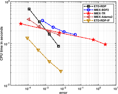
Refer to caption
Figure 3: Log-Log efficiency plot comparing ETD-RDP and ETD-RDP-IF with different second-order IMEX schemes implemented in Matlab running serial for the enzyme kinetics example using the parameters D=0.2๐ท0.2D=0.2 and T=1๐‘‡1T=1 within the unit square.

As we see in Figure 3, the ETD-RDP method has a comparable efficiency as the different second-order IMEX schemes for this problem. However, the application of dimensional splitting outperforms the IMEX schemes. Hence, the ETD-RDP-IF is the most efficient method for this enzyme kinetics example.

Note also that we tried other splitting techniques for the enzyme kinetics example, such as Strang simple splitting and Strang symmetric splitting (see [asantethesis]). It turns out that the integrating factor outperforms the other two splitting techniques (as this was also the case in [asante2]).

Now, we show in Table 2 the performance of the ETD-RDP-IF method implemented in Matlab in comparison with the Fortran implementation without and with parallelization for a variety of parameter choices for hโ„Žh and k๐‘˜k using the parameters D=0.2๐ท0.2D=0.2 and T=1๐‘‡1T=1.

k=h๐‘˜โ„Žk=h Matlab Fortran (1 thread) Fortran (3 threads)
1/10011001/100 0.16 0.14 0.06
1/20012001/200 1.20 1.19 0.48
1/40014001/400 9.76 9.87 4.54
1/80018001/800 83.26 73.80 35.81
Table 2: CPU times in seconds for the ETD-RDP-IF method implemented in Matlab and Fortran (serial and parallelized version) for the enzyme kinetics example using the parameter D=0.2๐ท0.2D=0.2 and T=1๐‘‡1T=1 within the unit square.

Although the algorithm ETD-RDP-IF is already very efficient in serial compared to other methods, it can be greatly improved first through conversion to Fortran and then through parallelization. We obtain a speed-up factor of two. Note that we list the timings of the complete program, i.e. the preparation of matrices (allocation, initialization, etc.) and the timing of the ETD-RDP-IF algorithm.

Note that one could further increase the performance of the Fortran program by using floating point arithmetic with single precision instead of double precision as used above. Using three threads and single precision arithmetic within the Fortran program, we obtain the timings 0.040.040.04, 0.330.330.33, 2.762.762.76, and 23.6523.6523.65 seconds, respectively. This gives a total speed-up factor of four compared to the Matlab implementation.

8.2 The Brusselator system

In this section, we consider the two- and three-dimensional generalization of the one-dimensional reaction-diffusion Brusselator system. For more explanations regarding the well-studied model for a hypothetical tri-molecular reaction, we refer the reader to [zegeling]*p. 526 and the references cited therein for the details and the background of this model. The system in two dimensions reads

โˆ‚u1โˆ‚tsubscript๐‘ข1๐‘ก\displaystyle\frac{\partial u_{1}}{\partial t} =\displaystyle= Dโ€‹ฮ”โ€‹u1+u12โ€‹u2โˆ’(A+1)โ€‹u1+B๐ทฮ”subscript๐‘ข1superscriptsubscript๐‘ข12subscript๐‘ข2๐ด1subscript๐‘ข1๐ต\displaystyle D\Delta u_{1}+u_{1}^{2}u_{2}-(A+1)u_{1}+B
โˆ‚u2โˆ‚tsubscript๐‘ข2๐‘ก\displaystyle\frac{\partial u_{2}}{\partial t} =\displaystyle= Dโ€‹ฮ”โ€‹u2โˆ’u12โ€‹u2+Aโ€‹u1๐ทฮ”subscript๐‘ข2superscriptsubscript๐‘ข12subscript๐‘ข2๐ดsubscript๐‘ข1\displaystyle D\Delta u_{2}-u_{1}^{2}u_{2}+Au_{1}

where the constants D๐ทD, A๐ดA, and B๐ตB are given. In our experiment, we consider the domain ฮฉ=[0,1]2ฮฉsuperscript012\Omega=[0,1]^{2} and tโˆˆ(0,2)๐‘ก02t\in(0,2) and the parameters D=2ร—10โˆ’3๐ท2superscript103D=2\times 10^{-3}, A=3.4๐ด3.4A=3.4, and B=1๐ต1B=1 as done in [asante]. We prescribe homogeneous Neumann boundary conditions for both u1subscript๐‘ข1u_{1} and u2subscript๐‘ข2u_{2}. The initial condition is given by

u1โ€‹(x,y,0)=1/2+yu2โ€‹(x,y,0)=1+5โ€‹x.formulae-sequencesubscript๐‘ข1๐‘ฅ๐‘ฆ012๐‘ฆsubscript๐‘ข2๐‘ฅ๐‘ฆ015๐‘ฅu_{1}(x,y,0)=1/2+y\,\qquad u_{2}(x,y,0)=1+5x\,.

Again, we can see in Table 3 that the estimated order of convergence agrees with the theoretical convergence order of two where we fixed h=0.0125โ„Ž0.0125h=0.0125.

k๐‘˜k ฯตโ€‹(k)ETD-RDPitalic-ฯตsubscript๐‘˜ETD-RDP\epsilon(k)_{\text{ETD-RDP}} EOC CPU Time ฯตโ€‹(k)ETD-RDP-IFitalic-ฯตsubscript๐‘˜ETD-RDP-IF\epsilon(k)_{\text{ETD-RDP-IF}} EOC CPU time
0.1000 2.3309ร—10โˆ’12.3309superscript1012.3309\times 10^{-1} 0.19429 2.3852ร—10โˆ’12.3852superscript1012.3852\times 10^{-1} 0.03740
0.0500 5.8468ร—10โˆ’25.8468superscript1025.8468\times 10^{-2} 2.00 0.38407 4.8944ร—10โˆ’24.8944superscript1024.8944\times 10^{-2} 2.28 0.06368
0.0250 1.5750ร—10โˆ’21.5750superscript1021.5750\times 10^{-2} 1.89 0.76545 1.2898ร—10โˆ’21.2898superscript1021.2898\times 10^{-2} 1.92 0.12128
0.0125 4.0884ร—10โˆ’34.0884superscript1034.0884\times 10^{-3} 1.95 1.53955 3.3223ร—10โˆ’33.3223superscript1033.3223\times 10^{-3} 1.96 0.24152
Table 3: Estimated order of convergence EOC for both the ETD-RDP and ETD-RDP-IF for the Brusselator example using the parameters D=2ร—10โˆ’3๐ท2superscript103D=2\times 10^{-3}, A=3.4๐ด3.4A=3.4, B=1๐ต1B=1, h=0.0125โ„Ž0.0125h=0.0125, and T=2๐‘‡2T=2 within the unit square. Additionally, the CPU times in seconds of the Matlab program are listed.

In Figure 4 we also show that the ETD-RDP-IF outperforms ETD-RDP and the second-order IMEX schemes IMEX-BDF2, IMEX-TR, and IMEX-Adams2 (all methods are implemented in Matlab and run serial).
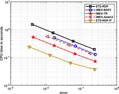
Refer to caption
Figure 4: Log-Log efficiency plot comparing ETD-RDP and ETD-RDP-IF with different second-order IMEX schemes implemented in Matlab running serial for the Brusselator example using the parameters D=2ร—10โˆ’3๐ท2superscript103D=2\times 10^{-3}, A=3.4๐ด3.4A=3.4, B=1๐ต1B=1, and T=2๐‘‡2T=2 within the unit square.

The CPU timings can be greatly improved through the Fortran implementation and additionally through parallelization. The CPU timings are listed in Table 4.

k=h๐‘˜โ„Žk=h Matlab Fortran (1 thread) Fortran (3 threads)
1/10011001/100 0.51 0.36 0.16
1/20012001/200 3.87 3.32 1.60
1/40014001/400 34.05 28.99 13.92
1/80018001/800 286.06 190.75 114.19
Table 4: CPU times in seconds for the ETD-RDP-IF method implemented in Matlab and Fortran (serial and parallelized version) for the Brusselator example using the parameters D=2ร—10โˆ’3๐ท2superscript103D=2\times 10^{-3}, A=3.4๐ด3.4A=3.4, B=1๐ต1B=1, and T=2๐‘‡2T=2.

As we can see, the serial Fortran program is faster than the Matlab program as expected. The parallelized version is almost twice as fast as the serial version.

Finally, we also consider the three-dimensional Brusselator example on the domain ฮฉ=[0,1]3ฮฉsuperscript013\Omega=[0,1]^{3} with the same initial and boundary conditions and parameters as in test problem 4 within [bhatt]. Precisely, we use homogeneous Neumann boundary conditions and as initial conditions u1โ€‹(x,y,z,0)=1+sinโก(2โ€‹ฯ€โ€‹x)โ€‹sinโก(2โ€‹ฯ€โ€‹y)โ€‹sinโก(2โ€‹ฯ€โ€‹z)subscript๐‘ข1๐‘ฅ๐‘ฆ๐‘ง012๐œ‹๐‘ฅ2๐œ‹๐‘ฆ2๐œ‹๐‘งu_{1}(x,y,z,0)=1+\sin(2\pi x)\sin(2\pi y)\sin(2\pi z) and u2โ€‹(x,y,z,0)=3subscript๐‘ข2๐‘ฅ๐‘ฆ๐‘ง03u_{2}(x,y,z,0)=3. The parameters are D=0.02๐ท0.02D=0.02, A=1๐ด1A=1, B=2๐ต2B=2, and T=5๐‘‡5T=5. The spatial and time step are given by h=1/10โ„Ž110h=1/10 and k=1/1000๐‘˜11000k=1/1000. In Figure 5, we show a 2D slice through the 3D domain of u1subscript๐‘ข1u_{1} and u2subscript๐‘ข2u_{2} for z=1๐‘ง1z=1 and the final time T=5๐‘‡5T=5.

Refer to caption
Refer to caption
Figure 5: The concentration profiles of u1subscript๐‘ข1u_{1} and u2subscript๐‘ข2u_{2} for z=1๐‘ง1z=1 at T=5๐‘‡5T=5 using the parameters D=0.02๐ท0.02D=0.02, A=1๐ด1A=1, B=2๐ต2B=2, h=1/10โ„Ž110h=1/10 and k=1/1000๐‘˜11000k=1/1000.

The two plots agree with the theory of the terminal behavior of the equation proposed in the paper [twizell] since 1โˆ’A+B2โ‰ฅ01๐ดsuperscript๐ต201-A+B^{2}\geq 0 holds. Note that the Matlab program needs 2.872.872.87 seconds to compute the result. The serial and parallelized Fortran version only need 1.271.271.27 and 0.650.650.65 seconds, respectively. In Figure 6 (left) we also show the solutions u1subscript๐‘ข1u_{1} and u2subscript๐‘ข2u_{2} at the point (0.3,0.3,0.3)0.30.30.3(0.3,0.3,0.3) for the time interval [0,5]05[0,5] using the same parameters as before. Additionally, we also show in Figure 6 (right) the solutions u1subscript๐‘ข1u_{1} and u2subscript๐‘ข2u_{2} at the point (1/3,1/3,1/3)131313(1/3,1/3,1/3) for the time interval [0,40]040[0,40] using the parameters D=0.02๐ท0.02D=0.02, A=3๐ด3A=3, B=1๐ต1B=1, h=1/10โ„Ž110h=1/10 and k=1/1000๐‘˜11000k=1/1000. Hence, the equation 1โˆ’A+B2โ‰ฅ01๐ดsuperscript๐ต201-A+B^{2}\geq 0 is violated.

Refer to caption
Refer to caption
Figure 6: Left: profile of u1subscript๐‘ข1u_{1} and u2subscript๐‘ข2u_{2} at the point (1/3,1/3,1/3)131313(1/3,1/3,1/3) for the time interval [0,5]05[0,5] using the parameters D=0.02๐ท0.02D=0.02, A=1๐ด1A=1, B=2๐ต2B=2, h=1/10โ„Ž110h=1/10 and k=1/1000๐‘˜11000k=1/1000. Right: profile of u1subscript๐‘ข1u_{1} and u2subscript๐‘ข2u_{2} at the point (1/3,1/3,1/3)131313(1/3,1/3,1/3) for the time interval [0,40]040[0,40] using the parameters D=0.02๐ท0.02D=0.02, A=3๐ด3A=3, B=1๐ต1B=1, h=1/10โ„Ž110h=1/10 and k=1/1000๐‘˜11000k=1/1000.

As expected, the values approach B๐ตB and A/B๐ด๐ตA/B (here 222 and 1/2121/2) as t๐‘กt increases, since 1โˆ’A+B2โ‰ฅ01๐ดsuperscript๐ต201-A+B^{2}\geq 0 is satisfied. However, if we choose A=3๐ด3A=3 and B=1๐ต1B=1, then 1โˆ’A+B2โ‰ฅ01๐ดsuperscript๐ต201-A+B^{2}\geq 0 is violated and we obtain an oscillatory solution. This again is in agreement with [twizell] that the solution does not converge to a fixed concentration. The plots shown in Figure 6 are also in agreement with Figures 10 and 11 within [bhatt].

8.3 The complex Ginzburg-Landau equation on a periodic domain

The complex Ginzburg-Landau equation [ginzburg] has been extensively studied in the physics community. It describes a variety of phenomena such as non-linear waves to second-order phase transitions, from superconductivity, superfluidity, and Bose-Einstein condensation to liquid crystals and strings in field theory (see [aranson] for a general overview). The complex Ginzburg-Landau equation is given by

โˆ‚uโˆ‚t=u+(1+iโ€‹ฮฑ)โ€‹ฮ”โ€‹uโˆ’(1+iโ€‹ฮฒ)โ€‹uโ€‹|u|2๐‘ข๐‘ก๐‘ข1i๐›ผฮ”๐‘ข1i๐›ฝ๐‘ขsuperscript๐‘ข2\frac{\partial u}{\partial t}=u+(1+\mathrm{i}\alpha)\Delta u-\left(1+\mathrm{i}\beta\right)u\left|u\right|^{2}

where the constants ฮฑ๐›ผ\alpha and ฮฒ๐›ฝ\beta are given real-valued parameters describing linear and non-linear dispersion, respectively. Here, the prescribed initial condition is given by a normal random field with mean zero and standard deviation one, but could also be a smooth function such as a series of Gaussian pulses. The boundary condition is assumed to be periodic. Hence, it fits into the format (2) with s=1๐‘ 1s=1, D=1+iโ€‹ฮฑ๐ท1i๐›ผD=1+\mathrm{i}\alpha, and fโ€‹(u)=uโˆ’(1+iโ€‹ฮฒ)โ€‹uโ€‹|u|2๐‘“๐‘ข๐‘ข1i๐›ฝ๐‘ขsuperscript๐‘ข2f(u)=u-\left(1+\mathrm{i}\beta\right)u\left|u\right|^{2}.

For our experiment, we consider the domain ฮฉ=[0,200]2ฮฉsuperscript02002\Omega=[0,200]^{2} and tโˆˆ(0,100)๐‘ก0100t\in(0,100) and the parameters ฮฑ=0๐›ผ0\alpha=0 and ฮฒ=1.3๐›ฝ1.3\beta=1.3. For the discretization in space, we use p=400๐‘400p=400 (h=1/2โ„Ž12h=1/2). For the time step, we use k=1/20๐‘˜120k=1/20. To produce the result that is shown in Figure 7, we need about 96 seconds with our implementation in Matlab without any parallelization.
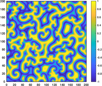
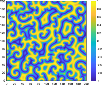
Refer to caption
Refer to caption
Figure 7: Real (left image) and imaginary part (right image) of the solution of the complex Ginzburg-Landau equation on the periodic domain ฮฉ=[0,200]2ฮฉsuperscript02002\Omega=[0,200]^{2} for time T=100๐‘‡100T=100 with the parameters ฮฑ=0๐›ผ0\alpha=0, ฮฒ=1.3๐›ฝ1.3\beta=1.3, p=400๐‘400p=400, and k=1/20๐‘˜120k=1/20 using a standard normal random field as initial condition.

Thus, we obtain a comparable performance with the numerical method that is based on Fourier spatial discretization and a fourth-order exponential time differencing Runge-Kutta (ETDRK4) method that is usually faster than the standard finite difference scheme (see [kassamtrefethen]). However, special attention has to be drawn to the time stepping in Fourier space to avoid aliasing effects. The implementation of the Fourier spectral ETDRK4 method in Matlab with the same set of parameters as above needs only 28 seconds (see p. 11 for the Matlab implementation within [kassam]). Of course, we have only compared the timing and not the approximation quality of the solution as one should. Further, our method is L๐ฟL-stable in comparison to the EDTRK4 and one could create a situation where ETD-RDP-IF outperforms ETDRK4 in the sense of approximation quality or more precisely in the sense of CPU time versus accuracy.

In sum, we obtain a stable solution although the initial data are non-smooth. We obtain similar solution patterns, when we use smooth initial boundary conditions such as a series of Gaussian pulses in the form uโ€‹(x,y,0)=eโˆ’((xโˆ’50)2+(yโˆ’50)2)/1000โˆ’eโˆ’((xโˆ’100)2+(yโˆ’100)2)/1000+eโˆ’((xโˆ’100)2+(yโˆ’50)2)/1000๐‘ข๐‘ฅ๐‘ฆ0superscriptesuperscript๐‘ฅ502superscript๐‘ฆ5021000superscriptesuperscript๐‘ฅ1002superscript๐‘ฆ10021000superscriptesuperscript๐‘ฅ1002superscript๐‘ฆ5021000u(x,y,0)=\mathrm{e}^{-((x-50)^{2}+(y-50)^{2})/1000}-\mathrm{e}^{-((x-100)^{2}+(y-100)^{2})/1000}+\mathrm{e}^{-((x-100)^{2}+(y-50)^{2})/1000} with the same set of parameters as before. We again need about 96 (95.6595.6595.65 to be precise) seconds in Matlab without parallelization to produce the images shown in Figure 8.
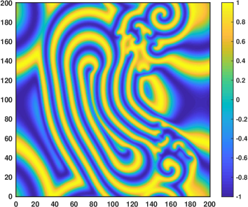
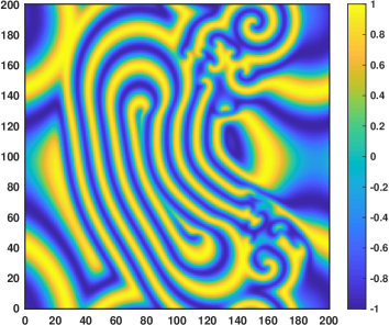
Refer to caption
Refer to caption
Figure 8: Real (left image) and imaginary part (right image) of the solution of the complex Ginzburg-Landau equation on the periodic domain ฮฉ=[0,200]2ฮฉsuperscript02002\Omega=[0,200]^{2} for time T=100๐‘‡100T=100 with the parameters ฮฑ=0๐›ผ0\alpha=0, ฮฒ=1.3๐›ฝ1.3\beta=1.3, p=400๐‘400p=400, and k=1/20๐‘˜120k=1/20 using a series of Gaussian pulses field as initial condition.

The serial Fortran version needs 4.994.994.99 seconds and the parallelized Fortran version needs only 2.762.762.76 seconds. Refer also to the last row in Table 5.

p๐‘p hโ„Žh Matlab Fortran (1 thread) Fortran (3 threads)
505050 444 1.24 1.23 0.51
100100100 222 5.17 4.95 2.04
200200200 111 23.11 20.85 10.34
400400400 1/2121/2 95.65 86.66 53.98
Table 5: CPU times in seconds for the ETD-RDP-IF method implemented in Matlab and Fortran (serial and parallelized version) for the Ginzburg-Landau example on periodic domain ฮฉ=[0,200]2ฮฉsuperscript02002\Omega=[0,200]^{2} using the parameters ฮฑ=0๐›ผ0\alpha=0, ฮฒ=1.3๐›ฝ1.3\beta=1.3, k=1/20๐‘˜120k=1/20, and T=100๐‘‡100T=100.

A similar situation arises when we consider the three-dimensional case. The ETDRK4 using a spectral method needs only 27 seconds in Matlab with the parameters ฮฑ=0๐›ผ0\alpha=0, ฮฒ=1.3๐›ฝ1.3\beta=1.3, p=50๐‘50p=50 (h=2โ„Ž2h=2), and k=1/20๐‘˜120k=1/20 for time T=100๐‘‡100T=100 and ฮฉ=[0,100]3ฮฉsuperscript01003\Omega=[0,100]^{3} whereas our method in Matlab (without any parallelization) needs about 119 seconds, which is longer as expected due to the second-versus-fourth order of the schemes. The serial and parallelized Fortran program need 108.21108.21108.21 and 57.8757.8757.87 seconds, respectively.

We now consider ฮฉ=[0,200]3ฮฉsuperscript02003\Omega=[0,200]^{3} with the same parameters as before and increase the parameter p๐‘p to 200200200. That means, we have 8,000,00080000008,000,000 spatial discretization points. Gaussian pulses as initial condition of the form uโ€‹(x,y,z,0)=eโˆ’((xโˆ’50)2+(yโˆ’50)2+(zโˆ’50)2)/1000โˆ’eโˆ’((xโˆ’100)2+(yโˆ’100)2+(zโˆ’100)2)/1000๐‘ข๐‘ฅ๐‘ฆ๐‘ง0superscriptesuperscript๐‘ฅ502superscript๐‘ฆ502superscript๐‘ง5021000superscriptesuperscript๐‘ฅ1002superscript๐‘ฆ1002superscript๐‘ง10021000u(x,y,z,0)=\mathrm{e}^{-((x-50)^{2}+(y-50)^{2}+(z-50)^{2})/1000}-\mathrm{e}^{-((x-100)^{2}+(y-100)^{2}+(z-100)^{2})/1000} are used, which yields Figure 9.

Refer to caption
Refer to caption
Figure 9: Real (left image) and imaginary part (right image) of the solution of the complex Ginzburg-Landau equation on the periodic domain ฮฉ=[0,200]3ฮฉsuperscript02003\Omega=[0,200]^{3} for time T=100๐‘‡100T=100 with the parameters ฮฑ=0๐›ผ0\alpha=0, ฮฒ=1.3๐›ฝ1.3\beta=1.3, p=200๐‘200p=200, and k=1/20๐‘˜120k=1/20 using a series of Gaussian pulses field as initial condition.

The Matlab program needs 9673.139673.139673.13 seconds whereas the serial and parallelized Fortran program need 8260.918260.918260.91 and 5287.645287.645287.64 seconds, respectively. Refer also to the last row in Table 6.

p๐‘p hโ„Žh Matlab Fortran (1 thread) Fortran (3 threads)
505050 444 119.61 108.37 57.94
100100100 222 1033.63 912.41 585.91
200200200 111 9673.13 8260.91 5287.64
Table 6: CPU times in seconds for the ETD-RDP-IF method implemented in Matlab and Fortran (serial and parallelized version) for the Ginzburg-Landau example on periodic domain ฮฉ=[0,200]3ฮฉsuperscript02003\Omega=[0,200]^{3} using the parameters ฮฑ=0๐›ผ0\alpha=0, ฮฒ=1.3๐›ฝ1.3\beta=1.3, k=1/20๐‘˜120k=1/20, and T=100๐‘‡100T=100.

8.4 Schrรถdinger equation

The Schrรถdinger equation [schroedinger] is a linear PDE and it describes a state function of a quantum-mechanical system (see for example [griffiths] for more details). However, in this section, we consider an extension of it. Precisely, we focus on the d๐‘‘d-dimensional non-linear cubic Schrรถdinger equation of the form

iโ€‹ฮจt+ฮ”โ€‹ฮจ=qโ€‹(|ฮจ|2)โ€‹ฮจ,๐ฑโˆˆ[0,1]d,tโˆˆ(0,T)formulae-sequenceisubscriptฮจ๐‘กฮ”ฮจ๐‘žsuperscriptฮจ2ฮจformulae-sequence๐ฑsuperscript01๐‘‘๐‘ก0๐‘‡\mathrm{i}\Psi_{t}+\Delta\Psi=q\left(|\Psi|^{2}\right)\Psi\,,\qquad\mathbf{x}\in[0,1]^{d}\,,\quad t\in(0,T) (27)

with given initial condition ฮจ0โ€‹(๐ฑ)=ฮจโ€‹(๐ฑ,0)subscriptฮจ0๐ฑฮจ๐ฑ0\Psi_{0}(\mathbf{x})=\Psi(\mathbf{x},0) and homogeneous Neumann boundary condition. Here, q๐‘žq is a given function of |ฮจ|2superscriptฮจ2|\Psi|^{2}. The wave function ฮจโ€‹(๐ฑ,t)ฮจ๐ฑ๐‘ก\Psi(\mathbf{x},t) can be written as vโ€‹(๐ฑ,t)+iโ€‹wโ€‹(๐ฑ,t)๐‘ฃ๐ฑ๐‘กi๐‘ค๐ฑ๐‘กv(\mathbf{x},t)+\mathrm{i}w(\mathbf{x},t) and hence, we obtain the coupled system of equations

vt+ฮ”โ€‹wsubscript๐‘ฃ๐‘กฮ”๐‘ค\displaystyle v_{t}+\Delta w =qโ€‹(v2+w2)โ€‹wabsent๐‘žsuperscript๐‘ฃ2superscript๐‘ค2๐‘ค\displaystyle=\,\,\,\,q(v^{2}+w^{2})w
wtโˆ’ฮ”โ€‹vsubscript๐‘ค๐‘กฮ”๐‘ฃ\displaystyle w_{t}-\Delta v =โˆ’qโ€‹(v2+w2)โ€‹vabsent๐‘žsuperscript๐‘ฃ2superscript๐‘ค2๐‘ฃ\displaystyle=-q(v^{2}+w^{2})v

which can be written as

(vtwt)+(01โˆ’10)โ€‹(ฮ”โ€‹vฮ”โ€‹w)=qโ€‹(u2+w2)โ€‹(01โˆ’10)โ€‹(vw).matrixsubscript๐‘ฃ๐‘กsubscript๐‘ค๐‘กmatrix0110matrixฮ”๐‘ฃฮ”๐‘ค๐‘žsuperscript๐‘ข2superscript๐‘ค2matrix0110matrix๐‘ฃ๐‘ค\begin{pmatrix}v_{t}\\ w_{t}\end{pmatrix}+\begin{pmatrix}0&1\\ -1&0\end{pmatrix}\begin{pmatrix}\Delta v\\ \Delta w\end{pmatrix}=q(u^{2}+w^{2})\begin{pmatrix}0&1\\ -1&0\end{pmatrix}\begin{pmatrix}v\\ w\end{pmatrix}.

By setting ๐ฎ=(vw)โ€‹ย andย D=(01โˆ’10)๐ฎmatrix๐‘ฃ๐‘คย andย Dmatrix0110\mathbf{u}=\begin{pmatrix}v\\ w\end{pmatrix}\text{ and }\textbf{D}=\begin{pmatrix}0&1\\ -1&0\end{pmatrix} we can rewrite the system as

๐ฎt+๐ƒโ€‹ฮ”โ€‹๐ฎ=qโ€‹(|๐ฎ|2)โ€‹๐ƒ๐ฎsubscript๐ฎ๐‘ก๐ƒฮ”๐ฎ๐‘žsuperscript๐ฎ2๐ƒ๐ฎ\mathbf{u}_{t}+\mathbf{D}\Delta\mathbf{u}=q(|\mathbf{u}|^{2})\mathbf{D}\mathbf{u}

which fits into the format (2). However, note that D is not a diagonal matrix. Using the approximation of the Laplacian as in Example 1 and Example 2, one can again verify similarly to Lemma 2 that the dimensional splitting commutes and hence the ETD-RDP-IF method can be used.

First, we present numerical results for the one-dimensional non-linear cubic Schrรถdinger equation of the form (see also [Bratsos2015]*Section 4)

iโ€‹ฮจt+ฮจxโ€‹x+|ฮจ|2โ€‹ฮจ=0,โˆ’L0<x<L1,0<t<Tformulae-sequenceformulae-sequenceisubscriptฮจ๐‘กsubscriptฮจ๐‘ฅ๐‘ฅsuperscriptฮจ2ฮจ0subscript๐ฟ0๐‘ฅsubscript๐ฟ10๐‘ก๐‘‡\mathrm{i}\Psi_{t}+\Psi_{xx}+|\Psi|^{2}\Psi=0\,,\qquad-L_{0}<x<L_{1}\,,\quad 0<t<T (28)

with initial condition

ฮจโ€‹(x,0)=2โ€‹aโ€‹expโ€‹(iโ€‹c2โ€‹x)โ€‹sechโ€‹(aโ€‹x)ฮจ๐‘ฅ02๐‘Žexpi๐‘2๐‘ฅsech๐‘Ž๐‘ฅ\Psi(x,0)=\sqrt{2a}\,\mathrm{exp}\left(\mathrm{i}\,\frac{c}{2}x\right)\mathrm{sech}(\sqrt{a}x)

and homogeneous Neumann boundary condition. The function

ฮจโ€‹(x,t)=2โ€‹aโ€‹expโ€‹[iโ€‹(c2โ€‹xโˆ’{c24โˆ’a}โ€‹t)]โ€‹sechโ€‹(aโ€‹(xโˆ’cโ€‹t))ฮจ๐‘ฅ๐‘ก2๐‘Žexpdelimited-[]๐‘–๐‘2๐‘ฅsuperscript๐‘24๐‘Ž๐‘กsech๐‘Ž๐‘ฅ๐‘๐‘ก\Psi(x,t)=\sqrt{2a}\,\mathrm{exp}\left[i\left(\frac{c}{2}x-\left\{\frac{c^{2}}{4}-a\right\}t\right)\right]\mathrm{sech}(\sqrt{a}(x-ct))\,

satisfies the Schrรถdinger equation and the Neumann boundary condition as |x|๐‘ฅ|x| approaches infinity. The total mass Mโ€‹(t)๐‘€๐‘กM(t) and energy Eโ€‹(t)๐ธ๐‘กE(t) of the wave function are given by

Mโ€‹(t)๐‘€๐‘ก\displaystyle M(t) =โˆซโ„|ฮจโ€‹(x,t)|2โ€‹dx,absentsubscriptโ„superscriptฮจ๐‘ฅ๐‘ก2differential-d๐‘ฅ\displaystyle=\int_{\mathbb{R}}|\Psi(x,t)|^{2}\,\mathrm{d}x\,,
Eโ€‹(t)๐ธ๐‘ก\displaystyle E(t) =โˆซโ„(|ฮจxโ€‹(x,t)|2โˆ’12โ€‹|ฮจโ€‹(x,t)|4)โ€‹dx,absentsubscriptโ„superscriptsubscriptฮจ๐‘ฅ๐‘ฅ๐‘ก212superscriptฮจ๐‘ฅ๐‘ก4differential-d๐‘ฅ\displaystyle=\int_{\mathbb{R}}\left(|\Psi_{x}(x,t)|^{2}-\frac{1}{2}|\Psi(x,t)|^{4}\right)\;\mathrm{d}x\,,

respectively. For the purpose of numerically verifying the conservation of these quantities, we approximate the integrals by the trapezoidal rule (as in [Bratsos2015]*Section 4.4)

Mโ€‹(tn)๐‘€subscript๐‘ก๐‘›\displaystyle M(t_{n}) โ‰ˆh2โ€‹[|๐”0n|2+2โ€‹โˆ‘i=1p|๐”in|2+|๐”p+1n|2]absentโ„Ž2delimited-[]superscriptsuperscriptsubscript๐”0๐‘›22superscriptsubscript๐‘–1๐‘superscriptsuperscriptsubscript๐”๐‘–๐‘›2superscriptsuperscriptsubscript๐”๐‘1๐‘›2\displaystyle\approx\frac{h}{2}\left[|\mathbf{U}_{0}^{n}|^{2}+2\sum_{i=1}^{p}|\mathbf{U}_{i}^{n}|^{2}+|\mathbf{U}_{p+1}^{n}|^{2}\right]
Eโ€‹(tn)๐ธsubscript๐‘ก๐‘›\displaystyle E(t_{n}) โ‰ˆh2โ€‹[โˆ’12โ€‹(|๐”0n|4+|๐”p+1n|4)+2โ€‹โˆ‘i=1p(|๐”i+1nโˆ’๐”iโˆ’1n2โ€‹h|2โˆ’12โ€‹|๐”in|4)].absentโ„Ž2delimited-[]12superscriptsuperscriptsubscript๐”0๐‘›4superscriptsuperscriptsubscript๐”๐‘1๐‘›42superscriptsubscript๐‘–1๐‘superscriptsuperscriptsubscript๐”๐‘–1๐‘›superscriptsubscript๐”๐‘–1๐‘›2โ„Ž212superscriptsuperscriptsubscript๐”๐‘–๐‘›4\displaystyle\approx\frac{h}{2}\left[-\frac{1}{2}(|\mathbf{U}_{0}^{n}|^{4}+|\mathbf{U}_{p+1}^{n}|^{4})+2\sum_{i=1}^{p}\left(\left|\frac{\mathbf{U}_{i+1}^{n}-\mathbf{U}_{i-1}^{n}}{2h}\right|^{2}-\frac{1}{2}|\mathbf{U}_{i}^{n}|^{4}\right)\right]\,.

For the numerical results we used the parameters a=0.01๐‘Ž0.01a=0.01, c=0.1๐‘0.1c=0.1, T=108๐‘‡108T=108, h=1/2โ„Ž12h=1/2, and ฮ”โ€‹t=1/100ฮ”๐‘ก1100\Delta t=1/100 within the interval [L0,L1]=[โˆ’80,100]subscript๐ฟ0subscript๐ฟ180100[L_{0},L_{1}]=[-80,100]. A plot of the exact solution (defined on โ„โ„\mathbb{R}) and the approximated solution (defined on [โˆ’80,100]80100[-80,100]) with computing time less than five seconds in Matlab reveals visually no difference and agrees with the one given in [Bratsos2015]*Figure 4.1. The exact values for Mโ€‹(0)๐‘€0M(0) and Mโ€‹(108)๐‘€108M(108) can be obtained by basic integration techniques from calculus. They are both 2/5=0.4250.42/5=0.4. Numerically, we obtain 0.399โ€‰999โ€‰954โ€‰123โ€‰2810.3999999541232810.399\,999\,954\,123\,281 and 0.399โ€‰999โ€‰954โ€‰128โ€‰0360.3999999541280360.399\,999\,954\,128\,036, respectively. For the energy Eโ€‹(0)๐ธ0E(0) and Eโ€‹(108)๐ธ108E(108), we obtain the exact value โˆ’1/3000โ‰ˆโˆ’0.000โ€‰333โ€‰333โ€‰333โ€‰333130000.000333333333333-1/3000\approx-0.000\,333\,333\,333\,333. We obtain numerically โˆ’0.000โ€‰336โ€‰760โ€‰546โ€‰2940.000336760546294-0.000\,336\,760\,546\,294 and โˆ’0.000โ€‰336โ€‰768โ€‰976โ€‰7960.000336768976796-0.000\,336\,768\,976\,796. Hence, the mass and the energy are conserved asymptotically for the approximated solution obtained via ETD-RDP-IF.

Next, we consider the two-dimensional Schrรถdinger equation within the unit square and the function qโ€‹(|๐ฎ|2)=Bโ€‹(x,y)+Cโ€‹(x,y)โ€‹|๐ฎ|2๐‘žsuperscript๐ฎ2๐ต๐‘ฅ๐‘ฆ๐ถ๐‘ฅ๐‘ฆsuperscript๐ฎ2q(|\mathbf{u}|^{2})=B(x,y)+C(x,y)|\mathbf{u}|^{2} with Bโ€‹(x,y)=(1โˆ’2โ€‹ฯ€2)โ€‹(1โˆ’cos2โก(ฯ€โ€‹x)โ€‹cos2โก(ฯ€โ€‹y))๐ต๐‘ฅ๐‘ฆ12superscript๐œ‹21superscript2๐œ‹๐‘ฅsuperscript2๐œ‹๐‘ฆB(x,y)=(1-2\pi^{2})(1-\cos^{2}(\pi x)\cos^{2}(\pi y)) and Cโ€‹(x,y)=(1โˆ’2โ€‹ฯ€2)๐ถ๐‘ฅ๐‘ฆ12superscript๐œ‹2C(x,y)=(1-2\pi^{2}). The exact solution is given by ฮจโ€‹(x,y,t)=eโˆ’iโ€‹tโ€‹cosโก(ฯ€โ€‹x)โ€‹cosโก(ฯ€โ€‹y)ฮจ๐‘ฅ๐‘ฆ๐‘กsuperscriptei๐‘ก๐œ‹๐‘ฅ๐œ‹๐‘ฆ\Psi(x,y,t)=\mathrm{e}^{-\mathrm{i}t}\cos(\pi x)\cos(\pi y) (see also [mehdi]*p. 754). We use the parameters T=1๐‘‡1T=1, k=0.0125๐‘˜0.0125k=0.0125, and h=1/78โ„Ž178h=1/78 to create the same plot as in [mehdi]*Figure 5 within one second. Note that we obtain similar timing improvements for the parallelized Fortran version in comparison to the serial Matlab program as in the Brusselator example. For some recent results on more complex domains, we refer the reader to [speck].

9 Conclusion

In this article, we have combined the second-order exponential time differencing method (ETD) of second-order with approximating the matrix exponential through (non-Padรฉ) rational approximation having real simple and distinct poles (RDP) and the integrating factor (IF) dimensional splitting technique to obtain the second-order L๐ฟL-stable ETD-RDP-IF scheme in two and three dimensions. With this scheme, one can solve non-linear reaction-diffusion equations with either Dirichlet, Neumann, or periodic boundary conditions in either two or three dimensions. The new scheme outperforms other second-order IMEX schemes such as IMEX-BDF2, IMEX-TR, and IMEX-Adams2 as well as ETD-RDP. The excellent performance for 2D and above all 3D examples can be further enhanced through the conversion from Matlab to Fortran. Using basic parallelization techniques increases the efficiency further. The source code is available under the link

https://github.com/kleefeld80/ETDRDPIF

In the future, we intend to extend these ideas to develop methods with higher order. Additionally, incorporating an adaptive time selection procedure to these methods might further increase the performance. As an alternative one might want to consider and apply parallel-in-time procedures (see for example [Gander2015] for an overview).

Acknowlegement

The collaboration of the authors arose in Cรกdiz, Spain during the international Conference on Computational and Mathematical Methods in Science and Engineering (CMMSEโ€™19). We would like to thank the organizer, Jesรบs Vigo-Aguiar, for valuable support and encouragement.

References