How Does BN Increase Collapsed Neural Network Filters?

Abstract

Improving sparsity of deep neural networks (DNNs) is essential for network compression and has drawn much attention. In this work, we disclose a harmful sparsifying process called filter collapse, which is common in DNNs with batch normalization (BN) and rectified linear activation functions (e.g. ReLU, Leaky ReLU). It occurs even without explicit sparsity-inducing regularizations such as $L_{1}$. This phenomenon is caused by the normalization effect of BN, which induces a non-trainable region in the parameter space and reduces the network capacity as a result. This phenomenon becomes more prominent when the network is trained with large learning rates (LR) or adaptive LR schedulers, and when the network is finetuned. We analytically prove that the parameters of BN tend to become sparser during SGD updates with high gradient noise and that the sparsifying probability is proportional to the square of learning rate and inversely proportional to the square of the scale parameter of BN. To prevent the undesirable collapsed filters, we propose a simple yet effective approach named post-shifted BN (psBN), which has the same representation ability as BN while being able to automatically make BN parameters trainable again as they saturate during training. With psBN, we can recover collapsed filters and increase the model performance in various tasks such as classification on CIFAR-10 and object detection on MS-COCO2017.

1 Introduction

Neural network sparsification as a method to accelerate its inference speed has drawn much attention in the past years [1, 2, 3, 4, 5, 6]. Commonly adopted methods for pruning either enforce an additional explicit $L_{1}$ [7] or $L_{0}$ [8] regularization during training.

In this study, we find that training a standard deep network such as ResNet [9] or VGG-BN [10] can also generate structured network parameter sparsity without the above sparsity-imposing regularizers. The weight parameters of certain convolution kernels and the following BN parameters all become negligible (absolute value $<10^{-7}$) after training. We also find that one requisite for such phenomenon is the usage of batch normalization (BN)[11] before non-linear activation such as ReLU [12, 13] and Leaky ReLU [14].

As a successful normalization technique, BN helps in different aspects in both training [11, 15] and generalization [16]. However, its behavior in inducing a sparsified network has not been recorded in the literature.

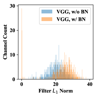
It is found in this work that the reason for such phenomenon lies in the combination of BN and rectified nonlinear activation functions like ReLU. When the network with BN is retrained on the same dataset using the same strategy, a much sparser network in the filter level is generated compared to the network without BN (Fig. 1a).

This is because the normalization in BN implies a steady frozen zone in its parameter space of scale $\gamma$ and bias $\beta$. Once in the frozen space, the parameters will only be squashed to 0 by weight decay. This process is illustrated by the trace of BN parameters in Figure 1b. We show such sparsification also exists in other network normalization methods as well, such as instance normalization [17].

(a)

(b)

Figure 1: (a) The $L_{1}$ norm distribution of convolutional filters of one layer for VGG11 with and without BN. (b) The trace of BN scale ($\gamma$) and bias ($\beta$) parameters of one layer in ResNet-20 during the second round training on CIFAR-10. (Collapsed filters run from the outside to the origin point)

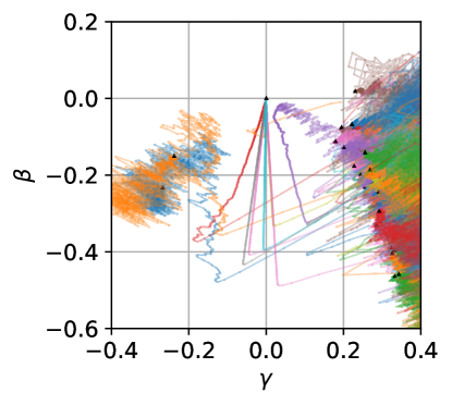
Some other contributing factors to the network sparsification are also discussed here. It is observed that a relatively large learning rate (LR), weight decay (WD) also contribute to the filter sparsity level. More importantly, iterative LR annealing schedules is also found to increase the sparsity in the network. This implies the wide-spread existence of collapsed filters in the network generated by iterative “warmup” [18] schedules and common transfer learning tasks by network finetuning such as object detection [19].

With the finding of increased sparsity due to BN + ReLU, a natural question is whether the sparsity is favorable for the network. Several recent works treated the sparsity as a windfall in network training since it automatically generates a pruned network [20, 21]. However, in this work, we show that the accuracy of the sparsified network only matches that using uniform channel pruning, suggesting detrimental effects of the collapsed filters.

Moreover, we also analytically model the transition probability of BN parameters to the non-trainable regions for the first time. The BN parameters would always tend to become sparser when the noise level of the gradient is large, which is common in training with large learning rates or small batches. From our statistical model, we also conclude that the sparsifying probability is proportional to the square of learning rate and inversely proportional to the square of the scale parameter of BN. These findings have been testified with experiments on training deep networks using natural datasets and help explain the increasing sparsity as a network is trained with iterative annealing of learning rate.

To escape the non-trainable region caused by normalization and ReLU, we propose a simple yet effective method that only shifts the original BN by a small positive constant number. By utilizing this technique, the aforementioned non-trainable region is proved non-stable, and collapsed filters would eventually be reactivated again. The representation of the new normalization layer is mathematically equivalent to the original one, and is able to increase the performance due to its removal of parameter sparsity of BN. With this technique, a network is found to be able to defend common settings that would trigger collapsed filters. Apart from classification tasks, we also testify its usefulness in tasks with network parameters transfer by finetuning, such as object detection on MS-COCO2017. A steady increase of mAP on a standard RetinaNet is also observed.

This paper contributes in the following aspects:

• We find that the common combination of BN and ReLU induces collapsed filters in a network and that the normalization operation in BN is the source of the stable non-tranable region.

• The sparsification due to BN + ReLU is found to actually harm both training, generalization and transferability, which is undesirable for tasks aiming at higher performance.

• A mathematical model is provided to explain the sparsification and predicts that the network will keep sparsing during training with strong noises.

• We propose a post-shifted BN (psBN) as an easy approach that not only avoids the network non-trainable region but still keeps sparse representations of ReLU;

2 Related Work

2.1 Network pruning

The sparsified representation of ReLU has inspired direct pruning strategies on the feature map[22, 23, 24] in the literature.However, there is a major difference between the collapsed filters found in this study from precedent pruning methods utilizing ReLU sparsification. Whether or not BN induced sparsity is favorable for the loss function is still unknown. In the current work, it is found that the network parameters almost always tend to drop to the non-trainable zone, especially at a large LR or with great gradient uncertainty. Therefore, instead of facilitating sparsity in network parameters, we present an appeal for cautious treatment of the collapsed filters.

2.2 Dying ReLU

Dying ReLU refers to a situation where the input of ReLU is smaller than 0 and becomes non-trainable. Several recent studies have investigated the dying probability with network depth[25]. The ReLU-related network sparsity in neural networks has also been noticed by two contemporary works[21, 20], yet with no special attention to batch normalization. The sparsification change with different hyper-parameters such as LR, weight decay and training algorithms was experimentally analyzed in [21]. [20] also identified the increased weight sparsity with Adam optimizer by relating it to the larger convergence rate of Adam under only $L_{2}$ regularization when weights are non-trainable by the target loss function. Both of these two studies also tried to utilize it as a pruning methods. However, in this study we doubt the efficacy of collapsed ReLU as a pruning method by both comparing the performance of the sparsified model and random pruning method and analytically illustrate the sparsing probability of parameters with different distributions.

2.3 Effects of BN in deep networks

BN usually receives much applause due to its boosting performance in various tasks[11, 26]. It is generally thought to be able to allow a larger learning rate [27], smooth the loss landscape [15] and increase network generalization ability [16]. On the other hand, [28] also noted a side effect of BN. It was derived that at random initialization, the inter-sample correlation due to BN could lead to gradient explosion, leading to non-trainable deep networks. Although the non-trainable filters due to BN+ReLU in this work may be reminiscent of gradient explosion due to BN, there are some key differences both empirically and theoretically. (1) The analysis in [28] mainly applies for random initialization, when BN becomes ill-conditioned. However, the network with BN at random initialization is still trainable in this study. On the contrary, filter-level sparsity occurs when LR suddenly increases at convergence, where the gradients tend to be small instead of exploding. (2) The cause of filter sparsity in this study is analyzed from the stabilization effect of BN on feature distribution. Whereas the cause of gradient explosion in BN is the inter-sample correlation when batch size is small.

3 How does BN+ReLU make network parameters sparse?

3.1 Experimental setup

We study the filter collapsing phenomenon on CIFAR-10 dataset [29] using three architectures with different depth and paradigm: ResNet-20, ResNet-56 [9] and VGG16-BN [30]. All networks are trained using SGD with momentum $0.9$ and cosine annealing learning rate schedule [18] with initial learning rate $0.1$ for 100 epochs. We choose batch size $128$ and weight decay $5\mathrm{e}{-4}$ throughout the experiments. Data augmentation is performed as in [9] unless specified. We consider structured sparsity in this study, and a convolutional filter is considered as pruned when its corresponding scaling parameter in the following BN layer is smaller than a certain threshold. The threshold is chosen to be $1\mathrm{e}{-3}$ in our experiments since pruning at this level does not bring observable performance degradation (accuracy $\pm 0.03\%$) to the models.

3.2 Sparsity in warm restart

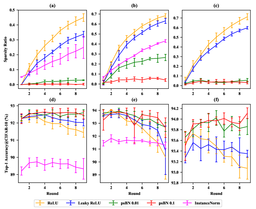
We consider training a network for multiple rounds, where a round refers to one stage of cosine annealing of the learning rate. For each network architecture, we use $5$ different random seeds and train the network for $9$ rounds, and calculate the sparsity (i.e. the percentage of reduced FLOPS [7]) and validation accuracy at the end of each round. It is worthy of noting that the relatively large total training budget mainly helps manifest the sparsification effect of BN+ReLU, and experiments using much shorter training steps (40 epochs per round and 5 rounds in total) have also been conducted (see later discussions). The result is shown in Fig. 3 (the orange curve). It is clear from the figure that after each round of training, the sparsity of a network is increased. Surprisingly, the removable channels also have a clear distinction with other channels in the parameter space. Figure 1a shows the distribution of the $L_{1}$ norm of convolutional filters for a snapshot after round 3, the distribution has an isolated peak at $0$ which resembles the parameter distribution of a network trained with explicit sparsifying regularizers such as the LASSO [31].

Accompanying the increasing sparsity is the deteriorating validation performance. As proposed in [18], performing restart during optimization can improve the performance of the final network. Presumably, training the model for more rounds should not harm its performance. Our results show that this is not the case with the commonly used BN $+$ ReLU network, since more filters will collapse and the network capacity will be decreased.

3.3 The effect of random labels

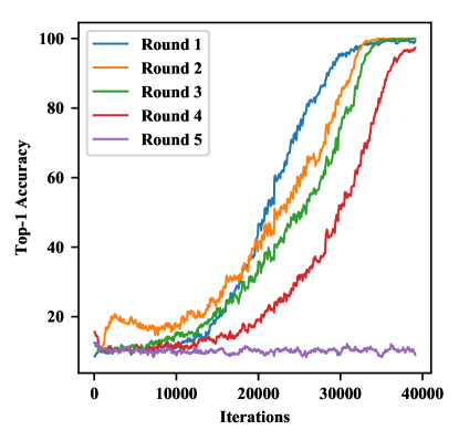
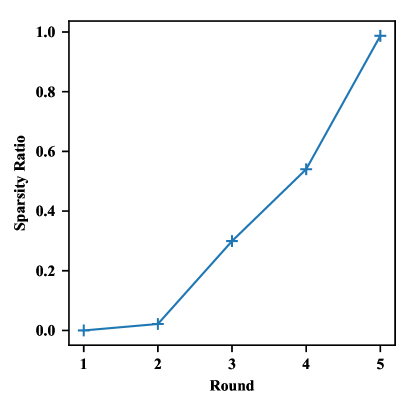
In this subsection, we try to exclude the impact of a specific dataset by training a network with random labels. We take the CIFAR-10 dataset and randomly shuffle the image labels before the training starts. Note that the correspondence between an image and its label is fixed but kept random. A network trained using such dataset will have minimal, if any, dependence on the latent structure of the data distribution, and a high performance network has to ”remember” the dataset. We train ResNet-20 on CIFAR-10 with random labels and the training loss of each round is shown in Fig. 2a. In the first four rounds, the network fits the training data quite well, while its sparsity keeps increasing after each round of training (Fig. 2b). The presence of filter collapse on the random dataset shows that this phenomenon is not specific to a particular dataset.

(a)

(b)

Figure 2: (a) Training curve of ResNet-20 on CIFAR-10 with random labels. The network fails to fit the training data during the fifth round due to filter collapse. (b) Sparsity ratio of ResNet-20 on CIFAR-10 with random labels. The sparsity increases with each round of restart.

3.4 The effect of BN on filter collapse

We study the effect of batch normalization on network sparsity caused by filter collapse. The distribution of the filter $L_{1}$ norm for a specific layer in VGG11-BN at the end of the second round is shown in Fig. 1a. The filter sparsity only becomes evident with the presence of BN. The distribution for VGG11-BN has a characteristic high peak at zero while the distribution of VGG11 does not have noticeable concentration near zero. Therefore collapsed filters should be related with BN. Moreover, the filter-level sparsity is not unique to BN but also observed in other normalizations, e.g. instance normalization, suggesting a similar role played by the normalization during the process.

3.5 The effect of non-linear activation on filter collapse

To study the effect of non-linear activation on filter collapse, we replace ReLU with Leaky ReLU with slope $0.01$ at the negative range. Leaky ReLU has a finite activation at the negative range. However, from the change in both network sparsity and accuracy change with different rounds of training (Fig. 3), we observe that Leaky ReLU only has a marginal effect in avoiding collapsed filters, which also coincides with the conclusion in [21]. We have also tested the case where ReLU activations is removed after each BN layer of VGG11-BN, resulting in a deep linear network. The linear network is trained using the same strategy as before, and sparsity is barely observed ($<1\%$) at the end of the second round of training. Therefore, the phenomenon of collapsed filters is likely to be caused by a combined effect of BN and reticified activation functions.

3.6 Other factors contributing to filter collapse

As shown in Fig. 3, collapsed filters only appear starting from the second round of training. Since the network architecture is invariant during learning rate restart, there must be other factors contributing to this phenomenon.

Figure 3: Sparsity and accuracy comparison of different normalization-activation combinations. The horizontal axis is the number of training rounds. Top row: sparsity ratio for (a) ResNet-20; (b) ResNet-56; (c) VGG16-BN. Bottom row: top-1 accuracy on CIFAR-10 for (d) ResNet-20; (e) ResNet-56; (f) VGG16-BN.

Filter selectivity?

A reasonable hypothesis is that since the network has already converged at a good local minimum at the end of the first round of training, training the network for another round allows the network to select and prune unimportant filters by itself. However, this assumption is disproved by our experiments. We consider a trained network at the end of round 1 and randomly shuffle its parameters within the same parameter tensor. If a network can self-prune based on a loss-aware selectivity metric (e.g. Fisher information, Hessian, etc), decorrelating network weights and loss should result in much fewer sparsity. Surprisingly, training the trained-and-shuffled network for another round still induces collapsed filters. This observation weakens the relation between network sparsification and loss-based selectivity. In fact, the performance degradation observed even suggests that a trained model may not be a good initialization at all.

Distribution of $\gamma$

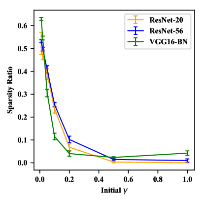
A common practice for initializing BN parameters is to set the scale to $1$ and the bias to $0$. This is different from the distribution of $\gamma$s when the model is converged at the end of round 1, where most of the $\gamma$s are much smaller than $1$. We hypothesize that the smaller initial value of $\gamma$s for subsequent rounds encourages the filters to collapse. This is experimentally confirmed by setting $\gamma$s to smaller values at the first round of training. The sparsity of different networks for different values of initial $\gamma$s is shown in Fig. 5b. The sparsity of the network increases significantly when the initialization of $\gamma$s is decreased.

Figure 4: Comparison of network pruning methods for ResNet-20 on CIFAR-10. We compare uniform filter ablation with methods that collapse filters using (1) larger LR; (2) adaptive LR method (Adam); (3) retrain for multiple rounds.

3.7 Effectiveness of filter collapse for network pruning

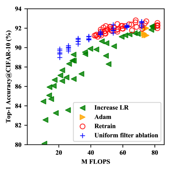
Since filter collapse introduces removable convolutional channels in the network, it is natural to consider exploiting this for network pruning. We compare the following sparsity-inducing methods: training the network for multiple rounds (retrain), using large learning rate (Increase LR), using Adam optimizer [21] and uniformly ablating all convolutional filters (Uniform filter ablation). All methods are applied to pruning ResNet-20 on CIFAR-10. (Detailed training settings can be seen in the supplementary material)

The accuracy and computational cost (in FLOPS) for the pruned network using four different methods is shown in figure 4. Interestingly, no method performs better than the naive Uniform filter ablation method. This comparison suggests that pruning the collapsed filters is not better than pruning random filters.

4 Why does BN + ReLU make network parameters sparse?

In this section, we aim to find the conditions that drive a neuron to the non-activation range. We found that the majority of transition process of the BN parameters to the non-trainable range happens at the first several hundreds of steps when LR suddenly increases. The noise brought by the increased LR becomes so strong that it may even overwhelm the gradient propagated from the target loss function. Therefore, it would be helpful to find the relation between the transition probability of BN parameters to the non-trainable region and the noise level of the gradient. Here we use the activation probability of the neuron $\mathbb{P}(\gamma\hat{x}+\beta>0)$ to also represent possibility for a set of parameters $\gamma$ and $\beta$ to be trainable. The BN parameters are updated at each SGD step and changes the neuron activation probability.

4.1 Notations and Assumptions

In batch normalization that is applied in convolutional neural networks, the average statistics is calculated for a single filter without considering inter-channel correlation. Therefore it would ease the calculation by dropping the neuron index and focus on the behavior of a single neuron. The activation magnitude after ReLU is $y=\operatorname{ReLU}(\gamma\hat{x}+\beta)$. $\hat{x}$ is the normalized output after a linear kernel $\hat{x}=\frac{{\mathbf{w}}{{}^{\mkern-1.5mu\mathsf{T}}}\cdot{\mathbf{x}}-\mu_{\mathcal{{B}}}}{\sigma_{\mathcal{{B}}}}$, where $\mu_{\mathcal{{B}}}$ and $\sigma_{\mathcal{{B}}}$ are the batch average and standard deviation of the linear output ${\mathbf{w}}{{}^{\mkern-1.5mu\mathsf{T}}}\cdot{\mathbf{x}}$. Despite the form of a single neuron activation, it is able to represent behavior of all neurons in the same layer by assigning $\gamma$ and $\beta$ as variables drawn from specific unknown distributions $P(\gamma)$ and $P(\beta)$. Even though the distribution of input layer ${\mathbf{x}}$ is unknown, the distribution of ${\mathbf{w}}{{}^{\mkern-1.5mu\mathsf{T}}}\cdot{\mathbf{x}}$ reaches Gaussian-alike especially as the number of input channels $N\rightarrow\infty$ due to the central limit theorem. This applies for deeper layers in a neural network. Let $\phi(\hat{x})$ represent the probability distribution function of $\hat{x}$ and let $\Phi(\hat{x})$ be its cumulative distribution.

4.2 Neuron activation probability

With the above treatments and assumptions, we are able to calculate the probability of a activating neuron. The probability that the layer is activated given parameters $\gamma$ and $\beta$ is defined as $\mathbb{P}(\gamma\hat{x}+\beta>0)$ Note that we assume that $\gamma>0$ throughout the whole section without loss of generality since its behavior is symmetric for $\gamma<0$. After defining the variables and their probability density functions, we can examine the model $y=\operatorname{ReLU}(\gamma\hat{x}+\beta)$ and its properties. Given $\eta$ and $L$ as the learning rate and the loss function, then the update rules are:

$$\Delta\gamma =-\eta\hat{x}\frac{\partial L}{\partial y}H(\gamma\cdot\hat{x}+\beta)$$ (1)

$$\Delta\beta =-\eta\frac{\partial L}{\partial y}H(\gamma\cdot\hat{x}+\beta)$$

where $\frac{\partial L}{\partial y}$ is the gradient to the activation output and $H(\cdot)$ is the Heaviside step function. Here we focus our attention to the “local” behavior of the current layer, which cares only the gradient correlation between the neighboring two layers while treating the gradients from higher levels as independent.Moreover, as stated above, the sparsification process is observed to happen when the noise overwhelms its true gradients. Therefore we treat $\frac{\partial L}{\partial y}$ as an independent gradient with zero mean and variance $c^{2}$, where $c$ is a constant number. Then $\Delta\gamma$, $\Delta\beta$ are both random variables depending on $\frac{\partial L}{\partial y}$. After a single step of update with stochastic gradient descent (SGD), BN parameters now become $\gamma^{\prime}=\gamma+\Delta\gamma,\beta^{\prime}=\beta+\Delta\beta$.

The probability that the layer is activated before the update is

$$\mathbb{P}(y>0)=\mathbb{P}((\hat{x}>-\frac{\beta}{\gamma}))=1-\Phi(-\frac{\beta}{\gamma})=\Phi(\frac{\beta}{\gamma})$$ (2)

Therefore, the expectation for $\mathbb{P}(y>0)$ is $\mathbb{E}_{\gamma,\beta}(\Phi(\frac{\beta}{\gamma}))$. After the update, the new expected probability for the layer activation is $\mathbb{E}_{\gamma\prime,\beta^{\prime}}(\Phi(\frac{\beta^{\prime}}{\gamma^{\prime}}))$. We show the expected probability that the layer is activated becomes smaller during SGD updates by proposing the following theorem, which proves that the expected activation probability will tend to decrease at each step of learning, i.e.

$$\mathbb{E}_{\gamma^{\prime},\beta^{\prime}}(\Phi(\frac{\beta^{\prime}}{\gamma^{\prime}}))<\mathbb{E}_{\gamma,\beta}(\Phi(\frac{\beta}{\gamma}))$$

Theorem 1

Assume the update of BN parameters $\gamma$ and $\beta$ update according to Eq. (1), further assume that $\hat{x}\sim N(0,1)$, then

$$\mathbb{E}_{\gamma^{\prime},\beta^{\prime}}(\Phi(\frac{\beta^{\prime}}{\gamma^{\prime}}))=\mathbb{E}_{\gamma,\beta}(\Phi(\frac{\beta}{\gamma}))+\frac{\eta^{2}c^{2}}{2}\int_{\mathbb{R}}\frac{1}{\gamma^{2}}P(\gamma)J(\gamma)d\gamma$$ (3)

where

$$J(\gamma)=\int_{\mathbb{R}}K(\frac{\beta}{\gamma})P(\beta)d\beta$$ (4)

and

$$K(\frac{\beta}{\gamma})=((\frac{\beta}{\gamma})^{4}-2)\phi(\frac{\beta}{\gamma})^{2}+(\frac{\beta}{\gamma}-(\frac{\beta}{\gamma})^{3})\phi(\frac{\beta}{\gamma})\Phi(\frac{\beta}{\gamma})$$ (5)

Further assume $\beta$ follows an even distribution, $J(\gamma)$ is then a function that is always negative and hence $\mathbb{E}_{\gamma^{\prime},\beta^{\prime}}(\Phi(\frac{\beta^{\prime}}{\gamma^{\prime}}))<\mathbb{E}_{\gamma,\beta}(\Phi(\frac{\beta}{\gamma}))$

We provide detailed proof in the supplementary. The above theorem provides a proof that neurons are prone to be less activated during each updating step at a high noise level of gradients, and it provides some key insights towards understanding the sparsification process.

Learning rate and gradient noise

According the Eq. (3), it is noticed that the decrease of neuron activation probability is proportional to $\eta^{2}c^{2}$, where $\eta$ is the learning rate and $c$ is the variance of the gradients in regards to the output. This relation reveals that the noise in gradients might drives BN parameters into the non-trainable region, and that large learning rate behaves similarly with to noise level.

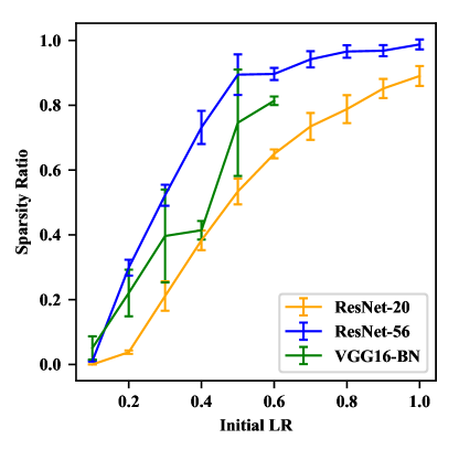
To study the relation between learning rate and the level of filter collapse, we train networks on CIFAR-10 with initial learning rate in range $[0.1,1]$. The resulting sparsity is shown in figure 5a. It can be seen that larger learning rate induces more collapsed filters.

Initialization of $\gamma$

For a general initialization technique of BN, $\beta$ is initialized to be $0$. In this scenario, it is easy to prove that $J(\gamma)=C$, where $C$ is a negative constant. Therefore, the decrease of neuron activation is proportional to $\frac{1}{\gamma^{2}}$. Fig. 5b shows the change of network that the sparsity level $\gamma$ initialization value. Therefore, the conclusions from Theorem. 1 are verified experimentally.

(a)

(b)

Figure 5: The sparsity level change with (a) LR and (b) $\gamma$ initialization

4.3 Weight decay

The above analysis discusses the transition probability of BN parameters to the non-trainable region. It is also found that weight decay does more than an equivalent $L_{2}$ regularization that helps avoid overfitting. Weight decay is also able to collect all non-trainable parameters to zero. Moreover, under a constant weight decay factor $\lambda$. It would be easy to derive that the ratio $\frac{\beta}{\gamma}$ would maintain the original value throughout the decay. It indicates an almost intact non-activating status for these two parameters and both parameters in BN finally approaches 0, representing a true sparsified filter.

5 Proposed method of avoiding sparsity

In the above sections, BN + ReLU has been shown to induce collapsed filters under various conditions. Filters always tend to drop to the non-trainable region regardless of the training target when learning rate is large. Therefore, avoiding the non-trainable region is desirable in order to fully stretch the training ability of each parameter in the network. A direct solution would be adding a regularization term to the training loss. However, adding regularizations highly relies on prior knowledge of the distribution of network parameters. In this study, we propose a more elegant method that adopt a post-shifted BN that can solve the collapsing filter problem more elegantly.

$$y=\text{BN}(\hat{x})+\alpha=\gamma\cdot\frac{\hat{x}-\mu_{\mathcal{{B}}}}{\sqrt{\sigma_{\mathcal{{B}}}^{2}+\epsilon}}+\beta+\alpha\quad\quad(\alpha>0)\\$$ (6)

where the definition of all parameters are the same as in the original batch normalization [11] except that a small positive constant $\alpha$ is added to prevent collapsed filters. Since $\alpha$ is a mere constant, using it to shift BN is mathematically equivalent to the original one. However, the BN parameters would behave differently as they fall into the non-trainable region at a step. To demonstrate the difference, we assume there exist a BN filter at time step $t$ satisfying $\frac{\beta^{t}+\alpha}{|\gamma^{t}|}=C^{t}\ll 0$, indicating a collapsed filter. After a single step of weight decay ($\Delta\gamma^{t}=-\eta\lambda\gamma^{t}$ and $\Delta\beta^{t}=-\eta\lambda\beta^{t}$, where $\lambda$ is weight decay strength), it can be easy to show $C^{t+1}=C^{t}+\frac{\eta\lambda}{1-\eta\lambda}\frac{\alpha}{|\gamma|}>C^{t}$. Therefore, The collapsed filter would sooner be reactivated instead of decaying directly to $0$. On the other hand, the $\alpha$ should be small enough to avoid a strong prior on the bias of BN. It has been tested on different tasks that $\alpha=0.1$ works stably for different tasks and is thus mostly adopted in the following discussion.

5.1 Avoiding sparsity in CIFAR-10 training

In this section, we show that using psBN can prevent filter collapse for networks trained with cyclic learning rate on CIFAR-10 dataset. As for the experimental setup in Fig. 3, we replace the BN layers of a network with psBN using $\alpha=0.1$, and compare psBN against the BN + ReLU/Leaky ReLU baselines. As shown in the figure, psBN inhibits filter collapse and performance degradation significantly especially in the later rounds.

5.2 Avoiding sparsity in snapshot ensemble

As proposed in [32], snapshots of a network at the end of each round of learning rate decay can be ensembled to boost the test time performance. Following the original setup, the total training budget is constrained to 200 epochs and is divided into 5 cyclic rounds. Then the models of the last three snapshots are ensembled to reach higher performance than the model directly trained in a single LR decay using the same training budget (200 epochs). The baseline top-1 accuracy of ensembles for initial LR equaling 0.1 & 0.2 are 94.27 & 94.68 from the original paper. As seen from Table 1, the network sparsity also nearly monotonically increases for a standard snapshot training. Thus the representation power of the ensembled model is not fully utilized due to the filter collapse phenomenon. This problem is alleviated by psBN, which evidently outperforms the baseline of snapshot ensemble.

Table 1: Snapshot Ensemble [32] training for ResNet-110 on CIFAR-10. Each cell is in the format psBN(baseline).

InitLR	Metric	#1	#2	#3	#4	#5	Ensemble
0.2	Val acc (%)	92.38(92.23)	93.51(93.51)	93.92(93.94)	94.00(94.01)	94.29(94.10)	94.86(94.63)
0.2	Sparsity (%)	0.4(0.4)	1.0(8.1)	2.8(16.6)	4.5(24.5)	5.3(31.6)	N/A
0.1	Val acc(%)	88.86(91.26)	92.81(92.93)	93.49 (93.18)	94.05 (93.67)	94.43(93.75)	94.75(94.12)
0.1	Sparsity (%)	0.2 (0.0)	0.2(0.0)	0.8(1.2)	0.6(2.8)	0.8(3.8)	N/A

5.3 Avoiding sparsity in COCO-2017 Object Detection

From previous discussions, iterative LR annealing would result in more sparsity to the network and avoiding the undesirable sparsity brings a performance increase. Extending the observation and our theoretical proof to a broader span, one would find that a sudden learning rate increase also exist in various transfer learning tasks including object detection, where neural networks which are often pretrained on ImageNet are finetuned again. Therefore, a certain degree of sparsity would also occur during the finetuning process.

We experiment on the RetinaNet[19] baseline using a ResNet-50 [9] backbone. When examining the distribution of BN weights of the model trained with standard BN+ReLU, we also found sparsified weights in deep layers, suggesting possibly collapsed ReLU.

Table 2 shows the comparison between our proposed shifted BN and both the reported and our implemented baseline. The shifted BN shows a steady increase over the performance of RetinaNet across different image scales.

Table 2: Post-shifted BN (psBN) performance on MS-COCO2017 dataset. The baseline performance of RetinaNet[19] reported in the original paper is also listed in the bracket following the AP value of our implementation.

Image scale	APbbox (baseline)	APbbox (psBN)
500	32.7(32.5)	33.4
800	35.8(35.7)	36.4

6 Conclusion

In this study, we report a side effect of the common combination between BN and ReLU. The normalization layer in BN induces a stable non-trainable region in BN parameters due to the increased collapsing ReLU. Apart from the larger learning rate (LR) and adaptive LR optimization schedules that also contribute to more sparse parameters, we also found that this phenomenon is more manifest with multiple rounds of annealing LR, and that the induced sparsity also exist in other normalizations such as instance normalization. The phenomenon is attributed to the stable non-trainable zone for parameters induced by the normalization in BN. Instead of being potential to be a pruning method, the sparsity in the network is found to be harmful to the network performance. We also analytically prove that the network parameters tend to become more sparse at each SGD update. A post-shifted BN (psBN) is also proposed to help network escape the undesirable sparsity. It is advantageous in having the same representation ability with BN and being able to make parameters retrainable again. Its efficacy have been testified on both CIFAR-10 and MS-COCO2017 datasets with stable increase in the performance.

References

- [1] Song Han, Huizi Mao, and William J. Dally. Deep compression: Compressing deep neural network with pruning, trained quantization and huffman coding. In ICLR, 2016.
- [2] Song Han, Jeff Pool, Sharan Narang, Huizi Mao, Enhao Gong, Shijian Tang, Erich Elsen, Peter Vajda, Manohar Paluri, John Tran, Bryan Catanzaro, and William J. Dally. DSD: Dense-Sparse-Dense Training for Deep Neural Networks. arXiv:1607.04381 [cs], July 2016. arXiv: 1607.04381.
- [3] Yihui He, Xiangyu Zhang, and Jian Sun. Channel pruning for accelerating very deep neural networks. In Proceedings of the IEEE International Conference on Computer Vision, pages 1389–1397, 2017.
- [4] Huizi Mao, Song Han, Jeff Pool, Wenshuo Li, Xingyu Liu, Yu Wang, and William J. Dally. Exploring the Regularity of Sparse Structure in Convolutional Neural Networks. arXiv:1705.08922 [cs, stat], May 2017. arXiv: 1705.08922.
- [5] H. Ide and T. Kurita. Improvement of learning for CNN with ReLU activation by sparse regularization. In 2017 International Joint Conference on Neural Networks (IJCNN), pages 2684–2691, May 2017.
- [6] Dongwoo Lee, Sungbum Kang, and Kiyoung Choi. ComPEND: Computation Pruning through Early Negative Detection for ReLU in a Deep Neural Network Accelerator. In Proceedings of the 2018 International Conference on Supercomputing - ICS ’18, pages 139–148, Beijing, China, 2018. ACM Press.
- [7] Ariel Gordon, Elad Eban, Ofir Nachum, Bo Chen, Hao Wu, Tien-Ju Yang, and Edward Choi. MorphNet: Fast & Simple Resource-Constrained Structure Learning of Deep Networks. In 2018 IEEE/CVF Conference on Computer Vision and Pattern Recognition, pages 1586–1595, Salt Lake City, UT, June 2018. IEEE.
- [8] Christos Louizos, Max Welling, and Diederik P. Kingma. Learning Sparse Neural Networks through $L_0$ Regularization. arXiv:1712.01312 [cs, stat], December 2017. arXiv: 1712.01312.
- [9] Kaiming He, Xiangyu Zhang, Shaoqing Ren, and Jian Sun. Deep residual learning for image recognition. In Proceedings of the IEEE conference on computer vision and pattern recognition, pages 770–778, 2016.
- [10] Karen Simonyan and Andrew Zisserman. Very deep convolutional networks for large-scale image recognition. arXiv preprint arXiv:1409.1556, 2014.
- [11] Sergey Ioffe and Christian Szegedy. Batch Normalization: Accelerating Deep Network Training by Reducing Internal Covariate Shift. In PMLR, pages 448–456, June 2015.
- [12] Xavier Glorot, Antoine Bordes, and Yoshua Bengio. Deep sparse rectifier neural networks. In Proceedings of the fourteenth international conference on artificial intelligence and statistics, pages 315–323, 2011.
- [13] Richard LT Hahnloser. On the piecewise analysis of networks of linear threshold neurons. Neural Networks, 11(4):691–697, 1998.
- [14] Andrew L Maas, Awni Y Hannun, and Andrew Y Ng. Rectifier nonlinearities improve neural network acoustic models. In Proc. icml, volume 30, page 3, 2013.
- [15] Shibani Santurkar, Dimitris Tsipras, Andrew Ilyas, and Aleksander Madry. How does batch normalization help optimization? In Advances in Neural Information Processing Systems, pages 2483–2493, 2018.
- [16] Ping Luo, Xinjiang Wang, Wenqi Shao, and Zhanglin Peng. Towards understanding regularization in batch normalization. 2018.
- [17] Dmitry Ulyanov, Andrea Vedaldi, and Victor Lempitsky. Instance normalization: The missing ingredient for fast stylization. arXiv preprint arXiv:1607.08022, 2016.
- [18] Ilya Loshchilov and Frank Hutter. Sgdr: Stochastic gradient descent with warm restarts. arXiv preprint arXiv:1608.03983, 2016.
- [19] Tsung-Yi Lin, Priya Goyal, Ross Girshick, Kaiming He, and Piotr Dollár. Focal loss for dense object detection. In Proceedings of the IEEE international conference on computer vision, pages 2980–2988, 2017.
- [20] Atsushi Yaguchi, Taiji Suzuki, Wataru Asano, Shuhei Nitta, Yukinobu Sakata, and Akiyuki Tanizawa. Adam Induces Implicit Weight Sparsity in Rectifier Neural Networks. arXiv:1812.08119 [cs, stat], December 2018. arXiv: 1812.08119.
- [21] Dushyant Mehta, Kwang In Kim, and Christian Theobalt. On implicit filter level sparsity in convolutional neural networks. In Proceedings of the IEEE Conference on Computer Vision and Pattern Recognition, pages 520–528, 2019.
- [22] Tailin Liang, Lei Wang, Shaobo Shi, and John Glossner. Dynamic runtime feature map pruning. arXiv preprint arXiv:1812.09922, 2018.
- [23] Xingyu Liu, Jeff Pool, Song Han, and William J. Dally. Efficient Sparse-Winograd Convolutional Neural Networks. arXiv:1802.06367 [cs], February 2018. arXiv: 1802.06367.
- [24] Jiayu Dong, Huicheng Zheng, and Lina Lian. Activation-based weight significance criterion for pruning deep neural networks. In International Conference on Image and Graphics, pages 62–73. Springer, 2017.
- [25] Lu Lu, Yeonjong Shin, Yanhui Su, and George Em Karniadakis. Dying relu and initialization: Theory and numerical examples. arXiv preprint arXiv:1903.06733, 2019.
- [26] Christian Szegedy, Vincent Vanhoucke, Sergey Ioffe, Jon Shlens, and Zbigniew Wojna. Rethinking the inception architecture for computer vision. In Proceedings of the IEEE conference on computer vision and pattern recognition, pages 2818–2826, 2016.
- [27] Nils Bjorck, Carla P Gomes, Bart Selman, and Kilian Q Weinberger. Understanding batch normalization. In Advances in Neural Information Processing Systems, pages 7694–7705, 2018.
- [28] Greg Yang, Jeffrey Pennington, Vinay Rao, Jascha Sohl-Dickstein, and Samuel S Schoenholz. A mean field theory of batch normalization. arXiv preprint arXiv:1902.08129, 2019.
- [29] Alex Krizhevsky, Vinod Nair, and Geoffrey Hinton. The cifar-10 dataset. online: http://www. cs. toronto. edu/kriz/cifar. html, 55, 2014.
- [30] K. Simonyan and A. Zisserman. Very deep convolutional networks for large-scale image recognition. CoRR, abs/1409.1556, 2014.
- [31] Robert Tibshirani. Regression shrinkage and selection via the lasso. JOURNAL OF THE ROYAL STATISTICAL SOCIETY, SERIES B, 58:267–288, 1994.
- [32] Gao Huang, Yixuan Li, Geoff Pleiss, Zhuang Liu, John E. Hopcroft, and Kilian Q. Weinberger. Snapshot ensembles: Train 1, get M for free. CoRR, abs/1704.00109, 2017.