A CNN With Multiscale Convolution for Hyperspectral Image Classification using Target-Pixel-Orientation scheme

Abstract

Presently, CNN is a popular choice to handle the hyperspectral image classification challenges. In spite of having such large spectral information in Hyper-Spectral Image(s) (HSI), it creates a curse of dimensionality. Also, large spatial variability of spectral signature adds more difficulty in classification problem. Additionally, scarcity of training examples is a bottleneck in using a CNN. In this paper, a novel target-patch-orientation method is proposed to train a CNN based network. Also, we have introduced a hybrid of 3D-CNN and 2D-CNN based network architecture to implement band reduction and feature extraction methods, respectively. Experimental results show that our method outperforms the accuracies reported in the existing state of the art methods.

I Introduction

Hyperspectral image (HSI) classification has received considerable attention in recent years for a variety of application using neural network-based techniques. Hyperspectral imagery has several hundreds of contiguous narrow spectral bands from the visible to the infrared frequency in the entire electromagnetic spectrum. However, processing such a large number of spectral dimension suffers from the curse of dimensionality. Also, a few properties of the dataset bring challenges in the classification of HSIs, such as 1) limited training examples, and 2) large spatial variability of spectral signature. In general, contiguous spectral bands may contain some redundant information which leads to the Hughes phenomenon [1]. It causes accuracy drop in classification when there is an imbalance between the high number of spectral channels and scarce training examples. Conventionally, dimension-reduction techniques are used to extract a suitable spectral feature. For instance, Independent Component Discriminant Analysis (ICDA) [2] has been used to find statistically independent components. It uses ICA with the assumption that at most one component has a Gaussian distribution. ICA uses higher order statistics to compute uncorrelated components compared to the PCA [3] which uses the covariance matrix. A few other non-linear techniques quadratic discriminant analysis [4], kernel-based methods [5], etc., are also employed to handle non-linearity in HSIs. However, extracted features in the reduced dimensional space may not be optimal for classification. HSI classification task gets more complicated with the following facts: i) spectral signature of objects belonging to the same class may be different, and ii) the spectral signature of objects belonging to different classes may be the same. Therefore, only spectral components may not be sufficient to provide discriminating features for classification. Recent studies prove that incorporation of spatial context along with spectral components improves classification task considerably. There are two ways of exploiting spatial and spectral information for classification. In the first approach, spatial and spectral information are processed separately and then combined at the decision level [32, 19]. The second strategy uses joint representation of spectral-spatial features [31, 33, 30, 34]. In this paper, a novel joint representation of spectral-spatial features has been proposed. Our technique supersedes the accuracy of classification compared to the state of the art techniques.

In the literature, 1-D [30], 2-D [31], and 3-D [20] CNN based architectures are well-known for HSI classification. Also, hybridisation of different CNN-type architecture is employed [21]. 1D-CNNs use pixel-pair strategy [30] which combines a set of pairs of training samples. Each pair is constructed using all permutations of training pixels under consideration. This set not only reveals the neighborhood of the observed pixel but also increases the training samples. Yet, it can not use full power of spatial information in hyper-spectral image classification. It completely ignores neighborhood profile. In general, 2-D and 3-D CNN based approaches are more suitable in such a scenario. However, there are many other architectures, e.g., Deep Belief Network [22, 23, 24, 25], Autoencoders [26, 27, 28, 29] which provide efficient solution to the hyperspectral image classification problem. Multi-scale convolution is widely popular in literature for exploring complex spatial context. In most cases, outputs of different kernels are either concatenated [42, 43] or summed [31] together and further processed for feature extraction and classification. However, there exists no study on whether concatenating a large number of filter banks of different scales result in optimum classification. In the present context, we are more interested in scrutinizing various CNN architectures for the current problem. In general, a few core components are available for making any CNN architecture. For example, convolution, pooling, batch-normalization [40], and activation layers. In practice, there are various ways of using convolution mechanism. A few of them are very popular, namely, point convolution, group convolution, depth-wise separable convolution [39], etc. Similarly, there is a variation to the pooling mechanism, namely, adaptive pooling [41]. Recently, many mid-level components are developed, e.g., an inception module which integrates outputs of multi-scale convolutions. Mid-level components are sequentially combined to make a large network, such as, VGG [36], GoogleNet [37], etc. Additionally, a skip architecture [38] proves to be a successful way of making a very deep network to deal with the vanishing gradient problem. Hyperspectral image classification is still an interesting and challenging problem where the effectiveness of various core components of CNN and their arrangement to resolve the classification problem, needs to be studied. To summarize, our work is motivated by the following observations.

1. Incorporating spatial and spectral feature may achieve better classification accuracy for hyperspectral images. Hence, a strategy is needed to combine spatial and spectral information.

2. Due to complex reflectance property in HSI, pixels of same class may have different spectral signature and pixels of different class may have similar spectral signature. Spatial neighborhood plays a key role in improving classification accuracies in such scenario. However, the neighborhood of a pixel at class boundary appears different compared to the non-boundary pixels. It is observed that non-boundary pixels include more pixels from the same class. However, the neighborhood of boundary pixels include pixels of different classes. Our strategy aims to bring similar neighborhood for the boundary and non-boundary pixels which belong to the same class.

3. Substantial spectral information brings redundancy, and also taking all spectral bands together decreases the performance of classification. Hence, band reduction is required in hyperspectral image classification.

4. A suitable network architecture is needed to handle the problems stated above such that the network can be trained in an end to end manner.

In this paper, we present a CNN architecture which performs three major tasks in a pipeline of processing, such as, :1) band reduction, 2) feature extraction, and 3) classification. The first block of processing uses point-wise 3-D convolution layers. For feature extraction, we use multi-scale convolution module. In our work, we propose two architectures for feature extraction which eventually lead to two different CNN architectures. In the first architecture, we use an inception module with four parallel convolution structures for feature extraction. Additionally, we use similar multi-scale convolutions in inception like structure but with a different arrangement. The second architecture extracts finer contextual information compared to the first one. We feed the extracted features to a fully connected layer to form the high-level representation. We train our network in an end to end manner by minimizing cross-entropy loss using Adam optimizer. Our proposed architecture gives a state of the art performance without any data augmentation on three benchmark HSI classification datasets. Besides this new architecture, we propose a way to incorporate spatial information along with the spectral one. It not only covers the neighborhood profile for a given window, but also it observes the change of neighborhood by shifting its current window. We observe that this process appears to be more beneficial towards the boundary location compared to the a single window neighborhood system. The contribution of this paper can be summarized as follows:

1. A novel technique to obtain a joint representation of spatial and spectral features has been proposed. The design is aimed at improving classification accuracy at the boundary location of each class.

2. A novel end to end shallow and wider neural network has been proposed, which is a hybridization of 3-D CNN with 2-D-CNN. This hybrid structure does band reduction followed by a discriminating feature extraction. Also, we have shown two different arrangements of similar multi-scale convolutional layers to extract distinctive features.

Section II-A gives a detailed description of the proposed classification framework, including the technique of inclusion of the spatial information. Performance and comparisons among the proposed networks and current state of the art methods are presented in Section III. This paper is concluded in Section IV.

II PROPOSED CLASSIFICATION FRAMEWORK

The proposed classification framework shown in Fig 1 mainly consists of three tasks: i) organizing a target-pixel-orientation model using available training samples, ii) constructing a CNN architecture to extract uncorrelated spectral information, and iii) learning spatial correlation with neighboring pixels.

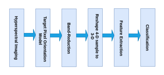
Figure 1: Flowchart of the proposed classification framework

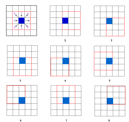
Figure 2: Example of Target-Patch-Orientation Model

II-A Target-Pixel-Orientation Model for Training Samples

Consider a hyperspectral data set $H$ with $d$ spectral bands. We have $N$ labeled samples denoted as $P=\{p_{i}\}_{i=1}^{N}$ in an $R^{d\times 1}$ feature space and class labels $y_{i}\in\{1,2,\cdots,C\}$ where $C$ is the number of class. Let $n_{c}$ be the number of available labeled samples in the $c^{th}$ class and $\sum_{c=1}^{C}n_{c}=N$. We propose a Target-Pixel-Orientation (TPO) scheme. In this scheme, we consider a $k\times k$ window whose center pixel is the target pixel. We select eight neighbors of the target pixel by simply shifting the window into eight different directions in a clockwise manner. Fig 2 shows one example of how we prepare eight neighboring of a target pixel of size 3x3. We mark the target pixel in blue color which is surrounded by a $3\times 3$ neighboring window shown in a red border. First sub-image in Fig 2 depicts the $3\times 3$ window when the target pixel occupies the center position of that window. Other eight sub-images are the neighbors of the first sub-image which are numbered by 1 to 8. We consider each of nine windows as a single integrated view for the target pixel. However, we have shown the TPO view with one spectral channel to make the illustration simple. In our proposed system, we consider $d$ spectral channels. Therefore, input to the model is a 4-dimensional tensor. We perform the following operation to form the input for our models.

$$\mathbb{S}(\mathbb{S}(s_{ji})\forall j\in d)\forall i\in V$$ (1)

Where $\mathbb{S}$ is a function which is responsible for stacking of channels and $s_{ji}$ represents $k\times k$ patch of $j^{th}$ spectral channel in $i^{th}$ view. $V$ represents nine views in the TPO scheme. We have converted labeled samples $P$ to $I=\{i_{1},i_{2},\cdots,i_{N}\}$ such that each $i_{x}$ has $9\times d\times k\times k$ dimension.

II-A1 Advantage of TPO for class boundary

We observe that a $k\times k$ patch of a pixel appears very differently at the boundary region of any class compared to pixels in the non-boundary area. In general, the non-boundary pixels are surrounded by pixels belonging to the same class. Also, all pixels in each view of the TPO contains the same class information. However, the neighborhood of boundary pixels is contaminated with more than one class information. In such a scenario, TPO provides nine 2d neighborhoods for the target pixel. Therefore, a few neighborhoods of boundary pixels are similar to the pixel at non-boundary regions. The intuition is that the same neighborhoods may form a single cluster. We illustrate this with a two-class situation in Fig-5. The patch of a target pixel at near boundary contains all pixels of similar class (blue). However, the patch of a target pixel at the border includes pixels of two classes (blue and red). If we consider only one patch surrounded that target pixel, we may fail to classify border pixels. In this scenario TPO brings a different view of patches for a single target pixel at the boundary. We have shown TPO of target pixel at border and near-border in Fig 5 and Fig 5 respectively. In the given situation, there is at least one view where every pixel belongs to the blue class for the border pixel. However, there are other views which are similar to the views of the pixel at the near boundary.

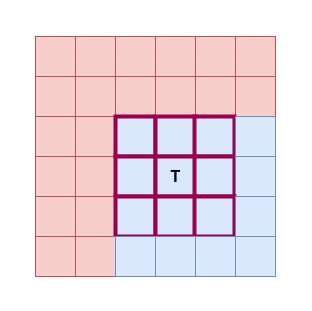
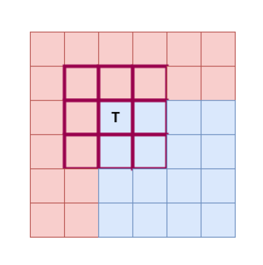
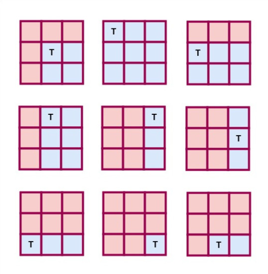
Figure 3: The position of a target pixel in a near-boundary and boundary position for a two-class scenario.

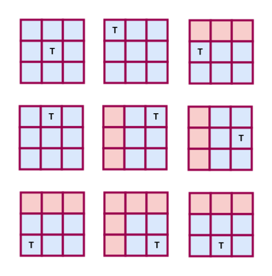
Figure 4: Example of Target-Patch-Orientation of a target pixel lies at the boundary of a class.

Figure 5: Example of Target-Patch-Orientation of a target pixel lies at the near boundary of a class.

II-B Network Architecture

The framework of the HSI classification is shown in Fig 1. It consists of mainly three blocks, namely, band-reduction, feature extraction, and classification. TPO extracts samples from the given dataset as described in Section II-A. The label of each sample is that of the pixel located in the center of the first view among the nine views (discussed in Sec II-A).

II-B1 Band-Reduction

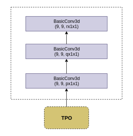
Figure 6: Diagram of the Band Reduction layer in the proposed network.

This block contains three consecutive “BasicConv3d” layers. The designed “BasicConv3d” layer contains 3-D batch-normalization layer and rectified linear unit (ReLU) layer sequentially after 3-D point-wise convolution layer. Parameters of 3-D convolution layer are the input channel, output channel, and the kernel size. In our experiment we have kept input channel$=9$ and output channel$=9$. However, we have empirically adjusted kernel size of three “BasicConv3d” layers which is of the form (X,1,1). Hence, we have used X=p, X=q, and X=r notation in defining kernel size in Fig 6. The aim of choosing such kernel dimension is not to change the spatial size but to reduce the number of bands. Dimension of the input to this layer is $v\times d\times k\times k$ where $v$ represents number of views in the TPO scheme, $d$ represents spectral dimensionality and $k$ is spatial size. We consider $v=9,~{}d=103,$ and $k=5$ to illustrate the network description. The first 3-D convolutional layer (C1) primarily filters the input with dimension $9\times 103\times 5\times 5$ with kernel of size $8\times 1\times 1$, producing a $9\times 96\times 5\times 5$ feature map. In this layer dimension of spectral channels gets reduced from 103 to 96.
As we have used point-wise 3-D convolution, there is no change in the spatial size of the sample. But, the size of the spectral channel is changed based on the value of p which is 8 in this example. The size of the spectral channel in the convolved sample can be computed using the following equation.

$$\left\lfloor\frac{W-K+2P}{S}\right\rfloor+1.$$ (2)

Where $W$ represents the size of the spectral channel, which is $103$ in this case. $K,P$, and $S$ represent kernel size, padding, and stride. For the above example, $K=8$, $P=0$ and $S=1$ holds. Therefore, we are getting 96 channels in the convolved sample. The second layer (C2) combines the features obtained in the C1 layer with nine $16\times 1\times 1$ kernels, resulting in a $9\times 81\times 5\times 5$ feature map. The third layer (C3) combines the features obtained in the C1 layer with nine $32\times 1\times 1$ kernels, resulting in a $9\times 50\times 5\times 5$ feature map. We have a reduced number of bands from 103 to 50 at this point. Now we reshape our data in 3 dimensions by stacking nine views for each 50 spectral information, leading to $450\times 5\times 5$-sized sample. We feed the reshaped output of band-reduction block to feature extraction layer.

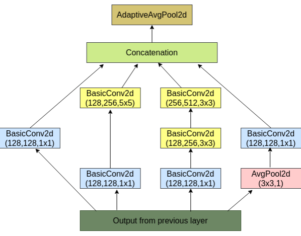
Figure 7: Diagram of the Feature Extraction layer (MS-CNN1) in the proposed network.

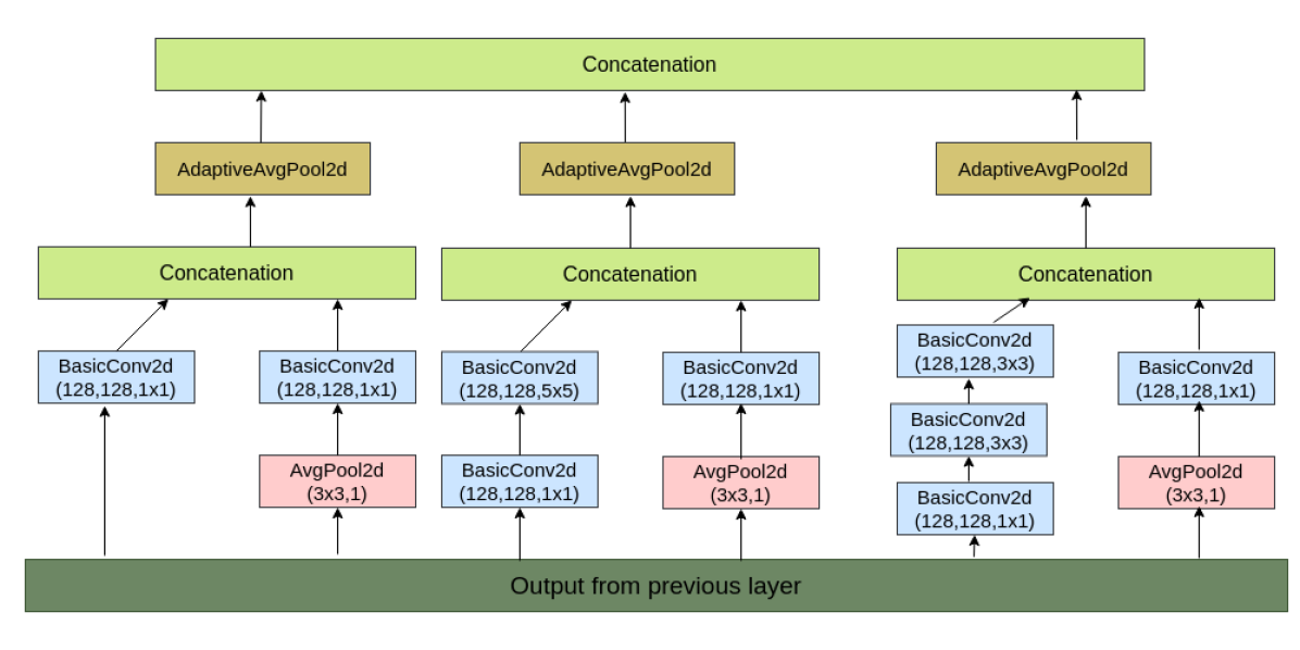
Figure 8: Diagram of the Feature Extraction layer (MS-CNN2) in the proposed network.

II-B2 Feature Extraction

We have taken a tiny patch as an input sample. Our assumption is that a shallow but wider network, i.e., “multi-scale filter bank” extracts more appropriate features from small patches. Hence, we have considered similar to inception-module for feature extraction. We use inception module in two different ways forming two separate networks. Fig 7 and Fig 8 depict feature extraction modules of MS-CNN1 and MS-CNN2 . Each “BasicConv2d” layer in the figures contains a 2-D batch-normalization layer and rectified linear units (ReLU) sequentially after 2-D convolution layer. Parameter of the 2-D convolution layer is the input channel, output channel, and the kernel size. Each rectangular block of “BasicConv2d” in the diagram contains parameters of the 2-D convolution layer. We denote this by $\mathbb{C}_{k_{1}\times k_{1}\times B}$, where $k_{1}$ refers to the kernel size of the convolution layer and $B$ is the number of input channel. On the other hand, each block of “AvgPool2d” depicts the kernel size and the stride value for the average pooling layer in the diagram. We denote this by $\mathbb{P}_{k_{2}\times k_{2}}$, where $k_{2}$ refers to the kernel size of the pooling layer. MS-CNN1 uses a multi-scale filter bank that locally convolves the input sample with four parallel blocks with different filter sizes in convolution layer. Each parallel block consists of either one or many “BasicConv2D” layer and pooling layer. MS-CNN1 has the following details: : $\mathbb{C}_{1\times 1\times B}$ , $\mathbb{C}_{1\times 1\times B}$ followed by $\mathbb{C}_{3\times 3\times B}$ followed by $\mathbb{C}_{3\times 3\times B}$, $\mathbb{C}_{1\times 1\times B}$ followed by $\mathbb{C}_{5\times 5\times B}$ and $\mathbb{P}_{3\times 3}$ followed by $\mathbb{C}_{1\times 1\times B}$. The $3\times 3$ and $5\times 5$ filters are used to exploit local spatial correlations of the input sample while the $1\times 1$ filters are used to address correlations among nine views and their respective spectral information. The outputs of the MS-CNN1 feature extraction layer are combined at concatenation layer to form a joint view-spatio-spectral feature map used as input to the subsequent layers. However, since the size of the feature maps from the four convolutional filters is different from each other, we have padded the input feature with zeros to match the size of the output feature maps of each parallel blocks. For example, we have padded input with 0, 1 and 2 zeros for $1\times 1$ , $3\times 3$ and $5\times 5$ filters, respectively. In MS-CNN1, we have used an adaptive average pooling [41] layer sequentially after the concatenation layer. However, we have split the inception architecture of MS-CNN1 into three small inception layer. Each has two parallel convolutional layers. Each concatenation layer is followed by an adaptive average pooling layer. Finally, we concatenate all the pooled information.

II-B3 Classification

Outputs of feature extraction block are flattened and fed to the fully connected layers whose output channel is the number of class. The fully connected layers is followed by 1-D Batch-Normalization layer and a softmax activation function. In general, the classification layer can be defined as

$$p=softmax(BN(Wa+b))$$ (3)

where $a$ is the input of the fully connected layer, and $W$ and $b$ are the weights and bias of the fully connected layer, respectively. BN($\cdot$) is the 1-D Batch-Normalization layer. $p$ is the $C$-dimensional vector which represents the probability that a sample belongs to the $c^{th}$ class.

II-C Learning the Proposed Network

We have trained the proposed networks by minimizing cross-entropy loss function. Let $Y=\{y_{i}\}_{i=1}^{b}$ represents the ground-truth for the training samples present in a batch $b$. $P=\{p_{ic}\}_{i=1}^{b}$ denotes the conditional probability distribution of the model. The model predicts that $i^{th}$ training sample belongs to the $c^{th}$ class with probability $p_{ic}$. The cross-entropy loss function $\mathbb{L}_{cross-entropy}$ is given by

$$\mathbb{L}_{cross-entropy}=-\sum_{i=1}^{b}\sum_{c=1}^{C}y_{i}[c]\log{p_{ic}}$$ (4)

In our dataset, the ground truth is represented as one-hot encoded vector. Each $y_{i}$ is a $C$ dimensional vector and $C$ represents the number of classes. If the class label of the $i^{th}$ sample is $c$ then,

$$\begin{cases}y_{i}[j]=1&\text{if}~{}j=c\\ y_{i}[j]=0&\text{, Otherwise}\end{cases}$$

To train the model, Adam optimizer with a batch size of 512 samples is used with a weight decay of 0.0001 . We initially set a base learning rate as 0.0001. All the layers are initialized from a uniform distribution.

III Experimental Results

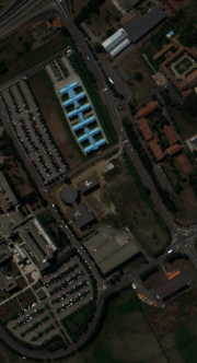
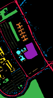
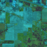
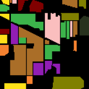
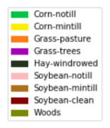
Figure 9: University of Pavia dataset. Three-band color composite image is given on left, ground truth is given in the middle, and color code used in ground-truth is shown on the right.

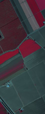
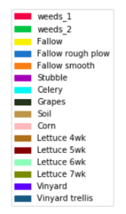
Figure 10: Indian Pines dataset. Three-band color composite image is given on left, ground truth is given in the middle, and color code used in ground-truth is shown on the right.

Figure 11: Salinas dataset. Three-band color composite image is given on left, ground truth is given in the middle, and color code used in ground-truth is shown on the right.

TABLE I: A brief description on HSI Datasets

	U. Pavia	Indian Pines	Salinas
Sensor	ROSIS	AVIRIS	AVIRIS
Place	Pavia, Northern Italy	Northwestern Indiana	Salinas valey california
wavelength range	0.43-0.86 $\mu m$	0.4-2.5 $\mu m$	0.4-2.5 $\mu m$
Spatial Resolution	1.3 m	20 m	3.7 m
No of bands	103	220	224
No. of Classes	9	16	16
Image size	$610\times 340$	$145\times 145$	$512\times 217$

III-A Datasets

The performance of HSI classification is observed by experimenting with three popular datasets: the Pavia University scene (U.P) (Fig-11), the Indian Pines (I.P) (Fig-11), and the Salinas (S) dataset (11). Table I contains a brief description about the datasets. We have discarded $20$ water absorption bands in Indian Pines. Also, we have rejected some classes in Indian Pines dataset which has less than 400 samples. We have selected 200 labeled pixels from each class to prepare a training set for each of the three HSI datasets. The rest of the labeled samples constitute the test set. As different spectral channels range differently, we normalize them to the range [0, 1] using the function $\mathbb{F}(\cdot)$ defined in Eq. 5, where $x$ denotes the pixel value of a given spectral channel and $\mu$ and $\sigma$ provide mean and standard deviation of the complete dataset.

$$\mathbb{F}(x)=\frac{x-\mu}{\sigma}$$ (5)

III-B Quantitative Metrics

We evaluate the performance of the proposed architecture quantitatively in terms of the following metrics.

III-B1 Overall Accuracy(OA)

Overall Accuracy is computed using the following formulae in the test samples where $C=$number of classes, considered for a given HSI dataset:

$$OA=\frac{\sum_{c_{i}\in C}\text{\#Correctly classified samples in class~{}}c_{i}}{\sum_{c_{i}\in C}\text{\#samples in class~{}}c_{i}}$$ (6)

III-B2 Average Accuracy (AA)

Average Accuracy is computed using the following formulae in the test samples where $C=$number of classes, considered for a given HSI dataset:

$$AA=\frac{1}{C}\sum_{c_{i}\in C}\frac{\text{\#correctly classified samples in class}~{}c_{i}}{\text{\#samples in class}~{}c_{i}}$$ (7)

III-B3 $\kappa$-score

The $\kappa$-score [18] is a statistical measure about the agreement between two classifiers. Each classifier classifies N samples into C mutually exclusive classes. $\kappa$-score is given by the following equation:

$$\kappa=\frac{p_{o}-p_{e}}{1-p_{e}}$$ (8)

where $p_{o}$ is the relative observed agreement between classifiers, and $p_{e}$ is the hypothetical probability of chance agreement. $\kappa=1$ indicates complete agreement between two classifiers, while $\kappa\leq 0$ refers no agreement at all.

III-C Implementation Platform

The network is implemented in pytorch, a popular deep learning library, written in python. We have trained our models on a machine with GeForce GTX 1080 Ti GPU.

III-D Comparison with Other Methods

The key features of our proposed methods are 1) use of both spectral and spatial features, 2) band-reduction using several consecutive 3-D CNNs and 3) feature extraction with a multi-scale convolutional network. We have chosen six state of the art methods namely,: 1) CNN-PPF [30], 2) DR-CNN [31], 3) 2S-Fusion [32], 4) BASS [34], 5) DPP-ML [33], and 6) S-CNN+SVM [35]. Every comparable method exploits both spectral and spatial features. CNN-PPF uses a pixel pair strategy to increase the number of training samples and feeds them into a deep network having 1-D convolutional layers. DR-CNN exploits diverse region-based 2-D patches from the image to produce more discriminative features. On the contrary, 2S-Fusion processes spatial and spectral information separately and fuses them using adaptive class-specific weights. However, BASSNET extracts band specific spatial-spectral features. In DPP-ML, convolutional neural networks with multiscale convolution are used to extract deep multiscale features from the HSI. SVM-based methods are common in traditional hyperspectral image classification. In S-CNN+SVM, the Siamese convolutional neural network extracts spectral-spatial features of HSI and feeds them to a SVM classifier. In general, the performance of deep learning-based algorithms supersedes traditional techniques (e.g, k-NN, SVM, ELM). We have compared the performance of the proposed techniques with the best results reported for each of these state of the art techniques. In S-CNN+SVM and 2S-Fusion, performance on the salinas dataset is not reported. To maintain consistency in the results, we ran our algorithm with the classes and the number of samples for each class used in 2S-Fusion, DR-CNN, DPP-ML for Indian Pines.

TABLE II: Class-specific Accuracy(%) and OA of comparable techniques for the University of Pavia dataset

Class	Training samples	CNN -PPF	BASS	S-CNN +SVM	2S -Fusion	DR -CNN	DPP -ML	MS- CNN1	MS- CNN2
Asphalt	200	97.42	97.71	100	97.47	98.43	99.38	99.78	100
Meadows	200	95.76	97.93	98.12	99.92	99.45	99.59	99.88	99.99
Gravel	200	94.05	94.95	99.12	83.80	99.14	97.33	99.21	100
Trees	200	97.52	97.80	99.40	98.98	99.50	99.31	99.41	99.93
Painted metal sheets	200	100	100	99.18	100	100	100	100	100
Bare Soil	200	99.13	96.60	99.10	97.75	100	99.99	99.75	100
Bitumen	200	96.19	98.14	98.50	77.44	99.70	99.85	100	100
Self-Blocking Bricks	200	93.62	95.46	99.91	96.65	99.55	99.02	99.77	100
Shadows	200	99.60	100	100	99.65	100	100	100	100
OA		96.48	99.68	97.50	99.56	99.46	99.72	99.78	99.99

TABLE III: Class-specific Accuracy(%) and OA of comparable techniques for the Indian Pines dataset. Training and testing is restricted to 9 classes.

Number of training samples per class=200
Class	CNN- PPF	BASS	S-CNN +SVM	MS- CNN1	MS- CNN2
Corn-notil	92.99	96.09	98.25	100	100
Corn-mintil	96.66	98.25	99.64	99.92	99.75
Grass-pasture	95.58	100	97.10	100	99.68
Grass-tree	100	99.24	99.86	99.73	99.82
Hay-windrowed	100	100	100	100	100
Soybean-notil	96.24	94.82	98.87	100	100
Soybean-mintil	87.80	94.41	98.57	99.74	100
Soybean-clean	98.98	97.46	100	100	100
Woods	99.81	99.90	100	100	99.72
OA	94.34	96.77	99.04	99.89	99.84

TABLE IV: Class-specific Accuracy(%) and OA of comparable techniques for the Indian Pines dataset. DR-CNN and DPP-ML consider 8 classes and 2S-Fusion includes 16 classes for the experiment.

Class	Training samples	DR -CNN	DPP -ML	MS- CNN1	MS- CNN2	Training samples	2S- Fusion	MS- CNN1	MS- CNN2
Alfalfa	-	-	-	-	-	33	100	100	100
Corn-notill	200	98.20	99.03	100	100	861	95.35	100	100
Corn-mintill	200	99.79	99.74	99.51	99.67	501	98.75	100	100
Corn	-	-	-	-	-	141	100	100	100
Grass-pasture	200	100	100	100	100	299	100	100	100
Grass-trees	-	-	-	-	-	449	99.32	100	100
Grass-pasture-mowed	-	-	-	-	-	9	100	100	100
Hay-windrowed	200	100	100	98.84	98.85	294	100	100	100
Oats	-	-	-	-	-	12	100	100	100
Soybean-notill	200	99.78	99.61	100	100	580	100	100	100
Soybean-mintill	200	96.69	97.80	100	99.91	1480	98.03	100	100
Soybean-clean	200	99.86	100	100	100	369	100	100	100
Wheat	-	-	-	-	-	127	97.87	100	100
Woods	200	99.99	100	100	100	777	99.62	100	100
Buildings-Grass-Trees-Drives	-	-	-	-	-	228	98.53	100	100
Stone-Steel-Towers	-	-	-	-	-	57	100	100	100
OA		98.54	99.08	99.54	99.55		98.65	100	100

TABLE V: Class-specific Accuracy(%) and OA of comparable techniques for the Salinas dataset

Class	Training samples	CNN -PPF	BASS	DR -CNN	DPP -ML	MS- CNN1	MS- CNN2
Brocoli-green-weeds-1	200	100	100	100	100	100	100
Brocoli-green-weeds-2	200	99.88	99.97	100	100	100	100
Fallow	200	99.60	100	99.98	100	100	99.72
Fallow-rough-plow	200	99.49	99.66	99.89	99.25	100	100
Fallow-smooth	200	98.34	99.59	99.83	99.44	99.84	99.88
Stubble	200	99.97	100	100	100	100	100
Celery	200	100	99.91	99.96	99.87	100	100
Grapes-untrained	200	88.68	90.11	94.14	95.36	94.30	98.17
Soil-vinyard-develop	200	98.33	99.73	99.99	100	99.75	100
Corn-senesced-green-weeds	200	98.60	97.46	99.20	98.85	94.02	99.35
Lettuce-romaine-4wk	200	99.54	99.08	99.99	99.77	100	100
Lettuce-romaine-5wk	200	100	100	100	100	100	100
Lettuce-romaine-6wk	200	99.44	99.44	100	99.86	100	100
Lettuce-romaine-7wk	200	98.96	100	100	99.77	100	100
Vinyard-untrained	200	83.53	83.94	95.52	90.50	95.08	94.03
Vinyard-vertical-trellis	200	99.31	99.38	99.72	98.94	100	100
OA		94.80	95.36	98.33	97.51	97.98	98.72

III-E Results and Discussion

The performance of the proposed MS-CNN1 and MS-CNN2 on test-samples are compared with the aforementioned deep learning-based classifiers in Tables II, III, IV and V. We have considered the size of spatial window ($k$) for generating a patch as $7$ to evaluate the performance of our algorithms. For Indian-Pines, DR-CNN and DPP-ML used 8 classes, 2S-Fusion used 16 classes and other comparable methods used 9 classes for their experiment. To compare our method we have chosen the same number of classes and training samples of each class as mentioned in the respective papers. Table III and Table IV together indicate that MS-CNN1 and MS-CNN2 provides comparable results and supersedes the other methods. However, MS-CNN2 produces better results compared to MS-CNN1 in University of Pavia and Salinas datasets as shown in Table II and Table V respectively. The results signify that the arrangements of multi-scale convolutions in MS-CNN2 is able to extract more useful features for the classification compared to MS-CNN1.

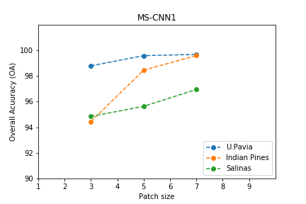
(a)

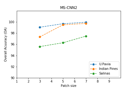
(b)

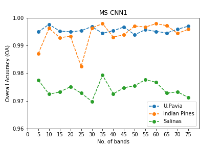
(c)

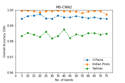
(d)

Figure 12: Variation of test accuracy on the three HSI datasets (a)-(b) with varying patch size, (c)-(d) with reduced number of spectral channels.

We have shown thematic maps generating from the classification of three HSI scenes using our networks in Figure 13. In order to check the consistency of our network, we repeat experiments 10 times with different training sets. Table VI shows the mean and standard deviation of OA over these 10 experiments for each data set.

TABLE VI: Mean and standard deviation of 10 Independent Experiments

Datasets		U.P		I.P		S
MS-CNN		1	2	1	2	1	2
OA	Mean	99.76	99.90	99.67	99.65	98.10	98.65
	Std-dev	0.24	0.06	0.14	0.17	0.37	0.28
AA	Mean	99.80	99.94	99.82	99.78	97.87	98.49
	Std-dev	0.20	0.06	0.07	0.11	0.42	0.30
$\kappa$	Mean	99.44	99.86	99.61	99.58	99.29	99.44
	Std-dev	0.32	0.08	0.17	0.20	0.18	0.14

(a)

(b)

(c)

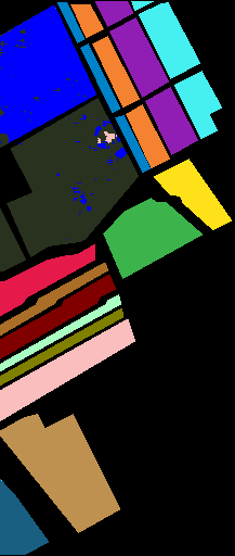
(d)

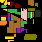
(e)

(f)

Figure 13: Thematic maps resulting from classification using $7\times 7$-patch by MS-CNN1 and MS-CNN2 respectively for (a)-(b) University of Pavia dataset, (c)-(d) Salinas data set, and (e)-(f) Indian Pines dataset. Color code is similar to its ground truths.

TABLE VII: Overall Accuracy (OA) for varying patch size

Patch size	MS-CNN1			MS-CNN2
	U.P	I.P	S	U.P	I.P	S
$3\times 3$	98.78	94.44	94.84	99.05	97.32	95.59
$5\times 5$	99.57	98.44	95.62	99.67	99.47	96.27
$7\times 7$	99.67	99.58	96.94	99.94	99.73	97.46

III-F Comparison of Different Hyper-parameter Settings

There are two hyper-parameters which have a direct effect on the accuracy of classification task: 1) Spatial size of input image, and the 2) Number of spectral channels obtained from the band reduction block. Figures 12(a) and 12(b) depicts test accuracies on 3 HSI datasets for different choices of input patch size on the same randomly selected training sample. We observe that with increasing patch size accuracies in University of Pavia, Indian Pines and Salinas increase in both the networks. Table VIII shows the adjusted $(p,q,r)$ (refer to Section II-B1) parameters used for 3 HSI datasets. We vary the value of $r$ to get a different number of bands and observe its impact on classification accuracy. We did not observe any monotonically increasing or decreasing behavior in overall classification accuracy for changing the number of bands with varying value of $r$. Figures 12(c) and 12(d) depicts the change in overall accuracy (OA) for varying $r$. They suggest that ($r_{\text{MS-CNN2}}=35$ and $r_{\text{MS-CNN1}}=35$), ($r_{\text{MS-CNN2}}=20$ and $r_{\text{MS-CNN1}}=10$) ,($r_{\text{MS-CNN2}}=40$ and $r_{\text{MS-CNN1}}=35$) are suitable for University of Pavia, Indian Pines, Salinas, respectively.

TABLE VIII: Parameters in Band Reduction Block

	U.P	I.P	S
p	8	32	32
q	16	57	61
r	32	64	64

III-G Classification performance with decreasing number of training samples

In this section, the influence of decreasing the number of samples on the classification accuracy has been studied on the University of Pavia, Indian Pines, and Salinas datasets. We present the experimental results with the setup as mentioned above with $7\times 7$ spatial resolution. Here, each class selects a fixed number $(t)$ of samples per class from the labeled pixels. To showcase the effect of decreasing number of training samples on the classification accuracy, we have chosen several values of $t$, e.g., 150, 100, and 50. Our proposed architecture still performs better than most of the comparable methods with 150 training samples per class. Table IX reassures that network architecture for feature extraction in MS-CNN2 brings more useful feature for University of Pavia, India Pines, and Salinas datasets even with a small number of training samples compared to MS-CNN1.

TABLE IX: Performance measures on the three datasets with decreasing number of training samples. metrics are the average of 10 independent experiments.

#samples		150		100		50
MS-CNN		1	2	1	2	1	2
U.P	OA std. dev.	99.58 (0.22)	99.93 (0.05)	99.16 (0.62)	99.75 (0.13)	98.25 (1.15)	98.98 (0.62)
	AA std. dev.	99.76 (0.08)	99.92 (0.06)	98.88 (0.82)	99.67 (0.17)	97.68 (1.50)	98.65 (0.82)
	$\kappa$ std. dev.	99.44 (0.30)	99.91 (0.07)	99.45 (0.31)	99.82 (0.07)	98.54 (0.74)	99.17 (0.39)
I.P	OA std. dev.	99.44 (0.12)	99.47 (0.18)	98.72 (0.46)	98.88 (0.35)	94.12 (1.32)	95.88 (1.02)
	AA std. dev.	99.33 (0.15)	99.38 (0.22)	98.49 (0.55)	98.67 (0.42)	93.10 (1.54)	95.22 (1.25)
	$\kappa$ std. dev.	99.59 (0.20)	99.60 (0.24)	99.15 (0.30)	99..23 (0.19)	96.21 (0.77)	97.18 (0.50)
S	OA std. dev.	97.39 (0.24)	97.51 (0.39)	96.48 (0.44)	96.92 (0.39)	95.81 (0.29)	96.28 (0.39)
	AA std. dev.	99.06 (0.11)	99.21 (0.09)	98.60 (0.12)	98.68 (0.20)	98.26 (0.33)	98.48 (0.24)
	$\kappa$ std. dev.	97.08 (0.27)	97.22 (0.44)	96.08 (0.49)	96.56 (0.44)	95.33 (0.33)	95.86 (0.43)

III-H Ablation study of the TPO strategy

In order to judge how the TPO strategy, as described in Section II-A affects the performance of the classifier, we compare the classification results using a single view where the position of the target pixel is the center of the given window. Table X supports the fact that the TPO strategy has a direct effect on the classification accuracies. We observe that OA increases by 6.09%, 13.18% 1.37% in MS-CNN1 model and 9.99%, 14.55% 2.08% in MS-CNN2 model for classification of University of Pavia, Indian Pines, Salinas, respectively. In brief, the TPO-scheme improves results in every dataset for both the models. This suggests consistent behavior and a positive impact of TPO-strategy on each model for all three datasets. Again, we observe MS-CNN2 provides better results compared to MS-CNN1. We have highlighted misclassified pixels with white color code in Figure 17 and Figure 16(f).

III-H1 Description of metrics for quantitative analysis

We have proposed a few metrics to analyze the impact of the TPO scheme in the models. $\tau$ in Equation 9 reveals the percentage of misclassified pixels along the boundary (B) or non-boundary (NB) regions.

$$\tau=\frac{\sum_{c_{i}\in C}\text{\#samples misclassified in B (NB)}}{\sum_{c_{i}\in C}\text{\#samples in B (NB)}}\times 100$$ (9)

We have proposed $\nu(a\rightarrow b)$ in Equation 10 to understand the impact of including TPO scheme in the proposed models. $tc(\cdot)$ determines truely classified pixels. $mc(\cdot)$ determines misclassified pixels. $a,b\in\{Yes,No\}$. The condition (TPO=a) indicates whether TPO scheme is considered.

Similarly, We have proposed $\mu(a\rightarrow b)$ in Equation 11 to understand the impact of switching models. $\mathcal{M}$ denotes deep model whose values can be $a$ or $b$. $a,b\in\{\text{MS-CNN1},\text{MS-CNN2}\}$

III-H2 Impact of TPO scheme on each model

Table XII clearly shows that the misclassification rate reduces along the boundary and non-boundary regions with the inclusion of the TPO scheme.

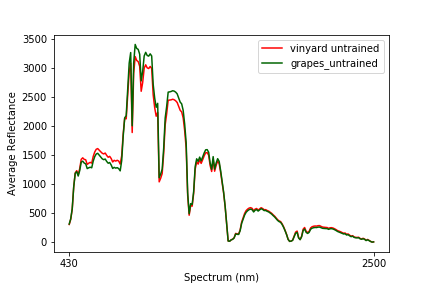
Figure 14: Average reflectance spectrum of pixels whose prediction is similar to ground truth by each model with and without the TPO scheme,

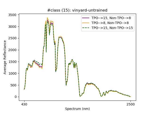
(a)

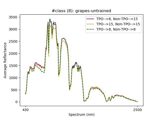
(b)

Figure 15: Average reflectance spectrum of selected samples based on three conditions. TPO$\rightarrow$‘X’ and Non-TPO$\rightarrow$‘Y’ represents prediction for the sample by the two models with the TPO scheme is ‘X’ and non-TPO scheme is ‘Y’. Legends show the three conditions.

A critical challenge in hyper-spectral imaging is that some pixels which belong to the same land cover class may have different spectral signatures due to complex light scattering mechanism. Therefore, an approach that is capable of making generalized features for the case, as mentioned above, can offer better classification accuracies. We discuss the impact of the TPO approach on the above issue in Salinas dataset. We found that the class=‘vinyard-untrained’ has highest percentage of misclassification by every model irrespective of TPO scheme. Also, it is identified that most of them are misclassified as ’grapes-untrained’. For ‘vinyard-untrained’ and ‘grapes-untrained’ in Salinas, we calculate the average of reflectance of selected samples for each spectral band belonging to the respective class and name it Average Reflectance Spectrum (ARS). In Figure 14, we have shown ARS for ‘vinyard-untrained’ and ‘grapes-untrained’ in Salinas dataset . As shown in this figure, two of them have very similar reflectance spectrum. In Figure 15, we have selected samples for computing ARS on the basis of three conditions: i) samples that are correctly predicted by each model with TPO and non-TPO scheme, ii) samples are correctly predicted by each model with the TPO scheme but misclassified by each model with non-TPO scheme, and iii) samples that are misclassified by each model with TPO and non-TPO scheme. The first condition incorporates most of the samples of the respective class. Figure 15 clearly reveals that the class has different reflectance spectrum within itself. Additionally, it shows that the TPO scheme is able to predict correctly a fraction of class members whose reflectance spectrum is different from the majority of the class members. Equation 12 quantitatively analyze the improvement in classification of pixels due to incorporation of the TPO approach. We have tabulated values of Equation 12 in Table XI. It clearly states that TPO-scheme has positive effect on the class which has different spectral signature.

Additionally, Table XIII reveals that the percentage of boundary pixels that are correctly classified with TPO inclusion is more compared to the non-boundary region in all three datasets. However, we have observed that a tiny fraction which is correctly classified without including TPO-scheme gets misclassified with TPO-scheme.

III-H3 Impact of models on TPO scheme

Table XIV considers two cases. Case-1 denotes the number of pixels that are misclassified by MS-CNN1 but correctly classified by MS-CNN2. Case-2 indicates the number of pixels that are misclassified by MS-CNN2 but correctly classified by MS-CNN1. When case-1 supersedes case-2, we may conclude MS-CNN2 is a better performer compared to MS-CNN1. Table XIV suggests an inconsistent behavior without the TPO scheme. It shows case-1 supersedes case-2 for Indian Pines in the non-boundary region and salinas in the boundary region. However, with TPO-scheme, case-1 always supersedes case-2 for all three datasets in both boundary and non-boundary regions. Our observation suggests that MS-CNN2 performs better with the TPO-scheme. However, MS-CNN1 has no generalized behavior for all three datasets in either including the TPO-scheme or excluding it.

IV Conclusion

In this paper, a hybrid of 3-D and 2-D CNN-based network architecture is proposed for HSI classification. We also propose a strategy (namely, target-pixel orientation (TPO)) to incorporate spatial and spectral information of HSI. In general, classification accuracy degrades due to a class having different spectral signatures in HSI. With incorporation of spectral and spatial information together, classification accuracy can be improved. But, mis-classification at the boundary region still exists as the spatial neighborhood is different in a boundary region compared to a non-boundary region. Our approach attempts to take care of this limitation by using the orientation of the Target-pixel-view. Our architectural design of neural network exploits point-wise 3-D convolutions for band reduction whereas we adopt multi-scale 2-D inception like architecture for feature extraction. We have tested the granular arrangement of multi-scale convolutions in inception like architecture in MS-CNN2. We find MS-CNN2 provides better results compared to MS-CNN1. The experimental results with real hyperspectral images demonstrates the positive impact of including TPO strategy. Also, the proposed work improves the performance of the classification accuracy compared to the state of the art methods even with a smaller number of training samples (For example, 150 samples per class). All the experimental results suggest that the arrangement of multi-scale convolutions in MS-CNN2 provides more useful features compared to MS-CNN1. Experiments show that TPO-scheme is working better in MS-CNN2.

(a) without TPO

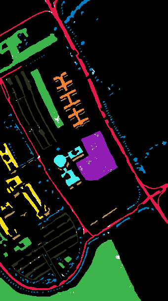
(b) with TPO

(c) without TPO

(d) with TPO

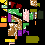
(e) without TPO

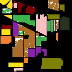
(f) with TPO

Figure 17: Thematic maps resulting from classification using $3\times 3$-patch by MS-CNN2 for (a)-(b) Salinas dataset , (c)-(d) University of Pavia dataset, and (e)-(f) Indian Pines dataset respectively. Color code is similar to its ground truths. White color code is used to show misclassified pixels.

Figure 16: Thematic maps resulting from classification using $3\times 3$-patch by MS-CNN1 for (a)-(b) University of Pavia dataset, (c)-(d) Salinas dataset and (c)-(d) Indian Pines dataset respectively. Color code is similar to its ground truths. White color code is used to show misclassified pixels.

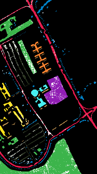
(g) without TPO

(h) with TPO

(i) without TPO

(j) with TPO

(k) without TPO

(l) with TPO

TABLE X: Impact of TPO-strategy on the classification considering $3\times 3$ spatial size

TPO	metric	U.P	I.P	S
MS-CNN1
No	OA	92.69	81.26	93.47
	AA	92.32	88.40	97.14
	$\kappa$	90.24	77.82	92.69
Yes	OA	98.78	94.44	94.84
	AA	98.60	96.92	97.73
	$\kappa$	98.36	93.36	94.22
MS-CNN2
No	OA	89.06	82.27	93.51
	AA	91.14	88.73	97.26
	$\kappa$	85.50	78.97	92.73
Yes	OA	99.05	97.32	95.59
	AA	98.94	98.40	98.35
	$\kappa$	98.72	96.79	95.07

TABLE XI: Percentage of pixels misclassified ($\alpha(X|Y)$) by both MS-CNN1 and MS-CNN2

#True Class	TPO	boundary	non-bounday
	misclassified as ‘grapes-untrained’ (X)
‘vinyard- untrained (Y)’	Yes	14.48	8.06
	No	19.54	13.27
	misclassified as ‘vinyard-untrained’ (X)
grapes- untrained (Y)	Yes	9.20	7.02
	No	9.61	7.55

TABLE XII: Total misclassification (in %) of pixels ($\tau$) in boundary and non-boundary region. Bold fond is used to highlight lower misclassification.

Dataset	Models	MS-CNN1		MS-CNN2
	TPO	No	Yes	No	Yes
U. P	Boundary	8.03	1.75	12.39	1.42
	Non-boundary	6.42	0.84	9.42	0.62
I.P	Boundary	18.60	8.10	19.27	8.14
	Non-boundary	13.87	3.22	12.54	1.12
S	Boundary	6.69	5.72	6.18	4.26
	Non-boundary	6.09	4.80	6.12	4.15

TABLE XIII: Impact of TPO scheme (metric $\nu(a\rightarrow b)$) for the improvement of classification in boundary and non-boundary regions. N abbreviates No and Y abbreviates Yes.

Dataset Models MS-CNN1 MS-CNN2 $\nu(N\rightarrow Y)$ $\nu(Y\rightarrow N)$ $\nu(N\rightarrow Y)$ $\nu(Y\rightarrow N)$ U. P Boundary 7.28 0.97 11.70 0.74 Non-boundary 5.98 0.41 9.19 0.39 I.P Boundary 14.13 3.63 15.73 1.60 Non-boundary 11.35 0.70 11.82 0.39 S Boundary 3.23 2.26 3.67 1.75 Non-boundary 2.98 1.70 3.61 1.64

TABLE XIV: Impact of models (metric $\mu$) on the improvement of classification in boundary and non-boundary region.
$a=\text{\emph{MS-CNN1}}$ and $b=\text{\emph{MS-CNN2}}$

Dataset TPO No Yes Models $\mu(a\rightarrow b)$ $\mu(b\rightarrow a)$ $\mu(a\rightarrow b)$ $\mu(b\rightarrow a)$ U. P Boundary 4.77 9.13 1.05 0.72 Non-boundary 4.00 7.00 0.61 0.39 I.P Boundary 7.84 8.52 4.72 1.77 Non-boundary 7.28 5.96 2.64 0.54 S Boundary 2.63 2.12 2.85 1.39 Non-boundary 2.41 2.44 2.02 1.36

Jayasree Saha received M.Tech degree from University of Calcutta in 2014. She is currently pursuing the Ph.D degree with the Department of Computer Science and Engineering, Indian Institute of Technology (IIT), Kharagpur, India. Her research interest includes computer vision, remote sensing and deep learning.

Yuvraj Khanna is currently pursuing the Dual degree with the Department of Electronics and Electrical communications and Engineering, Indian Institute of Technology (IIT), Kharagpur, India. His research interest includes remote sensing and deep learning

Jayanta Mukherjee received his B.Tech., M.Tech., and Ph.D. degrees in Electronics and Electrical Communication Engineering from the Indian Institute of Technology (IIT), Kharagpur in 1985, 1987, and 1990, respectively. He is currently a Professor with the Department of Computer Science and Engineering, Indian Institute of Technology (IIT), Kharagpur, India. His research interests are in image processing, pattern recognition, computer graphics, multimedia systems and medical informatics. He has published about 250 research papers in journals and conference proceedings in these areas. He received the Young Scientist Award from the Indian National Science Academy in 1992. Dr. Mukherjee is a Senior Member of the IEEE. He is a fellow of the Indian National Academy of Engineering (INAE).

References

- [1] G. Hughes, “On the mean accuracy of statistical pattern recognizers,” in IEEE Transactions on Information Theory, vol. 14, no. 1, pp. 55-63, 1968.
- [2] A. Villa, J. A. Benediktsson, J. Chanussot and C. Jutten, “Hyperspectral Image Classification With Independent Component Discriminant Analysis,” in IEEE Transactions on Geoscience and Remote Sensing, vol. 49, no. 12, pp. 4865-4876, Dec. 2011.
- [3] G. Licciardi, P. R. Marpu, J. Chanussot and J. A. Benediktsson, “Linear Versus Nonlinear PCA for the Classification of Hyperspectral Data Based on the Extended Morphological Profiles,” in IEEE Geoscience and Remote Sensing Letters, vol. 9, no. 3, pp. 447-451, 2012.
- [4] J. Li et al., “Multiple Feature Learning for Hyperspectral Image Classification,” in IEEE Transactions on Geoscience and Remote Sensing, vol. 53, no. 3, pp. 1592-1606, 2015.
- [5] G. Camps-Valls and L. Bruzzone, “Kernel-based methods for hyperspectral image classification,” in IEEE Transactions on Geoscience and Remote Sensing, vol. 43, no. 6, pp. 1351-1362, 2005.
- [6] W. Li, S. Prasad, J. E. Fowler and L. M. Bruce, “Locality-Preserving Dimensionality Reduction and Classification for Hyperspectral Image Analysis,” in IEEE Transactions on Geoscience and Remote Sensing, vol. 50, no. 4, pp. 1185-1198, 2012.
- [7] X. Wang, Y. Kong, Y. Gao and Y. Cheng, “Dimensionality Reduction for Hyperspectral Data Based on Pairwise Constraint Discriminative Analysis and Nonnegative Sparse Divergence,” in IEEE Journal of Selected Topics in Applied Earth Observations and Remote Sensing, vol. 10, no. 4, pp. 1552-1562, 2017.
- [8] S. Chen and D. Zhang, “Semisupervised Dimensionality Reduction With Pairwise Constraints for Hyperspectral Image Classification,” in IEEE Geoscience and Remote Sensing Letters, vol. 8, no. 2, pp. 369-373, 2011.
- [9] W. Zhao and S. Du, “Spectral–Spatial Feature Extraction for Hyperspectral Image Classification: A Dimension Reduction and Deep Learning Approach,” in IEEE Transactions on Geoscience and Remote Sensing, vol. 54, no. 8, pp. 4544-4554, 2016.
- [10] F. A. Mianji and Y. Zhang, “Robust Hyperspectral Classification Using Relevance Vector Machine,” in IEEE Transactions on Geoscience and Remote Sensing, vol. 49, no. 6, pp. 2100-2112, 2011.
- [11] A. Samat, P. Du, S. Liu, J. Li and L. Cheng, “ : Ensemble Extreme Learning Machines for Hyperspectral Image Classification,” in IEEE Journal of Selected Topics in Applied Earth Observations and Remote Sensing, vol. 7, no. 4, pp. 1060-1069, 2014.
- [12] W. Li, C. Chen, H. Su and Q. Du, “Local Binary Patterns and Extreme Learning Machine for Hyperspectral Imagery Classification,” in IEEE Transactions on Geoscience and Remote Sensing, vol. 53, no. 7, pp. 3681-3693, 2015.
- [13] T. Lu, S. Li, L. Fang, L. Bruzzone and J. A. Benediktsson, “Set-to-Set Distance-Based Spectral–Spatial Classification of Hyperspectral Images,” in IEEE Transactions on Geoscience and Remote Sensing, vol. 54, no. 12, pp. 7122-7134, 2016.
- [14] Guang-Bin Huang, Qin-Yu Zhu, Chee-Kheong Siew, “Extreme learning machine: Theory and applications,” Neurocomputing, vol 70, Issues 1-3, pp. 489-501, 2006.
- [15] Jie Gui, Zhenan Sun, Wei Jia, Rongxiang Hu, Yingke Lei, Shuiwang Ji, “Discriminant sparse neighborhood preserving embedding for face recognition,” Pattern Recognition, vol. 45, Issue 8, pp 2884-2893, 2012.
- [16] D. Lunga, S. Prasad, M. M. Crawford and O. Ersoy, “Manifold-Learning-Based Feature Extraction for Classification of Hyperspectral Data: A Review of Advances in Manifold Learning,” in IEEE Signal Processing Magazine, vol. 31, no. 1, pp. 55-66, 2014.
- [17] Christian Szegedy, Sergey Ioffe and Vincent Vanhoucke, “Inception-v4, Inception-ResNet and the Impact of Residual Connections on Learning,” in CoRR, vol. abs/1602.07261, arXiv, 2016.
- [18] Cohen, J. A Coefficient of Agreement for Nominal Scales. Educational and Psychological Measurement, vol. 20, no. 1, pp. 37-46. 1960.
- [19] S. Jia, X. Zhang and Q. Li, “Spectral–Spatial Hyperspectral Image Classification UsingRegularized Low-Rank Representation and Sparse Representation-Based Graph Cuts,” in IEEE Journal of Selected Topics in Applied Earth Observations and Remote Sensing, vol. 8, no. 6, pp. 2473-2484, 2015.
- [20] H. Zhang, Y. Li, Y. Jiang, P. Wang, Q. Shen and C. Shen, “Hyperspectral Classification Based on Lightweight 3-D-CNN With Transfer Learning,” in IEEE Transactions on Geoscience and Remote Sensing, vol. 57, no. 8, pp. 5813-5828, 2019.
- [21] S. K. Roy, G. Krishna, S. R. Dubey and B. B. Chaudhuri, “HybridSN: Exploring 3-D-2-D CNN Feature Hierarchy for Hyperspectral Image Classification,” in IEEE Geoscience and Remote Sensing Letters, pp. 1-5, 2019.
- [22] Y. Chen, X. Zhao and X. Jia, “Spectral–Spatial Classification of Hyperspectral Data Based on Deep Belief Network,” in IEEE Journal of Selected Topics in Applied Earth Observations and Remote Sensing, vol. 8, no. 6, pp. 2381-2392, June 2015.
- [23] T. Li, J. Zhang and Y. Zhang, “Classification of hyperspectral image based on deep belief networks,” IEEE International Conference on Image Processing (ICIP), pp. 5132-5136, 2014.
- [24] P. Zhong, Z. Gong, S. Li and C. Schönlieb, “Learning to Diversify Deep Belief Networks for Hyperspectral Image Classification,” in IEEE Transactions on Geoscience and Remote Sensing, vol. 55, no. 6, pp. 3516-3530, 2017.
- [25] P. Zhong, Zhiqiang Gong and C. Schönlieb, “A DBN-crf for spectral-spatial classification of hyperspectral data,” 23rd International Conference on Pattern Recognition (ICPR), pp. 1219-1224, 2016.
- [26] J. Feng, L. Liu, X. Zhang, R. Wang and H. Liu, “Hyperspectral image classification based on stacked marginal discriminative autoencoder,” 2017 IEEE International Geoscience and Remote Sensing Symposium (IGARSS), Fort Worth, TX, 2017, pp. 3668-3671.
- [27] J. E. Ball and P. Wei, “Deep Learning Hyperspectral Image Classification using Multiple Class-Based Denoising Autoencoders, Mixed Pixel Training Augmentation, and Morphological Operations,” IEEE International Geoscience and Remote Sensing Symposium (IGARSS), pp. 6903-6906, 2018.
- [28] J. Feng, L. Liu, X. Cao, L. Jiao, T. Sun and X. Zhang, “Marginal Stacked Autoencoder With Adaptively-Spatial Regularization for Hyperspectral Image Classification,” in IEEE Journal of Selected Topics in Applied Earth Observations and Remote Sensing, vol. 11, no. 9, pp. 3297-3311, 2018.
- [29] S. Zhou, Z. Xue and P. Du, “Semisupervised Stacked Autoencoder With Cotraining for Hyperspectral Image Classification,” in IEEE Transactions on Geoscience and Remote Sensing, vol. 57, no. 6, pp. 3813-3826, June 2019.
- [30] W. Li, G. Wu, F. Zhang and Q. Du, “Hyperspectral Image Classification Using Deep Pixel-Pair Features,” in IEEE Transactions on Geoscience and Remote Sensing, vol. 55, no. 2, pp. 844-853, Feb. 2017.
- [31] M. Zhang, W. Li and Q. Du, “Diverse Region-Based CNN for Hyperspectral Image Classification,” in IEEE Transactions on Image Processing, vol. 27, no. 6, pp. 2623-2634, June 2018.
- [32] S. Hao, W. Wang, Y. Ye, T. Nie and L. Bruzzone, “Two-Stream Deep Architecture for Hyperspectral Image Classification,” in IEEE Transactions on Geoscience and Remote Sensing, vol. 56, no. 4, pp. 2349-2361, April 2018.
- [33] Z. Gong, P. Zhong, Y. Yu, W. Hu and S. Li, “A CNN With Multiscale Convolution and Diversified Metric for Hyperspectral Image Classification,” in IEEE Transactions on Geoscience and Remote Sensing, vol. 57, no. 6, pp. 3599-3618, June 2019.
- [34] A. Santara et al., “BASS Net: Band-Adaptive Spectral-Spatial Feature Learning Neural Network for Hyperspectral Image Classification,” in IEEE Transactions on Geoscience and Remote Sensing, vol. 55, no. 9, pp. 5293-5301, 2017.
- [35] B. Liu, X. Yu, P. Zhang, A. Yu, Q. Fu and X. Wei, “Supervised Deep Feature Extraction for Hyperspectral Image Classification,” in IEEE Transactions on Geoscience and Remote Sensing, vol. 56, no. 4, pp. 1909-1921, April 2018.
- [36] K. Simonyan and A. Zisserman, “Very Deep Convolutional Networks for Large-Scale Image Recognition”, in CoRR, vol. abs/1409.1556, arXiv, 2014.
- [37] C. Szegedy, W. Liu, Y. Jia, P. Sermanet, S. E. Reed, D.Anguelov, D. Erhan, V. Vanhoucke and A. Rabinovich, “Going Deeper with Convolutions”, in CoRR, vol. abs/1409.4842, arXiv, 2014.
- [38] K. He, X. Zhang, S. Ren and J. Sun, “Deep Residual Learning for Image Recognition”,in CoRR, vol. abs/1512.03385, arXiv, 2015.
- [39] Ma, Ningning and Zhang, Xiangyu and Zheng, Hai-Tao and Sun, Jian, “ShuffleNet V2: Practical Guidelines for Efficient CNN Architecture Design”, in Computer Vision – ECCV, pp. 122–138, 2018.
- [40] S. Ioffe and C. Szegedy, “Batch Normalization: Accelerating Deep Network Training by Reducing Internal Covariate Shift”, in CoRR, vol. abs/1502.03167, arXiv, 2015.
- [41] B. McFee, J. Salamon and J. P. Bello, “Adaptive Pooling Operators for Weakly Labeled Sound Event Detection,” in IEEE/ACM Transactions on Audio, Speech, and Language Processing, vol. 26, no. 11, pp. 2180-2193, 2018.
- [42] Z. Tian, J. Ji, S. Mei, J. Hou, S. Wan and Q. Du, “Hyperspectral Classification Via Spatial Context Exploration with Multi-Scale CNN,” in IEEE International Geoscience and Remote Sensing Symposium (IGARSS), pp.2563-2566, 2018.
- [43] X. Lu, Y. Zhong and J. Zhao, ”Multi-Scale Enhanced Deep Network for Road Detection,” in IEEE International Geoscience and Remote Sensing Symposium (IGARSS), pp. 3947-3950, 2019.