Universally Safe Swerve Manoeuvres for Autonomous Driving

Abstract

This paper characterizes safe following distances for on-road driving when vehicles can avoid collisions by either braking or by swerving into an adjacent lane. In particular, we focus on safety as defined in the Responsibility-Sensitive Safety (RSS) framework. We extend RSS by introducing swerve manoeuvres as a valid response in addition to the already present brake manoeuvre. These swerve manoeuvres use the more realistic kinematic bicycle model rather than the double integrator model of RSS. When vehicles are able to swerve and brake, it is shown that their required safe following distance at higher speeds is less than that required through braking alone. In addition, when all vehicles follow this new distance, they are provably safe. The use of the kinematic bicycle model is then validated by comparing these swerve manoeuvres to that of a dynamic single-track model.

I Introduction

The main bottleneck for the public acceptance and ubiquity of autonomous driving is the current lack of safety guarantees. There are three main ways to establish the safety of an autonomous vehicle. The first involves measuring crash statistics over a large number of autonomously driven kilometres and comparing them to the equivalent human rates for each category of collision severity. However, particularly with severe collisions, the number of kilometres required to establish a statistically significant collision rate renders this method impractical for establishing safety.

An alternative method for determining the safety of a system is through scenario-based verification [1]. This method uses a set of scenarios that validate the vehicle’s behaviour across a representative set of situations. The goal is for the set of scenarios to capture most of the required driving behaviour necessary for safe driving. However, it is difficult to construct such a set of scenarios that captures all of the challenging conditions faced by an autonomous vehicle [2].

A third approach for verifying the safety of a system is formally proving the behaviour of a vehicle is safe [3, 4, 5, 6]. In order to compute useful safety bounds, these works often include simplifying assumptions. The difficulty with this method lies in selecting reasonable assumptions to make. Generally, the stronger the assumptions made, the easier to prove the system is safe. However, if the assumptions are too strong, they may not hold in general driving scenarios. An additional challenge with this method is that to prove safety, the driving behaviour may need to be conservative, or highly restrictive.

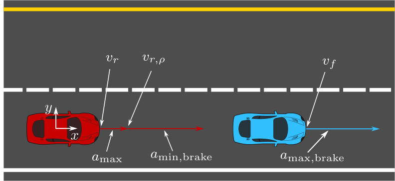
(a)

(b)

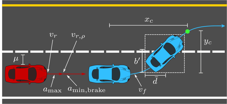
(c)

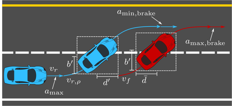
(d)

Figure 1: (a) The standard RSS braking manoeuvre for a braking leading vehicle. Velocity and acceleration arrows point to path segments where they occur. (b) The proposed swerve manoeuvre for a leading braking vehicle. The green dot represents the lateral clearance distance $y_{c}$ required by RSS. (c) The braking manoeuvre required for a swerving leading vehicle. (d) The swerving manoeuvre required for a swerving leading vehicle.

This paper aims to address the latter issue, especially as it pertains to the Responsibility-Sensitive Safety (RSS) framework [5]. Fundamental to the RSS framework is its assumption of responsibility, and that vehicles have a duty of care to one another. The assumption of responsible behaviour allows for the autonomous vehicle to make meaningful progress in the driving task. Under other frameworks that assume adversarial vehicles, the autonomous vehicle often exhibits over-conservative behaviour that impedes progress. This assumption of responsible behaviour allows for the computation of safe following distances such that vehicles can comfortably brake for a braking vehicle in front of them, without causing a collision. This following distance is a function of both vehicle’s speeds and maximum accelerations, as well as the reacting vehicle’s reaction time. When computing this following distance, the vehicles are modeled by a kinematic particle model. As long as this following distance is maintained by all vehicles, no collisions can occur.

This paper extends this framework to include swerve manoeuvres feasible for the kinematic bicycle model as a valid response, in addition to the standard braking response. In doing so, vehicles are able to follow at closer following distances at higher speeds, allowing for more efficient use of the road network. Using swerve manoeuvres feasible for the kinematic bicycle model ensures that these manoeuvres are more realistic than those possible under the particle model used in RSS.

I-A Contributions

The contributions in this paper are as follows. The first is the derivation of safe following distances in scenarios where vehicles perform swerve manoeuvres. In addition to the scenario of braking for a braking vehicle considered in RSS, we consider the additional scenarios of swerving for a braking vehicle, braking for a swerving vehicle, and swerving for a swerving vehicle. These distances are then used to form a novel extension of the RSS framework: a shorter following distance at high speeds. When all vehicles in a road network follow this new distance as well the rest of the RSS framework, and satisfy our assumptions, they are provably safe from collision.

The second contribution is a validation of our use of the kinematic bicycle model by comparing our swerve manoeuvres to manoeuvres generated under a dynamic single-track model [7]. As part of this dynamic model, we include a Pacejka tire model [8] to account for road surface traction. We show that the kinematic model, when lateral acceleration is constrained, can accurately estimate the longitudinal distance required to perform swerve manoeuvres using the dynamic model.

I-B Related Work

Previous work on swerve manoeuvres for autonomous driving have often focused on feasible manoeuvres according to various kinodynamic models [9]. In particular, many of these papers have assumed some variant of the bicycle model [10, 11, 12, 13] and performed optimization to generate optimal swerve manoeuvres. However, under these models the optimal solution is not generated through a closed form solution, which makes formally proving safety challenging.

Other work has instead simplified the vehicle model to a point mass model [14, 15, 16] in order to yield closed form, optimal solutions. However, this comes at the cost of the nonholonomic constraint present in the bicycle model, which result in manoeuvres that would be unrealistic for a car to execute. The goal with this work is to yield closed form, feasible solutions to swerve manoeuvre boundary condition problems, while still preserving the kinematic constraints that allow the manoeuvre to be executable by a real vehicle.

Previous work on using the kinematic bicycle model for autonomous driving has shown it is an effective model for tracking trajectories in MPC [17], and as such, contains important kinematic constraints that capture some of the limits of vehicle motion. Past work has also shown that the kinematic bicycle model is an accurate approximation to vehicle motion at low accelerations [18], which we expect to see as well in our validation.

II Preliminaries

II-A Responsibility-Sensitive Safety (RSS)

In this paper, we rely on two aspects of the RSS framework; the longitudinal and lateral safe distances required between two vehicles. In particular, we examine how the equivalent longitudinal safe distance for a swerve manoeuvre compares to that of a brake manoeuvre, while maintaining an appropriate lateral safe distance when required. In this work, we compare swerve manoeuvres moving to the left as in Figure 1, however, the same analysis can be applied to swerves moving to the right.

In RSS, safe distances are a function of several variables that describe the situation. The initial speed of the rear autonomous vehicle is given by $v_{r}$, and the initial speed of the front vehicle is denoted by $v_{f}$. The reaction time is given by $\rho$. The interpretation of the reaction time is the duration after which a vehicle can apply a mitigating action. During the reaction time, both vehicles apply the most dangerous acceleration possible, $a_{\max,\text{accel}}$, $a_{\max,\text{brake}}$ in the longitudinal case, and $a_{\max}^{\text{lat}}$ in the lateral case. To ensure passenger comfort, as well as to prevent tailgater safety issues, the mitigating reaction of the rear vehicle is assumed to be a comfortable deceleration, denoted $a_{\min,\text{brake}}$. This term comes from RSS, and is interpreted as the threshold for a safe, responsible braking response for the autonomous car. Note that these accelerations are magnitudes.

We denote the positive part of an expression with $[\cdot]_{+}$. Velocities are signed according to Figure 1a, and accelerations are unsigned parameters of the framework. If the post-reaction speeds $v_{r,\rho}$ and $v_{f,\rho}$ are given by

$$v_{r,\rho}=v_{r}+a_{\max,\text{accel}}\rho,$$ (1)

$$v_{r,\rho}^{\text{lat}}=v_{r}^{\text{lat}}-a_{\max}^{\text{lat}}\rho,$$ (2)

$$v_{f,\rho}^{\text{lat}}=v_{f}^{\text{lat}}+a_{\max}^{\text{lat}}\rho,$$ (3)

the longitudinal and lateral safe distances are given by

$$d_{\text{long}}=\biggl{[}v_{r}\rho+\frac{1}{2}a_{\max,\text{accel}}\rho^{2}+\\ \frac{(v_{r}+v_{r,\rho})^{2}}{2a_{\min,\text{brake}}}-\frac{v_{f}^{2}}{2a_{\max,\text{brake}}}\biggr{]}_{+},$$ (4)

$$d_{\text{lat}}=\mu+\biggl{[}-\left(\frac{v_{r}^{\text{lat}}+v_{r,\rho}^{\text{lat}}}{2}\right)\rho+\frac{(v_{r,\rho}^{\text{lat}})^{2}}{2a_{\min}^{\text{lat}}}+\\ \frac{v_{f}^{\text{lat}}+v_{f,\rho}^{\text{lat}}}{2}\rho+\frac{(v_{f,\rho}^{\text{lat}})^{2}}{2a_{\min}^{\text{lat}}}\biggr{]}_{+}.$$ (5)

The longitudinal safe distance is between the frontmost point of the rear vehicle and the rearmost point of the front vehicle along the longitudinal direction, and the lateral safe distance is between the rightmost point of the rear vehicle and the leftmost point of the front vehicle along the lateral direction. These are left implicit in the original RSS formulation, but since swerves involve rotation of the chassis, we make them explicit in this work. The longitudinal safe distance $d_{\text{long}}$ is the distance required such that the rear vehicle can maximally accelerate during its reaction time, then minimally decelerate to a stop, all while the front vehicle is maximally braking, without causing a collision. The lateral safe distance $d_{\text{lat}}$ is the distance required such that both vehicles can maximally accelerate towards each other during the reaction time $\rho$, then minimally decelerate until zero lateral velocity, while still maintaining at least a $\mu$ distance buffer.

When computing safety for swerve manoeuvres, the vehicle must maintain these safe distances with other relevant vehicles. These vehicles are relevant according to longitudinal and lateral adjacency, as defined below. We denote the vehicle dimensions $d_{f}$, $d_{r}$, $b_{l}$, $b_{r}$ as in Figure 3a.

Definition II.1.

If $x_{1}$, $x_{2}$ denote the longitudinal position of each vehicle, and then the vehicles are laterally adjacent if $x_{2}-d_{r}-d_{f}\leq x_{1}\leq x_{2}+d_{r}+d_{f}$.

Definition II.2.

If $y_{1}$, $y_{2}$ denotes the lateral position of each vehicle, then the vehicles are longitudinally adjacent if $y_{2}-b_{l}-b_{r}-d_{lat}\leq y_{1}\leq y_{2}+b_{l}+b_{r}+d_{lat}$.

Combining the definitions for safe distances and adjacency gives us a definition of safety.

Definition II.3.

A vehicle is laterally/longitudinally safe from another vehicle if it is not laterally/longitudinally adjacent to the other vehicle, or if it is laterally/longitudinally adjacent to the other vehicle and there is at least $d_{\text{lat}}$/$d_{\text{long}}$ of distance between them.

Definition II.4.

For a swerving vehicle and a non-swerving vehicle, as well as a given swerve manoeuvre, we define the lateral clearance distance, $y_{c}$, as the earliest point in the swerve at which the swerving vehicle is no longer longitudinally adjacent to the non-swerving vehicle.

In Figure 1, $y_{c}$ is reached at the green dot along the swerve. The lateral clearance distance allows us to compute the longitudinal distance covered by the swerve, which is denoted by $x_{c}$. We then use $x_{c}$ to compute the equivalent of $d_{\text{long}}$ for a swerve manoeuvre, and compare it to Equation 4.

II-B Vehicle Models

The analysis in this paper relies upon three different kinodynamic models. The first is the particle kinematic model, which is used in the RSS framework. Through all of these kinematic models, $x$ is longitudinal displacement and $y$ is lateral displacement. The control input is the acceleration in each dimension

$$\ddot{x}=a_{x}, \ddot{y}=a_{y}.$$ (6)

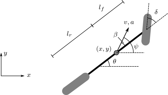
(a)

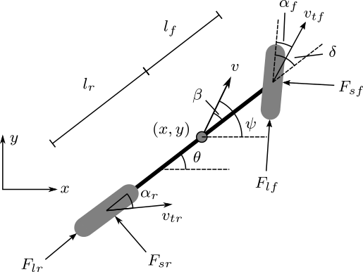
(b)

Figure 2: (a) The kinematic bicycle model, along with its associated variables. (b) The dynamic single track model used for validation [7]. Drag forces are omitted for simplicity, but are included in our computation.

When computing swerve manoeuvres, we wish to model the non-holonomic constraints on a car’s motion to make the manoeuvres realistic. To do so, we rely on the kinematic bicycle model, a model commonly used in autonomous driving [19, 20, 17]. This is illustrated in Figure 2a. In this model, $v$ is the velocity of the vehicle, $\psi$ is the heading of velocity at the centre of mass, $\theta$ is the yaw of the chassis, $\beta$ is the slip angle of the centre of mass relative to the chassis, $a$ is the input acceleration, $\delta$ is the input steering angle, $R_{c}$ is the turning radius of the center of mass, and $l_{r}$ and $l_{f}$ are the distances from the rear and front axle to the centre of mass, respectively

$$\dot{x} =v\cos(\psi+\beta), \beta =\tan^{-1}\left(\frac{l_{r}}{l_{r}+l_{f}}\tan(\delta)\right),$$

$$\dot{y} =v\sin(\psi+\beta), \theta =\psi-\beta,$$

$$\dot{\theta} =\frac{v\tan(\delta)}{l_{r}+l_{f}}, |\delta| \leq\delta_{\max}$$

$$\dot{v} =a, |a_{\text{lat}}| =\frac{v^{2}}{R_{c}}\leq a^{\text{lat}}_{\min},$$

$$R_{c} =\frac{l_{r}+l_{f}}{\cos(\beta)\tan(\delta)}, -a_{\text{brake},\min} \leq a\leq a_{\max}.$$ (7)

Finally, to verify our kinematic approximation is valid, we compare our swerve manoeuvres to those executed by a dynamic single-track vehicle model [7] with tires modelled using the Pacejka tire model [8]. This model is shown in Figure 2b. In this vehicle model, $v$, $\psi$, $\beta$, $\delta$, $l_{f}$, and $l_{r}$ are the same as the bicycle model. The slip angles of the front and rear tires are $\alpha_{f}$ and $\alpha_{r}$, respectively. The lateral tire forces on the front and rear tires are denoted $F_{\textit{sf}}$ and $F_{\textit{sr}}$, respectively, and $F_{\textit{lf}}$ and $F_{\textit{lr}}$ denote the longitudinal tire forces at the front and rear tires, respectively. The drag mount point is denoted $e_{\textit{SP}}$, and $F_{\textit{Ax}}$ and $F_{\textit{Ay}}$ are the longitudinal and lateral drag forces, respectively. The yaw rate is $\omega_{z}$, and $\omega_{\delta}$ is the input steering rate. The mass of the car is $m$, and $I_{\textit{zz}}$ is the inertia about the $z$-axis. We omit the equations of motion for brevity, but they are presented in the reference [7].

III Problem Formulation

The fundamental problem this paper addresses is to compute the longitudinal safe distance required when there is a free lane (or shoulder) to the left or right of the vehicle, allowing for an evasive swerve manoeuvre. This requires knowing the longitudinal safe distance required for the scenarios illustrated in Figure 1. As can be seen, when computing the longitudinal safe distances for swerves, one needs to consider both longitudinal and lateral clearance, since swerves involve lateral and longitudinal displacement.

Since vehicles rotate during swerves, rotation must be compensated for when computing these clearances. After compensating for rotation, the longitudinal swerve distance $x_{c}$ can then be used to compute the longitudinal safe distance required for a swerve. In RSS, safety was proved for a particle model. This paper extends those results to prove the safety for swerves feasible for the kinematic bicycle model. It is then shown how this result can be applied to more general models in Section V. This task then breaks down into five subproblems.

Subproblem 1. Given the initial speed of a swerving vehicle $v_{r}$, the vehicle dimensions $d_{f}$, $d_{r}$, $b_{l}$, $b_{r}$ as in Figure 3a, and parameters $\mu$ and $\rho$, compute a lateral clearance distance $y_{c}$ sufficient for lateral safety when a swerving vehicle becomes laterally adjacent to a lead vehicle.

Subproblem 2. Given the kinematic constraints in (II-B), the initial vehicle speeds $v_{r}$ and $v_{f}$, the lateral clearance distance $y_{c}$, and parameters $\rho$, $a_{\max}$, $a_{\min,\text{brake}}$, $a_{\max,\text{brake}}$, $a^{\text{lat}}_{\max}$, and $a^{\text{lat}}_{\min}$, compute a longitudinal safe distance sufficient for safety when swerving for a braking lead vehicle. This is illustrated in Figure 1b.

Subproblem 3. Given the initial vehicle speeds $v_{r}$ and $v_{f}$, the clearance point $y_{c}$, and parameters $\rho$, $a_{\max}$, $a_{\min,\text{brake}}$, $a^{\text{lat}}_{\max}$, and $a^{\text{lat}}_{\min}$, compute a longitudinal safe distance sufficient for safety when braking for a swerving lead vehicle. This is illustrated in Figure 1c.

Subproblem 4. Given the kinematic constraints in (II-B), the initial vehicle speeds $v_{r}$ and $v_{f}$, the parameters $\rho$, $a_{\max}$, $a_{\min,\text{brake}}$, $a_{\max,\text{brake}}$, $a^{\text{lat}}_{\max}$, and $a^{\text{lat}}_{\min}$, compute a longitudinal safe distance sufficient for safety when swerving behind a swerving lead vehicle. This is illustrated in Figure 1d.

Subproblem 5. Given longitudinal safe distance sufficient for safety when swerving for a braking vehicle, braking for a swerving lead vehicle, and swerving for a swerving lead vehicle, compute a longitudinal safe distance akin to $d_{\text{long}}$ that is sufficient for universal safety when maintained by all vehicles on the road.

The first subproblem is addressed in Section IV-A, the second in Section IV-B, the third in Section IV-C, the fourth in Section IV-D, and the fifth in Section IV-E.

The work in this paper makes the following assumptions on responsible behaviour:

1. A vehicle will only perform a swerve manoeuvre if it is not braking, and will only perform a brake manoeuvre if it is not swerving.

2. For every swerve manoeuvre, each vehicle reaches the lateral clearance distance only once. As a result, once a vehicle has committed to a lane change by reaching the lateral clearance distance, it will not return to its previous lane.

3. Each vehicle moves forward along the road, $v\geq 0$ and $\frac{-\pi}{2}\leq\psi\leq\frac{\pi}{2}$.

IV Computing the Longitudinal Safe Distance

IV-A Lateral Clearance Distance

To compute the lateral clearance distance $y_{c}$, we modify Equation (5) to account for vehicle rotation. If we know the maximum chassis yaw $\theta_{\max}$ during the manoeuvre, we can compute an axis-aligned bounding rectangle as an outer approximation to the vehicle footprint. This is useful for safety analysis, and is illustrated in Figure 3a.

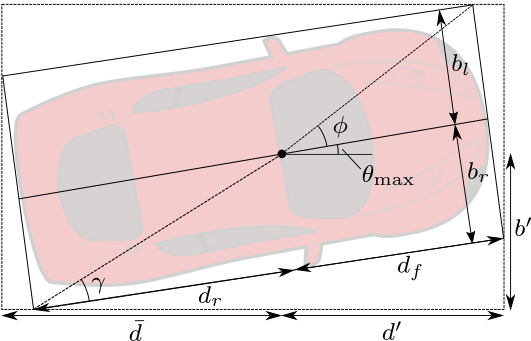
(a)

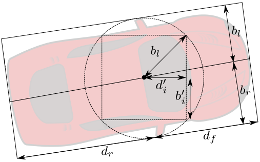
(b)

Figure 3: (a) An outer approximation to a vehicle chassis that rotates by $\theta_{\max}$. The distances $d^{\prime}$ and $\bar{d}$ are used for longitudinal buffers during swerve manoeuvres, and $b^{\prime}$ is used as a lateral buffer. (b) An inner approximation to a rotating vehicle chassis.

The three distances we need for safety analysis are from the centre of mass to the front of the bounding rectangle, $d^{\prime}$, from the centre of mass to the side of the bounding rectangle, $b^{\prime}$, and from the centre of mass to the rear of the bounding rectangle, $\bar{d}$. The distances from the centre of mass to the rear and front of the chassis are $d_{r}$ and $d_{f}$, respectively. The distances to the left and right of the chassis are $b_{l}$ and $b_{r}$, respectively. As the vehicle rotates, the length and width of the bounding rectangle increases until $\theta_{\max}$ reaches the angles from the centre of mass to the corners of the rectangle. Further rotation past these points decreases the dimensions of the bounding rectangle. We can write these angles in terms of $\phi$ and $\gamma$, illustrated in Figure 3a. The equations for the bounding rectangle distances are then $d^{\prime}$, $\bar{d}$, and $b^{\prime}$ are

$$d^{\prime}=\begin{cases}d_{f}\cos(\theta_{\max})+b_{r}\sin(\theta_{\max})&\theta_{\max}\leq\phi,\\ \sqrt{d_{f}^{2}+b_{r}^{2}}&\theta_{\max}>\phi,\end{cases}$$ (8)

$$\bar{d}=\begin{cases}d_{r}\cos(\theta_{\max})+b_{l}\sin(\theta_{\max})&\theta_{\max}\leq\gamma,\\ \sqrt{d_{r}^{2}+b_{l}^{2}}&\theta_{\max}>\gamma,\end{cases}$$ (9)

$$b^{\prime}=\begin{cases}d_{r}\sin(\theta_{\max})+b_{r}\cos(\theta_{\max})&\theta_{\max}\leq\frac{\pi}{2}-\gamma,\\ \sqrt{d_{r}^{2}+b_{r}^{2}}&\theta_{\max}>\frac{\pi}{2}-\gamma.\end{cases}$$ (10)

We now have an expression for the bounding rectangle distances of a rotating vehicle in terms of $\theta_{\max}$, which is computed in Section IV-B.

Using $b^{\prime}$ and the lateral safe distance $d_{\text{lat}}$, we can now compute the lateral clearance distance, $y_{c}$ required for Subproblem 1.

$$y_{c}=b^{\prime}+b_{l}+d_{\text{lat}}.$$ (11)

Let us denote the time $y_{c}$ is attained as $t_{c}$.

Theorem 1.

Equation 11 gives a lateral clearance distance sufficient for lateral safety when a swerving vehicle becomes laterally adjacent to another braking vehicle, or any time before.

Proof.

To show lateral safety, we must show that laterally adjacent vehicles are at least $d_{\text{lat}}$ from one another, as given in Equation 5. Since the swerving vehicle’s lateral speed is variable but nonnegative, a conservative lower bound on its lateral velocity is zero when computing $d_{\text{lat}}$. From assumption 1, since the other vehicle is braking, it is not swerving, and therefore has zero lateral velocity during the swerve. The required $d_{\text{lat}}$ can then be computed using Equation 5, taking $v_{r}^{\text{lat}}$ and $v_{f}^{\text{lat}}$ to be zero, and using the parameters $a^{\text{lat}}_{\min}$, $a^{\text{lat}}_{\max}$, and $\rho$. The distance $d_{\text{lat}}$ acts as a buffer to ensure that upon reaching lateral adjacency, both agents are laterally safe from one another.

For $t<t_{c}$, the swerving vehicle is not laterally adjacent to the other vehicle, and is laterally safe. For $t\geq t_{c}$, from Assumption 2, $t_{c}$ is the time at which the two vehicles are closest while laterally adjacent. From Equation 11, there is at least $d_{\text{lat}}$ of distance between the vehicles, and thus they are laterally safe $\forall t\geq t_{c}$. ∎

IV-B Swerving for a Braking Vehicle

We can now use $y_{c}$ to compute the longitudinal safe distance, $d_{\textit{s,b}}$, required when swerving to avoid a braking lead vehicle. We wish to do so under the constraints of the bicycle model outlined in Section II-A. In addition, if $\alpha$ denotes the lane width, $t_{f}$ denotes the end time of the swerve, and the origin of the coordinate frame is at the center line of the current lane at the rear vehicle’s position at $t=0$, we would like the swerve to satisfy the following boundary conditions:

$$\theta(t_{f})=0,~{}y(t_{f})=\alpha.$$ (12)

However, to compute the optimal swerve manoeuvre with respect to longitudinal clearance is an optimization problem with no closed form solution [11]. Instead, we can compute a swerve manoeuvre feasible for the bicycle model, and use that to obtain an upper bound on the actual longitudinal distance required by a swerve constrained by the bicycle model.

As in Equation 4, the lead vehicle is travelling with velocity $v_{f}$, and then brakes at $a_{\max,\text{brake}}$ during the entire manoeuvre. The swerve is preceded by the rear vehicle maximally accelerating during the reaction delay $\rho$, at which point it begins the swerve manoeuvre with initial speed $v_{r,\rho}$. To ensure monotonicity in the gap between the rear and lead vehicles, a lower bound on the distance travelled until $t_{f}$ by the lead vehicle is used, denoted $x_{f}$.

The swerve we consider is bang-bang in the steering input with zero longitudinal acceleration, and is illustrated in Figure 4. We denote the longitudinal distance travelled by the swerving vehicle until the swerving vehicle reaches the lateral clearance distance as $x_{c}$ This distance $x_{c}$ is computed in Equations 21 and 26.

For the swerve manoeuvre, the turning radius of the circular arcs depends on the maximum lateral acceleration, as well as the kinematic limits of the steering angle. The constraints on steering angle and lateral acceleration from (II-B) give two constraints on the turning radius

$$R_{\min,\delta}=\sqrt{\frac{(l_{r}+l_{f})^{2}}{\tan(\delta_{\max})^{2}+l_{r}^{2}}}, R_{\min,a}=\frac{v_{r,\rho}^{2}}{a^{\text{lat}}_{\min}}.$$ (13)

To ensure both constraints are satisfied, we set $R_{c}$ from (II-B) to the maximum of the two. From this turning radius, we can compute the steering angle $\delta_{c}$ and the slip angle $\beta_{c}$

$$\delta_{c}=\tan^{-1}\left(\sqrt{\frac{(l_{r}+l_{f})^{2}}{R_{c}^{2}-l_{r}^{2}}}\right), \beta_{c}=\tan^{-1}\left(\frac{l_{r}\tan(\delta_{c})}{l_{r}+l_{f}}\right).$$ (14)

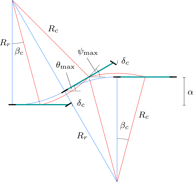
Figure 4: The swerve manoeuvre used for safety analysis. The red path is taken by the centre of mass, and the blue path is taken by the rear axle. The distance between lanes is $\alpha$, $\delta_{c}$ is the steering angle, $\beta_{c}$ is the slip angle. The maximum angles achieved by the chassis yaw and the velocity of the centre of mass are given by $\theta_{\max}$ and $\psi_{\max}$, respectively. The turning radius of the rear axle and centre of mass’s paths are given by $R_{r}$ and $R_{c}$, respectively.

We can now compute the $\theta_{\max}$ required to satisfy the boundary conditions in  Equation 12. From the rear axle, the two circular arcs are symmetrical in lateral distance travelled, as in Figure 4. Therefore, we can compute the angle along the first circular arc required to reach a lateral distance of $\frac{\alpha}{2}$. First, we compute the turning radius at the rear axle, $R_{r}$

$$R_{r}=\frac{l_{r}+l_{f}}{\tan(\delta_{c})}.$$ (15)

The lateral distance travelled during the first circular arc is then given by

$$y(t)=R_{r}(1-\cos(\theta(t))).$$ (16)

For a given value of $\delta_{c}$, $\theta_{\max}$ is then

$$\theta_{\max}=\cos^{-1}\left(1-\frac{\alpha}{2R_{r}}\right).$$ (17)

To compute $x_{c}$, there are two cases, depending on if $y_{c}$ is reached in the first or second circular arc. We can compute $\psi_{\max}$ using (II-B). From Assumption 3, we have that $\psi_{\max}\leq\frac{\pi}{2}$. Thus, the first case occurs if

$$y_{c}\leq R_{c}(\cos(\beta_{c})-\cos(\psi_{\max})),$$ (18)

otherwise the second case occurs.

IV-B1 First Circular Arc

Similar to Equation 16, the longitudinal position along the first circular arc is given by

$$x(t)=R_{c}(\sin(\psi(t))-\sin(\beta_{c})).$$ (19)

We can use the centre of mass equivalent of Equation 16 and $y_{c}$ to compute the $\psi$ value at the clearance point, $\psi_{c}$

$$\psi_{c}=\cos^{-1}\left(\cos(\beta_{c})-\frac{y_{c}}{R_{c}}\right).$$ (20)

Substituting this value for $\psi$ in Equation 19 gives our swerve longitudinal distance

$$x_{c}=R_{c}(\sin(\psi_{c})-\sin(\beta_{c})).$$ (21)

The magnitude of the velocity is constant during the swerve, and so we can compute $t_{c}$ using the arc length travelled up to the clearance point $y_{c}$,

$$t_{c}=\frac{R_{c}(\psi_{c}-\beta_{c})}{v}.$$ (22)

IV-B2 Second Circular Arc

In the second circular arc, we denote the initial heading of the centre of mass as $\hat{\psi}=\psi_{\max}-2\beta_{c}$, the initial $x$ position as $\hat{x}=R_{c}(\sin(\psi_{\max})-\sin(\beta_{c}))$, and the initial $y$ position as $\hat{y}=R_{c}(\cos(\beta_{c})-\cos(\psi_{\max})$. The longitudinal and lateral distance along this arc are then

$$x(t)=R_{c}(\sin(\hat{\psi})-\sin(\psi(t)))+\hat{x},$$ (23)

$$y(t)=R_{c}(\cos(\psi(t))-\cos(\hat{\psi}))+\hat{y}.$$ (24)

As in Case 1, substituting $y_{c}$ gives us $\psi_{c}$,

$$\psi_{c}=\cos^{-1}\left(\frac{1}{R_{c}}\left(y_{c}-\hat{y}\right)+\cos(\hat{\psi})\right)$$ (25)

Substituting this value for $\psi$ in Equation 23 and add $d^{\prime}$ gives

$$x_{c}=R_{c}(\sin(\hat{\psi})-\sin(\psi_{c}))+\hat{x}+d^{\prime}.$$ (26)

Similar to Case 1, we can then compute the clearance time $t_{c}$,

$$t_{c}=\frac{R_{c}(\psi_{\max}-\beta_{c}+\hat{\psi}-\psi_{c})}{v}.$$ (27)

From these longitudinal swerve clearance values, we can then compute the longitudinal safe distance. To do this, we can replace the rear braking distance in Equation 4 with the longitudinal swerve distance $x_{c}$. In addition, to ensure a monotonically decreasing gap between the two vehicles, we set the initial speed of the lead vehicle (as a conservative approximation) to

$$v_{f}^{\prime}=\min(v_{f},v_{r}\cos(\psi_{\max})).$$ (28)

The braking distance of the lead vehicle occurs during the reaction time $\rho$ and the swerve clearance time $t_{c}$, giving a front vehicle braking distance of

$$x_{f}=v_{f}^{\prime}(\rho+t_{c})-\frac{a_{\max,\text{brake}}(\rho+t_{c})^{2}}{2}.$$ (29)

Using the parameters $a_{\max,\text{accel}},\rho$ introduced in Section II-A, the longitudinal safe distance between a swerving rear vehicle and a braking lead vehicle is

$$d_{\textit{s,b}}=\biggl{[}v_{r}\rho+\frac{1}{2}a_{\max,\text{accel}}\rho^{2}+x_{c}-x_{f}\biggr{]}_{+}+d^{\prime}+d.$$ (30)

Theorem 2.

Equation 30 gives a longitudinal safe distance sufficient for safety when swerving for a braking lead vehicle.

Proof.

For $t>t_{c}$, $y(t)>y_{c}$, and therefore the swerving vehicle is no longer longitudinally adjacent to the lead vehicle, so is safe from the lead vehicle’s braking. For $t\leq t_{c}$, from Equation 28, we use a conservative lower bound for the speed of the lead vehicle to ensure the lead vehicle’s speed is less than the swerving vehicle during the entire swerve. This implies the gap between the two vehicles is monotonically decreasing. This means the minimum gap between the two vehicles occurs at time $t_{c}$.

The swerving vehicle travels $x_{c}+v_{r}\rho+\frac{1}{2}a_{\max,\text{accel}}\rho^{2}$, and a conservative lower bound on the lead vehicle’s travel distance is $v_{f}^{\prime}(\rho+t_{c})-\frac{1}{2}a_{\max,\text{brake}}(\rho+t_{c})^{2}$. There is at most $d^{\prime}$ of distance from the centre of mass to the front of the swerving vehicle. Thus, if a swerving vehicle maintains distance $d_{\textit{s,b}}$, it is safe from the lead vehicle at time $t_{c}$. Since the gap is monotonically decreasing for $t\leq t_{c}$, it is safe $\forall t\leq t_{c}$.

∎

IV-C Braking for a Swerving Vehicle

The longitudinal safe distance required to swerve for a braking vehicle was computed in the preceding section, and this section considers the opposite problem, computing the longitudinal safe distance required to brake for a swerving lead vehicle without collision. Since the lead vehicle intends to occupy the other lane, it requires less longitudinal distance for the rear vehicle to brake to avoid the swerving lead vehicle than it would for it to brake for a braking lead vehicle. It is assumed the front vehicle is performing the same swerve discussed in Section IV-B. To account for rotation of the front vehicle, $\bar{d}$ is used to compensate as defined in Section IV-A.

Equations 21, 22, 21, and 27 can be used to compute the $x_{c}$ and $t_{c}$ for the front vehicle’s swerve. As in Equation 4, it is assumed that the rear vehicle accelerates maximally during its reaction time, and then brakes comfortably until $t_{c}$. As before, denote the rear vehicle’s post-acceleration velocity as $v_{r,\rho}$. Then its minimum velocity during the braking manoeuvre is

$$v_{r,\min}=\max(\min(v_{r},v_{r,\rho}-a_{\min,\text{brake}}(t_{c}-\rho)),0).$$ (31)

As in Section IV-B, the proof of safety is simplified if the gap is monotonically decreasing until lateral safety is reached. To ensure this, the lead vehicle speed is conservatively bounded with $v_{f}^{\prime}$

$$v_{f}^{\prime}=\min(v_{f}\cos(\psi_{\max}),v_{r,\min}).$$ (32)

A conservative lower bound for the longitudinal distance travelled by the swerving front vehicle is then

$$x_{f}=v_{f}^{\prime}t_{c}.$$ (33)

The distance $x_{f}$ is a lower bound on the distance travelled by the front vehicle during the swerve that creates a monotonically decreasing gap.

The distance travelled by the rear braking vehicle during its reactions delay and its braking manoeuvre is denoted by $x_{r}$. This distance depends on the clearance time $t_{c}$, similar to the distance travelled by the front vehicle in the preceding section. The distance travelled during the rear vehicle’s braking manoeuvre, $x_{r,\text{brake}}$, is given by

$$x_{r,\text{brake}}=\begin{cases}v_{r,\rho}(t_{c}-\rho)-\frac{a_{\min,\text{brake}}(t_{c}-\rho)^{2}}{2},&t_{c}-\rho\leq\frac{v_{r,\rho}}{a_{\min,\text{brake}}},\\ \frac{v_{r,\rho}^{2}}{2a_{\min,\text{brake}}},&t_{c}-\rho>\frac{v_{r,\rho}}{a_{\min,\text{brake}}}.\end{cases}$$ (34)

Following this, the distance travelled by the braking rear vehicle is

$$x_{r}=\frac{(v_{r}+v_{r,\rho})\rho}{2}+x_{r,\text{brake}}.$$ (35)

Using Equations 33 and 35, the longitudinal safe distance when braking for a swerving vehicle, $d_{\textit{b,s}}$ is then

$$d_{\textit{b,s}}=\left[x_{r}-x_{f}\right]_{+}+d_{f}+\bar{d}.$$ (36)

Theorem 3.

Equation 36 gives a longitudinal safe distance sufficient for safety when braking for a swerving lead vehicle.

Proof.

For $t>t_{c}$, the swerving vehicle is laterally clear from the rear braking vehicle, and therefore the rear vehicle is safe. The velocity used for the lead vehicle is a conservative lower bound on its true speed $\forall t\leq t_{c}$, as per Equation 32. In addition, $v_{f}^{\prime}\leq v_{r}$, $\forall t\leq t_{c}$, and as a result the gap between the two vehicles is monotonically decreasing on that interval. The minimum distance between the two vehicles thus occurs at time $t_{c}$. Equation 36 thus gives enough clearance such that no collision occurs at time $t_{c}$, so the rear vehicle is safe at time $t_{c}$. Since the gap is monotonically decreasing over the interval, the rear vehicle is safe $\forall t\leq t_{c}$. ∎

IV-D Swerving for a Swerving vehicle

The final relevant longitudinal safe distance is the distance required when swerving behind a swerving lead vehicle. This is illustrated in Figure 1d. Both vehicles are longitudinally adjacent during the entire manoeuvre. From Assumption 1, the lead vehicle will not brake during its swerve. The goal is then to compute the longitudinal distance required to swerve behind a lead swerving vehicle, such that if the lead vehicle were to immediately brake with deceleration $a_{\max,\text{accel}}$ at the end of its swerve, and the rear vehicle were to brake with deceleration $a_{\min,\text{accel}}$ at the end of its reaction-delayed swerve, there would be no collision. The swerve completion times of the rear and front vehicle are given by $t_{1}$ and $t_{2}$, respectively. Similar to the previous section, $v_{f}^{\prime}$ denotes a conservative lower bound on the front vehicle’s speed. The longitudinal safe distance required to swerve in response to a swerving vehicle, $d_{\textit{s,s}}$, is then

$$d_{\textit{s,s}}=\frac{v_{r}+v_{r,\rho}}{2}\rho+v_{r,\rho}(t_{1}-\rho)+\\ \frac{v_{r,\rho}^{2}}{2a_{\min,\text{brake}}}-\left(v_{f}^{\prime}t_{2}+\frac{v_{f}^{\prime 2}}{2a_{\max,\text{brake}}}\right)+d^{\prime}+\bar{d}.$$ (37)

Theorem 4.

Equation 37 gives a longitudinal safe distance sufficient for safety when swerving for a swerving lead vehicle.

Proof.

The gap between each vehicle can be written as a piecewise function of time. The endpoints of the intervals are functions of the reaction delay, $\rho$, the duration of the front vehicle’s swerve, $t_{2}$, the duration of the rear vehicle’s swerve, $t_{1}$, the brake time of the front vehicle, $t_{b,2}$, and the brake time of the rear vehicle, $t_{b,1}$. The swerve times for the kinematic bicycle model for varying speeds are proportional to $v\cos^{-1}\left(1-\frac{1}{v^{2}}\right)$, which is quasi-constant across all relevant road speeds. In addition, $a_{\max,\text{accel}}>a_{\min,\text{accel}}$, and swerve times are longer than reasonable reaction times. From this, it is reasonable to assume that the interval endpoints are $\rho<t_{2}<\rho+t_{1}<t_{2}+t_{b,2}<\rho+t_{1}+t_{b,1}$. Denote the longitudinal distance travelled during the swerves by the front and rear vehicle as $x_{s,2}(t)$ and $x_{s,1}(t)$ respectively, the initial gap between the vehicles by $g_{0}$, and the gap between the vehicles as $g(t)$.

The maximum longitudinal velocity during the rear vehicle swerve is $v_{r,\rho}$. If the maximum $\psi$ value during the front vehicles swerve is denoted $\psi_{\max,f}$, the minimum longitudinal velocity during the front vehicle’s swerve is given by $v_{f}\cos(\psi_{\max,f})$. Set $v_{f}^{\prime}=\min(v_{f}\cos(\psi_{\max,f}),v_{r})$. This means that

$$x_{s,1}(t)\leq v_{r,\rho}t,$$ (38)

$$x_{s,2}(t)\geq v_{f}^{\prime}t.$$ (39)

Using Equations 38 and 39 as conservative bounds on the distance travelled by both vehicles during the swerve manoeuvre results in a monotonically decreasing function of $t$, $\hat{g}(t)$, with the property that $\hat{g}(t)\leq g(t),\forall t$.

This implies that the minimum of $\hat{g}(t)$ occurs for $t>t_{b,1}$, where $\hat{g}(t)$ is constant

$$\min_{t}\hat{g}(t)=g_{0}+v_{f}^{\prime}t_{2}+\frac{v_{f}^{\prime 2}}{2a_{\max,\text{brake}}}-\\ ~{}~{}~{}~{}\left(\frac{v_{r}+v_{r,\rho}}{2}\rho+v_{r,\rho}t_{1}+\frac{v_{r,\rho}^{2}}{2a_{\min,\text{brake}}}\right).$$ (40)

Since $\hat{g}(t)\leq g(t),\forall t$, if $\hat{g}(t)\geq 0,\forall t$, no collision occurs. This is satisfied if the initial gap satisfies

$$g_{0}\geq\frac{v_{r}+v_{r,\rho}}{2}\rho+v_{r,\rho}t_{1}+\frac{v_{r,\rho}^{2}}{2a_{\min,\text{brake}}}-\\ ~{}~{}~{}~{}\left(v_{f}^{\prime}t_{2}+\frac{v_{f}^{\prime 2}}{2a_{\max,\text{brake}}}\right).$$ (41)

By adding in the distances from the centre of mass to the ends of the chassis, compensating for the rotation of each swerving vehicle, an initial gap is sufficient for safety $\forall t$ if

$$g_{0}\geq\frac{v_{r}+v_{r,\rho}}{2}\rho+v_{r,\rho}t_{1}+\frac{v_{r,\rho}^{2}}{2a_{\min,\text{brake}}}-\\ ~{}~{}~{}~{}\left(v_{f}^{\prime}t_{2}+\frac{v_{f}^{\prime 2}}{2a_{\max,\text{brake}}}\right)+d^{\prime}+\bar{d}.$$ (42)

Which yields Equation 37.

At $t\geq t_{2}$, the time at which the lead vehicle begins hard braking, there is enough longitudinal distance to brake for the leading vehicle, as $\hat{g}(t)\geq 0,\forall t\geq t_{2}$, so the rear vehicle is safe. Since $\hat{g}(t)$ is monotonically decreasing with respect to $t$, the safe longitudinal distance is satisfied for $t<t_{2}$, and thus the rear vehicle is safe $\forall t$. ∎

IV-E Universal Following Distance

The final subproblem addressed in this paper aims to combine the results of the previous sections into a final following distance that can be maintained by all vehicles in a given straight road system to ensure universal safety, assuming the vehicles can brake or swerve as a response to the behaviour of other vehicles in front of them. In this sense, this section extends the analysis of the preceding sections into the case of more than two vehicles in a road system. Each vehicle’s following distance will be a function of the speed of the vehicle, as well as the speed of the 2 vehicles in front of the vehicle, and the parameters outlined in Section II-A. Denote the distance required to brake for a braking lead vehicle as $d_{\textit{b,b}}(v_{r},v_{f},\rho)$, the distance required to swerve for a braking lead vehicle as $d_{\textit{b,s}}(v_{r},v_{f},\rho)$, the distance required to swerve for a braking lead vehicle as $d_{\textit{s,b}}(v_{r},v_{f},\rho)$, and the distance required to swerve for a swerving lead vehicle as $d_{\textit{s,s}}(v_{r},v_{f},\rho)$.

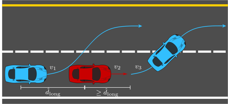
(a)

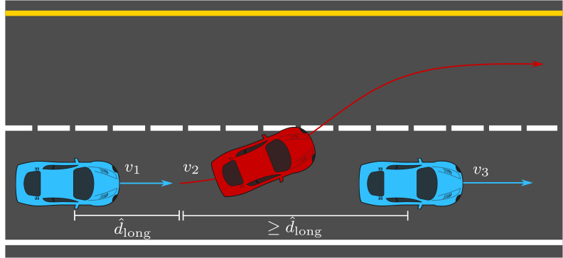
(b)

Figure 5: (a) Scenario where the rear vehicle must swerve for a swerving vehicle 2 cars ahead. (b) Scenario where the rear vehicle must brake for a braking vehicle 2 cars ahead.

In such a road system, there will be blocks of vehicles where the front vehicle in the block is much farther away from the nearest vehicle in front of it than both $d_{\textit{b,b}}$ and $d_{\textit{s,s}}$. Since it is at least this far, it can safely brake or swerve for any vehicle in front of it, and therefore any vehicle in front of it can be ignored. Because of this, these blocks can be considered in isolation, and if each block of vehicles is considered safe, then all vehicles in the road system are considered safe. For any vehicle in a given block, denote its speed by $v_{1}$, and the speeds of the first and second vehicles in front of it (if they exist within the block) as $v_{2}$ and $v_{3}$, respectively. The longitudinal position of each vehicle as a function of time is denoted by $x_{1}(t)$, $x_{2}(t)$, and $x_{3}(t)$. A sufficient safe following distance for each vehicle is then

$$\hat{d}_{\text{long}}=\max(d_{\textit{b,s}}(v_{1},v_{2},\rho),d_{\textit{b,s}}(v_{1},v_{2},\rho),\\ d_{\textit{s,s}}(v_{1},v_{3},2\rho)-d_{\textit{s,b}}(v_{2},v_{3},\rho),\\ d_{\textit{b,b}}(v_{1},v_{3},2\rho)-d_{\textit{s,b}}(v_{2},v_{3},\rho)).$$ (43)

Theorem 5.

Equation 43 gives a longitudinal safe distance sufficient for universal safety when maintained by all vehicles.

Proof.

As mentioned earlier, each block of vehicles can be analyzed individually for safety, and if every block is safe, all vehicles are safe. The safety of any given block can be proved using an inductive argument across all of the vehicles, starting from the front of the block. The following is a proof sketch.

• For the base case, the safety of the first two vehicles is proven when following with at least $\hat{d}_{\text{long}}$.

• For the inductive step, it is assumed the $i^{\text{th}}$ agent is following with at least $\hat{d}_{\text{long}}$ and is safe, and it is shown that if the $(i+1)^{\text{th}}$ agent follows with at least $\hat{d}_{\text{long}}$, then it is safe.

IV-E1 Base Case

The first vehicle at the front of the block is by definition at least $d_{\textit{b,b}}$ and $d_{\textit{s,s}}$ from any vehicle in front of it (if such a vehicle exists). As a result, any potential vehicle in front of the first can be safely avoided if necessary with either a brake or a swerve. This means that the first vehicle in the block is safe, and any potential vehicle in front of the first can be safely ignored by all vehicles in the block.

The second vehicle follows the first vehicle at $\hat{d}_{\text{long}}$. If the front vehicle brakes, the second vehicle is at least $d_{\textit{s,b}}$ away from it, and can swerve to safety. If the front vehicle swerves, the second vehicle is at least $d_{\textit{b,s}}$ away from it, and can brake safely. The second vehicle will therefore not collide with the first vehicle, and is therefore safe.

IV-E2 Induction

Now, suppose the $i^{\text{th}}$ vehicle is following with at least $\hat{d}_{\text{long}}$ of distance, and is safe from the vehicles in front of it. Denote the $(i+1)^{\text{th}}$ as vehicle 1, the $i^{\text{th}}$ vehicle as vehicle 2, and the $(i-1)^{\text{th}}$ vehicle as vehicle 3. The distance between vehicle 1 and vehicle 2 is $\hat{d}_{\text{long}}$. If vehicle 2 brakes or swerves, vehicle 1 is at least $d_{\textit{s,b}}$ and $d_{\textit{b,s}}$ away from it, and is safe from vehicle 2 if it responds with a swerve or brake, respectively.

If vehicle 1 swerves in response to vehicle 2’s brake, there are 2 cases to consider. The first case is if vehicle 3 was braking. Since vehicle 2 was assumed to be safe from vehicle 3, $x_{2}(t)\leq x_{3}(t),\forall t$. Combining this with the fact that $d_{\textit{s,b}}$ is sufficient for vehicle 1 to swerve safely from vehicle 2, vehicle 1 must be safe from vehicle 3 if vehicle 3 brakes.

If vehicle 3 was swerving, $d_{\textit{s,s}}(v_{1},v_{3},2\rho)$ is a sufficient distance for vehicle 1 to follow vehicle 3 to ensure safety. This case is illustrated in Figure 5a. The reaction delay is doubled to account for the reaction propagating through 2 vehicles instead of the usual one. Since vehicle 2 was assumed to be safe from vehicle 3, $d_{\textit{s,b}}(v_{2},v_{3},\rho)$ is a lower bound on vehicle 2’s following distance from vehicle 3. This means that in this case, $d_{\textit{s,s}}(v_{1},v_{3},2\rho)-d_{\textit{s,b}}(v_{2},v_{3},\rho)$ is a sufficient following distance between vehicle 1 and 2 to guarantee safety.

If vehicle 1 brakes in response to vehicle 2’s swerve, as before there are 2 cases to consider. The first case is if vehicle 3 was swerving. As before, since vehicle 2 was assumed to be safe from vehicle 3, $x_{2}(t)\leq x_{3}(t),\forall t$. Combining this with the fact that $d_{\textit{b,s}}$ is sufficient for vehicle 1 to brake safely from vehicle 2’s swerve, vehicle 1 must be safe from vehicle 3’s swerve.

If vehicle 3 was braking, $d_{\textit{b,b}}(v_{1},v_{3},2\rho)$ is a sufficient distance for vehicle 1 to follow vehicle 3 to ensure safety. This case is illustrated in Figure 5b. Again, the reaction delay is doubled to account for propagation between two vehicles. Since vehicle 2 was assumed to be safe from vehicle 3, $d_{\textit{s,b}}(v_{2},v_{3},\rho)$ is again a lower bound on vehicle 2’s following distance. Thus, in this case, $d_{\textit{b,b}}(v_{1},v_{3},2\rho)-d_{\textit{s,b}}(v_{2},v_{3},\rho)$ is a sufficient following distance between vehicle 1 and 2 to guarantee safety.

Since $\hat{d}_{\text{long}}$ is greater or equal to each of these following distances, vehicle 1 is safe, and thus the $(i+1)^{\text{th}}$ is safe. By induction, any block of vehicles where each vehicle maintains the following distance given in Equation 43 is safe, and as a result, the entire system is safe. ∎

At high speeds, this new following distance can be used to allow for tighter following between agents. At low speeds, the agents can revert to the braking following distance used in RSS.

If the positions of vehicles 2 and 3, $d_{2}$ and $d_{3}$ respectively, are known as well as their speeds, the following distance can be improved further. If we denote $d_{2,3}=d_{3}-d_{2}$, then by the same logic in the preceding proof, a sufficient longitudinal safe distance is

$$\hat{d}_{\text{long}}=\max(d_{\textit{b,s}}(v_{1},v_{2},\rho),d_{\textit{b,s}}(v_{1},v_{2},\rho),\\ d_{\textit{s,s}}(v_{1},v_{3},2\rho)-d_{2,3},d_{\textit{b,b}}(v_{1},v_{3},2\rho)-d_{2,3}).$$ (44)

A comparison between the RSS following distance and these new following distances across a range of speeds is shown in Figure 8. In the plot, all vehicles are moving at the same speed. Since $d_{2,3}$ can vary, for illustration purposes we assume each vehicle follows the agent in front of it at

$$\hat{d}_{\text{long}}=\max(d_{\textit{b,s}}(v_{1},v_{2},\rho),d_{\textit{b,s}}(v_{1},v_{2},\rho),\\ \frac{d_{\textit{s,s}}(v_{1},v_{3},2\rho)}{2},\frac{d_{\textit{b,b}}(v_{1},v_{3},2\rho)}{2}).$$ (45)

This results in a uniform following distance across all agents when they are moving at the same speed.

V Validation and Results

To validate our bicycle model assumptions, we first check the validity of our conservative upper bound on the required swerve distance by computing a lower bound. We then use a dynamic vehicle model [7] to see if our computed swerve distances are reasonable approximations. The lower bound is computed and compared to the upper bound distance, as well as the relevant braking distance, in Section V-A. In Section V-B, we compare our swerve clearance distance, as computed in Section IV-B, to swerves from the dynamic model.

V-A Lower Bound Validation

To compute a lower bound on the longitudinal swerve clearance distance $x_{c}$, we use the particle model in Equation 6. We set the minimum $a_{x}$ and maximum $a_{y}$ values to be $-a_{\min,\text{brake}}$ and $a_{\min}^{\text{lat}}$, respectively, from the bicycle model. This ensures that any acceleration possible under the bicycle model is also possible under the particle model.

For a particle model, maximal lateral acceleration towards $y_{c}$ as well as maximal longitudinal deceleration leads to lateral clearance in the shortest longitudinal distance $\bar{x}_{c}$ [14]. Thus, we have that $\bar{x}_{c}\leq x_{c}$ for any other manoeuvre feasible for the particle model.

Finally, for computing the clearance, we use an inner approximation of the vehicle’s chassis during rotation. To do so, we use the square inscribed on the circle of radius $b_{l}$ centred on the centre of mass with side length $2d_{i}^{\prime}$. This is shown in Figure 3b. Through this inner approximation, we have that $d_{i}^{\prime}\leq d^{\prime}$ for any possible chassis rotation. This implies that anything the chassis can clear during the swerve will be cleared by the inner square. If we use $x_{f}$ as in Section IV-B, a lower bound on the longitudinal safe distance, denoted by $\bar{d}_{\text{long}}$, is given by

$$\bar{d}_{\text{long}}=v_{r}\rho+\frac{1}{2}a_{\max,\text{accel}}\rho^{2}+\bar{x}_{c}-x_{f}.$$ (46)

Theorem 6.

Equation 46 gives a longitudinal safe distance necessary for safety when swerving for a braking lead vehicle.

Proof.

The clearance time and associated longitudinal distance at which point the particle model reaches $y_{c}$ are given by

$$t_{c}=\sqrt{\frac{2y_{c}}{a^{\text{lat}}_{\min}}}, \bar{x}_{c}=vt_{c}-\frac{a_{\min,\text{brake}}t_{c}^{2}}{2}+d_{i}^{\prime}.$$ (47)

By the acceleration constraints imposed on the particle model, any feasible acceleration in the bicycle model is feasible for the particle model. In addition, the manoeuvre is optimal with respect to longitudinal distance travelled for the particle model. Both of these points imply that the $\bar{x}_{c}$ in Equation 47 is a lower bound on any feasible $x_{c}$ for the bicycle model. Next, the inner approximation implies that for any manoeuvre, if the chassis can clear, the square with side length $2d_{i}^{\prime}$ can clear as well, allowing a buffer of $d_{i}^{\prime}$ to be added.

If we denote the initial longitudinal distance between the vehicles as $x_{2}$, then the distance between the swerving vehicle and the braking vehicle during the reaction delay is given by $x_{2}-d_{i}^{\prime}-d_{r}+v_{f}t-\frac{1}{2}a_{\max,\text{brake}}t^{2}-v_{r}t-\frac{1}{2}a_{\max}t^{2}$. If we denote the distance between the vehicles at the end of the reaction delay as $x_{\rho}$, then after the reaction delay the distance between the vehicles is given by $x_{\rho}+v_{f}t-\frac{1}{2}a_{\max,\text{brake}}t^{2}-v_{r,\rho}t+\frac{1}{2}a_{\min,\text{brake}}t^{2}$. Since $-a_{\max,\text{brake}}-a_{\max}<0$ and $-a_{\max,\text{brake}}+a_{\min,\text{brake}}<0$, the distance between the swerving and braking vehicle is concave on both intervals. This implies that the minimum gap occurs at the boundaries of the time intervals $\{0,\rho,t_{c}\}$. Since the distance between the vehicles is differentiable everywhere, the time $\rho$ is a critical point only if the derivative is zero. In this case, since the distance is concave before and after time $\rho$, the derivative is positive for $t<\rho$ and negative for $t>\rho$, implying the distance at time $\rho$ is a local maximum. Taking everything together, assuming the vehicles are not already in collision at $t=0$, this implies that Equation 46 is a lower bound on the longitudinal safe distance required for a swerve feasible for the bicycle model. ∎

A comparison between the lower bound and upper bound on the longitudinal distance travelled during a swerve, as well as the equivalent braking distance, is shown in Figure 6. The plot is across a range of initial speeds.

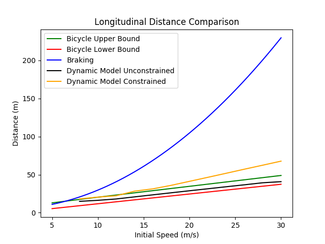
Figure 6: A comparison of the longitudinal distance travelled between swerve and brake manoeuvres, for varying initial velocities. For very low speeds the dynamic model swerves behave poorly and are omitted.

V-B Dynamic Model Validation

Next, we verify that our kinematic approximation is valid by comparing the longitudinal swerve distance under a dynamic model to the distance computed in the preceding sections. We analyze both the cases when the dynamic model is constrained by $a_{\min,\text{brake}}$ and $a_{\min}^{\text{lat}}$, and when it is not. We wish to show that our acceleration constrained bicycle model swerve distances bound the swerve manoeuvre distances of a dynamic model employing both swerving and braking whose accelerations are unconstrained by comfort, but instead constrained by feasibility. We would also like to see at which speeds the constrained kinematic bicycle swerve distance is close to the dynamic model swerve distance when the dynamic model is constrained by comfort. We focus on the ability of the dynamic model to swerve, and not an associated controller, and as a result generate the manoeuvres in open loop. However, doing a grid search over all possible control inputs to find the best swerves is impractical. Instead, we assume that the steering input is broken into 4 equal length intervals of time, and perform binary search over steering rate magnitudes until the boundary conditions in Equation 12 are satisfied. In addition, we also perform linear search over brake input and the total time of the manoeuvre and select the manoeuvre that minimizes the longitudinal swerve distance $x_{c}$. Note that these generated swerves are not optimal for the dynamic model, but are feasible.

The parameters used in our validation are summarized in Table I. We chose $a_{\min,\text{brake}}$ to represent braking at the limit of comfort, and $a_{\max,\text{brake}}$ was chosen to represent a hard, uncomfortable brake. The swerves generated for various initial speeds are illustrated in Figure 7.

TABLE I: Parameters Table

$m$	1239 kg	$l_{f}$	1.19 m	$l_{r}$	1.37 m
$I_{zz}$	1752 $\text{kg}\cdot\text{m}^{2}$	$e_{SP}$	0.5 m	$R$	0.302 m
$c_{w}$	0.3	$\rho_{\text{drag}}$	1.25 $\frac{\text{kg}}{\text{m}^{3}}$	$A$	1.438
$B_{f}$	10.96	$C_{f}$	1.3	$D_{f}$	4560.4
$E_{f}$	-0.5	$B_{r}$	12.67	$C_{r}$	1.3
$D_{r}$	3947.81	$E_{r}$	-0.5	$a_{\max}^{\text{lat}}$	4.0 $\frac{\text{m}}{\text{s}^{2}}$
$a_{\min}^{\text{lat}}$	2.0 $\frac{\text{m}}{\text{s}^{2}}$	$a_{\min,\text{brake}}$	2.0 $\frac{\text{m}}{\text{s}^{2}}$	$\mu$	0.1 m
$a_{\max,\text{accel}}$	2.0 $\frac{\text{m}}{\text{s}^{2}}$	$a_{\max,\text{brake}}$	8.0 $\frac{\text{m}}{\text{s}^{2}}$	$\rho$	0.1 s
$\alpha$	3.7 m	$d_{r}$	2.3 m	$d_{f}$	2.4 m
$b_{r}$	0.9 m	$b_{l}$	0.9 m	$\delta_{\max}$	$\frac{\pi}{6}$

Using these computed swerves, we then compute the lateral clearance distance $y_{c}$ as before and find the longitudinal swerve distance travelled $x_{c}$ that occurs at time $t_{c}$. Substituting this value in at Equations 30 and 36 then gives the required longitudinal safe distance for the dynamic model. For the range of initial vehicle speeds where swerving is more efficient than braking, the longitudinal safe distances required for the dynamic model are plotted and compared to those computed in Section IV in Figure 6.

Figure 7: The swerve manoeuvres generated according to the dynamic model. Each swerve is for a different initial speed in the interval [10, 30] $\frac{\text{m}}{\text{s}}$. The arrows denote the heading of the vehicle.

V-C Simulation Results

In Figure 6, we compare the braking distance and the swerve longitudinal distance travelled when avoiding a stationary object. This plot illustrates the advantage of swerves; for initial rear vehicle speeds greater than 8 $\frac{\text{m}}{\text{s}}$, the swerves reach safety using less longitudinal distance than braking does. We note that as $a_{\min,\text{brake}}$ is increased, the crossover point of velocity where swerves become advantageous increases as well. However, due to the quadratic nature of the braking distance, swerves always eventually become more advantageous at high speeds. From the figure, we can see that when the accelerations of the dynamic model are constrained, the swerve distance of the kinematic model is a reasonable approximation of the dynamic model, with error between 0.7-7.7%, which is reasonable to expect for a kinematic approximation [18]. In the case where the dynamic model is unconstrained by comfort (only by feasibility), the longitudinal swerve distance required is within 15.6-24.0% error of the upper bound distance of the kinematic model, and is completely bracketed by the kinematic upper and lower bounds across a range of speeds from 8-30 $\frac{\text{m}}{\text{s}}$. This shows that our acceleration constrained kinematic approximation can accurately approximate the swerve distance required by the constrained dynamic single-track model up to mid-ranged initial speeds, and can bound the swerve distance required by the unconstrained dynamic model across the entire range of speeds.

In Figure 8, the universal safe following distance required as clearance when using swerves is compared to the braking following distance, as $a_{\min,\text{brake}}$ is varied from 2, 3, and 4 $\frac{\text{m}}{\text{s}^{2}}$. In these plots, all vehicles are moving at an equal speed, displayed on the x-axis. These plots show that as the speeds of the vehicles increase, the following distance decreases when allowing swerve manoeuvres, when compared to braking alone. As $a_{\min,\text{brake}}$ increases, the speeds where swerves become more effective also increases. For increasing $a_{\min,\text{brake}}$ of 2, 3, and 4 $\frac{\text{m}}{\text{s}^{2}}$, these speeds are 8.1, 11.4, and 14.6 $\frac{\text{m}}{\text{s}}$, respectively. The universal following distance is also reduced by up to 42% across all 3 values of $a_{\min,\text{brake}}$ when using swerves as opposed to braking alone.

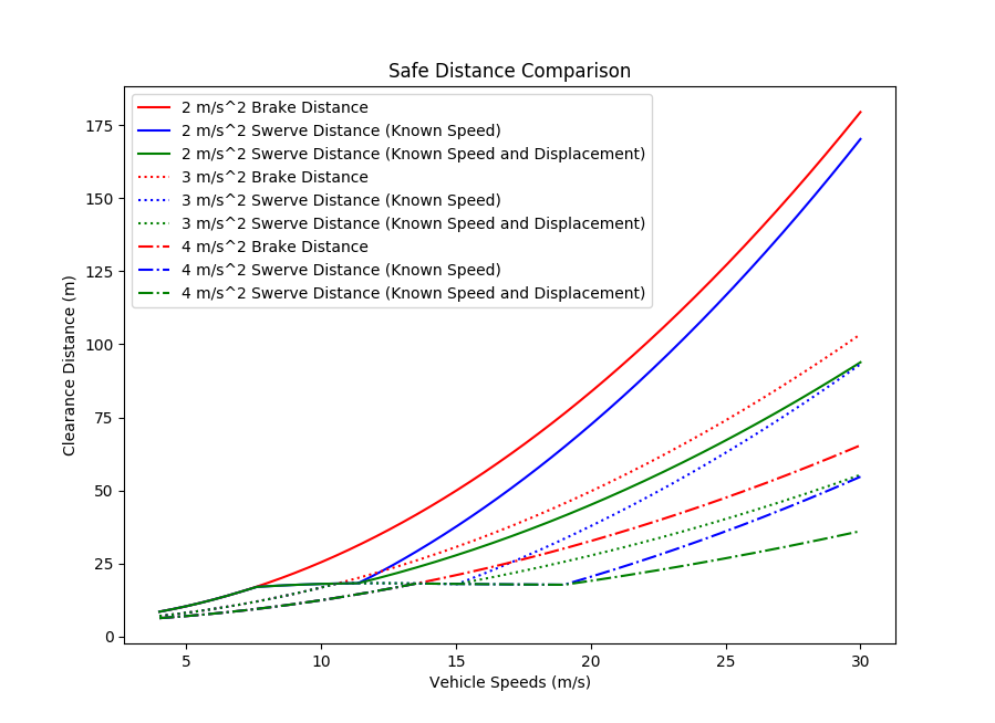
Figure 8: The universal following distance required for safety when $a_{\min,\text{brake}}$ is 2, 3, and 4 $\frac{m}{s^{2}}$.

VI Conclusions

In this work, we outlined a method for extending the RSS framework to include swerve manoeuvres in addition to the standard brake manoeuvre available in the framework. We proved the safety of these manoeuvres under a set of reasonable assumptions about responsible behaviour, while incorporating the original assumptions in the RSS framework. This extended framework results in a significant reduction in following distance at high speeds. In addition, the kinematic model was shown to conservatively bound the longitudinal distance required for swerves executed for the dynamic model.

In future work, we would like to extend the inclusion of swerve manoeuvres to more general cases. One option would be to generalize the swerve manoeuvre to arbitrary Frenet frames, as opposed to straight lines. One could also compute bounds on the error from using a straight line approximation to the Frenet frame. Further experimental work of the RSS framework and its extensions, through on-car testing or scenario simulation, would also be beneficial.

References

- [1] E. Thorn, S. Kimmel, and M. Chaka, “A framework for automated driving system testable cases and scenarios,” Virgina Tech Transportation Institute, Tech. Rep. DOT HS 812 623, Sep 2018. [Online]. Available: https://www.nhtsa.gov/sites/nhtsa.dot.gov/files/documents/13882-automateddrivingsystems˙092618˙v1a˙tag.pdf
- [2] Y. Abeysirigoonawardena, F. Shkurti, and G. Dudek, “Generating adversarial driving scenarios in high-fidelity simulators,” 2019 International Conference on Robotics and Automation (ICRA), 2019.
- [3] M. Althoff, D. Althoff, D. Wollherr, and M. Buss, “Safety verification of autonomous vehicles for coordinated evasive maneuvers,” 2010 IEEE Intelligent Vehicles Symposium, 2010.
- [4] M. Althoff and J. M. Dolan, “Online verification of automated road vehicles using reachability analysis,” IEEE Transactions on Robotics, vol. 30, no. 4, pp. 903–918, 2014.
- [5] S. Shalev-Shwartz, S. Shammah, and A. Shashua, “On a formal model of safe and scalable self-driving cars,” CoRR, vol. abs/1708.06374, 2017. [Online]. Available: http://arxiv.org/abs/1708.06374
- [6] K. Leung, E. Schmerling, M. Chen, J. Talbot, J. C. Gerdes, and M. Pavone, “On infusing reachability-based safety assurance within probabilistic planning frameworks for human-robot vehicle interactions,” 2018 International Symposium on Experimental Robotics, 2018.
- [7] M. Gerdts, “Solving mixed-integer optimal control problems by branch & bound: a case study from automobile test-driving with gear shift,” Optimal Control Applications and Methods, vol. 26, no. 1, pp. 1–18, 2005.
- [8] H. B. Pacejka and E. Bakker, “The magic formula tyre model,” Vehicle System Dynamics, vol. 21, pp. 1–18, 1992. [Online]. Available: https://doi.org/10.1080/00423119208969994
- [9] C. Schmidt, F. Oechsle, and W. Branz, “Research on trajectory planning in emergency situations with multiple objects,” 2006 IEEE Intelligent Transportation Systems Conference, 2006.
- [10] Z. Shiller and S. Sundar, “Optimal emergency maneuvers of automated vehicles,” eScholarship, University of California, Oct 2005. [Online]. Available: https://escholarship.org/uc/item/4xc0k0fs
- [11] ——, “Emergency maneuvers of autonomous vehicles,” IFAC Proceedings Volumes, vol. 29, no. 1, pp. 8089–8094, 1996.
- [12] ——, “Emergency maneuvers for ahs vehicles,” SAE Technical Paper Series, 1995.
- [13] P. Dingle and L. Guzzella, “Optimal emergency maneuvers on highways for passenger vehicles with two- and four-wheel active steering,” Proceedings of the 2010 American Control Conference, 2010.
- [14] Z. Shiller and S. Sundar, “Emergency lane-change maneuvers of autonomous vehicles,” Journal of Dynamic Systems, Measurement, and Control, vol. 120, no. 1, p. 37, 1998.
- [15] H. Jula, E. Kosmatopoulos, and P. Ioannou, “Collision avoidance analysis for lane changing and merging,” IEEE Transactions on Vehicular Technology, vol. 49, no. 6, pp. 2295–2308, 2000.
- [16] C. Pek, P. Zahn, and M. Althoff, “Verifying the safety of lane change maneuvers of self-driving vehicles based on formalized traffic rules,” 2017 IEEE Intelligent Vehicles Symposium (IV), 2017.
- [17] J. Kong, M. Pfeiffer, G. Schildbach, and F. Borrelli, “Kinematic and dynamic vehicle models for autonomous driving control design,” 2015 IEEE Intelligent Vehicles Symposium (IV), 2015.
- [18] P. Polack, F. Altche, B. Dandrea-Novel, and A. D. L. Fortelle, “The kinematic bicycle model: A consistent model for planning feasible trajectories for autonomous vehicles?” IEEE Intelligent Vehicles Symposium, 2017.
- [19] J. M. Snider, “Automatic steering methods for autonomous automobile path tracking,” Master’s thesis, Carnegie Mellon University, 2009.
- [20] A. D. Luca, G. Oriolo, and C. Samson, “Feedback control of a nonholonomic car-like robot,” Lecture Notes in Control and Information Sciences Robot Motion Planning and Control, pp. 171–253, 1998.