ART²: A 3D Parallel Multi-wavelength Radiative Transfer Code for Continuum and Atomic and Molecular Lines

Abstract

ART² is a 3D multi-wavelength Monte Carlo radiative transfer (RT) code that couples continuum and emission lines to track the propagation of photons and their interactions with the ISM. The original ART² has been extensively applied to hydrodynamics simulations to study panchromatic properties of galaxies and ISM. Here, we describe new implementations of non-local thermodynamic equilibrium RT of molecular and atomic fine structure emission lines, and the parallelization of the code using a number of novel methods. The new ART² can efficiently and self-consistently produce a full spectrum that includes both continuum and lines such as [CII], [NII], [OIII], Ly$\alpha$, and CO. These essential features, together with the multi-phase ISM model and the adaptive grid, make ART² a multi-purpose code to study multi-wavelength properties of a wide range of astrophysical systems from planetary disks to large-scale structures.

To demonstrate the capability of the new ART², we applied it to two hydrodynamics simulations: the zoom-in Milky Way Simulation to obtain panchromatic properties of individual galaxies, and the large-scale IllustrisTNG100 Simulation to obtain global properties such as the line intensity mappings. These products are vital for a broad array of studies. By enabling direct comparison between numerical simulations and multi-band observations, ART² provides a crucial theoretical framework for the understanding of existing and future surveys, and the synergy between multi-band galaxy surveys and line intensity mappings. Therefore, ART² is a powerful and versatile tool to bridge the gap between theories and observations of cosmic structures.

1 Introduction

The past decade has witnessed a “golden age" of panchromatic astronomy thanks to an impressive array of multi-wavelength instruments, from NASA’s Great Observatories (Hubble, Chandra, and Spitzer), to small-scale missions such as GALEX, SWIFT, FERMI, and NuSTAR, to European missions such as Herschel, Planck, XMM, and to ground-based telescopes as SDSS, Subaru and ALMA (e.g., see a recent review by Megeath et al. 2019). These observatories span the full electromagnetic spectrum from radio, to infrared /optical /UV, and to X-ray and gamma-ray. These facilities have led to major discoveries in observational cosmology from multi-band surveys using both continuum and emission lines. These surveys have measured the cosmic star formation history (e.g., Madau & Dickinson, 2014; Goto et al., 2019; Wilkins et al., 2019), the black hole growth history (e.g., Hickox & Alexander, 2018; Aird et al., 2019), the evolution of galaxy luminosity functions (e.g., Bouwens et al., 2014; Koprowski et al., 2017; Park et al., 2019), the evolution of interstellar medium (ISM) (e.g., Scoville et al., 2017; Decarli et al., 2018; Riechers et al., 2019), and a full-spectrum extragalactic background light (e.g., Hill et al., 2018).

In recent years, a new technique called Line Intensity Mapping (LIM) has emerged as a promising method to study the evolution of the Universe (e.g., Lidz et al., 2011; Visbal et al., 2011; Pullen et al., 2014; Kovetz et al., 2017; Fonseca et al., 2017; Moradinezhad Dizgah & Keating, 2019; Karkare & Bird, 2018; Chung et al., 2019; Sun et al., 2019; Bernal et al., 2019). In contrast to the aforementioned single-object telescopes which require high resolutions, the LIM technique uses low-resolution instruments to measure the integrated emission of atomic and molecular lines from galaxies and the intergalactic medium (IGM) such as Ly$\alpha$, [CII], CO and 21-cm line. This technique can probe a wide array of topics such as the epoch of reionization, cosmic star formation history, and evolution of ISM and IGM.

Looking ahead, the next decade will be a new era in astrophysics with a host of planned or proposed ambitious facilities from radio to x-ray, such as SKA, JWST, WFIRST, LSST, Athena and Lynx, and LIM instruments such as CONCERTO, SPHEREx and Origins (e.g., see recent reviews by Cooray et al. 2019 and Kovetz et al. 2019). These developments suggest that full-spectrum surveys that include both continuum and lines will be the name of the game, and that a synergy between galaxy surveys and LIMs is on the horizon to provide a complete picture of our cosmos.

However, in order to understand the existing observations and the underlying physical processes, and prepare for the future surveys, we need a comprehensive theoretical framework that can simultaneously provide both the physical and the panchromatic properties of galaxies, active galactic nuclei, ISM and IGM across cosmic time. A desired approach is to combine state-of-the-art cosmological simulations with state-of-the-art multi-wavelength radiative transfer calculations. Radiation at different wavelengths are often intertwined due to the interaction between photons and baryonic matter in different forms, such as ionized gas, molecular clouds, and dusts. Therefore, detailed comparison of observations and theoretical models must include radiative transfer calculations that couples photons of different wavelengths and the physical states of matter (e.g., Steinacker et al., 2013; Kewley et al., 2019).

Recently, a number of impressive cosmological simulations have been performed, including large-scale ones Illustris (precursor of IllustrisTNG, Vogelsberger et al., 2014; Genel et al., 2014), EAGLE (Schaye et al., 2015; Crain et al., 2015), Horizon-AGN (Dubois et al., 2014), Romulus (Tremmel et al., 2017), Simba (Davé et al., 2019), Magneticum (Dolag et al., 2016), and IllustrisTNG (Pillepich et al., 2018a; Springel et al., 2018; Marinacci et al., 2018; Naiman et al., 2018; Nelson et al., 2018, 2019a, 2019b; Pillepich et al., 2019), as well as high-redshift simulations such as BlueTides (Feng et al., 2016) and Sphinx (Rosdahl et al., 2018), and zoom-in ones such as MilkyWay (Zhu & Li, 2016), FIRE-2 (Hopkins et al., 2018), and Auriga (Grand et al., 2017).

On the other hand, a number of radiative transfer codes have been developed in recent years, for examples, RADMC-3D Dullemond et al. (2012) and SKIRT (Camps & Baes, 2015) for dust continuum; CLOUDY (Ferland et al., 2017), DESPOTIC (Krumholz, 2014), LIME (Brinch & Hogerheijde, 2010), MAIHEM (Gray et al., 2015) and MAPPINGS (Allen et al., 2008) for emission lines from ionized ISM; MOLLIE (Keto & Rybicki, 2010) and Turtlebeach (Narayanan et al., 2009) for molecular lines, CRASH for ionization (Hariharan et al., 2017), as well as IGMtransfer (Laursen, 2011), McLya (Schaerer et al., 2011) and RASCAS (Michel-Dansac et al., in prep) for Ly$\alpha$ line and other calculations  (e.g., Zheng et al., 2010, 2011; Dijkstra et al., 2016).

Over the last decade, we have developed a 3D Monte Carlo radiative transfer code, All-Wavelength Radiative Transfer with Adaptive Refinement Tree (ART²). ART² originally included continuum transfer of dust scattering and absorption, which produced a continuum spanning 7 orders of magnitude in wavelength from X-ray to sub-millimeter. The code was first used to model broad-band properties of high-redshift quasars (Li et al., 2008). The ionization of neutral Hydrogen, and resonant scattering of Ly$\alpha$ photons were later added as additional modules (Yajima et al., 2012a). This version of ART² has been extensively applied to multi-scale cosmological hydrodynamic simulations to study multi-band properties of galaxies and quasars, such as the 21-cm signals of the first galaxies and quasars, high-redshift Ly$\alpha$ emitters, and progenitors of the Milky Way (Yajima et al., 2012c, 2013; Yajima & Li, 2014; Yajima et al., 2015, 2018; Arata et al., 2019, 2020).

In the present paper, we further extend the scope of ART² to make it more versatile, by improving the algorithms of existing modules, increasing its efficiency by parallelization, and adding new modules for the non-local thermal equilibrium (non-LTE) molecular and atomic fine structure line transfer process, in order to provide a comprehensive framework for both continuum and useful lines such as Ly$\alpha$, [CII], [NII], [OIII], and CO as commonly employed in multi-wavelength surveys of galaxies and ISM.

The paper is organized in three parts: the code, the applications, and the conclusions. In Section 2, we describe the improvements to the original ART², and new implementations of the non-LTE molecular and atomic line transfer processes, their verifications and the parallelization in the following order: dust continuum in Section 2.1; the Hydrogen ionization and Ly$\alpha$ resonant line transfer in Section 2.2; the non-LTE molecular line transfer in Section 2.3; the non-LTE atomic fine structure line transfer in Section 2.4; and method for RT through a sub-grid multi-phase interstellar medium model in Section 2.5. In Sections 3, we demonstrate the power of the new ART² by applying it to two hydrodynamics simulations: the zoom-in Milky Way Simulation to obtain multi-band properties of individual galaxies in Sections 3.1, and the large-scale IllustrisTNG100 Simulation to obtain global properties of the entire system such as the line intensity mappings in Sections 3.2. Finally, in Section 4 we discuss and summarize the essential features of ART² and its potential contributions to astrophysics.

2 ART²: The State-of-the-art Radiative Transfer Code for Continuum and Lines

ART² is a 3D, fully-parallel, multi-wavelength Monte Carlo RT code that can self-consistently and efficiently calculate a full spectrum that includes a continuum from X-ray to sub-millimeter, atomic lines such as Ly$\alpha$, [CII], [NII] and [OIII], and molecular lines such as CO and HCN. In addition, ART² adopts a multi-phase ISM model, which ensures an appropriate prescription of the ISM physics in case hydrodynamics simulations have insufficient resolution to resolve the multi-phase ISM, and it employs an adaptive grid scheme, which can handle arbitrary geometry and cover a large dynamical range of gas densities in hydrodynamical simulations. These essential features make ART² a flexible, reliable and versatile tool to study the multi-wavelength properties of a wide range of astrophysical systems, from planetary disks, to star forming regions, to galaxies, and to large-scale structures of the Universe.

ART² was first developed with continuum only to study the dust properties of high-redshift quasars (Li et al., 2008). Since then, significant developments and improvements have been made to it over the years. We added modules of ionization of neutral hydrogen and ${\rm Ly}\alpha$ emission in Yajima et al. (2012b), and recently we have implemented the non-LTE radiative transfer of molecular and atomic fine structure lines, and have parallelized all the RT processes.

The main objective of ART² is to seek the solution of the radiative transfer equation (Rybicki & Lightman, 1986):

$$\\ \frac{dI_{\nu}}{ds}=-\alpha_{\nu}I_{\nu}+j_{\nu},$$ (1)

or equivalently,

$$\\ \frac{dI_{\nu}}{d\tau_{\nu}}=-I_{\nu}+S_{\nu},$$ (2)

where $I_{\nu}$ is the specific intensity of the radiation, $\alpha_{\nu}$ is the total opacity, $j_{\nu}$ is the emissivity, $\tau_{\nu}=\alpha_{\nu}ds$ is the differential optical depth, and $S_{\nu}=j_{\nu}/\alpha_{\nu}$ is the source function.

This is a multi-dimensional equation as the radiation depends on the positions $(x,y,z)$, the viewing angles $(\Theta,\Phi)$, the photon frequency $(\nu)$, and in some cases also the time $(t)$. To solve such a complex problem, ART² uses the flexible Monte Carlo method to robustly follow the propagation of the photons and their interactions with ISM and IGM with rigorous random samplings, as described in Li et al. (2008).

The type of radiative transfer problem is prescribed by specific coupling between the $S_{\nu}$ and the local state of the matter responsible for absorption, scattering, and emission. In the case of dust continuum transfer, the emissivity function depends on the dust temperature, which in turn is determined by the local radiative field through the radiative equilibrium. For the transfer of ionizing radiation, the opacity function depends on the thermal and ionization state of various atomic species, which must be determined through the thermal and ionization equilibrium involving the radiation field through photoionization. For the transfer of molecular or atomic lines, the source function depends on the statistical populations of molecular or atomic levels, which are also coupled with the radiation field through photo-excitation. The ${\rm Ly}\alpha$ resonance scattering is the only process in which the radiation is not explicitly coupled with the matter state. However, ${\rm Ly}\alpha$ scattering presents its own unique challenges due to the often extremely large scattering optical depth.

In the following sections, we describe the numerical techniques implemented in ART² for these specific problems. In particular, we highlight the new improvements over the original implementations, and the novel approaches for the non-LTE radiative transfer of molecular and atomic fine structure lines, and the parallelization of each RT process.

2.1 Dust Continuum Radiative Transfer

The dust RT implemented in the original ART² is based on the algorithm of Bjorkman & Wood (2001), which exploits the fact that the dust opacity does not depend on its temperature, and obtains the solution of radiative equilibrium and emergent spectrum simultaneously without iterations. The central ingredient of this algorithm is the immediate re-emission of the photon packet by the dust following an absorption event. For each absorption and re-emission step, the radiative equilibrium is maintained by updating the dust temperature so that the re-emitted luminosity is the same as the absorbed one, while the re-emitted photon frequency is sampled from a spectrum proportional to:

$$\\ \Delta j_{\nu}=\kappa_{\nu}\rho\left[B_{\nu}(T_{i})-B_{\nu}(T_{i-1})\right],$$ (3)

where $\kappa_{\nu}$ is the dust opacity, $\rho$ is the gas density of the cell where the photon is absorbed, $B_{\nu}$ is the Planck function, and $T_{i}$ is the dust temperature after the absorption of the $i$-th photon packet while maintaining the radiative equilibrium.

After all photons have been traced, it is evident that the ensemble of all re-emitted photons are sampled from the spectrum $\kappa_{\nu}\rho B_{\nu}(T_{d})$, where $T_{d}$ is the final dust temperature in radiative equilibrium.

While this algorithm is very efficient, it has two drawbacks. First, all photon packets are completely destroyed and re-emitted in cells where the absorptions occur. This leads to large statistical sampling errors. Second, the immediate re-emission step with temperature update leads to dependency of successively traced photons, making it difficult to parallelize the algorithm. In the present work, we implement a modified version of this algorithm that avoids these two problems while retaining its non-iterative nature.

Instead of absorbing and re-emitting the photon packets completely at a single site, we first trace all photon packets without re-emission and dust temperature update. The photon packets are not absorbed statistically in any single cell. Instead we record the average absorbed luminosity along the photon path for the entire batch of photons. Dust scattering, however, is still followed statistically at every interaction site at the time of the scattering, because it would be rather difficult to re-emit the scattered luminosity at a later time or after all the interactions, if the scattering phase function is not isotropic, as is often the case with dust.

After tracing all photon packets, we then update the dust temperature according the total absorbed luminosity at each cell, and re-emit them with a spectrum corresponding to $\kappa_{\nu}\rho B_{\nu}(T_{0})$. The re-emitted thermal photons are then traced again, whose absorption results in further update of the dust temperature to $T_{1}$. The absorption and re-emission processes are then repeated until the total absorbed luminosity becomes negligible. Denoting the dust temperature after the $i$-th step as $T_{i}$, the frequencies of the re-emitted photons in each step are sampled from the spectrum of Equation 3.

After convergence, we obtain both the radiative equilibrium solution and the emergent spectrum as in the original algorithm. However, in this modified method, the photon packets traced in each step are uncorrelated. It is therefore straightforward to distribute the ray tracing workload over a large number of processors. Data communication is only required for updating the dust temperature, where the total absorbed luminosity is collected from individual processors.

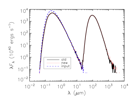
Figure 1: Test of the new dust continuum algorithm with a disk galaxy model. The emergent continuum from the disk galaxy is calculated using the new and the old (Li et al., 2008) algorithms. The spectra produced by both algorithms are nearly identical.

To test this new algorithm and the parallelization, we run the same test problem of dust radiative transfer through a model disk as in Li et al. (2008). A comparison of the emergent spectrum from the new algorithm with that from the original one is shown in Figure 1. The reprocessed spectra from the two implementations are virtually indistinguishable, except at frequencies where statistical sampling error becomes dominant, thus verifying the new algorithm for dust continuum RT and the parallelization.

2.2 Ionization and Ly$\alpha$ Scattering

The ionization and Ly$\alpha$ scattering components implemented in ART² were described in detail in Yajima et al. (2012a). In this Section, we only describe the improvements to the original implementation in the new ART².

Similar to the continuum dust transfer, we modified the implementation of the ionization process, by not treating absorption as a single statistical event, but by following the average absorbed luminosity along the paths of photon packets. However, there is an important distinction between the dust and the ionization RT. Due to the tight coupling between the gas absorption opacity and its ionization fraction, one must update the ionization states of the gas cell as the photons pass through it. This creates dependency in successively traced photons, making parallelization difficult.

To circumvent this issue, we have developed a two-step procedure to evolve the gas ionization fraction. In the first step, individual photon packets are traced, and the ionization states are updated as the ray tracing proceeds. When multiple, e.g., $n_{p}$, processors are used for this step, each processor works independently by tracing an equal number of photons to advance the ionization evolution for a reasonable time step, $\delta t$. This provides $n_{p}$ independent estimates of the ionizing flux within each cell. In the second step, these independent estimates are collected and averaged to provide a single improved estimate, which is then used to evolve the ionization states for the same time step. This two-step process is then repeated to advance the ionization state evolution until convergence is reached.

In some situations, one can ignore the time evolution of the ionization states but only needs the final equilibrium. For this purpose we implement another mode to solve the equilibrium ionization fractions iteratively. In each iteration, the ray tracing procedure is similar to that used in advancing the ionization evolution for one time step. When an estimate of the ionizing flux is available from the ray tracing step, we solve the steady state statistical equilibrium equation, instead of evolving the ionization fractions at this time step.

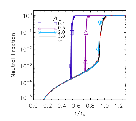
Figure 2: Test of the new ionization algorithm with a dust free Strömgren sphere. The neutral H fraction profile of a dust free Strömgren sphere is calculated at different times. The profile at $t/t_{\rm rec}=3$ successfully converges to the final solution obtained with the equilibrium ionization mode, as shown in red curve.

We test the new implementation of the ionization process with a dust-free Strömgren sphere model at a temperature of $10^{4}$ K. We calculate the neutral H fraction profile at different times relative to the recombination time scale, as shown in Figure 2. The ionization front reaches the Stroömgren sphere radius at $t/t_{\rm rec}=3$, and the neutral fraction profile successfully converges to the final solution obtained with the equilibrium ionization mode as expected.

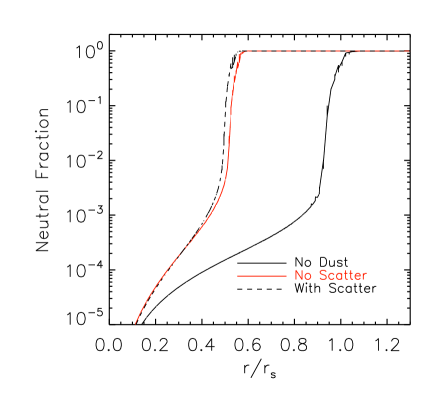
Figure 3: A comparison of dust-free and dusty Strömgren sphere calculated with the equilibrium ionization mode. A dusty sphere has a smaller ionization radius than a dust-free one due to dust absorption and scattering of the ionizing photons.

We also compare the equilibrium neutral fraction profiles of a dust-free and a dusty Strömgren sphere calculated with the equilibrium ionization mode, as shown in Figure 3.The dusty sphere has an absorption optical depth of 4.0 at the Stroömgren sphere radius. The location of the ionization front for the dusty sphere agrees with the analytic solution of Spitzer (1978). Figure 3 shows that dusty sphere has a smaller ionization radius than dust-free medium due to absorption of the ionizing photons by dust, and that dust scattering has a small effect on the equilibrium neutral fraction profile and shrinks the ionized sphere.

Figure 4: Test of the new Ly$\alpha$ algorithm with a dusty slab. The escape fraction of Ly$\alpha$ photons from a source at the center of a dusty slab is calculated at different absorption optical depths. The parameter $\rm{(a\tau_{0})^{1/3}\tau_{abs}}$ is a scaled optical depth combining the optical depth at the line center $\tau_{0}$ and the total absorption optical depth $\tau_{\rm abs}$, as defined in Neufeld (1990). Our result agrees with the analytic solution of Neufeld (1990) very well.

The algorithm for the resonant scattering of Ly$\alpha$ photons is the same as that described in Yajima et al. (2012a), with one improvement for the handling of dust absorption. Similar to the implementations of the dust continuum and ionization RT, the dust absorption is followed as the average luminosity of the entire batch of photons gradually diminishing along the photon path, instead of a single statistical event that destroys the entire photon. Figure 4 shows the standard Neufeld (Neufeld, 1990) test for the escape fraction of Ly$\alpha$ photons from a source placed at the center of a dusty slab. The comparison demonstrates good agreement between our new Ly$\alpha$ calculation and the analytic solution.

2.3 Molecular Line Radiative Transfer

The excitation of many molecules is non-LTE because the gas density is usually below the high threshold required for local thermal equilibrium. The line transfer is further complicated by the closely coupled relation between source function, level population and radiation field. Our implementation of the non-LTE molecular line transfer in ART² is based on the accelerated Monte Carlo (AMC) method of Hogerheijde & van der Tak (2000b), and the implementation of the AMC method on a 3D adaptive grid is similar to that of Rundle et al. (2010). Here we give a brief description of the methods and highlight the improvements we made in ART².

The basic problem in non-LTE molecular line transfer is to seek the solution of the coupled equations of statistical equilibrium of level populations $n_{i}$ and radiative transfer,

$$\\ \sum^{N}_{j\neq{i}}{n_{j}P_{ji}}-n_{i}\sum^{N}_{j\neq{i}}{P_{ij}}=0,$$ (4)

where the coefficients $P_{ij}$ are given by:

$$\\ P_{ij}=\left\{\begin{array}[]{l l}A_{ij}+B_{ij}\bar{J}_{\nu}+C_{ij}&\quad(i>j)\\ B_{ij}\bar{J}_{\nu}+C_{ij}&\quad(i<j)\\ \end{array}\right.$$ (5)

where $A_{ij}$ and $B_{ij}$ are Einstein coefficients for transition from level i to j, and $C_{ij}$ are calculated as:

$$\\ C_{ij}=n_{col}K_{ij}$$ (6)

where $n_{col}$ is the number density of collision partner, which is often taken to be molecular hydrogen $\rm{H_{2}}$, and $K_{ij}$ are the collisional rate coefficients in unit of $\rm{cm^{3}~{}s^{-1}}$.

The coupling to the radiation comes from the frequency integrated mean intensity for a given transition $\bar{J}_{\nu}$,

$$\\ \bar{J}_{\nu}=\int J_{\nu}\phi_{\nu}{d\nu}=\frac{1}{4\pi}\int{I_{\nu}\phi_{\nu}{d\nu}{d\Omega}},$$ (7)

where $I_{\nu}$ is the specific intensity of the radiation field, and $\phi_{\nu}$ is the normalized line profile.

In AMC, the Monte Carlo ray tracing used to obtain $\bar{J}_{\nu}$ takes a cell-centered point of view. A discrete set of rays passing through each cell with different angles and frequencies are sampled to give an estimate of the double integral,

$$\bar{J}_{\nu} = \bar{J}_{\nu}^{ext}+\bar{J}_{\nu}^{int}$$ (8)

$$= \frac{\sum_{i}{[I^{i}_{\nu}{e^{-\tau_{i}}}+S^{i}_{\nu}(1-e^{-\tau_{i}})]\phi_{\nu}}}{\sum_{i}{\phi_{\nu}}},$$

where the index $i$ denotes the $i$-th ray in the sample.

In the original AMC method, the frequencies are uniformly sampled around the local systematic velocity vector. $I^{i}_{\nu}$ is the incident radiation on the edge of cell for $i$-th ray, which is obtained by integrating the radiative transfer equation from the cell edge to infinity. $S^{i}_{\nu}$ is the source function in the cell. $\tau_{i}$ corresponds to the distance $ds_{i}$ between the spot where the ray contributes to the cell and the point where the ray intersects the boundary of the cell. The convenient split of $\bar{J}_{\nu}$ into the external part, $\bar{J}_{\nu}^{ext}$, and the internal part, $\bar{J}_{\nu}^{int}$, is the key to the acceleration scheme used in AMC. In each iteration to solve Equation 4, an inner iteration is inserted to obtain the level populations of the local cell while fixing $\bar{J}_{\nu}^{ext}$. The benefit of this inner iteration is substantial when the optical depth of the local cell is relatively large.

In the ART² implementation, we make two modifications to Equation 8. First, the frequencies are not randomly sampled, instead, we estimate the integration over $\nu$ by a five-point Gauss quadrature formula. This is uniquely suitable as the line profile is often close to Gaussian function. Second, the external and internal contributions to mean intensity are taken to be the average along the photon path within the cell, instead of the value at a random point. Equation 8 may be rewritten as,

$$\\ \bar{J}_{\nu}=\Sigma_{ik}w_{k}\phi_{k}\left[\beta_{ik}I^{ik}+(1-\beta_{ik})S^{ik}\right],$$ (9)

where the additional index $k$ denotes the Gauss quadrature points in the frequency space, $w_{k}$ are the quadrature weights, and $\beta_{ik}$ is an escape probability given by,

$$\\ \beta_{ik}=\frac{1-e^{-\tau_{ik}}}{\tau_{ik}},$$ (10)

where $\tau_{ik}$ is the total optical depth of the $i$-th ray at $k$-th frequency within the local cell.

This recasts $\bar{J}_{\nu}$ into a familiar form encountered in, e.g., the escape probability formalism, or the large velocity gradient (LVG) approximation (de Jong et al., 1975; Goldreich & Kwan, 1974). The source function $S^{ik}$ generally includes contributions from the molecular line and dust. The line contribution depends on the level populations, which may make the inner iteration unstable if the cell optical depth is large enough so that the internal part of the mean intensity dominates, or equivalently, if $\beta_{ik}$ is very small. In such cases, it is more convenient to rewrite the source function $S^{ik}$ in Equation 9 to include the line source function $S^{0}_{ul}$ and a residual term $S^{ik}_{\rm res}$:

$$S^{ik} = (S^{ik}-S^{0}_{ul})+S^{0}_{ul}=S^{ik}_{\rm res}+S^{0}_{ul}$$

$$S^{0}_{ul} = \frac{2h\nu_{ul}^{3}}{c^{2}}\left[\frac{n_{l}g_{u}}{n_{u}g_{l}}-1\right],$$ (11)

where $S^{0}_{ul}$ is the line source function for transition from $u$ to $l$, which depends on the level populations $n$ and the statistical weight $g$ of level $u$ and $l$, respectively.

As in the LVG approximation, we can drop the $S^{0}_{ul}$ term in the mean intensity, and substitute $S^{ik}$ in Equation 9 with $S^{ik}_{\rm res}$. As suggested in Goldreich & Kwan (1974), the combined effect of dropping $S^{0}_{ul}$ on the level population equation is equivalent to modifying the Einstein coefficients $A_{ul}$ to $\Sigma_{ik}\beta_{ik}w_{k}\phi_{k}A_{ul}$ in Equation 5. Now the inner iteration to solve the level populations is much more stable when Equation 4 is recast in this form. Note that since the molecular and the atomic fine structure lines we consider here do not have severe population inversion such as strong masing, so a simplified approach of limiting the negative optical depth can be used to solve the statistical equilibrium equations and obtain level population convergence. Once the level population $n$ and $S^{ik}_{\rm res}$ are solved, we can obtain the source function $\beta_{ik}$, and then solve the general radiative transfer equation.

Finally, the improved AMC method implemented in ART² is parallelized by distributing the level population equation for individual cells to different processors. The solutions for individual cells are essentially independent if only the results from the previous iteration is used. Data communication is therefore only needed at the end of iteration to synchronize the level population solutions on the entire grid cross different processors. For the construction of images and spectra, the parallelization is achieved by distributing ray tracing to different processors.

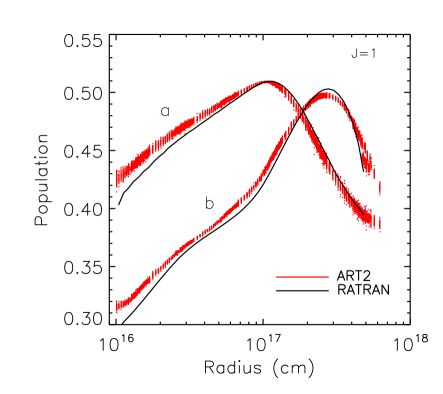
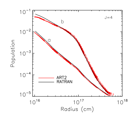
Figure 5: Test of the AMC implementation in ART² with a collapsing cloud model for HCO+ molecule for optically thin (a) and thick (b) cases, in comparison with Ratran. The top panel shows the relative population for $\rm J=1$ level, while the bottom panel shows the same but for $\rm J=4$ level, respectively. The comparisons show good agreement between ART² and Ratran.

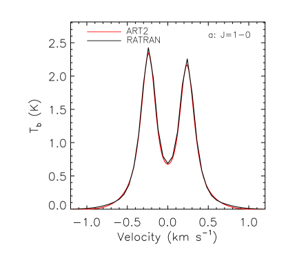
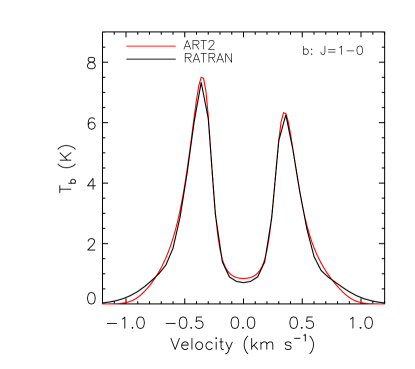
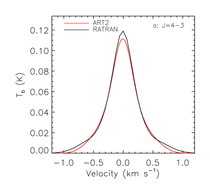
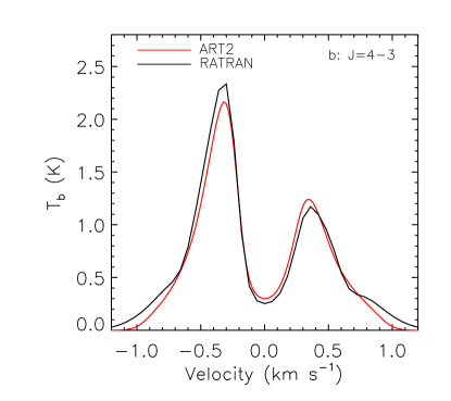
Figure 6: Test of the new molecular RT algorithm in ART² with a collapsing cloud model for HCO+ molecule for optically thin (a) and thick (b) cases, in comparison with Ratran. The top panels show the brightness temperature profiles for $\rm J=1-0$ transition, while the bottom panels show the same but for $\rm J=4-3$. The comparisons show good agreement between ART² and Ratran.

To verify our implementation of the AMC method, we run the test problem of a collapsing cloud for ${\rm HCO}^{+}$ molecule, as presented in van Zadelhoff et al. (2002), with ART² for both optically thin (a) and optical thick (b) cases. We have also run the same models using the one-dimensional code Ratran (Hogerheijde & van der Tak, 2000a), which implements the original AMC method (Hogerheijde & van der Tak, 2000b). The resulting relative populations for the $\rm J=1$ and $\rm J=4$ levels from ART² are shown in Figures 5, in comparisons with results from Ratran. These comparisons show good agreement between ART² and Ratran.

The resulting brightness temperature profiles for $\rm J=1-0$ and $4-3$ transitions are shown in Figures 6, which again show reasonable agreements between ART² and Ratran.

2.4 Atomic Fine Structure Line Transfer

The non-LTE atomic fine structure line transfer includes two steps: First, we solve the ionization equilibrium of individual atomic species and the thermal equilibrium of the gas. After that, we solve the coupled equations of statistical equilibrium of level populations and radiative transfer of fine structure emission lines of individual ionic species using the same method of the molecular line RT in Section 2.3.

In order to treat the fine structure emission lines from atomic ions, the ionization module is extended to include elements other than H. The ionization equilibrium of individual atomic species and the thermal equilibrium of the gas are determined by solving a set of non-linear equations,

$$(C^{a}_{i}+R^{a}_{i})n^{a}_{i} = C^{a}_{i-1}n^{a}_{i-1}+R^{a}_{i+1}n^{a}_{i+1}$$

$$n_{e} = \sum_{a,i}n^{a}_{i}q_{i}$$

$$n^{a} = \sum_{i}n^{a}_{i}$$

$$C(n_{e},T) = H(n_{e},T)$$ (12)

where $n^{a}_{i}$ represents the number density of the charge state $i$ of atomic species $a$; $n^{a}$ is the total density of the atomic species $a$; $n_{e}$ is the electron density; $C^{a}_{i}$ and $R^{a}_{i}$ are the total ionization and recombination rates of the ion, $q_{i}$ is the ion charge; $C(n_{e},T)$ and $H(n_{e},T)$ are the total cooling and heating rates, respectively.

The ionization processes include both photoionization and collisional ionization by electrons, and the recombination processes include both radiative and dielectronic recombinations. Charge exchange reactions between ions and neutral H and He are also included in the ionization and recombination processes. The ionization and recombination rate coefficients of relevant ions needed to compute the ionization equilibrium are taken from the photoionization code CLOUDY version 17.00 (Ferland et al., 2017), while the local ionizing photon flux are determined in our Monte Carlo ray tracing procedure. The cooling and heating rates are also calculated self consistently. The heating sources include photoionization and Compton scattering with high energy photons. The cooling sources include Bremsstrahlung, collisional ionization, radiate and dielectronic recombination, collisional excitation of fine structure lines, and Comptonization with the low energy photons, including cosmic microwave background.

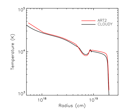
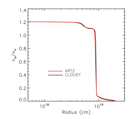
Figure 7: Test of the new atomic fine structure line RT in ART² with a spherical cloud. The radial profile of the gas temperature (top) and the electron density relative to the H atoms (bottom) calculated by ART² are in good agreements with CLOUDY.

Figure 8: A comparison of the HI fraction of a spherical cloud model calculated with ART² and CLOUDY.

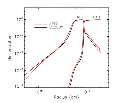
Figure 9: A comparison of the HeI and HeII fractions of a spherical cloud model calculated with ART² and CLOUDY.

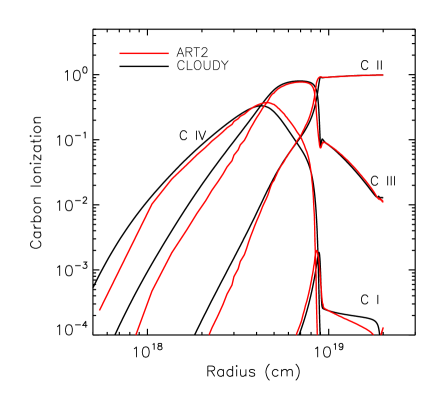
Figure 10: A comparison of the CI – CIV fractions of a spherical cloud model calculated with ART² and CLOUDY.

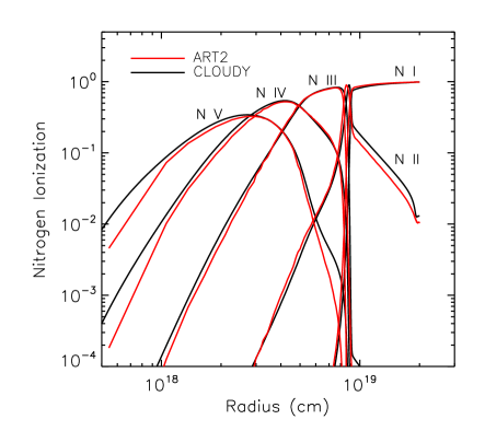
Figure 11: A comparison of the NI – NV fractions of a spherical cloud model calculated with ART² and CLOUDY.

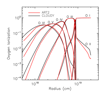
Figure 12: A comparison of the OI – OVI fractions of a spherical cloud model calculated with ART² and CLOUDY.

Figure 13: A comparison of the atomic fine structure line luminosity calculated with ART² and CLOUDY, for the [CII], [NII], [OI] and [OIII] lines. The comparison shows reasonable agreement between ART² and CLOUDY to within 10%.

After the ionization and thermal equilibrium are solved, the radiative transfer of fine structure emission lines of individual ionic species are calculated using the same method as the molecular line RT in Section 2.3. We use the same equations (1) - (9) in Section 2.3, but instead of solving the populations of molecular rotational levels, the fine structure level populations of a given ion are solved. The excitation mechanisms of the atomic lines also differ significantly from those for molecular lines. Collisional excitation with electrons and protons are typically the dominant processes populating the fine structure levels in atomic ions. In our implementation, we include excitations by electron, proton, and neutral H atom. The rate coefficients of collisional processes, transition energies, and spontaneous transition rates are taken from the CLOUDY database.

To verify our implementation, we compare calculations by ART² of a spherical cloud model with a central ionizing source with those by the 1D photoionization code CLOUDY. The gas sphere has a uniform hydrogen density of 100 cm^-3, and a radius of $2\times 10^{19}$ cm, which is about twice the Strömgren radius of the cloud at the temperature of $10^{4}$ K. The ionizing spectrum is a power law with index of 1.5 in the energy range between 10 and 1000 Rydberg, and the total photon rate is $10^{49}$ s^-1. The atomic species included in the calculation are all ions of H, He, C, N, and O. The relative elemental abundances are set at the solar values.

We first calculate the ionization and thermal structures of the cloud, and then the atomic fine structure lines of all species in the gas sphere, with both ART² and CLOUDY. Figure 7 shows the gas temperature and the electron density as a function of radius as calculated by the two codes, and Figures 8 to 12 show the comparisons of the ionization fractions of H, He, C, N, and O computed, respectively. These comparisons show that the thermal and ionization structures calculated by the non-LTE atomic line RT in our 3D ART² are consistent with the 1D calculations by CLOUDY.

Finally, we compute the radiative transfer for the prominent fine structure [CII] line at 158 $\mu$m, the [NII] lines at 122 and 205 $\mu$m, the [OI] lines at 63 and 145 $\mu$m, and the [OIII] lines at 52 and 88 $\mu$m. In Figure 13, we compare the total line luminosities calculated with ART² and CLOUDY. It shows that the luminosities calculated with the two codes agree with each other to within 10% for the 7 strongest lines.

2.5 Radiative Transfer Through a Sub-grid Multi-phase ISM Model

The RT processes in ART² described in previous sections are comprehensive and applicable to situations with vastly different physical scales, such as planetary disks, star forming regions, galaxies and large-scale structures. However, numerical simulations in the cosmological context usually have limited spatial resolution to resolve molecular clouds where stars form. These simulations often employ sub-grid recipes to capture the essence of star formation physics. For example, the Smoothed Particle Hydrodynamics (SPH) code Gadget  (Springel, 2005) implements a sub-grid multi-phase ISM model to describe the star formation processes (Springel & Hernquist, 2003). When post processing such simulations with RT codes, it is important that a consistent sub-grid multi-phase ISM model is followed.

The propagation of photons through a multi-phase ISM was first considered by Neufeld (1991), who calculated the escape of Ly$\alpha$ photons from a clumpy, dusty ISM by modeling the medium as a collection of spherical clouds, which were treated as large particles capable of scattering or absorbing photons. Subsequently, Hobson & Padman (1993) named this approach the “Mega-grain approximation", and they found good agreement between the approximation and calculations using Markov processes. Recently, the “Mega-grain approximation" was adopted by Hansen & Oh (2006) to calculate the Ly$\alpha$ RT using a Monte Carlo method. We use the same approximation and follow the approach of Hansen & Oh (2006) in our treatment of the multi-phase ISM.

In the original ART², we implemented the multi-phase RT for dust continuum transfer by assuming that the cold phase consists of randomly distributed molecular clouds with a given mass-radius relation and a power-law mass distribution function, and statistically sample these clouds in the ray tracing process (Li et al., 2008). The physical properties such as density and volume filling factor of the cold phase were derived from the Gadgetsimulation output. It was shown in that work that the existence of hot and cold dust components are essential to reproduce both near and far infrared observations of high redshift quasars. In the present work, we adopt a similar approach with some modifications to accommodate the new absorption handling and extend it to the RT components other than the dust continuum.

First, to simplify the handling, we do not impose a specific power-law mass distribution function in a single cell like in the original implementation. Instead, all clouds are assumed to have the same mass, $M_{c}$, and radius, $R_{c}$, within a single cell that satisfy the mass-radius relation of the form $M_{c}=AR_{c}^{\alpha}$, where $\alpha$ has a value between 2 and 2.5, as most observations suggest. In principle, the normalization $A$ could vary from galaxy to galaxy, but a value of a few hundred is appropriate for galaxies like Milky Way (Solomon et al., 1987). When a photon passes through a cell that contains cold clouds, the total opacity is given by:

$$\\ \alpha^{t}=(1-f_{v})\alpha^{t}_{h}+f_{v}\beta_{c}\alpha^{t}_{c},$$ (13)

where $f_{v}$ is the volume filling factor of the cold phase in the cell, the index $t$ is either $s$ for scattering and $a$ for absorption, while $\alpha^{t}_{h}$ and $\alpha^{t}_{c}$ are the respective opacities of hot and cold phases, and $\beta_{c}$ is the escape probability of individual cold clouds, which we model as

$$\\ \beta_{c}=\frac{1-e^{-2f_{g}\alpha_{c}R_{c}}}{2f_{g}\alpha_{c}R_{c}},$$ (14)

where $\alpha_{c}=\Sigma_{t}\alpha^{t}_{c}$, is the total opacity of the cold cloud.

The appearance of $\beta_{c}$ in the weighting factor for the cold phase is due to the fact that photons do not completely penetrate the cold clouds if its optical depth is high, with an average penetration depth reduced by the factor $\beta_{c}$. Note that the definition of $\beta_{c}$ includes a geometric factor of order unity, $f_{g}$. Since our treatment of the multi-phase RT is approximate, and likely has larger uncertainties elsewhere, we have take $f_{g}=1$, appropriate for a one-dimensional cloud with photon path length of $2R_{c}$, even though $R_{c}$ is derived from the simulation output assuming spherical clouds.

When the absorption albedo per interaction, $\epsilon=\sigma_{a}/(\sigma_{a}+\sigma_{s})$, of the gas in cold clouds is small, as is the case with Ly$\alpha$ scattering, the effective cloud absorption albedo, $\epsilon_{c}$, is enhanced due to multiple scattering within the cloud before the photon escapes (Hansen & Oh, 2006):

$$\\ \epsilon_{c}=\frac{2\sqrt{\epsilon}}{1+\sqrt{\epsilon}}.$$ (15)

where $\epsilon_{c}\approx 2\sqrt{\epsilon}$ when $\epsilon<<1$, which is similar to the power law originally found by Neufeld (1991).

Since we do not track multiple scattering inside the optically thick cold clouds explicitly, the absorption opacity of the cold clouds are enhanced according to Equation 15 to account for this effect.

Second, to obtain the ionization structure and Ly$\alpha$ emission from the cold clouds, we must allow a thin layer of the cold cloud to be heated and ionized by the external stellar and quasar radiation. The thickness and temperature of this layer is determined self-consistently during the ionization RT calculation, in a fashion similar to determining the Strömgren sphere radius for a central source in the cloud. In adopting this model, we assume that the stellar radiation does not originate from the center of molecular clouds, but uniformly distributed in cells where stars form. Therefore, the escape fractions of ionizing or Ly$\alpha$ photons under this model is likely a lower limit, since some stellar sources may be surrounded by cold gas of higher volume filling factor than the cell average and suffer additional absorption. However, such effects are rather difficult to include, as the location where the stars are born is not followed in the simulations with sub-grid multi-phase ISM model, and the distribution or geometry of these surrounding cold phase gases is unknown. Our treatment essentially assumes a single cold phase volume filling factor in each grid cell, regardless of where stars are actually born.

Finally, to take into account dust destruction processes in the hot phase medium, we model the dust to gas ratio as a function of the gas temperature,

$$\\ r=r_{1}\left[1-\left(1-r_{0}\right)\exp\left(-\left[\frac{T_{c}}{T}\right]^{a}\right)\right],$$ (16)

where $r_{1}$ represents the dust to gas ratio ignoring any dust destruction processes, and $r_{0}$ gives a residual dust content relative to $r_{1}$ when $T>>T_{c}$.

In the cosmological applications we present below, $r_{1}$ is taken to be the Milky-Way dust to gas ratio, $r_{0}=0.01$, $T_{c}=5\times 10^{5}$ K, and $a=1.5$. These parameters are chosen because the resulting infrared dust emission spectra agree with observations for the modeled galaxies reasonably well.

For the molecular line transfer, we assume molecular H₂ number density to be proportional to the neutral H density resulting from the ionization RT calculation. For the cold clouds, essentially all of the H is assumed to be in the molecular form. To calculate the molecular line emissivity of the cold clouds, we assume they are in a state of pressure free infall, and treated in the LVG approximation with the velocity gradient given as in Goldreich & Kwan (1974). The LVG approximation is originally motivated by a model cloud under pressure free collapse. However it can also be applied to turbulence driven or virialized clouds, with appropriate reinterpretation of the velocity gradient. The kinetic temperature of the H₂ is assumed to be proportional to the dust temperature resulting from the dust continuum RT calculation. For simplicity, we choose the proportional constant to be unity for the example below, assuming that the energy transfer between the molecular gas and dust particles due to collision is efficient enough, even though such an assumption might not be entirely appropriate at low gas densities.

We also assume the trace molecular number density relative to the H₂ is constant, and for CO, we choose the canonical value of $2\times 10^{-4}$ for the example presented in the next section. The assumptions regarding molecular gas temperature, H₂ and CO abundance fractions adopted here are the most simplistic for the demonstration purpose. A more complex and self-consistent model can be built by following the thermal balance and energy exchange between dust and gas, and molecular abundance fractions can be made dependent on the physical conditions of clouds (Narayanan et al., 2011).

In addition to the multi-phase ISM model, ART² employs an adaptive octree grid scheme, as described in Li et al. (2008). Each cartesian cell is adaptively refined by dividing it into $2^{3}$ sub-cells until a predefined maximum refinement level is reached, or if the total number of particles in the cell reaches the threshold. After the grid is constructed, the gas properties are calculated in each cell. This adaptive grid enables ART² to efficiently handle arbitrary geometry and a large dynamical range of gas density in the simulations.

3 Applications of ART²

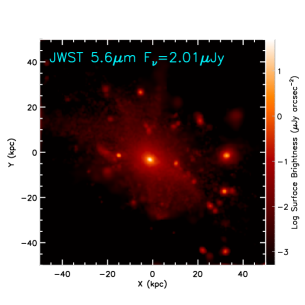
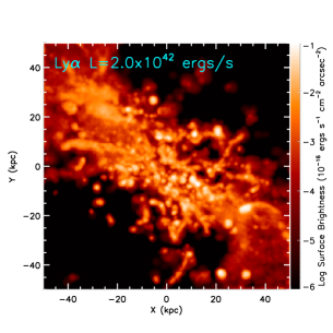
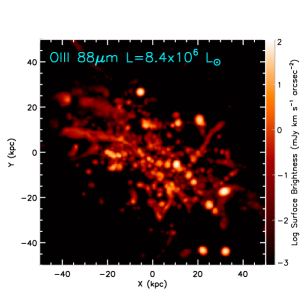
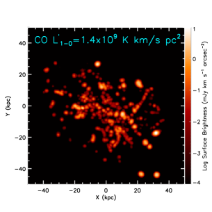
Figure 14: Surface brightness map of the most massive galaxy at redshift z=3.1 from the Milky Way Simulation post processed by ART², in JWST F560W filter, Ly$\alpha$, [CII], [NII], [OIII], and CO line, respectively. The legend in the image indicates the total flux from the entire field of view of the JWST filter, and total line luminosities for the Ly$\alpha$ [CII], [NII], [OIII] and the CO 1-0 transition, respectively.

.

The ART² code can be applied to most hydrodynamics simulations to obtain multi-wavelength properties of the simulated system. There are two approaches for the post processing: individual objects for detailed properties of discrete targets, and whole snapshot for statistical properties of the entire system. To demonstrate these two approaches, we apply ART² to two astrophysical simulations: the small-scale, zoom-in Milky Way Simulation (Zhu & Li, 2016), and the large-scale, full-box IllustrisTNG Simulation (Pillepich et al., 2018a; Springel et al., 2018; Marinacci et al., 2018; Naiman et al., 2018; Nelson et al., 2018, 2019a, 2019b; Pillepich et al., 2019).

For the first application, we obtain the output for each of the targeted galaxies, which contains the full spectral energy distribution (SED) in continuum from X-ray to far-infrared, fine structure lines from atoms and ions such as H, He, C, N, O, and other elements, resonant scattering Ly$\alpha$ line, and molecular lines such as CO, as well as images at different bands defined by filters of existing and future observatories such as HST and JWST. This data set is ideal to study of individual and statistical properties of galaxies at different redshift, luminosity functions, dust and gas properties, photon escape fractions, and relations between photometric properties and galaxy properties such as galaxy mass, star formation rate (SFR) and metallicity.

For the second application, we obtain the output for the entire system, which is ideal to study the global properties of the simulation box, such as ionization and intensity mappings. In this example, we focus on the intensity mappings of emission lines Ly$\alpha$, [CII], [NII], [OIII], and CO.

Since ART² is a Monte Carlo code, we use photons to trace the continuum RT and the resonant scattering of the Ly$\alpha$ photons, and we use rays to trace the non-LTE molecular and atomic line transfer. The number of continuum and Ly$\alpha$ photons varies between $10^{6}$ to $10^{8}$ depending on the number of grid cells generated from the hydrodynamics snapshots. For the non-LTE molecular and atomic fine structure lines, each finest cell in the adaptive grids initially has 48 rays, and the number of rays increases by a factor of 4 for each iteration until the level population reaches convergence. For a snapshot with $\sim 1\times 10^{6}$ cells, the typical total number of rays is $\sim 5\times 10^{7}$ for each of the line calculations.

In addition to the galaxy and gas properties from the hydrodynamics simulations, ART² requires the following additional inputs and assumptions. (1) The intrinsic stellar radiation is calculated with the stellar population synthesis code StarBurst99 (Leitherer et al., 1999, 2010, 2014) on a grid of stellar age and metallicity. (2) The black hole radiation is calculated using the accretion rate from the simulation assuming a double power law for spectral template of active galactic nuclei. (3) For the continuum RT, we assume a Milky Way dust opacity curve (Draine, 2003) and a dust-to-metal ratio of $10^{-2}$. (4) For CO line RT, a molecular fraction of $2\times 10^{-4}$ relative to H₂ is typically used, while the size of the molecular core of the cold clouds in our multi-phase ISM is calculated based on the local ionizing radiation flux.

The computational cost varies with application as different astrophysical system has different contents such as the number of objects and the distribution of gas density and radiation sources. Among the RT processes we consider, the CO molecular line calculation is typically the most time consuming module. Including 20 rotational levels in the statistical population equilibrium, and for a galaxy with $2\times 10^{6}$ cells, the molecular RT computation takes about 500 cpu-hours on the state-of-the-art CyberLAMP supercomputer cluster at Penn State.

For the Milky Way application, the largest galaxy at redshift z=3.1 has $5\times 10^{6}$ cells, the ART² calculations on this galaxy with all the modules (continuum, ionization, Lyman-alpha, atomic fine structure lines, and CO lines) required $\sim 20$ gigabytes RAM memory, and it took about 15 hours to run on 64 cores on the CyberLAMP cluster. For the IllustrisTNG application, the snapshot size is $\sim 1.7$ terabytes, so we selected a slice of 5 Mpc of the simulation box for the line intensity mapping, and it took ART² about 8 hours on 64 cores of the CyberLAMP cluster to calculate the lines.

We emphasize that these applications are intended to serve as proof-of-concept examples of the new ART² code in this work, an exploration of other assumptions and parameters such as supernovae dust models (e.g., Li et al., 2008; Marassi et al., 2019), and an in-depth analysis of the results or topics, will be presented in upcoming papers.

3.1 Application to the Zoom-in Milky Way Simulation

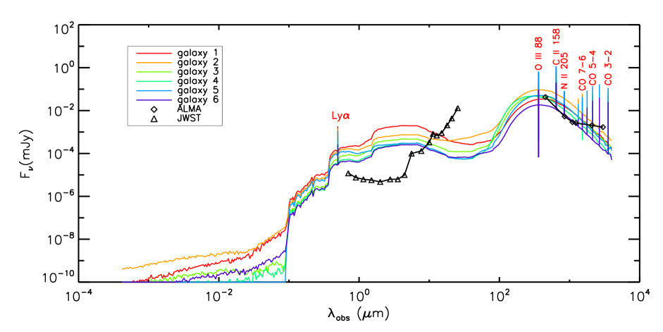
Figure 15: Full spectral energy distribution with continuum and lines for the 6 most massive galaxies at redshift z=3.1 from the Milky Way Simulation post processed by ART². The detection limits of JWST and ALMA are shown for comparison. Note galaxy #6 in the plot has strong [OIII] absorption line, while galaxy #4 has strong CO absorption lines.

The Milky Way Simulation was described in detail in Zhu & Li (2016), here we only give a brief summary of the simulation. It was a zoom-in hydrodynamics cosmological simulation run with the the Lagrangian Meshless Finite-Mass code Gizmo (Hopkins, 2015). A comprehensive list of physical processes was included in the simulation, including metal-dependent gas cooling, star formation, stellar evolution, chemical enrichment, and thermal and kinetic feedback from stars. This simulation did not include black holes.

The galaxy has a virial mass of $\sim 1.6\times 10^{12}\,\rm M_{\odot}$. The mass resolutions of the simulation are $\rm{m_{b}}=4\times 10^{5}\,\rm{M_{\odot}}$ for gas and star particles and $\rm{m_{dm}}=2.2\times 10^{6}\,\rm{M_{\odot}}$ for dark matter particles in the high resolution zoom-in region, and the gravitational softening length of gas particle is $\epsilon_{\rm{gas}}=0.5\,\rm{kpc}$. It was run with the following cosmological parameters: $\Omega_{\rm m}=0.25,\,\Omega_{\rm b}=0.04,\,\Omega_{\Lambda}=0.75,\,\sigma_{8}=0.9,\,n_{s}=1$ and a Hubble constant $\rm H=100\,h=73\,\rm{kms^{-1}Mpc^{-1}}$. The simulation was evolved from redshift $z=127$ to $z=0$, and in each snapshot, galaxies are identified as “groups" using the friend-of-friend group finder.

As an example to demonstrate the capability of ART², we randomly choose the snapshot at redshift z=3.1 We first extract out the 50 largest halos from the snapshot, construct the adaptive grid, and run all RT components on these galaxies. The ionization RT is run with the equilibrium ionization option,and all RT runs use the sub-grid multi-phase ISM model. Molecular line RT is done for CO only.

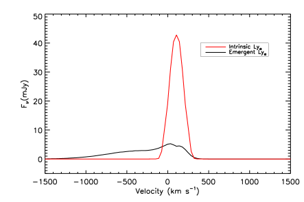
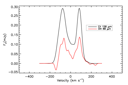
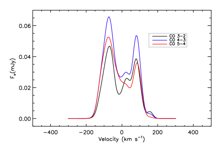
Figure 16: Line profiles of resonant scattering line Ly$\alpha$, atomic fine structure lines [CII] and [OIII], and molecular lines at transitions 5-4, 4-3, and 3-2, respectively, of the most massive galaxy at z=3.1 from the Milky Way Simulation.

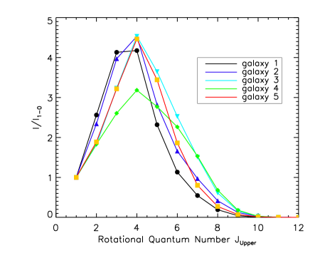
Figure 17: The excitation ladder of CO transitions for the 5 most massive galaxies at z=3.1 from the Milky Way Simulation.

3.1.1 Multi-wavelength SEDs and Images of Galaxies

The ART² calculation can produce multi-wavelength spectral energy distribution, which includes both continuum and emission (or absorption) lines, and images of galaxies and ISM, as demonstrated in the following figures. Figure 14 shows the images of the most massive galaxy as observed in the JWST 5.6 $\mu$m bands, Ly$\alpha$ resonant line, atomic fine structure lines [CII], [NII] and [OIII], and the molecular line CO $J=$1-0 transition, respectively. Figure 15 shows the overall SEDs, which include atomic and molecular lines and a continuum spanning 7 orders of magnitude in wavelength, of the 6 most massive galaxies at redshift z=3.1 of the Milky Way Simulation. The galaxies in this sample appear to be star-forming galaxies with strong lines of Ly$\alpha$, [OIII], [CII], [NII] and CO, with some having strong [OIII] or CO absorption lines due to high gas density in the galaxies.

3.1.2 Emission Line Properties of Galaxies

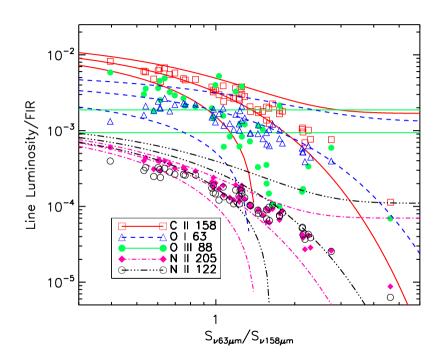
Figure 18: The line luminosity of [CII] 158 $\mu$m, [OI] 63 $\mu$m, [OIII] 88 $\mu$m, [NII] 122 $\mu$m, and [NII] 205 $\mu$m relative to the FIR luminosity between 8 and 1000 $\mu$m, as a function of the continuum flux ratio at 63 and 158 $\mu$m, $S_{\nu 63\mu m}$/$S_{\nu 158\mu m}$. The colored circles are the 50 most massive galaxies from the Milky Way Simulation, while the colored lines indicate the observed range of the relevant line from Díaz-Santos et al. (2017).

Figure 19: The [CII] emission from PDR relative to the total as a function of the continuum flux ratio at 63 and 158 $\mu$m for the 50 most massive galaxies from the Milky Way Simulation post processed by ART². The three straight lines represent the observed correlation and its scatter from Díaz-Santos et al. (2017).

The resonant scattering Ly$\alpha$ line, and the atomic fine structure lines such as [CII] and [OIII], and molecular lines such as CO are powerful lines to probe galaxies. Figure 16 shows the line profiles of Ly$\alpha$, [CII] and [OIII], and molecular CO lines at transitions 5-4, 4-3, and 3-2 of the most massive galaxy at z=3.1. Figure 17 showed the excitation ladder $\rm{I_{J-J-1}}/\rm{I_{1-0}}$ for the 5 most massive halos, which indicates the peak excitation is at $\rm J=4$.

The emission lines survey of nearby infrared luminous galaxies by (Díaz-Santos et al., 2017) shows an emission line deficit phenomenon in which the luminosity ratio between emission lines of [CII], [NII], [OII] and [OIII], and FIR emission decreases as dust temperature increases.

The fine structure atomic emission lines of [CII], [NII], [OII] and [OIII] are computed for the 50 most massive halos, and the line luminosities relative the FIR luminosity as a function of the continuum flux ratio at 63 and 158 $\mu$m, $S_{\nu 63\mu m}$/$S_{\nu 158\mu m}$, are plotted in Figure 18. The calculated luminosity ratios show the so called emission line deficit effect, and are generally consistent with the observations by Díaz-Santos et al. (2017).

In an attempt to understand the origin of the [CII] emission, Díaz-Santos et al. (2017) used the [NII] 220 $\mu$m emission as a proxy by to divide the [CII] 158 $\mu$m emission into two parts, one arising from the photodissociation region (PDR), and one arising from the ionized medium. The ionization emission is assumed to be 3 times that of the [NII] 220 $\mu$m luminosity using photoionization calculations as a guide. With such a prescription, the [CII] luminosity from PDR relative to the total is found to correlate with the dust temperature indicated by the flux ratio $S_{\nu 63\mu m}$/$S_{\nu 158\mu m}$.

In Figure 19 we compare this relation between our calculations and the observation. The slope of the calculated relation is somewhat smaller than the observed. However, given the larger scatter in the observed correlation, the calculation and the observation are still in broad agreement.

3.1.3 Statistical Properties and Correlations

Figure 20: Correlations between luminosities of FIR, Ly$\alpha$, [CII] and [OIII] and star formation rate of the 50 most massive galaxies at z=3.1 from the Milky Way Simulation.

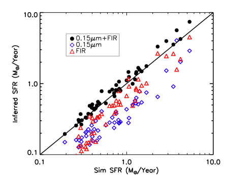
Figure 21: Calibration of SFR indicators based on the UV (green diamond) and FIR (red triangle) luminosities of the 50 most massive galaxies at z=3.1 from the Milky Way Simulation, and a linear combination of the two (black dot). The black line is the diagonal line for a perfect match of SFR from the two indicators.

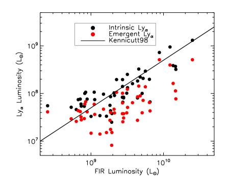
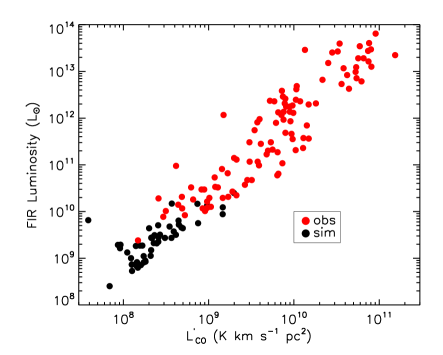
Figure 22: Correlation between Ly$\alpha$ and FIR luminosities (top), and between CO and FIR luminosities (bottom) of the 50 most massive galaxies at z=3.1 from the Milky Way Simulation, compared with the scaling relation of Kennicutt (1998) (top), and the observations of Solomon & Vanden Bout (2005) (bottom).

Figure 23: The relation between CO-to-H₂ mass conversion factor $\alpha$ and CO luminosity $\rm{L^{\prime}_{\rm CO}(1-0)}$ of the 50 most massive galaxies at z=3.1 from the Milky Way Simulation.

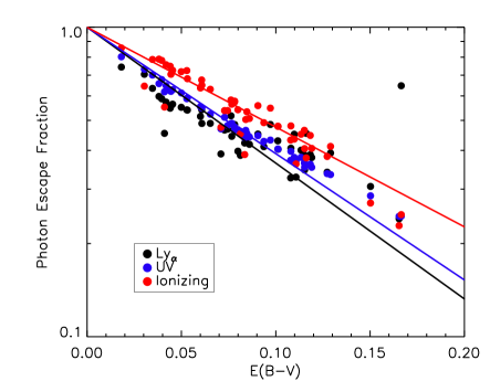
Figure 24: Correlation between escape fraction of the ionizing, UV (0.15 $\mu$m), and Ly$\alpha$ photons from the 50 most massive galaxies at z=3.1 from the Milky Way Simulation and the $B-V$ color excess $E(B-V)$. The lines are fittings for the respective photons.

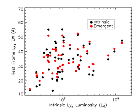
Figure 25: Intrinsic and emergent rest-frame equivalent widths of Ly$\alpha$ lines of the 50 most massive galaxies at z=3.1 from the Milky Way Simulation post processed by ART².

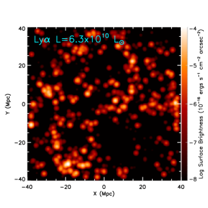
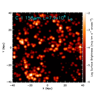
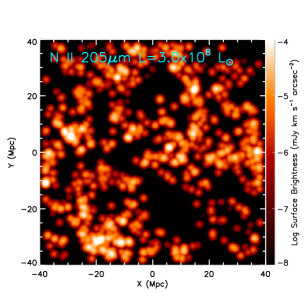
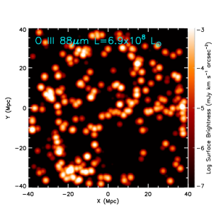
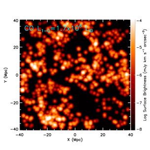
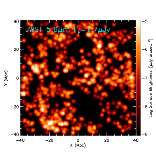
Figure 26: Intensity maps of resonant scattering line Ly$\alpha$, atomic fine structure lines [CII], [NII] and [OIII], molecular line CO (1-0), and continuum at JWST filter F560W, for a 5 Mpc slice at $z=8$ from the IllustrisTNG100 Simulation post-processed by ART².

The ART² data is ideal to study not only individual properties as shown in the previous sections, but also statistical properties of galaxies and ISM at different redshift, and when combined with data from the hydrodynamics simulation, we can study relations between photometric properties and galaxy properties such as galaxy mass, star formation rate and metallicity, as demonstrated in Figure 20, which shows the correlations between luminosities of FIR, Ly$\alpha$, [CII] and [OIII] and SFR of the 50 most massive galaxies in the simulation at redshift z=3.1.

Figure 21 shows the SFR indicator calibration using the UV (0.15 $\mu$mu) and FIR ($8-1000~{}\mu$m) luminosities. The inferred SFR from the FIR and UV, and a linear combination of the two are determined using the calibration given by Calzetti (2012). It is evident that the UV luminosity is a poor indicator of the SFR due to the dust extinction, while the FIR indicator works much better. However, the linear combination of the two has an even tighter correlation with the SFR obtained directly from the simulation.

Figure 22 shows the relation between Ly$\alpha$ and FIR (top), and between FIR and CO luminosity $\rm{L^{\prime}_{CO}(1-0)}$ (bottom). The intrinsic Ly$\alpha$ luminosity correlates with FIR tightly and agrees with the scaling relation proposed by Kennicutt (1998). However, the emergent Ly$\alpha$ luminosities are much lower due to the dust absorption. On the other hand, the correlation between CO and FIR luminosity from our simulations smoothly matches the observations of Solomon & Vanden Bout (2005), although the galaxies in the present simulations are typically smaller and have lower luminosities than from the observation sample.

The CO-to-H₂ mass conversion factor, $\alpha=\rm{M(H_{2})/L^{\prime}_{CO}}$, is an important parameter to understand star formation and the ISM in galaxies. However, measurements of the $\alpha$ factor show large scatterings in different galaxies (Bolatto et al., 2013). We show in Figure 23 the relation between the $\alpha$ factor and CO luminosity $\rm{L^{\prime}_{CO}(1-0)}$ of the 50 most massive galaxies at z=3.1 in the Milky Way Simulation post processed by ART². The average $\alpha$ factor from the simulation $\sim$ 2 M_⊙/K km s^-1 pc², which is consistent with the observed values of normal galaxies (Bolatto et al., 2013).

Figure 24 shows the escape fraction of the Ly$\alpha$, UV at 0.15 $\mu$m, and ionizing photons from the galaxies as a function of $E(B-V)$, for the 50 most galaxies in this sample.

Finally, Figure 25 shows the intrinsic and emergent rest-frame equivalent widths of Ly$\alpha$ lines from the simulation. The EW range of $10-60\,\AA$ is consistent with the EW range of star-forming galaxies at this redshift (Yajima et al., 2012c).

3.2 Application to the Large-scale IllustrisTNG Simulation

In this example, we apply ART² to the IllustrisTNG Simulation to demonstrate the technique of making large-scale line intensity mappings of interested lines such as Ly$\alpha$, [CII], [OIII], and CO. For each target redshift, we will divide the simulation snapshot into thin slices in the line of sight direction. The thickness of each slice corresponds to the frequency resolution element of the mapping experiment. The RT calculations are then performed for each slice, resulting the full spectrum including continuum and lines. The stacking of slices at different redshifts therefore results in a three-dimensional data cube similar to the observational data from intensity mapping experiments. Choices of different slices at the same redshift represent different realizations of the data cubes, and can be used to study the statistical variance. These simulated data cubes can be an important testbed for different analyses techniques, such as those for background and foreground contamination removal, and the models for the full-spectrum comic background radiation.

The IllustrisTNG Simulations are the state-of-the-art cosmological simulations currently available (Pillepich et al., 2018a; Springel et al., 2018; Marinacci et al., 2018; Naiman et al., 2018; Nelson et al., 2018, 2019a, 2019b; Pillepich et al., 2019). The simulations were carried out with the moving-mesh code Arepo (Springel, 2010; Springel et al., 2019). The list of physical processes is similar to that of the Milky Way Simulation (Zhu & Li, 2016) with additional physics of black hole accretion and feedback, and magnetic fields (Weinberger et al., 2017; Pillepich et al., 2018b).

We use the TNG100 Simulation in this work, which is publicly available (Nelson et al., 2019b). TNG100 has a box size of 100 Mpc, and the mass resolutions are $\rm{m_{b}}=1.4\times 10^{6}\,\rm{M_{\odot}}$ for baryons and $\rm{m_{dm}}=7.5\times 10^{6}\,\rm{M_{\odot}}$ for dark matter, and the minimum cell softening length is $\epsilon_{\rm gas}=0.18\,\rm{kpc}$. It was run with the Planck cosmological parameters Planck Collaboration et al. (2016): $\Omega_{\Lambda}=0.6911$, $\Omega_{\rm m}=0.3089$, $\Omega_{\rm b}=0.0486$, $\sigma_{8}=0.8159$, $n_{s}=0.9667$ and $h=0.6774$.

For the demonstration, we randomly choose the snapshot at redshift z=8, and a random slice of 5 Mpc in depth. We apply ART² to the slice to calculate the total luminosity of Ly$\alpha$, [CII], [OIII], and CO lines for the intensity maps, as well as the continuum at $5.6\,\mu\,m$ of JWST filter F560W for comparison. The resulting intensity maps are shown in Figure 26. These preliminary results show that Ly$\alpha$ is the strongest line to study the high-redshift galaxies, while the CO 1-0 line is weaker than the FIR lines [CII], [NII] and [OIII]. A more comprehensive study of line intensity mappings using the IllustrisTNG Simulations will be presented in a future paper.

4 Discussions and Conclusions

The new ART² implements a number of novel methods to calculate the non-LTE molecular and atomic line transfer and to parallelize the code. These treatments ensure accurate, efficient and self-consistent calculations of the continuum from sub-millimeter to X-ray, and various lines from atoms and molecules, such as Ly$\alpha$, [CII], [OIII], and CO. In addition, ART² adopts a multi-phase ISM model, which ensures an appropriate prescription of the ISM physics in case hydrodynamics simulations have insufficient resolution to resolve the multi-phase ISM, and it employs an adaptive grid scheme, which can handle arbitrary geometry and cover a large dynamical range of gas densities in hydrodynamical simulations. These essential features make ART² a multi-purpose code to study the multi-wavelength properties of a wide range of astrophysical systems, from planetary disks, to star forming regions, to galaxies, and to large-scale structures of the Universe.

To demonstrate the capability of the new ART², we applied it to two hydrodynamics cosmological simulations, the zoom-in Milky Way Simulation to obtain the multi-band properties of individual galaxies at different redshift, and the full-box IllustrisTNG100 Simulation to obtain line intensity maps of Ly$\alpha$, [CII], [NII], [OIII] and CO lines and continuum JWST F560W. The RT outputs include multi-wavelength SEDs, lines and images, useful for an array of studies such as the correlations between physical and photometric properties, the physical conditions of line emission, the origin of emission line deficit observed in galaxies, the escape fraction of ionizing and UV photons, the luminosity functions, and the evolution of the multi-band properties of galaxies and gas with time.

We will perform in-depth studies of the above topics with the comprehensive IllustrisTNG $+$ ART² (ILART) Project, in which we will post process the IllustrisTNG100 Simulation with ART² to derive multi-band properties of galaxies and ISM at different redshifts. In addition, we will also apply ART² to IllustrisTNG50, which has the highest resolutions of all TNG runs ($\rm{m_{b}}=8.5\times 10^{4}\,\rm{M}_{\odot},\rm{m_{dm}}=4.6\times 10^{5}\,\rm{M}_{\odot},\epsilon_{\rm{gas}}=0.18\,\rm{kpc}$), and which is expected to be released to the public sometime in the near future (private communication with Dr. Dylan Nelson). The ILART Project is expected to provide new insights into a wide array of studies, as well as effects of numerical resolutions on the RT results, in upcoming papers.

To conclude, ART² is well-suited to study both individual objects and global properties of the entire system. It enables direct comparison between numerical simulations and multi-band observations, and it will provide a crucial theoretical framework for the understanding of existing multi-band astronomical observations, the design and plan for future surveys, and the synergy between multi-band galaxy surveys and line intensity mappings to provide a full picture of the origin and evolution of the Universe. Therefore, ART² can provide a powerful and versatile tool to bridge the gap between theories and observations of the cosmic structures.

References

- Aird et al. (2019) Aird, J., Coil, A. L., & Georgakakis, A. 2019, MNRAS, 484, 4360
- Allen et al. (2008) Allen, M. G., Groves, B. A., Dopita, M. A., Sutherland, R. S., & Kewley, L. J. 2008, ApJS, 178, 20
- Arata et al. (2020) Arata, S., Yajima, H., Nagamine, K., Abe, M., & Khochfar, S. 2020, arXiv e-prints, arXiv:2001.01853
- Arata et al. (2019) Arata, S., Yajima, H., Nagamine, K., Li, Y., & Khochfar, S. 2019, MNRAS, 488, 2629
- Bernal et al. (2019) Bernal, J. L., Breysse, P. C., & Kovetz, E. D. 2019, Phys. Rev. Lett., 123, 251301
- Bjorkman & Wood (2001) Bjorkman, J. E., & Wood, K. 2001, ApJ, 554, 615
- Bolatto et al. (2013) Bolatto, A. D., Wolfire, M., & Leroy, A. K. 2013, ARA&A, 51, 207
- Bouwens et al. (2014) Bouwens, R. J., Illingworth, G. D., Oesch, P. A., Labbé, I., van Dokkum, P. G., Trenti, M., Franx, M., Smit, R., Gonzalez, V., & Magee, D. 2014, ApJ, 793, 115
- Brinch & Hogerheijde (2010) Brinch, C., & Hogerheijde, M. R. 2010, A&A, 523, A25
- Calzetti (2012) Calzetti, D. 2012, ArXiv e-prints
- Camps & Baes (2015) Camps, P., & Baes, M. 2015, Astronomy and Computing, 9, 20
- Chung et al. (2019) Chung, D. T., Viero, M. P., Church, S. E., Wechsler, R. H., Alvarez, M. A., Bond, J. R., Breysse, P. C., Cleary, K. A., Eriksen, H. K., Foss, M. K., Gundersen, J. O., Harper, S. E., Ihle, H. T., Keating, L. C., Murray, N., Padmanabhan, H., Stein, G. F., Wehus, I. K., & COMAP Collaboration. 2019, ApJ, 872, 186
- Cooray et al. (2019) Cooray, A., Aguirre, J., Ali-Haimoud, Y., Alvarez, M., Appleton, P., Armus, L., Becker, G., Bock, J., Bowler, R., Bowman, J., Bradford, M., Breysse, P., Bromm, V., Burns, J., Caputi, K., Castellano, M., Chang, T.-C., Chary, R., Chiang, H., Cohn, J., Conselice, C., Cuby, J.-G., Davies, F., Dayal, P., Dore, O., Farrah, D., Ferrara, A., Finkelstein, S., Furlanetto, S., Hazelton, B., Heneka, C., Hutter, A., Jacobs, D., Koopmans, L., Kovetz, E., La Piante, P., Le Fevre, O., Liu, A., Ma, J., Ma, Y.-Z., Malhotra, S., Mao, Y., Marrone, D., Masui, K., McQuinn, M., Mirocha, J., Mortlock, D., Murphy, E., Nayyeri, H., Natarajan, P., Nithyanand an, T., Parsons, A., Pello, R., Pope, A., Rhoads, J., Rhodes, J., Riechers, D., Robertson, B., Scarlata, C., Serjeant, S., Saliwanchik, B., Salvaterra, R., Schneider, R., Silva, M., Sahlén, M., Santos, M. G., Switzer, E., Temi, P., Trac, H., Venkatesan, A., Visbal, E., Zaldarriaga, M., Zemcov, M., & Zheng, Z. 2019, BAAS, 51, 48
- Crain et al. (2015) Crain, R. A., Schaye, J., Bower, R. G., Furlong, M., Schaller, M., Theuns, T., Dalla Vecchia, C., Frenk, C. S., McCarthy, I. G., Helly, J. C., Jenkins, A., Rosas-Guevara, Y. M., White, S. D. M., & Trayford, J. W. 2015, MNRAS, 450, 1937
- Davé et al. (2019) Davé, R., Anglés-Alcázar, D., Narayanan, D., Li, Q., Rafieferantsoa, M. H., & Appleby, S. 2019, MNRAS, 486, 2827
- de Jong et al. (1975) de Jong, T., Dalgarno, A., & Chu, S.-I. 1975, ApJ, 199, 69
- Decarli et al. (2018) Decarli, R., Walter, F., Venemans, B. P., Bañados, E., Bertoldi, F., Carilli, C., Fan, X., Farina, E. P., Mazzucchelli, C., Riechers, D., Rix, H.-W., Strauss, M. A., Wang, R., & Yang, Y. 2018, ApJ, 854, 97
- Díaz-Santos et al. (2017) Díaz-Santos, T., Armus, L., Charmandaris, V., Lu, N., Stierwalt, S., Stacey, G., Malhotra, S., van der Werf, P. P., Howell, J. H., Privon, G. C., Mazzarella, J. M., Goldsmith, P. F., Murphy, E. J., Barcos-Muñoz, L., Linden, S. T., Inami, H., Larson, K. L., Evans, A. S., Appleton, P., Iwasawa, K., Lord, S., Sanders, D. B., & Surace, J. A. 2017, ApJ, 846, 32
- Dijkstra et al. (2016) Dijkstra, M., Gronke, M., & Sobral, D. 2016, ApJ, 823, 74
- Dolag et al. (2016) Dolag, K., Komatsu, E., & Sunyaev, R. 2016, MNRAS, 463, 1797
- Draine (2003) Draine, B. T. 2003, ARA&A, 41, 241
- Dubois et al. (2014) Dubois, Y., Pichon, C., Welker, C., Le Borgne, D., Devriendt, J., Laigle, C., Codis, S., Pogosyan, D., Arnouts, S., Benabed, K., Bertin, E., Blaizot, J., Bouchet, F., Cardoso, J. F., Colombi, S., de Lapparent, V., Desjacques, V., Gavazzi, R., Kassin, S., Kimm, T., McCracken, H., Milliard, B., Peirani, S., Prunet, S., Rouberol, S., Silk, J., Slyz, A., Sousbie, T., Teyssier, R., Tresse, L., Treyer, M., Vibert, D., & Volonteri, M. 2014, MNRAS, 444, 1453
- Dullemond et al. (2012) Dullemond, C. P., Juhasz, A., Pohl, A., Sereshti, F., Shetty, R., Peters, T., Commercon, B., & Flock, M. 2012, RADMC-3D: A multi-purpose radiative transfer tool
- Feng et al. (2016) Feng, Y., Di-Matteo, T., Croft, R. A., Bird, S., Battaglia, N., & Wilkins, S. 2016, MNRAS, 455, 2778
- Ferland et al. (2017) Ferland, G. J., Chatzikos, M., Guzmán, F., Lykins, M. L., van Hoof, P. A. M., Williams, R. J. R., Abel, N. P., Badnell, N. R., Keenan, F. P., Porter, R. L., & Stancil, P. C. 2017, Rev. Mex. Astron. Astrofis., 53, 385
- Fonseca et al. (2017) Fonseca, J., Silva, M. B., Santos, M. G., & Cooray, A. 2017, MNRAS, 464, 1948
- Genel et al. (2014) Genel, S., Vogelsberger, M., Springel, V., Sijacki, D., Nelson, D., Snyder, G., Rodriguez-Gomez, V., Torrey, P., & Hernquist, L. 2014, MNRAS, 445, 175
- Goldreich & Kwan (1974) Goldreich, P., & Kwan, J. 1974, ApJ, 189, 441
- Goto et al. (2019) Goto, T., Oi, N., Utsumi, Y., Momose, R., Matsuhara, H., Hashimoto, T., Toba, Y., Ohyama, Y., Takagi, T., Chiang, C.-Y., Kim, S. J., Kilerci Eser, E., Malkan, M., Kim, H., Miyaji, T., Im, M., Nakagawa, T., Jeong, W.-S., Pearson, C., Barrufet, L., Sedgwick, C., Burgarella, D., Buat, V., & Ikeda, H. 2019, PASJ, 71, 30
- Grand et al. (2017) Grand, R. J. J., Gómez, F. A., Marinacci, F., Pakmor, R., Springel, V., Campbell, D. J. R., Frenk, C. S., Jenkins, A., & White, S. D. M. 2017, MNRAS, 467, 179
- Gray et al. (2015) Gray, W. J., Scannapieco, E., & Kasen, D. 2015, ApJ, 801, 107
- Hansen & Oh (2006) Hansen, M., & Oh, S. P. 2006, MNRAS, 367, 979
- Hariharan et al. (2017) Hariharan, N., Graziani, L., Ciardi, B., Miniati, F., & Bungartz, H. J. 2017, MNRAS, 467, 2458
- Hickox & Alexander (2018) Hickox, R. C., & Alexander, D. M. 2018, ARA&A, 56, 625
- Hill et al. (2018) Hill, R., Masui, K. W., & Scott, D. 2018, Applied Spectroscopy, 72, 663
- Hobson & Padman (1993) Hobson, M. P., & Padman, R. 1993, MNRAS, 264, 161
- Hogerheijde & van der Tak (2000a) Hogerheijde, M., & van der Tak, F. 2000a, RATRAN: Radiative Transfer and Molecular Excitation in One and Two Dimensions
- Hogerheijde & van der Tak (2000b) Hogerheijde, M. R., & van der Tak, F. F. S. 2000b, A&A, 362, 697
- Hopkins (2015) Hopkins, P. F. 2015, MNRAS, 450, 53
- Hopkins et al. (2018) Hopkins, P. F., Wetzel, A., Kereš, D., Faucher-Giguère, C.-A., Quataert, E., Boylan-Kolchin, M., Murray, N., Hayward, C. C., Garrison-Kimmel, S., Hummels, C., Feldmann, R., Torrey, P., Ma, X., Anglés-Alcázar, D., Su, K.-Y., Orr, M., Schmitz, D., Escala, I., Sanderson, R., Grudić, M. Y., Hafen, Z., Kim, J.-H., Fitts, A., Bullock, J. S., Wheeler, C., Chan, T. K., Elbert, O. D., & Narayanan, D. 2018, MNRAS, 480, 800
- Karkare & Bird (2018) Karkare, K. S., & Bird, S. 2018, Phys. Rev. D, 98, 043529
- Kennicutt (1998) Kennicutt, Jr., R. C. 1998, ApJ, 498, 541
- Keto & Rybicki (2010) Keto, E., & Rybicki, G. 2010, ApJ, 716, 1315
- Kewley et al. (2019) Kewley, L. J., Nicholls, D. C., & Sutherland, R. S. 2019, ARA&A, 57, 511
- Koprowski et al. (2017) Koprowski, M. P., Dunlop, J. S., Michałowski, M. J., Coppin, K. E. K., Geach, J. E., McLure, R. J., Scott, D., & van der Werf, P. P. 2017, MNRAS, 471, 4155
- Kovetz et al. (2019) Kovetz, E., Breysse, P. C., Lidz, A., Bock, J., Bradford, C. M., Chang, T.-C., Foreman, S., Padmanabhan, H., Pullen, A., Riechers, D., Silva, M. B., & Switzer, E. 2019, BAAS, 51, 101
- Kovetz et al. (2017) Kovetz, E. D., Viero, M. P., Lidz, A., Newburgh, L., Rahman, M., Switzer, E., Kamionkowski, M., Aguirre, J., Alvarez, M., Bock, J., Bond, J. R., Bower, G., Bradford, C. M., Breysse, P. C., Bull, P., Chang, T.-C., Cheng, Y.-T., Chung, D., Cleary, K., Corray, A., Crites, A., Croft, R., Doré, O., Eastwood, M., Ferrara, A., Fonseca, J., Jacobs, D., Keating, G. K., Lagache, G., Lakhlani, G., Liu, A., Moodley, K., Murray, N., Pénin, A., Popping, G., Pullen, A., Reichers, D., Saito, S., Saliwanchik, B., Santos, M., Somerville, R., Stacey, G., Stein, G., Villaescusa-Navarro, F., Visbal, E., Weltman, A. a., Wolz, L., & Zemcov, M. 2017, arXiv e-prints, arXiv:1709.09066
- Krumholz (2014) Krumholz, M. R. 2014, MNRAS, 437, 1662
- Laursen (2011) Laursen, P. 2011, IGMtransfer: Intergalactic Radiative Transfer Code
- Leitherer et al. (2014) Leitherer, C., Ekström, S., Meynet, G., Schaerer, D., Agienko, K. B., & Levesque, E. M. 2014, ApJS, 212, 14
- Leitherer et al. (2010) Leitherer, C., Ortiz Otálvaro, P. A., Bresolin, F., Kudritzki, R.-P., Lo Faro, B., Pauldrach, A. W. A., Pettini, M., & Rix, S. A. 2010, ApJS, 189, 309
- Leitherer et al. (1999) Leitherer, C., Schaerer, D., Goldader, J. D., Delgado, R. M. G., Robert, C., Kune, D. F., de Mello, D. F., Devost, D., & Heckman, T. M. 1999, ApJS, 123, 3
- Li et al. (2008) Li, Y., Hopkins, P. F., Hernquist, L., Finkbeiner, D. P., Cox, T. J., Springel, V., Jiang, L., Fan, X., & Yoshida, N. 2008, ApJ, 678, 41
- Lidz et al. (2011) Lidz, A., Furlanetto, S. R., Oh, S. P., Aguirre, J., Chang, T.-C., Doré, O., & Pritchard, J. R. 2011, ApJ, 741, 70
- Madau & Dickinson (2014) Madau, P., & Dickinson, M. 2014, ARA&A, 52, 415
- Marassi et al. (2019) Marassi, S., Schneider, R., Limongi, M., Chieffi, A., Graziani, L., & Bianchi, S. 2019, MNRAS, 484, 2587
- Marinacci et al. (2018) Marinacci, F., Vogelsberger, M., Pakmor, R., Torrey, P., Springel, V., Hernquist, L., Nelson, D., Weinberger, R., Pillepich, A., Naiman, J., & Genel, S. 2018, MNRAS, 480, 5113
- Megeath et al. (2019) Megeath, S. T., Armus, L., Bentz, M., Binder, B., Civano, F., Corrales, L., Dragomir, D., Elvis, M., Espaillat, C., Finkelstein, S., Fox, D., Greenhouse, M., Hoadley, K., Kauffmann, J., Kirkpatrick, A., Kraft, R., Khullar, G., Hartigan, P., Lillie, C., Lazio, J., Marengo, M., McCand liss, S., Meyer, M., Mushotzky, R., Pope, A., Roming, P., Smith, J. D., Stevenson, K., Tielens, A., Tremblay, G., Wang, D., & Wolk, S. 2019, in BAAS, Vol. 51, 184
- Moradinezhad Dizgah & Keating (2019) Moradinezhad Dizgah, A., & Keating, G. K. 2019, ApJ, 872, 126
- Naiman et al. (2018) Naiman, J. P., Pillepich, A., Springel, V., Ramirez-Ruiz, E., Torrey, P., Vogelsberger, M., Pakmor, R., Nelson, D., Marinacci, F., Hernquist, L., Weinberger, R., & Genel, S. 2018, MNRAS, 477, 1206
- Narayanan et al. (2009) Narayanan, D., Cox, T. J., Hayward, C. C., Younger, J. D., & Hernquist, L. 2009, MNRAS, 400, 1919
- Narayanan et al. (2011) Narayanan, D., Krumholz, M., Ostriker, E. C., & Hernquist, L. 2011, MNRAS, 418, 664
- Nelson et al. (2019a) Nelson, D., Pillepich, A., Springel, V., Pakmor, R., Weinberger, R., Genel, S., Torrey, P., Vogelsberger, M., Marinacci, F., & Hernquist, L. 2019a, MNRAS, 490, 3234
- Nelson et al. (2018) Nelson, D., Pillepich, A., Springel, V., Weinberger, R., Hernquist, L., Pakmor, R., Genel, S., Torrey, P., Vogelsberger, M., Kauffmann, G., Marinacci, F., & Naiman, J. 2018, MNRAS, 475, 624
- Nelson et al. (2019b) Nelson, D., Springel, V., Pillepich, A., Rodriguez-Gomez, V., Torrey, P., Genel, S., Vogelsberger, M., Pakmor, R., Marinacci, F., Weinberger, R., Kelley, L., Lovell, M., Diemer, B., & Hernquist, L. 2019b, Computational Astrophysics and Cosmology, 6, 2
- Neufeld (1990) Neufeld, D. A. 1990, ApJ, 350, 216
- Neufeld (1991) —. 1991, ApJ, 370, L85
- Park et al. (2019) Park, J., Mesinger, A., Greig, B., & Gillet, N. 2019, MNRAS, 484, 933
- Pillepich et al. (2018a) Pillepich, A., Nelson, D., Hernquist, L., Springel, V., Pakmor, R., Torrey, P., Weinberger, R., Genel, S., Naiman, J. P., Marinacci, F., & Vogelsberger, M. 2018a, MNRAS, 475, 648
- Pillepich et al. (2019) Pillepich, A., Nelson, D., Springel, V., Pakmor, R., Torrey, P., Weinberger, R., Vogelsberger, M., Marinacci, F., Genel, S., van der Wel, A., & Hernquist, L. 2019, MNRAS, 490, 3196
- Pillepich et al. (2018b) Pillepich, A., Springel, V., Nelson, D., Genel, S., Naiman, J., Pakmor, R., Hernquist, L., Torrey, P., Vogelsberger, M., Weinberger, R., & Marinacci, F. 2018b, MNRAS, 473, 4077
- Planck Collaboration et al. (2016) Planck Collaboration, Ade, P. A. R., Aghanim, N., Arnaud, M., Ashdown, M., Aumont, J., Baccigalupi, C., Banday, A. J., Barreiro, R. B., Bartlett, J. G., Bartolo, N., Battaner, E., Battye, R., Benabed, K., Benoît, A., Benoit-Lévy, A., Bernard, J. P., Bersanelli, M., Bielewicz, P., Bock, J. J., Bonaldi, A., Bonavera, L., Bond, J. R., Borrill, J., Bouchet, F. R., Boulanger, F., Bucher, M., Burigana, C., Butler, R. C., Calabrese, E., Cardoso, J. F., Catalano, A., Challinor, A., Chamballu, A., Chary, R. R., Chiang, H. C., Chluba, J., Christensen, P. R., Church, S., Clements, D. L., Colombi, S., Colombo, L. P. L., Combet, C., Coulais, A., Crill, B. P., Curto, A., Cuttaia, F., Danese, L., Davies, R. D., Davis, R. J., de Bernardis, P., de Rosa, A., de Zotti, G., Delabrouille, J., Désert, F. X., Di Valentino, E., Dickinson, C., Diego, J. M., Dolag, K., Dole, H., Donzelli, S., Doré, O., Douspis, M., Ducout, A., Dunkley, J., Dupac, X., Efstathiou, G., Elsner, F., Enßlin, T. A., Eriksen, H. K., Farhang, M., Fergusson, J., Finelli, F., Forni, O., Frailis, M., Fraisse, A. A., Franceschi, E., Frejsel, A., Galeotta, S., Galli, S., Ganga, K., Gauthier, C., Gerbino, M., Ghosh, T., Giard, M., Giraud-Héraud, Y., Giusarma, E., Gjerløw, E., González-Nuevo, J., Górski, K. M., Gratton, S., Gregorio, A., Gruppuso, A., Gudmundsson, J. E., Hamann, J., Hansen, F. K., Hanson, D., Harrison, D. L., Helou, G., Henrot-Versillé, S., Hernández-Monteagudo, C., Herranz, D., Hildebrand t, S. R., Hivon, E., Hobson, M., Holmes, W. A., Hornstrup, A., Hovest, W., Huang, Z., Huffenberger, K. M., Hurier, G., Jaffe, A. H., Jaffe, T. R., Jones, W. C., Juvela, M., Keihänen, E., Keskitalo, R., Kisner, T. S., Kneissl, R., Knoche, J., Knox, L., Kunz, M., Kurki-Suonio, H., Lagache, G., Lähteenmäki, A., Lamarre, J. M., Lasenby, A., Lattanzi, M., Lawrence, C. R., Leahy, J. P., Leonardi, R., Lesgourgues, J., Levrier, F., Lewis, A., Liguori, M., Lilje, P. B., Linden-Vørnle, M., López-Caniego, M., Lubin, P. M., Macías-Pérez, J. F., Maggio, G., Maino, D., Mandolesi, N., Mangilli, A., Marchini, A., Maris, M., Martin, P. G., Martinelli, M., Martínez-González, E., Masi, S., Matarrese, S., McGehee, P., Meinhold, P. R., Melchiorri, A., Melin, J. B., Mendes, L., Mennella, A., Migliaccio, M., Millea, M., Mitra, S., Miville-Deschênes, M. A., Moneti, A., Montier, L., Morgante, G., Mortlock, D., Moss, A., Munshi, D., Murphy, J. A., Naselsky, P., Nati, F., Natoli, P., Netterfield, C. B., Nørgaard-Nielsen, H. U., Noviello, F., Novikov, D., Novikov, I., Oxborrow, C. A., Paci, F., Pagano, L., Pajot, F., Paladini, R., Paoletti, D., Partridge, B., Pasian, F., Patanchon, G., Pearson, T. J., Perdereau, O., Perotto, L., Perrotta, F., Pettorino, V., Piacentini, F., Piat, M., Pierpaoli, E., Pietrobon, D., Plaszczynski, S., Pointecouteau, E., Polenta, G., Popa, L., Pratt, G. W., Prézeau, G., Prunet, S., Puget, J. L., Rachen, J. P., Reach, W. T., Rebolo, R., Reinecke, M., Remazeilles, M., Renault, C., Renzi, A., Ristorcelli, I., Rocha, G., Rosset, C., Rossetti, M., Roudier, G., Rouillé d’Orfeuil, B., Rowan-Robinson, M., Rubiño-Martín, J. A., Rusholme, B., Said, N., Salvatelli, V., Salvati, L., Sandri, M., Santos, D., Savelainen, M., Savini, G., Scott, D., Seiffert, M. D., Serra, P., Shellard, E. P. S., Spencer, L. D., Spinelli, M., Stolyarov, V., Stompor, R., Sudiwala, R., Sunyaev, R., Sutton, D., Suur-Uski, A. S., Sygnet, J. F., Tauber, J. A., Terenzi, L., Toffolatti, L., Tomasi, M., Tristram, M., Trombetti, T., Tucci, M., Tuovinen, J., Türler, M., Umana, G., Valenziano, L., Valiviita, J., Van Tent, F., Vielva, P., Villa, F., Wade, L. A., Wandelt, B. D., Wehus, I. K., White, M., White, S. D. M., Wilkinson, A., Yvon, D., Zacchei, A., & Zonca, A. 2016, A&A, 594, A13
- Pullen et al. (2014) Pullen, A. R., Doré, O., & Bock, J. 2014, ApJ, 786, 111
- Riechers et al. (2019) Riechers, D. A., Pavesi, R., Sharon, C. E., Hodge, J. A., Decarli, R., Walter, F., Carilli, C. L., Aravena, M., da Cunha, E., Daddi, E., Dickinson, M., Smail, I., Capak, P. L., Ivison, R. J., Sargent, M., Scoville, N. Z., & Wagg, J. 2019, ApJ, 872, 7
- Rosdahl et al. (2018) Rosdahl, J., Katz, H., Blaizot, J., Kimm, T., Michel-Dansac, L., Garel, T., Haehnelt, M., Ocvirk, P., & Teyssier, R. 2018, MNRAS, 479, 994
- Rundle et al. (2010) Rundle, D., Harries, T. J., Acreman, D. M., & Bate, M. R. 2010, MNRAS, 407, 986
- Rybicki & Lightman (1986) Rybicki, G. B., & Lightman, A. P. 1986, Radiative Processes in Astrophysics
- Schaerer et al. (2011) Schaerer, D., Hayes, M., Verhamme, A., & Teyssier, R. 2011, A&A, 531, A12
- Schaye et al. (2015) Schaye, J., Crain, R. A., Bower, R. G., Furlong, M., Schaller, M., Theuns, T., Dalla Vecchia, C., Frenk, C. S., McCarthy, I. G., Helly, J. C., Jenkins, A., Rosas-Guevara, Y. M., White, S. D. M., Baes, M., Booth, C. M., Camps, P., Navarro, J. F., Qu, Y., Rahmati, A., Sawala, T., Thomas, P. A., & Trayford, J. 2015, MNRAS, 446, 521
- Scoville et al. (2017) Scoville, N., Lee, N., Vanden Bout, P., Diaz-Santos, T., Sanders, D., Darvish, B., Bongiorno, A., Casey, C. M., Murchikova, L., Koda, J., Capak, P., Vlahakis, C., Ilbert, O., Sheth, K., Morokuma-Matsui, K., Ivison, R. J., Aussel, H., Laigle, C., McCracken, H. J., Armus, L., Pope, A., Toft, S., & Masters, D. 2017, ApJ, 837, 150
- Solomon et al. (1987) Solomon, P. M., Rivolo, A. R., Barrett, J., & Yahil, A. 1987, ApJ, 319, 730
- Solomon & Vanden Bout (2005) Solomon, P. M., & Vanden Bout, P. A. 2005, ARA&A, 43, 677
- Spitzer (1978) Spitzer, L. 1978, Physical processes in the interstellar medium
- Springel (2005) Springel, V. 2005, MNRAS, 364, 1105
- Springel (2010) —. 2010, MNRAS, 401, 791
- Springel & Hernquist (2003) Springel, V., & Hernquist, L. 2003, MNRAS, 339, 289
- Springel et al. (2018) Springel, V., Pakmor, R., Pillepich, A., Weinberger, R., Nelson, D., Hernquist, L., Vogelsberger, M., Genel, S., Torrey, P., Marinacci, F., & Naiman, J. 2018, MNRAS, 475, 676
- Springel et al. (2019) Springel, V., Pakmor, R., & Weinberger, R. 2019, AREPO: Cosmological magnetohydrodynamical moving-mesh simulation code
- Steinacker et al. (2013) Steinacker, J., Baes, M., & Gordon, K. D. 2013, ARA&A, 51, 63
- Sun et al. (2019) Sun, G., Hensley, B. S., Chang, T.-C., Doré, O., & Serra, P. 2019, ApJ, 887, 142
- Tremmel et al. (2017) Tremmel, M., Karcher, M., Governato, F., Volonteri, M., Quinn, T. R., Pontzen, A., Anderson, L., & Bellovary, J. 2017, MNRAS, 470, 1121
- van Zadelhoff et al. (2002) van Zadelhoff, G.-J., Dullemond, C. P., van der Tak, F. F. S., Yates, J. A., Doty, S. D., Ossenkopf, V., Hogerheijde, M. R., Juvela, M., Wiesemeyer, H., & Schöier, F. L. 2002, A&A, 395, 373
- Visbal et al. (2011) Visbal, E., Trac, H., & Loeb, A. 2011, J. Cosmology Astropart. Phys., 2011, 010
- Vogelsberger et al. (2014) Vogelsberger, M., Genel, S., Springel, V., Torrey, P., Sijacki, D., Xu, D., Snyder, G., Bird, S., Nelson, D., & Hernquist, L. 2014, Nature, 509, 177
- Weinberger et al. (2017) Weinberger, R., Springel, V., Hernquist, L., Pillepich, A., Marinacci, F., Pakmor, R., Nelson, D., Genel, S., Vogelsberger, M., Naiman, J., & Torrey, P. 2017, MNRAS, 465, 3291
- Wilkins et al. (2019) Wilkins, S. M., Lovell, C. C., & Stanway, E. R. 2019, MNRAS, 2490
- Yajima & Li (2014) Yajima, H., & Li, Y. 2014, MNRAS, 445, 3674
- Yajima et al. (2013) Yajima, H., Li, Y., & Zhu, Q. 2013, ApJ, 773, 151
- Yajima et al. (2012a) Yajima, H., Li, Y., Zhu, Q., & Abel, T. 2012a, MNRAS, 424, 884
- Yajima et al. (2012b) —. 2012b, MNRAS, 424, 884
- Yajima et al. (2015) —. 2015, ApJ, 801, 52
- Yajima et al. (2012c) Yajima, H., Li, Y., Zhu, Q., Abel, T., Gronwall, C., & Ciardullo, R. 2012c, ApJ, 754, 118
- Yajima et al. (2018) Yajima, H., Sugimura, K., & Hasegawa, K. 2018, MNRAS, 477, 5406
- Zheng et al. (2010) Zheng, Z., Cen, R., Trac, H., & Miralda-Escudé, J. 2010, ApJ, 716, 574
- Zheng et al. (2011) —. 2011, ApJ, 726, 38
- Zhu & Li (2016) Zhu, Q., & Li, Y. 2016, ApJ, 831, 52