A Graph-Based Approach for Active Learning in Regression

Abstract

Active learning aims to reduce labeling efforts by selectively asking humans to annotate the most important data points from an unlabeled pool and is an example of human-machine interaction. Though active learning has been extensively researched for classification and ranking problems, it is relatively understudied for regression problems. Most existing active learning for regression methods use the regression function learned at each active learning iteration to select the next informative point to query. This introduces several challenges such as handling noisy labels, parameter uncertainty and overcoming initially biased training data. Instead, we propose a feature-focused approach that formulates both sequential and batch-mode active regression as a novel bipartite graph optimization problem. We conduct experiments on both noise-free and noisy settings. Our experimental results on benchmark data sets demonstrate the effectiveness of our proposed approach.

Keywords: Active learning, bipartite graphs, regression, approximation algorithm, noisy data

1 Introduction

Supervised learning methods assume a large well-annotated training set. However, in many real-world applications, labeled data is often difficult and expensive to obtain, but we may have a large pool of unlabeled data. In such settings, active learning can be used where the machine learns an initial model from the labeled data, and then repetitively asks a human to annotate instances from the unlabeled pool.

Active learning has been extensively studied for classification and is most useful in settings where there are limited training annotations [1, 2, 3, 4, 5, 7]. However, there are several limitations with existing active learning: 1) Most works focus on classifications with relatively few works for regression. 2) Most works in active regression are model-focused; they use the learned regression function to select the next query point. Regression is an under-studied problem by the research community but extensively used in practice due to its ease of use and interpretability.

The limitations of being model focused are subtle but important. For example, as the query depends on the model if the previous point queried is incorrectly labeled by the domain expert, then it can produce undesirable results including even increasing model error. Most active learning for regression studies [8, 9, 10, 11, 12] assume that the annotations are accurate and focus on selecting the most informative point to query based on the newly learned function at each iteration. However, the labelers in the real world usually make noisy annotations, especially for regression tasks [13, 14]. Furthermore, the model-based methods could be highly biased when initial labeled data is limited as we discuss in Section 6. We use the term challenging regression settings to denote the regression problems where initial labeled data is limited and noisy due to human annotations.

In this paper, we propose a feature-focused active sampling strategy that tackles active learning for regression without using the regression function. Instead, we formulate the active learning problem as a bipartite graph optimization problem to reduce uncertainty in the unlabeled instances. One set of nodes corresponds to labeled points while the other to unlabeled points. The choice of the best points to move from the unlabeled set to the labeled set is analogous to the classic $k$-Median and $k$-Center problems. Even though these problems are known to be computationally intractable in general, we can adopt a known efficient approximation algorithm for the $k$-Median problem to solve the batch mode query active learning problem. To demonstrate the versatility of our approach, we explore classic regression settings, including classic linear regression and polynomial regression. A core challenge is how to estimate label uncertainty, and we propose a $L_{1}$ based measure and show that optimizing this measure is equivalent to optimizing the model’s uncertainty upper bound. Our new approach has been evaluated on several datasets, and it is shown to outperform many state-of-the-art methods (Section 6). The main contributions and novelty of this paper are summarized as follows.

• We formulate a feature (not model) focused active learning algorithm as a bipartite graph optimization problem. We show that this problem is, in general, computationally intractable but observe that good approximation algorithms exist (Section 4 and Theorem 4.1).

• We develop a $L_{1}$-based measure that upper bounds uncertainty (Theorem 5.1) and use it to create edge weights in our optimization problem (Section 5).

• We create both sequential query and batch mode query algorithms for our formulation (Algorithms 1, 2). Although we derive our uncertainty measure from the linear regression, we show its versatility by using it with other popular regression formulations.

• We experimentally demonstrate the effectiveness of our proposed algorithm and the tightness of our bound in both normal and challenging regression settings (Section 6).

The rest of the paper is organized as follows. In Section 2 we discuss related work. In Section 3 we formulate our active learning algorithm in a general bipartite graph optimizing problem. In Section 4 we connect out formulation with well-known graph problems and provide complexity results for the general version of our formulation. In Section 5 we introduce both sequential and batch mode query algorithms which minimize the total uncertainty upper bound for linear regression and then extend them to polynomial regression for complex data. In Section 6 we demonstrate our algorithm’s performance on various domains with noise-free and noisy annotations. Section 7 provides concluding remarks.

2 Related Work

There are three main categories of methods for querying unlabeled points in active learning. The first category is finding the most informative or discriminative example for the current model. Cohn et al. proposed an algorithm [1] that minimizes the learner’s error by minimizing its variance to reduce generalization error, assuming a well-specified model and an unbiased learning function and data. Burbidge et al. propose an adaptation of Query-By-Committee [8] in active learning for regression. Sugiyama introduced a theoretically optimal active learning algorithm [9] that attempts to minimize the generalization error in the pool based setting. Yu provided passive sampling heuristics [16] to shrink the space of candidate models based on the samples’ geometric characteristics in the feature space. Cai et al. presented a sampling method in regression, which queries the point leading to the largest model change [10]. Although our approach is based on uncertainty sampling which looks for informative points, we are looking not for a single point with the most uncertainty, but for one that can bring overall uncertainty reduction.

The second category is to find the most representative points for the overall patterns of the unlabeled data while preserving the data distribution [17, 18]. In particular, clustering for better sampling representative points has been explored [3, 4]. Considering representative points gives better performance when there are no or very few initially labeled data. However, such approaches have two major weaknesses: their performance heavily depends on the quality of clustering results and their efficiency (in comparison with methods that use informative points) will degrade as the number of labeled data points increases. The idea of a representative point is considered in our approach as we look for overall uncertainty reduction, but we also consider finding an informative point based on our uncertainty measure.

The third category of methods considers informativeness and representativeness simultaneously. Existing work which was motivated by this goal achieved excellent performance [7, 19]. Our work belongs in this category but is different from previous work as we select valuable points based on the instances and not on the learned regression function.

Standard active learning methods usually assume that there is an oracle that can provide accurate annotations for each query. In the real world, the annotations could be noisy. There has been much work on active learning for classification under different noise models and with diverse labelers [20, 14, 21]. Instead of making assumptions on the specific noise type and diverse labelers, our method seeks a model-free sampling strategy to make our active learning model less vulnerable to the potential noise in annotated data.

3 Our Idea and Problem Definition

In this section, we study how to generate active queries for regression methods only using feature space properties of the points. We calculate the uncertainty of each unlabeled point and then ask the oracle to label a subset of points that provides the maximum reduction in the overall uncertainty.

Assume that we have a small labeled set ${L}={{\{(x_{i},y_{i})\}}^{l}_{i=1}}$ with $l$ instances, where $y_{i}$ is the label of the $i$th instance $x_{i}$, and a larger pool of unlabeled data ${U}={{\{x_{j}\}}^{n}_{j=l+1}}$ with $n-l$ instances. At each iteration of active learning, the algorithm selects a subset of unlabeled instances and queries the oracle (i.e., a domain expert) to obtain their labels. We aim to choose a subset of points that will reduce the uncertainty by the maximum amount. Uncertainty is reduced both directly (the selected unlabeled points are given labels) and indirectly (the uncertainty of the remaining unlabeled points can be further reduced based on newly labeled points).

This query decision is made based on an evaluation function $Q$, which measures the total reduction of uncertainty after querying the new unlabeled points. We first formulate our proposed algorithmic framework as a bipartite graph optimization problem. We then propose a simple yet effective way to calculate the function $Q$ and finally present our active learning algorithm.

Consider a graph where each node represents a data point. In pool-based active learning, the nodes are partitioned into two groups $L$ and $U$ corresponding to labeled and unlabeled points respectively. For each node $i\in U$, we add an edge to a node $j\in L$ such that the point corresponding to $j$ most reduces the label uncertainty of the point corresponding to $i$. The weight of this edge is the uncertainty of $i$’s labeling. This creates a weighted bipartite graph $G([U,L],W)$ between $U$ and $L$ with edge set $W$.

Given $G([U,L],W)$, our goal is to reduce the total estimated uncertainty $H$ by choosing $S_{u}\subset U$ to add to $L$, where $H$ is defined as follows:

$$H=\sum_{i\in U,j\in L}W_{i,j}$$

However, our aim is not merely to choosing the most uncertain points. We also want the chosen subset to reduce the uncertainty of others points in $U$ (i.e., those that were not chosen). We then have a new graph $G^{\prime}([U-S_{u},L+S_{u}],W^{\prime})$ and the total uncertainty that associated with all unlabeled points is now changed to:

$$H^{\prime}=\sum_{i\in U-S_{u},j\in L+S_{u}}W^{\prime}_{i,j}$$

Letting $Q(S_{u})$ denote the total uncertainty reduction from $H$ to $H^{\prime}$, our goal is to choose $S_{u}$ with size $k$ that maximizes $Q(S_{u})$:

$$\operatorname*{arg\,max}_{S_{u}}Q(S_{u})=\sum_{i\in U,j\in L}W_{i,j}-\sum_{i\in U-S_{u},j\in L+S_{u}}W^{\prime}_{i,j}$$

We illustrate our basic intuition with a toy example in Figure 1 where $S_{u}$ has only one unlabeled point $u$. Querying unlabeled point $u$ will move it from $U$ to $L$ and change the edges in the graph. After the querying, the uncertainty of $u$ has been removed since $u$ has been labeled and its corresponding uncertainty changes from $9$ to $0$. This is an example of directly reducing uncertainty. However, $u$ is the nearest neighbor of an unlabeled point and this unlabeled point’s uncertainty is reduced from $7$ to $4$. This is an example indirectly reducing uncertainty. The estimated total reduction in uncertainty is $Q(u)=9+(7-4)=12$. Our approach aims to find a set $S_{u}$ that maximizes the estimated total reduction in uncertainty.

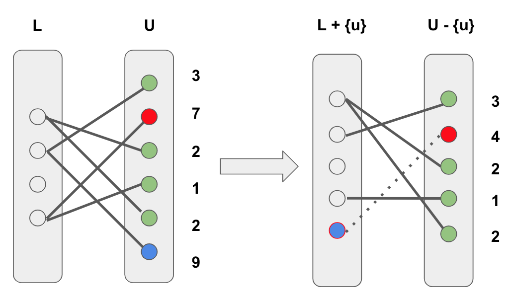
Figure 1: A toy example for our bipartite graph view of active learning. Left: Each unlabeled point has an edge connected to its closest labeled point whose uncertainty is given on the right side. Right: By labeling/moving the bottom point in $U$ to $L$, we directly reduce its uncertainty (from $9$ to $0$) and indirectly reduce the uncertainty of another point (2nd from the top) from $7$ to $4$.

4 Complexity Results

In this section, we first formulate a general version of our bipartite graph optimization problem and establish its complexity. This theoretical analysis guides us in developing approximation algorithms for active learning which will be introduced in Section 5. This section can be skipped on the first reading of the paper.

A bipartite graph $G([U,L],W)$ is a nearest neighbor bipartite graph (or NN-BG) if it satisfies the following two conditions.

• A distance value $d(x,y)\geq 0$ is given for each pair of nodes $x,y$ where $x\in L$ and $y\in U$.

• For each node $y\in U$, $W$ contains exactly one edge $\{x,y\}$, where $x\in L$ is a nearest neighbor of $y$ among all the nodes in $L$ (i.e., for each node $z\in L$, $d(x,y)\leq d(z,y)$).

Thus, in any NN-BG $G([U,L],W)$, each node in $U$ has exactly one edge incident on it; therefore, $|W|=|U|$.

Given an NN-BG $G([U,L],W)$, suppose we move a non-empty subset of nodes $S\subseteq U$ from $U$ to $L$. After this modification, we can find the nearest neighbor for each node $y\in U-S$ and obtain another NN-BG denoted by $G^{\prime}([U-S,L\cup S],W^{\prime})$. We consider the following two problems involving such modifications of NN-BGs.

I. Modification to Minimize the Maximum
Distance (MMMD)

Instance: Given an NN-BG $G([U,L],W)$, an integer $k\leq|U|$ and a non-negative number $\beta$.

Question: Is there a subset $S\subseteq U$ such that (i)  $|S|\leq k$ and (ii)  in the NN-BG $G^{\prime}([U-S,L\cup S],W^{\prime})$, the distance value on each edge $\{x,y\}\in W^{\prime}$ is $\leq$ $\beta$?

II. Modification to Minimize the Total
Distance (MMTD)

Instance: Given an NN-BG $G([U,L],W)$, an integer $k\leq|U|$ and a non-negative number $\sigma$.

Question: Is there a subset $S\subseteq U$ such that (i)  $|S|\leq k$ and (ii)  in the NN-BG $G^{\prime}([U-S,L\cup S],W^{\prime})$, the sum of the distances over all the edges in $W^{\prime}$ is $\leq$ $\sigma$?

We can show that both MMMD and MMTD are NP-complete even when the distance function is a metric. The detailed proofs are shown in the supplementary material.

Theorem 4.1

Problems MMMD and MMTD are NP-complete even when the distance function is a metric.

5 Putting it All Together - Our Algorithms

Here, we first show how to calculate an uncertainty upper bound for each unlabeled point and then translate it as the weight of an edge in the bipartite graph $G([U,L],W)$. Further, we propose two algorithms for sequential and batch-mode active learning, which are different approximation algorithms for the bipartite graph optimization problem. Finally, we extend our active learning strategy for linear regression to polynomial regression, which suits more complex data sets.

5.1 Motivating the Use of $L_{1}$ Distance as an Uncertainty Measure

We now show that the optimum way to calculate the edge weights ($W$) is equivalent to constructing a $L_{1}$ distance measure. Uncertainty sampling is one of the most popular algorithms for active learning in classification [23]. For example, in margin-based methods like SVMs [2] we can calculate the distance between the unlabeled point and the decision boundary as an uncertainty measure. Similarly, in probabilistic models [24], we can calculate the entropy of unlabeled points for uncertainty. Generally speaking, this method computes a measure of the classifier’s uncertainty for each example in the unlabeled set and then returns the most uncertain one. However, the measurement of uncertainty in regression is not as straightforward as for classification problems [16].

We define an intuitive uncertainty measure as follows. Let the data be $d$-dimensional. Suppose the current regression model (learned with ${L}$) predicts for $x$:

$$f(x)=\sum_{i=1}^{d}w_{i}x_{i}+b$$

and the ideal model (learned with $L\cup U$) predicts:

$${f^{*}}(x)=\sum_{i=1}^{d}w_{i}^{*}x_{i}+b^{*}$$

We can rewrite the target value of an arbitrary unlabeled point $x_{u}$ by adding and subtracting the $f$ and $f^{*}$ value for a labeled point $x_{l}$. Note that the positive/negative bias terms ($b$) cancel each other out.

(5.1)

(5.2)

We now attempt to answer the question of which labeled point to use. Here we make a classic machine learning assumption that the model space used matches the data so that $f(x_{l})$ matches $f^{*}(x_{l})$. Now we calculate the approximate error $\delta_{u}$ (due to not having labels for the unlabeled data) for $x_{u}$ as the difference between $f(x_{u})$ in Eq. 5.1 and ${f^{*}}(x_{u})$ in Eq. 5.2:

(5.3) $$\delta_{u}=|{f^{*}}(x_{u})-f(x_{u})|=|\sum_{i=1}^{d}({w}^{*}_{i}-w_{i})(x_{u_{i}}-x_{l_{i}})|$$

We now propose an uncertainty measure $\theta$ for unlabeled point $x_{u}$ and show that $\lambda\theta(x_{u})$ upper bounds $\delta_{u}$ in Theorem 5.1, where $\lambda$ is a constant.

(5.4) $$\theta(x_{u})=\min_{x_{i}\in L}L_{1}(x_{u},x_{i})$$

Eq. 5.4 means the current model’s uncertainty for point $x_{u}$ is based on its nearest labeled point NN$(x_{u})$ measured in $L_{1}$ distance. The following theorem shows the relationship between Eq. 5.3 (an unlabeled point’s estimation error) and Eq. 5.4 (the $L_{1}$ distance between the unlabeled point and its nearest labeled point).

Theorem 5.1

For any unlabeled point $x_{u}$, minimizing $\theta(x_{u})$ is equivalent to minimizing the upper bound of estimation error $\delta_{u}$ for $x_{u}$.

Proof: From equation (5.3) we have $\delta_{u}=|\sum_{i=1}^{d}({w}^{*}_{i}-w_{i})(x_{u_{i}}-x_{l_{i}})|$.

(5.5) $$\begin{split}\delta&=|\sum_{i=1}^{d}({w}^{*}_{i}-w_{i})(x_{u_{i}}-x_{l_{i}})|\\ &\leq\sum_{i=1}^{d}|({w}^{*}_{i}-w_{i})|\times|(x_{u_{i}}-x_{l_{i}})|\\ &\leq\max_{i\in[1,d]}{|{w}^{*}_{i}-w_{i}|}\times\sum_{i=1}^{d}|(x_{u_{i}}-x_{l_{i}})|\\ &=\max_{i\in[1,d]}{|{w}^{*}_{i}-w_{i}|}\times L_{1}(x_{u},x_{l})=\lambda L_{1}(x_{u},x_{l})\\ \end{split}$$

where $\lambda=\max_{i\in[1,d]}|w^{*}_{i}-w_{i}|$ is an unknown constant. Hence, the tightest upper bound for $\delta_{u}$ is achieved when $x_{l}$ is the nearest neighbor of $x_{u}$ in $L_{1}$ measure.

Algorithm 1 Algorithm for Sequential Active Learning

0:   $L$: a set of labeled data ${{\{(x_{i},y_{i})\}}^{l}_{i=1}}$.$U$: a set of unlabeled data ${{\{x_{j}\}}^{n}_{j=l+1}}$.$K$: the total query rounds.

1:  repeat

2:     for each unlabeled $x_{u}$ in $U$ do

3:        for each unlabeled $x_{j}$ in $U$ do

4:           Calculate uncertainty $\theta(x_{j})$ based on Eq. 5.4.

5:           Assume we have selected point $x_{u}$, calculate uncertainty $\theta^{x_{u}}(x_{j})$ based on Eq. 5.4.

6:        end for

7:        Calculate active selection value for $x_{u}$ via Eq. 5.6.

8:     end for

9:     Select $x^{*}$ which maximize $Q$ as Eq. 5.7.

10:     Retrain the model with $(L\cup(x^{*},y^{*}))$ and evaluate the model on the hold-out test set.

11:  until Query round number reaches $K$.

5.2 Proposed Active Selection Strategy for Sequential Query

We now propose an evaluation function $Q$ for active selection which chooses to query one point at each round. We first calculate the current uncertainty for each unlabeled point $x_{i}\in U$ as $\theta(x_{i})$ based on Eq. 5.4. We then calculate the uncertainty for each unlabeled point if $x_{u}$ had been queried, which we refer to as ${\theta^{x_{u}}}(x_{i})$. Next, we calculate the reduction of uncertainty for each unlabeled point as $\theta(x_{i})-{\theta^{x_{u}}}(x_{i})$. Finally we calculate the difference between the graphs defined in Section 3 after querying $x_{u}$ as:

(5.6) $$Q(x_{u})=\sum_{i\in U}\theta(x_{i})-\sum_{j\in U^{{}^{\prime}}}\theta^{x_{u}}(x_{j}),$$

where $U^{{}^{\prime}}=U-\{x_{u}\}$. Now we select the point which maximizes the differences as $x^{*}$:

(5.7) $$x^{*}=\operatorname*{arg\,max}_{x_{u}}{Q}(x_{u})$$

The pseudocode for our proposed algorithm is summarized in Algorithm 1. At each iteration of active learning, our algorithm selects a point $x^{*}$ which maximizes our active selection function. After that, we retrain our model and test the newly trained model with the hold-out test set. The whole process is repeated until the number of querying rounds reaches the chosen maximum value. To speed up our proposed algorithm, the outer loop’s computations in Algorithm 1 can be run in parallel so the total time complexity for one query can be reduced to $O(|U|*|L|)$.

Algorithm 2 Algorithm for Batch Active Learning

0:   $L$: a set of labeled data ${{\{(x_{i},y_{i})\}}^{l}_{i=1}}$.$U$: a set of unlabeled data ${{\{x_{j}\}}^{n}_{j=l+1}}$.$K$: the total query points in a batch. $S$: the initial query set created by running Algorithm 1 for $K$ rounds.

1:  repeat

2:     for each unlabeled $x_{u}$ in $U-S$ do

3:        for each labeled $x_{l}$ in $S$ do

4:           Based on Eq. 5.6, we now calculate the reduction for a set of points $S$ rather than a single point.

5:           Calculate the total uncertainty reduction $Q(S)$.

6:           $S^{{}^{\prime}}=S-\{x_{l}\}+\{x_{u}\}$

7:           Calculate the total uncertainty reduction $Q(S^{{}^{\prime}})$.

8:           if $Q(S)<Q(S^{{}^{\prime}})$ then

9:              $S=S^{{}^{\prime}}$

10:           end if

11:        end for

12:     end for

13:  until $\forall S^{{}^{\prime}}$ $Q(S)>Q(S^{{}^{\prime}})$.

14:  Output final query batch $S$.

5.3 Proposed Active Selection Strategy for Batch Mode Query

Most active learning methods have focused on sequential active learning which selects a single point to query in each iteration. In this setting, the model has to be retrained after each new example is queried and is not a realistic setting. (Multiple experts annotate data in a parallel labeling system.) Moreover, using our sequential active learning method to optimize the overall uncertainty reduction in the bipartite graph is less accurate than optimizing a group of points. We will demonstrate the performance advantage of batch mode query in Section 6.

Our goal for batch mode query is to select a batch of $K$ data points $S_{u}$ that provides the largest overall uncertainty reduction. Searching for an optimal solution will be computationally expensive (as suggested by the hardness results in Section 3). To reduce the computation overhead, we propose to use a local search approximation algorithm to optimize the batch mode query problem.

The local search algorithm [25] with a single swap is a popular algorithm for $k$-Median problem. We apply this idea to our active learning strategy. Let the batch size be $K$. We choose an initial set of $K$ query points using our sequential active learning method (Algorithm 1). We then repeatedly check the unlabeled points in the pool and swap them with the $K$ query points if the newly added point can reduce the total uncertainty reduction. Reference [25] proved that local search with $p$ swaps is a $3+2/p$ approximation algorithm, which gives an approximation ratio of $5$ in the single swap case with linear runtime. The pseudocode for the batch mode query algorithm is summarized in Algorithm 2.

5.4 Extension to Other Forms of Regression

Linear regression is popular for many real-world applications due to its simplicity and interpretability. So far, we have discussed sequential and batch mode query strategies for linear regression. However, it suffers from overfitting problem and does not generalize well to complex data sets. In this section, we show how our current formulation can be extended to other forms of regression. To fit complex data, one common approach within machine learning is to use linear models trained on non-linear functions of the data. This approach maintains the generally fast performance and high interpretability of linear models while allowing them to fit a much wider range of data.

Let an instance $x$ with $d$ dimensions have the coordinates $[x_{1},x_{2},...x_{d}]$. We construct the $k$-order polynomial features for $x$ by using the multinomial theorem. Thus we have polynomial features like $x_{i}^{k}$ and interaction terms like $x_{i}*x_{j}^{k-1}$. A toy example for second-order polynomial features with interaction terms for two dimensional data is as follows: given the original data as: $x=[x_{1},x_{2}]$, the new feature is: $z=[x_{1},x_{2},x_{1}x_{2},x_{1}^{2},x_{2}^{2}]$ and the new regression model is: $f(z)=w_{0}+w_{1}z_{1}+w_{2}z_{2}+w_{3}z_{3}+w_{4}z_{4}+w_{5}z_{5}$.

To prevent overfitting, we also impose the regularization term to polynomial regression as ridge regression. By considering linear fits within a higher-dimensional space built with these basis functions, the model can be used for a much boarder range of data. We also tested our approach for ridge regression. Due to limited space, our experimental results for ridge regression appear in the supplementary material.

6 Experiments

Here we aim to demonstrate the effectiveness of our approach empirically. In particular, we address the following three questions.

• How do our results compare with baseline active learning methods for linear regression? This directly tests the tightness of our bound (Theorem 5.1).

• How does our proposed method perform when the query results are noisy?

• How does our proposed method perform on different forms of regression?

The first and second questions test the usefulness of our proposed algorithms in practice while the last question addresses the effectiveness of applying our proposed method to other forms of regressions.

To compare the effectiveness of our proposed methods and answer the above questions, our algorithms are compared with four representative baselines.

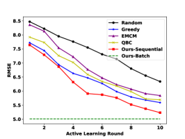
(a) Housing

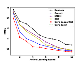
(b) Concrete

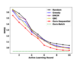
(c) Yacht

(d) PM10

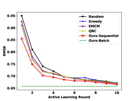
(e) Redwine

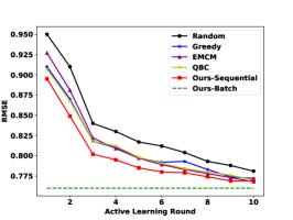
(f) Whitewine

Figure 2: Comparison results for the benchmark data sets with linear regression, (a) to (f) are learned with exact labels. Results are averaged over 30 random trials with ranking results shown in Table 2.

• Random: Randomly select an instance from the unlabeled pool, which is widely used as active learning baseline.

• Greedy passive sampling [16]: This approach will select an instance from the unlabeled pool which has the largest minimum Euclidean distance from the labeled set in feature space.

• Query by committee algorithm [8]: This algorithm selects an instance that has the largest variance among the committee’s prediction. The committee is constructed on bootstrap examples, and the number of committee members is set to be $4$.

• Expected model change maximization [10]: This algorithm quantifies the change as the difference between the current model parameters and the new model parameters, and chooses an unlabeled instance which results in the greatest change.

For all the baselines, we use the same parameters in original papers. For simplicity, we use Random, Greedy, QBC, and EMCM to denote the above baselines; our sequential query method is denoted as Ours-Sequential, our batch query method is denoted as Ours-Batch.

Table 1: Statistics and of Classical Experimental Data Sets Used in Active Regression (see [16] [10]).

Data sets	# instances	# features	Source
Housing	506	13	UCI
Concrete	1030	8	UCI
Yacht	308	6	UCI
PM10	500	7	StatLib
Redwine	1599	11	UCI
Whitewine	4898	11	UCI

Data Description. We used six benchmark data sets which are chosen from the UCI machine learning repository [26] and CMU’s StatLib [27]: Housing, Concrete, Yacht, PM10, Redwine, Whitewine. These data sets were collected from various domains and have been extensively used for testing regression models. Their statistics and descriptions are shown in Table 1.

Experimental Configuration. For each dataset, 1% of the instances are sampled to initialize the labeled set $L$. We use minimal initial data set to demonstrate the advantages of our proposed algorithm. For evaluating the regression model for each run, 30% of the instances are held out as the test set; the rest of the instances are used for active learning. For each run we will query $20\%$ of the unlabeled instances. Note that we did not query all the unlabeled instances because the performances of most methods converge after some queries. In our plots we use query round as our x-axis; round one means $2\%$, round two means $4\%$ of the unlabeled instances and so on; we have $10$ rounds in total. For the batch mode query, we will directly choose a single batch consisting of all $20\%$ points to query.

We report the average results over the $30$ runs of experiments. For the features in each dataset, we normalize the features using the standard score function (Z-score): $z=\frac{x-\mu}{\sigma}$ where $\mu$ is the mean of the population and $\sigma$ is the standard deviation of the population. To simulate the noisy annotations setting, we first calculate the standard deviation of the current labels as $std(y)$ and then add a Gaussian noise $N(0,0.1*std(y))$ for each newly added query point.

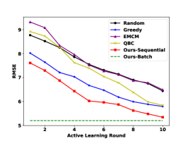
(a) Housing^∗

(b) Concrete^∗

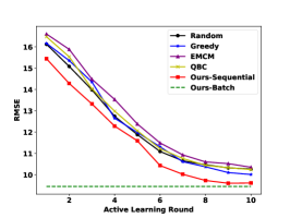
(c) Yacht^∗

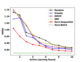
(d) PM10^∗

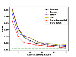
(e) Redwine^∗

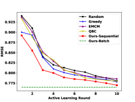
(f) Whitewine^∗

Figure 3: Comparison results for the benchmark data sets with linear regression, (a) to (f) are learned with noisy labels. Results are averaged over 30 random trials.

Results for Non-Noisy Setting. Figure 2 plots the RMSE (Root Mean Squared Error) curves against the total number of queries for all the compared approaches. We first discuss the noise-free results in parts (a) to (f) of Figure 2. Generally speaking, active learning methods usually achieve lower RMSE than the Random method. As can be seen from the plots, both QBC and EMCM perform better than Random and their performances are close to each other. This is reasonable because their ideas are similar; QBC builds a committee to find the unlabeled point which has the largest prediction variance while EMCM builds an ensemble to find the instance which causes the largest changes in the model’s parameters.

EMCM method tends to fluctuate at the beginning of the training since its optimization objective only looks for unlabeled instances that can bring the largest model change, regardless of the the direction of change. Greedy sampling can achieve decent performance in some of the data sets, but its performance is not consistent; a possible reason is that different distributions of the labeled and unlabeled data could fool the greedy method into querying some outliers. Our proposed sequential query approach consistently achieves lower RMSE than other methods in most cases.

For the batch-mode query, one can see querying a batch is always better than our sequential greedy query across all the data sets. This result is expected since the local search approximation algorithm reduces more in terms of the overall uncertainty for unlabeled points. The better performance of batch mode query also reflects that optimizing the overall uncertainty upper bound is useful in practice. We haven’t made comparisons to model-based batch query algorithms since their performance will worse compared to their sequential query versions. For example, batch-EMCM performs worse than sequential EMCM in [15]; this is because the model is updated after each new example is chosen and added to the training set so that each example is selected with more information.

Results for Noisy Setting. Parts (a) to (f) of Figure 3 show the RMSE curves with noisy annotations. Both QBC and EMCM perform worse than in the noise-free setting (see Figure 2). This result is expected because we introduce Gaussian noise into each active query’s feedback which harms the performance of the model-based methods. Both QBC and EMCM assume the labels are noise-free and depend highly on the quality of learned functions. The greedy method still performs inconsistently, but it is less vulnerable to the noise because it uses feature-based sampling strategy. Furthermore, our proposed approach achieves lower average RMSE in a noisy setting. This is to be expected as our method does not directly depend on the regression function.

Table 2: First place/second place/others counts of our method on linear regression versus the baselines with varied numbers of queries. The number of queries is represented by the percentage of the unlabeled data. Each method is repeated for $30$ runs.

	Number of queries
	5%	10%	15%	20%
Housing	18/8/4	18/9/3	18/10/2	18/10/2
Concrete	18/9/3	19/9/2	20/9/1	20/9/1
Yacht	18/9/3	18/10/2	18/10/2	18/10/2
PM10	15/12/3	14/13/3	14/13/3	14/13/3
Redwine	14/11/5	14/11/5	15/10/5	15/10/5
Whitewine	17/10/3	17/10/3	18/9/3	18/9/3
All	100/59/21	100/62/18	103/61/16	103/61/16

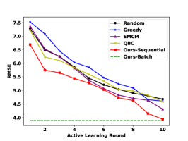
(a) Housing

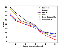
(b) Concrete

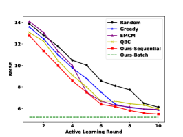
(c) Yacht

Figure 4: Comparison results for the three harder (based on RMSE) data sets with polynomial regression.

The overall performance of our sequential query method for linear regression, shown in Table 2, summarizes the ranking counts of our method versus the other methods based on the noise-free setting. Note that an active learning algorithm’s performance varies with the distributions of initial labeled and unlabeled points. Thus, our method performs best in more than half of the tests and behaves consistently as the number of queries is increased. Significantly, this shows that our method does not only performs better on average, but it also consistently outperforms the competitors.

Active Learning Experiments on Different Forms of Regression. We evaluated our extension for ridge regression and the results are in line with the linear regression results. The details are summarized in the supplementary material. To adapt to complex data, we discuss experiments for polynomial regression in this section. We chose three datasets, namely Housing, Concrete, and Yacht. The reason for selecting them is that the performance of linear regression for these datasets is not good enough. Figure 4 plots the RMSE curves for polynomial regression. We set the default regularization parameter as $1$ across all the data sets.

Compared to linear regression results in Figure 2, we find that polynomial regression works much better on these three datasets with a much lower RMSE. Greedy behaves in a more unstable manner; it achieves decent performance for Concrete and Yacht datasets but loses to Random for the Housing dataset. This is possible because with larger feature dimensions, Greedy is more likely to pick some outliers which are less informative. The EMCM and QBC methods perform similarly across all data sets. They perform worse at the beginning and gradually become better with an increase in the number of labeled points. Our proposed method performs consistently better than the baseline methods, especially in the first $5$ active learning rounds.

7 Conclusions

We propose a new graph-based approach for active learning in regression. We formulate the active learning problem as a bipartite graph optimization problem to maximize the overall reduction in uncertainty caused by moving points from the unlabeled collection to the labeled collection. Experimental results on benchmark data show that the proposed approach can efficiently find valuable points to improve the active learning method. We explored both sequential and batch mode learning. Experimental results show that the proposed measure of uncertainty and the method achieve promising results for different forms of regression. A limitation of our method is the high computational overhead due to searching instances’ neighbors in each active learning round. In future work, we propose to speed up our algorithms by using more efficient data structures such as KD-trees and advanced hashing methods [5, 6]. Such techniques will enable us to apply our approach to large-scale regression tasks.

References

- [1] D. A. Cohn, Z. Ghahramani, and M. I. Jordan, “Active learning with statistical models,” JAIR, 1996.
- [2] S. Tong and D. Koller, “Support vector machine active learning with applications to text classification,” JMLR, 2001.
- [3] H. T. Nguyen and A. Smeulders, “Active learning using pre-clustering,” in ICML, 2004.
- [4] S. Dasgupta and D. Hsu, “Hierarchical sampling for active learning,” in ICML, 2008.
- [5] B. Qian, X. Wang, J. Wang, H. Li, N. Cao, W. Zhi, and I. Davidson, “Fast pairwise query selection for large-scale active learning to rank,” in ICDM, 2013.
- [6] S. Gilpin, B. Qian, and I. Davidson, “Efficient hierarchical clustering of large high dimensional datasets,” in CIKM, 2013.
- [7] S.-J. Huang, R. Jin, and Z.-H. Zhou, “Active learning by querying informative and representative examples,” TPAMI, 2014.
- [8] R. Burbidge, J. J. Rowland, and R. D. King, “Active learning for regression based on query by committee,” in IDEAL, 2007.
- [9] M. Sugiyama and S. Nakajima, “Pool-based active learning in approximate linear regression,” Machine Learning, vol. 75, no. 3, pp. 249–274, 2009.
- [10] W. Cai, Y. Zhang, and J. Zhou, “Maximizing expected model change for active learning in regression,” in ICDM, 2013.
- [11] S. Sabato and R. Munos, “Active regression by stratification,” in NIPS, 2014.
- [12] C. Riquelme, R. Johari, and B. Zhang, “Online active linear regression via thresholding,” in AAAI, 2017.
- [13] L. Malago, N. Cesa-Bianchi, and J. Renders, “Online active learning with strong and weak annotators,” in NIPS Workshop on Learning from the Wisdom of Crowds, 2014.
- [14] C. Zhang and K. Chaudhuri, “Active learning from weak and strong labelers,” in NIPS, 2015.
- [15] W. Cai, M. Zhang, and Y. Zhang, “Batch mode active learning for regression with expected model change,” IEEE Transactions on Neural Networks and Learning Systems, vol. 28, no. 7, pp. 1668–1681, 2016.
- [16] H. Yu and S. Kim, “Passive sampling for regression,” in ICDM, IEEE, 2010.
- [17] K. Yu, J. Bi, and V. Tresp, “Active learning via transductive experimental design,” in ICML, 2006.
- [18] R. Chattopadhyay, Z. Wang, W. Fan, I. Davidson, S. Panchanathan, and J. Ye, “Batch mode active sampling based on marginal probability distribution matching,” TKDD, 2013.
- [19] Z. Wang and J. Ye, “Querying discriminative and representative samples for batch mode active learning,” TKDD, 2015.
- [20] Y. Yan, R. Rosales, G. Fung, and J. G. Dy, “Active learning from crowds.,” in ICML, 2011.
- [21] S.-J. Huang, J.-L. Chen, X. Mu, and Z.-H. Zhou, “Cost-effective active learning from diverse labelers.,” in IJCAI, 2017.
- [22] M. R. Gary and D. S. Johnson, “Computers and intractability: A guide to the theory of np-completeness,” 1979.
- [23] B. Settles, “Active learning,” Synthesis Lectures on Artificial Intelligence and Machine Learning, 2012.
- [24] B. Settles, M. Craven, and S. Ray, “Multiple-instance active learning,” in NIPS, 2008.
- [25] V. Arya, N. Garg, R. Khandekar, A. Meyerson, K. Munagala, and V. Pandit, “Local search heuristics for k-median and facility location problems,” SIAM Journal on Computing, vol. 33, no. 3, pp. 544–562, 2004.
- [26] K. Bache and M. Lichman, “UCI machine learning repository,” 2013.
- [27] P. Vlachos, “StatLib project repository,” Carnegie Mellon University, 2000.