The VANDELS survey: A strong correlation between Ly$\alpha$ equivalent width and stellar metallicity at $\mathbf{3\leq z\leq 5}$

Abstract

We present the results of a new study investigating the relationship between observed Ly$\alpha$ equivalent width ($W_{\lambda}$(Ly$\alpha$)) and the metallicity of the ionizing stellar population ( $Z_{\star}$) for a sample of $768$ star-forming galaxies at $3\leq z\leq 5$ drawn from the VANDELS survey. Dividing our sample into quartiles of rest-frame $W_{\lambda}$(Ly$\alpha$) across the range $-58\rm{\AA}\lesssim$ $W_{\lambda}$(Ly$\alpha$) $\lesssim 110\rm{\AA}$ we determine  $Z_{\star}$ from full spectral fitting of composite far-ultraviolet (FUV) spectra and find a clear anti-correlation between $W_{\lambda}$(Ly$\alpha$) and  $Z_{\star}$. Our results indicate that  $Z_{\star}$ decreases by a factor $\gtrsim 3$ between the lowest $W_{\lambda}$(Ly$\alpha$) quartile ($\langle$$W_{\lambda}$(Ly$\alpha$)$\rangle=-18\rm{\AA}$) and the highest $W_{\lambda}$(Ly$\alpha$) quartile ($\langle$$W_{\lambda}$(Ly$\alpha$)$\rangle=24\rm{\AA}$). Similarly, galaxies typically defined as Lyman Alpha Emitters (LAEs; $W_{\lambda}$(Ly$\alpha$) $>20\rm{\AA}$) are, on average, metal poor with respect to the non-LAE galaxy population ($W_{\lambda}$(Ly$\alpha$) $\leq 20\rm{\AA}$) with  $Z_{\star}$${}_{\rm{non-LAE}}\gtrsim 2\times$  $Z_{\star}$_LAE. Finally, based on the best-fitting stellar models, we estimate that the increasing strength of the stellar ionizing spectrum towards lower  $Z_{\star}$ is responsible for $\simeq 15-25\%$ of the observed variation in $W_{\lambda}$(Ly$\alpha$) across our sample, with the remaining contribution ($\simeq 75-85\%$) being due to a decrease in the H i/dust covering fractions in low  $Z_{\star}$ galaxies.

1 Introduction

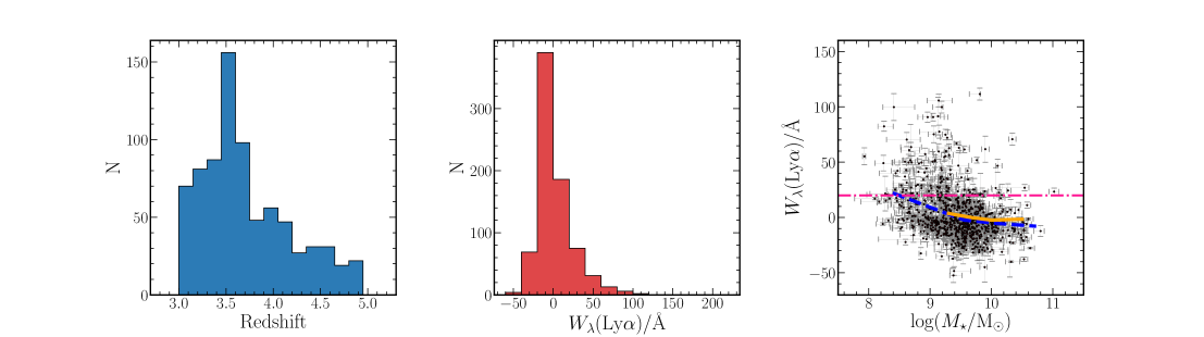
Figure 1: Left-hand panel: Redshift distribution of the $768$ galaxies in our final sample. The redshift range is $3.0\leq z\leq 5.0$ with a median redshift of $z_{\rm{median}}=3.60$. Central panel: The distribution of rest-frame Ly$\alpha$ equivalent widths; the $W_{\lambda}$(Ly$\alpha$) values fall within the range $-58\rm{\AA}\lesssim$ $W_{\lambda}$(Ly$\alpha$) $\lesssim 110\rm{\AA}$ with a median value of $W_{\lambda}$(Ly$\alpha$) $\simeq-4\rm{\AA}$. Right-hand panel: The relationship between galaxy stellar mass and $W_{\lambda}$(Ly$\alpha$) for our sample. The circular data points with error bars are the individual galaxies with the blue dashed curve showing a running average of the data. The solid yellow curve shows the $z\simeq 3$ log($M_{\ast}$/M_⊙)$-$ $W_{\lambda}$(Ly$\alpha$) relation derived by Du et al. (2018) for comparison. The pink dot-dashed line illustrates an equivalent width cut-off commonly used to classify galaxies as LAEs ($W_{\lambda}$(Ly$\alpha$)$>20\rm{\AA}$); based on this definition $83\%$ of the LAEs in our sample have log($M_{\ast}$/M_⊙)$\leq 9.5$, highlighting the fact that Ly$\alpha$ emission becomes more prevalent at lower stellar masses.

The Ly$\alpha$ emission line remains a powerful tool for determining the nature of ionizing sources within galaxies as well as probing the ionization state and covering fraction of their interstellar and/or circumgalactic H i gas and dust. In addition, since Ly$\alpha$ emission appears to be intrinsically linked to the escape fraction of Lyman continuum (LyC) photons (e.g. Nestor et al., 2013; Verhamme et al., 2017; Steidel et al., 2018; Marchi et al., 2018), understanding the nature of Ly$\alpha$ emitting galaxies will be crucial in characterizing the galaxy population responsible for reionization at $z\gtrsim 6$ (Fontanot et al., 2014; Robertson et al., 2015).

The observability of Ly$\alpha$ depends on the production rate of Ly$\alpha$ photons within galaxies and on the probability that those photons can escape without being absorbed and/or scattered by the surrounding gas and dust (Dijkstra, 2014). Over the past two decades it has become clear that the strength of Ly$\alpha$ emission increases towards lower mass, relatively dust-free galaxies (Kornei et al., 2010; Hayes et al., 2014; Cassata et al., 2015; Hathi et al., 2016; Oyarzún et al., 2017; Marchi et al., 2019). These galaxies typically have low covering fractions of H i gas as inferred from weak Lyman series or low-ionization metal line absorption in their rest-frame UV spectra (e.g. Shapley et al., 2003; Du et al., 2018; Trainor et al., 2019). Furthermore, for galaxies with large rest-frame equivalent widths ($W_{\lambda}$(Ly$\alpha$)), the peak of the Ly$\alpha$ emission is observed to be closer to a galaxy’s systemic redshift, again highlighting the fact that Ly$\alpha$ emission is favoured when the H i opacity in the immediate vicinity of the galaxy is low (Erb et al., 2014; Trainor et al., 2015). In general, these probes of opacity favour higher Ly$\alpha$ escape fractions in low-mass galaxies.

More recently, signatures of the intrinsic production rate of Ly$\alpha$ photons have also been explored. Using tracers primarily based on rest-frame optical emission-line ratios, various studies have shown that $W_{\lambda}$(Ly$\alpha$) is larger in galaxies containing low-metallicity, high-excitation, H ii regions powered by stellar populations that emitting a harder ionizing continuum. Galaxies selected via line ratios indicative of highly-ionized gas (e.g. [O iii]/[O ii], [O iii]/H $\beta$) typically exhibit stronger Ly$\alpha$ emission than the general population (Erb et al., 2016; Trainor et al., 2016, 2019). Moreover, gas-phase metallicity ( $Z_{\rm{g}}$) estimates of Ly$\alpha$ emitters (LAEs) indicate that they are metal-poor with respect to non-LAEs of similar stellar mass and star-formation rate (Charlot & Fall, 1993; Finkelstein et al., 2011; Nakajima et al., 2013; Song et al., 2014; Du et al., 2019). Of course, it is likely that the physical processes governing Ly$\alpha$ production and escape are fundamentally linked. For example, we would expect young, low-metallicity, stellar populations that emit harder ionizing spectra to be more effective at ionizing gas in their immediate vicinity, thereby reducing the covering fraction of H i and aiding the escape of Ly$\alpha$ photons (e.g. Erb et al., 2010; Heckman et al., 2011; Law et al., 2012; Erb et al., 2014). In other words, those galaxies that produce Ly$\alpha$ photons most efficiently should also be the ones from which those photons have the highest likelihood of escape.

Based on this picture, we expect to observe a correlation between $W_{\lambda}$(Ly$\alpha$) and the stellar metallicity ( $Z_{\star}$) of the ionizing population. Although existing measurements of  $Z_{\rm{g}}$ strongly hint at such an association, the correlation between  $Z_{\rm{g}}$ and $W_{\lambda}$(Ly$\alpha$) still suffers from various systematics associated with determining  $Z_{\rm{g}}$, which become especially severe in the highly-ionized H ii regions typical of $z\gtrsim 2$ Ly$\alpha$ emitters, where locally-calibrated line ratio diagnostics may not be applicable (Kewley et al., 2013; Cullen et al., 2014; Steidel et al., 2014; Kewley et al., 2019). In principle, a cleaner estimate of the metallicity dependence can be made with  $Z_{\star}$, although to date this has never been demonstrated explicitly. In a recent paper we showed how  $Z_{\star}$ of the young, hot, O- and B-type stellar populations in high-redshift galaxies can be estimated from rest-frame far-ultraviolet (FUV) spectra using a sample of star-forming galaxies at $2.5<z<5.0$ from the VANDELS survey (Cullen et al., 2019). Using this approach, it should be possible to investigate the connection between $W_{\lambda}$(Ly$\alpha$) and  $Z_{\star}$ and provide a new and powerful constraint on the nature of Ly$\alpha$ emitting galaxies.

In this paper, we focus on a subset of VANDELS galaxies with spectral coverage of the Ly$\alpha$ line to investigate, for the first time, the relationship between $W_{\lambda}$(Ly$\alpha$) and  $Z_{\star}$. In Section 2 we describe our $z\gtrsim 3$ VANDELS star-forming galaxy sample and our method for determining $W_{\lambda}$(Ly$\alpha$). Our determination of the $W_{\lambda}$(Ly$\alpha$) $-$  $Z_{\star}$ relation is presented in Section 3 and the implications are discussed in Section 4. Finally, we list our main conclusions in Section 5. Throughout the paper all metallicities are quoted relative to the solar abundance taken from Asplund et al. (2009), which has a bulk composition by mass of $Z_{\ast}=0.0142$, and all equivalent width values are quoted in the rest-frame with positive values corresponding to emission and negative values to absorption. We assume the following cosmology: $\Omega_{M}=0.3$, $\Omega_{\Lambda}=0.7$, $H_{0}=70$ km s^-1 Mpc^-1.

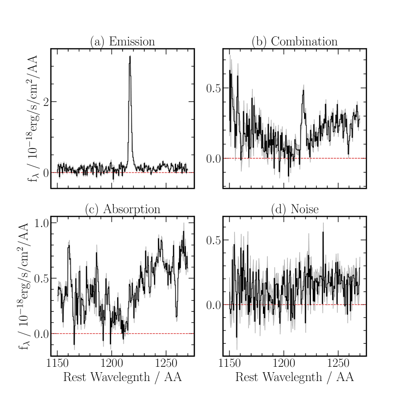
Figure 2: Example spectra illustrating each of the four Ly$\alpha$ morphological classifications: emission, combination, absorption and noise. For each classification, $W_{\lambda}$(Ly$\alpha$) was calculated following the methods outlined in Kornei et al. (2010).

2 Data and Sample Selection

The spectroscopic data used in this work were obtained as part of the VANDELS ESO public spectroscopic survey (McLure et al., 2018; Pentericci et al., 2018). VANDELS is a deep, optical, spectroscopic survey of the CANDELS (Grogin et al., 2011; Koekemoer et al., 2011) CDFS and UDS fields with the ESO-VLT VIMOS spectrograph on ESO’s Very Large Telescope (VLT), targeting massive passive galaxies at $1.0\leq z\leq 2.5$, bright star-forming galaxies at $2.4\leq z\leq 5.5$ and fainter star-forming galaxies at $3.0\leq z\leq 7.0$. VIMOS observations were obtained using the medium-resolution grism which covers the wavelength range $4800<\lambda_{\rm{obs}}<10000\rm{\AA}$ with a resolution of $R=580$ and a dispersion of 2.5 Å per pixel. The observations and reduction of the VIMOS spectra are described in detail in the first VANDELS data release paper (Pentericci et al., 2018).

The sample utilized here is drawn from the third VANDELS data release (DR3). Redshifts for all of the spectra have been determined by members of the VANDELS team and assigned a redshift quality flag ($z_{\rm{flag}}$) as described in Pentericci et al. (2018). In this work, we focus exclusively on star-forming galaxies at $3\leq z\leq 5$ to ensure both coverage of the Ly$\alpha$ emission/absorption feature and to enable robust determination of stellar metallicities (Cullen et al., 2019). All galaxies are required to have a redshift quality flag of $z_{\rm{flag}}=3,4$ or $9$ (corresponding to a $\geq 95\%$ probability of being correct). In total, $777$ galaxies in DR3 satisfy these criteria. We derived stellar masses for our Ly$\alpha$ sample using fast++, a rewrite of fast (Kriek et al., 2009) described in Schreiber et al. (2018). We employed the Bruzual & Charlot (2003) stellar population synthesis models assuming a Chabrier (2003) IMF and delayed exponentially-declining star-formation histories ($M_{\ast}\propto te^{-t/\tau}$) where $t$ is the time since the onset of star formation and $\tau$ is the characteristic star formation timescale. The age was varied between $7.7<\mathrm{log}(t/\mathrm{yr})<10.1$ in steps of $\Delta(\mathrm{log}(t/\mathrm{yr}))=0.1$, and the star formation timescale was varied between $8.0<\mathrm{log}(\tau/\mathrm{yr})<10.0$ in steps of $\Delta(\mathrm{log}(\tau/\mathrm{yr}))=0.2$. Dust attenuation was described using the Calzetti et al. (2000) attenuation law with $A_{\rm{V}}$ in the range $0.0\leq A_{\rm{V}}\leq 5.0$ and the stellar population metallicity was allowed to vary between $0.3-2.5\times\mathrm{Z}_{\odot}$. The stellar masses of the galaxies in our sample range from $10^{8}-10^{11}\mathrm{M}_{\odot}$ with a median value of $3\times 10^{9}\mathrm{M}_{\odot}$; the median redshift of the sample is $z_{\rm{median}}=3.60$. The redshift distribution is illustrated in Fig. 1.

2.1 Measuring Ly$\alpha$ equivalent widths

To estimate $W_{\lambda}$(Ly$\alpha$) for each galaxy we followed the method described in Kornei et al. (2010) (K10). This technique is designed to provide a robust determination of the wavelength range over which the flux should be integrated based on the morphology of the Ly$\alpha$ line. Individual galaxies were visually classified as either ‘emission’, ‘absorption’, ‘combination’ or ‘noise’ (Fig. 2; see K10 for a detailed description of the various classifications). In the first three cases, the peak of the emission/absorption is located and the upper and lower wavelength limits for the flux integration are defined as the wavelength values either side of the peak where the flux intersects an average continuum level. The blue (i.e. lower) continuum ($c_{\rm{blue}}$) is defined as the median flux value in the range $1120\rm{\AA}<\lambda_{\rm{rest}}<1180\rm{\AA}$ and the red continuum ($c_{\rm{red}}$) as the median value in the range $1228\rm{\AA}<\lambda_{\rm{rest}}<1255\rm{\AA}$. In the case of ‘absorption’ and ‘combination’ sources, the spectra are first smoothed with a boxcar function of width 6 pixels ($\simeq 3.5\rm{\AA}$ rest-frame) to minimize the possibility of noise spikes affecting the determination of the upper and lower wavelength boundaries. For ‘noise’ sources, the Ly$\alpha$ flux is simply defined as the integrated flux in the range $1200\rm{\AA}<\lambda_{\rm{rest}}<1228\rm{\AA}$. In all cases the Ly$\alpha$ line flux is divided by $c_{\rm{red}}$ to yield $W_{\lambda}$(Ly$\alpha$). For $10/777$ objects $c_{\rm{red}}$ was detected at $\leq 2\sigma$ in the spectrum; in these cases $c_{\rm{red}}$ was estimated using the best fitting SED from the fast++ photometric fits. For each object, this process was repeated 500 times, each time perturbing the flux value in each pixel using its estimated error. The value of $W_{\lambda}$(Ly$\alpha$) was taken as the median value of the resulting distribution and the error was estimated using the median absolution deviation (MAD) of the distribution, where $\sigma\simeq 1.4826\times\mathrm{MAD}$.

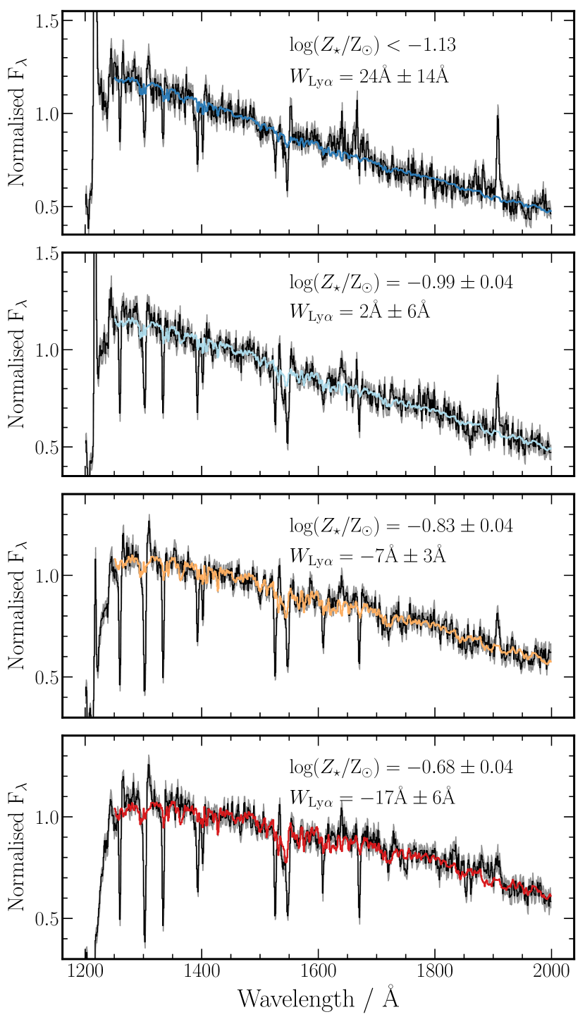
Figure 3: Composite spectra in four independent $W_{\lambda}$(Ly$\alpha$) quartiles (black lines) with the best-fitting Starburst99 WM-Basic SPS model over-plotted. In each panel the median and standard deviation of $W_{\lambda}$(Ly$\alpha$) within the quartile is indicated, along with the best-fitting value of log($Z_{\ast}$/Z_⊙) and its $1\sigma$ (statistical) error.

Table 1: Physical properties and line equivalent widths for the $W_{\lambda}$(Ly$\alpha$) quartiles

Quartile	$W_{\lambda}$(Ly$\alpha$) (individual)a	$W_{\lambda}$(Ly$\alpha$)(composite)b	$W_{\lambda}$(C iii])b	log($M_{\ast}$/M⊙)a	log($Z_{\ast}$/Z⊙)	$\beta^{c}$
Q1	$23.68\pm 12.69$	$19.41\pm 0.78$	$2.89\pm 0.23$	$9.18\pm 0.47$	$<1.08$ $(68\%)$	$-1.99\pm 0.02$
Q2	$2.04\pm 6.14$	$3.76\pm 0.22$	$1.53\pm 0.24$	$9.45\pm 0.47$	$-0.98\pm 0.04$	$-1.75\pm 0.02$
Q3	$-7.30\pm 3.02$	$-4.61\pm 0.21$	$1.22\pm 0.16$	$9.54\pm 0.44$	$-0.82\pm 0.04$	$-1.34\pm 0.02$
Q4	$-17.69\pm 6.12$	$-18.82\pm 0.18$	$0.84\pm 0.37$	$9.59\pm 0.31$	$-0.69\pm 0.04$	$-1.14\pm 0.02$
a The median and standard deviation (estimated as $\sigma\simeq 1.4826\times\mathrm{MAD}$) for the individual galaxies in each quartile.
b Equivalent width values and their associated errors measured directly from the composite spectra.
c UV continuum slope measured directly from the composite spectra following the method described in Cullen et al. (2017).

There were $8$ objects for which $W_{\lambda}$(Ly$\alpha$) could not be estimated due to strong contamination at the location of the Ly$\alpha$ line. One further object had a extreme equivalent width value of $>2000\rm{\AA}$; this object was undetected in the continuum and potentially contaminated by a secondary object in the slit. These $9$ objects were removed from the sample leaving a total of $768$ galaxies. Of these, $239/768$ objects were classified as emission spectra, $355/768$ as absorption, $64/768$ as combination and $110/768$ as noise. The resulting rest-frame equivalent widths span the range $-52\rm{\AA}\lesssim$ $W_{\lambda}$(Ly$\alpha$) $\lesssim 112\rm{\AA}$ with a median value of $W_{\lambda}$(Ly$\alpha$) $=-3.6\rm{\AA}$ as shown in Fig. 1. We note that this median value is slightly lower than the median $W_{\lambda}$(Ly$\alpha$) determined for Lyman Break Galaxy (LBG) selected samples at similar redshifts (c.f. $4\rm{\AA}$, Kornei et al., 2010) which is a result of LBG selection criteria being biased towards bluer galaxies that exhibit, on average, stronger Ly$\alpha$ emission (see Section 4).

Fig. 1 also shows the relation between $W_{\lambda}$(Ly$\alpha$) and stellar mass for the galaxies in our sample. Consistent with results reported elsewhere in the literature (e.g. Oyarzún et al., 2016; Du et al., 2018; Marchi et al., 2019), we find a mild anti-correlation such that the average $W_{\lambda}$(Ly$\alpha$) is increasing towards lower stellar-mass galaxies. We note that this trend should not be a result of observational biases since, by design, the median continuum signal-to-noise ratio (SNR) of the VANDELS spectra is approximately constant as a function of stellar mass (McLure et al., 2018). Therefore, we are not biased against low- $M_{\star}$, low-$W_{\lambda}$(Ly$\alpha$) objects (i.e. objects that would lie in the bottom left-hand corner of the rightmost panel in Fig. 1). In the following section we will return to a discussion of the $W_{\lambda}$(Ly$\alpha$)- $M_{\star}$ correlation.

3 Analysis

Armed with the VANDELS spectra, we can explore whether a scaling relation exists between $W_{\lambda}$(Ly$\alpha$) and the stellar metallicity of the young, ionizing, stellar populations in star-forming galaxies at $3.0\leq z\leq 5.0$. In this section we first present the $W_{\lambda}$(Ly$\alpha$)$-$log($Z_{\ast}$/Z_⊙) relation derived for our sample, followed by a discussion of how this relation compares to the scaling relations observed between both of these quantities and log($M_{\ast}$/M_⊙). Finally, we discuss further insights that can be gained from comparing $W_{\lambda}$(Ly$\alpha$) to the equivalent width of the C iii]$\lambda\lambda 1907,1909$ emission line doublet ($W_{\lambda}$(C iii])).

3.1 Ly$\alpha$ strength as a function of stellar metallicity

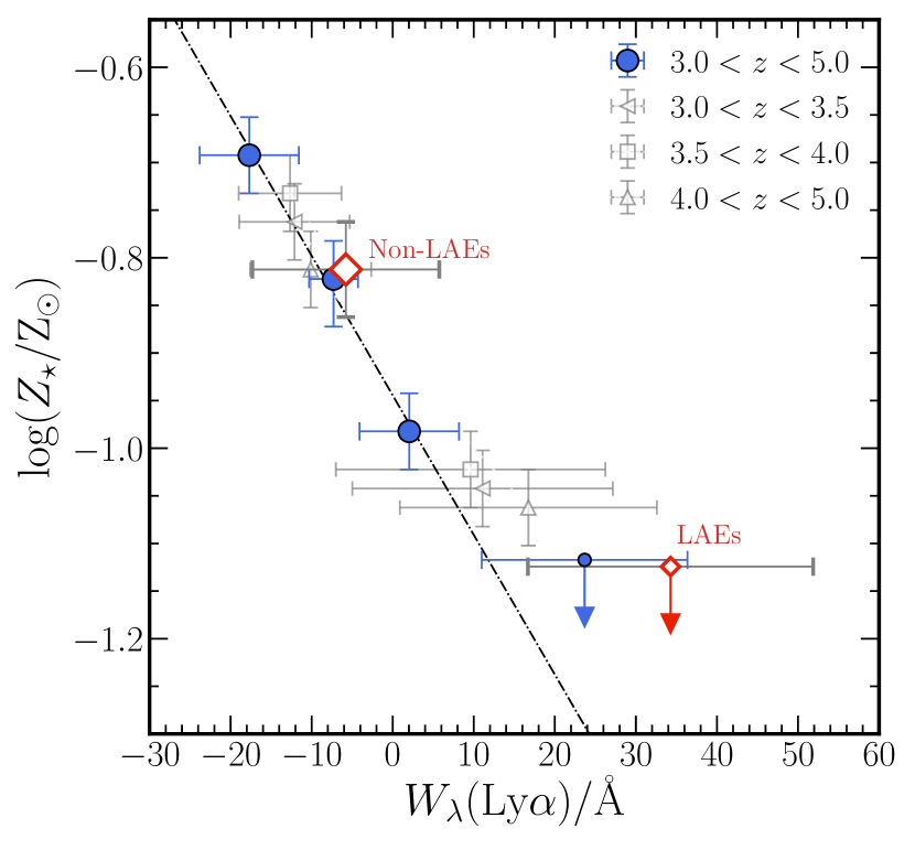
Figure 4: The relation between $W_{\lambda}$(Ly$\alpha$) and log($Z_{\ast}$/Z_⊙) for star-forming galaxies at $3\leq z\leq 5$. The blue circular data points with error bars show the data for the full sample split into quartiles of $W_{\lambda}$(Ly$\alpha$). The $W_{\lambda}$(Ly$\alpha$) values represent the median of all individual $W_{\lambda}$(Ly$\alpha$) values in each quartile. The $W_{\lambda}$(Ly$\alpha$) error bars represent the standard deviation of individual $W_{\lambda}$(Ly$\alpha$) values in each quartile (estimated as $\sigma\simeq 1.4826\times$ median absolute deviation). The red diamond data points show the sample split into LAEs ($W_{\lambda}$(Ly$\alpha$) $>20\rm{\AA}$) and non-LAEs ($W_{\lambda}$(Ly$\alpha$) $\leq 20\rm{\AA}$). Downward pointing arrows represent $68\%$ confidence upper limits on log($Z_{\ast}$/Z_⊙). The black dot-dashed line is a log-linear fit to the quartile data excluding the upper limit. The open grey data points show the sample split into three redshift bins as indicated in the figure legend (see text for details).

To assess the dependence of stellar metallicity ( $Z_{\star}$) on $W_{\lambda}$(Ly$\alpha$) we divided our sample into four independent quartiles of $W_{\lambda}$(Ly$\alpha$) and formed composite spectra following the method outlined in Cullen et al. (2019) (C19). Briefly, the individual contributing spectra were first shifted into the rest frame using the measured VANDELS redshift and then median-combined with an error spectrum estimated via bootstrap re-sampling. The composite spectra were sampled at $1\rm{\AA}/$pixel and covered the rest-frame wavelength range $1200-2000\rm{\AA}$ with an effective spectral resolution element of $3.0\rm{\AA}$. The median and standard deviation (determined from the MAD) of $W_{\lambda}$(Ly$\alpha$) for the four quartiles are given in Table 1. The composite spectra are shown in Fig. 3 where the transition from net Ly$\alpha$ emission to net Ly$\alpha$ absorption can clearly be seen.

Stellar metallicities for the $W_{\lambda}$(Ly$\alpha$) composites were determined following the method described in C19. Below we give a brief description of this method, but we refer interested readers to C19 for full details. We adopted the Starburst99 (SB99) high-resolution WM-Basic stellar population synthesis (SPS) models described in Leitherer et al. (2010), considering constant star-formation models over timescales of 100  Myr with $Z_{\ast}=(0.001,0.002,0.008,0.014,0.040)$. To fit the SB99 models to the composite spectra we used a Bayesian nested sampling algorithm implemented in the code multinest (Feroz & Hobson, 2008; Feroz et al., 2009). The four parameters in the fit were the stellar metallicity ( $Z_{\star}$) and three dust parameters based on a flexible and physically-motivated form of the attenuation curve described in Salim et al. (2018) (see also Noll et al., 2009). The prior in log($Z_{\ast}$/Z_⊙) was imposed by the SB99 models to be $-1.15<$ log($Z_{\ast}$/Z_⊙) $<1.45$. Since the models are provided for five fixed metallicity values, we linearly interpolated the logarithmic flux values between the models to generate a model at any metallicity within the prescribed range. The 1D posterior distribution for log($Z_{\ast}$/Z_⊙) was obtained by marginalizing over all other parameters in the fit. The best-fitting log($Z_{\ast}$/Z_⊙) value was then calculated from the $50$th percentile of this distribution along with the $68\%$ confidence limits. We note that the errors derived in this way represent the statistical errors for our fitting method and do not account for potential systematic effects related to our choice of SPS model and assumed star-formation history; for a discussion of these issues see C19. The best-fitting models for the four $W_{\lambda}$(Ly$\alpha$) stacks are shown in Fig. 3 and the best fitting log($Z_{\ast}$/Z_⊙) values with associated errors are given in Table 1.

Fig. 4 shows the resulting $W_{\lambda}$(Ly$\alpha$) $-$ log($Z_{\ast}$/Z_⊙) relation. The blue circular data points show the four $W_{\lambda}$(Ly$\alpha$) quartiles (Q1-Q4) from Fig. 3, with the downward pointing arrow representing the $68\%$ confidence upper limit on log($Z_{\ast}$/Z_⊙) for Q1. We observe a clear correlation between $W_{\lambda}$(Ly$\alpha$) and log($Z_{\ast}$/Z_⊙) of the form expected: galaxies that exhibit the strongest Ly$\alpha$ emission contain the lowest metallicity ionizing populations. Between the lowest and highest $W_{\lambda}$(Ly$\alpha$) quartiles the stellar metallicity decreases from  $Z_{\star}$/$Z_{\odot}$$=0.20\pm 0.02$ to  $Z_{\star}$/$Z_{\odot}$$\lesssim 0.07$ (i.e. greater than a factor 3 at $\simeq 6\sigma$ significance) and the log($Z_{\ast}$/Z_⊙) $-$ $W_{\lambda}$(Ly$\alpha$) relation (excluding the Q1 upper limit) can be approximately captured by a simple log-liner equation of the form:

$$\mathrm{log}(Z_{\ast}/\mathrm{Z}_{\odot})=-0.016(\pm 0.001)W_{\lambda}(\rm{Ly}\alpha)-0.95(\pm 0.01).$$ (1)

As a further check, we also produced composite spectra for the LAEs ($W_{\lambda}$(Ly$\alpha$) $>20\rm{\AA}$) and the non-LAEs ($W_{\lambda}$(Ly$\alpha$) $\leq 20\rm{\AA}$) in our sample. The red open diamonds in Fig. 4 show the average log($Z_{\ast}$/Z_⊙) and $W_{\lambda}$(Ly$\alpha$) for these populations, which are fully consistent with the quartile data. For our sample, the ionizing stellar population of non-LAE’s is $\gtrsim 2\times$ more metal enriched than for the LAE population. Again, however, we can only place an upper limit on log($Z_{\ast}$/Z_⊙) for the LAEs. In general, the fact that it is only possible to set an upper limit on  $Z_{\star}$ for the highest $W_{\lambda}$(Ly$\alpha$) galaxies highlights the fact that high-resolution stellar populations at  $Z_{\star}$/$Z_{\odot}$ $<<10\%$ will be required for modeling the low-mass, low-metallicity, galaxy population likely to have played a significant role in H i reionization at $z\gtrsim 6$.

We can rule out the possibility that the observed log($Z_{\ast}$/Z_⊙)$-$$W_{\lambda}$(Ly$\alpha$) relation is simply a product of differences in the median stellar mass of the $W_{\lambda}$(Ly$\alpha$) quartiles. This could potentially be an issue because of the known correlation between  $Z_{\star}$ and  $M_{\star}$ (i.e. the stellar MZR Gallazzi et al., 2005; Cullen et al., 2019). However we find, at least for quartiles Q2-Q4, that the stellar mass distributions have similar median values and variance (Table 1). The highest $W_{\lambda}$(Ly$\alpha$) quartile (Q1) has a slightly lower median  $M_{\star}$ value, although there is still significant overlap with Q2-Q4 given the large variance within each bin. Overall, there is no strong evidence to suggest that the change in  $Z_{\star}$ with $W_{\lambda}$(Ly$\alpha$) is being driven by differences in the stellar mass distributions of the composite spectra.

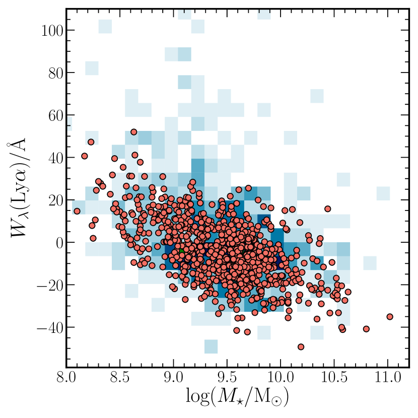
Figure 5: A comparison between the observed and simulated log($M_{\ast}$/M_⊙)$-$$W_{\lambda}$(Ly$\alpha$) relations. The underlying 2D histogram shows the observed distribution for the VANDELS sample (see also Fig. 1) and the orange circular points show a simulated distribution derived using the log($Z_{\ast}$/Z_⊙)$-$$W_{\lambda}$(Ly$\alpha$) relation (Fig. 4 and Equation 1) in combination with the stellar mass-metallicity relation from Cullen et al. (2019) (see text for details).

Finally, we checked for potential biases introduced by the relatively broad redshift distribution of our sample. A redshift bias could be a result of (i) a strong dependence of  $Z_{\star}$ on redshift, or (ii) the increasing IGM attenuation with redshift affecting the relative $W_{\lambda}$(Ly$\alpha$) values across our sample. As a basic test, we created six stacked spectra across three redshift bins, splitting each redshift bin into two bins of $W_{\lambda}$(Ly$\alpha$). As shown in Fig. 4, the $W_{\lambda}$(Ly$\alpha$)$-$ $Z_{\star}$ relation at each redshift is fully consistent with the relation across the full redshift range. This strongly suggests no systematic evolution of  $Z_{\star}$ within our sample, consistent with the results presented in Cullen et al. (2019). The effect of IGM absorption is more difficult to quantify however, since each galaxy will have its own unique sightline through the IGM. Nevertheless, it is expected that, on average, the galaxies at higher redshift will have a larger proportion of their Ly$\alpha$ flux blueward of $1216\rm{\AA}$ attenuated by neutral H i clouds along the line of sight (e.g. Pahl et al., 2020). This could potentially affect how the sample is binned by observed $W_{\lambda}$(Ly$\alpha$). As a simple test we corrected $W_{\lambda}$(Ly$\alpha$) of each galaxy using the relation between Ly$\alpha$ transmission and redshift reported in Songaila (2004). Splitting this IGM-corrected $W_{\lambda}$(Ly$\alpha$) distribution into quartiles has a very minor effect on the galaxies assigned to each quartile, and does not change the derived  $Z_{\star}$, although the median $W_{\lambda}$(Ly$\alpha$) values are clearly slightly larger. Unfortunately, it is not possible to determine the unique IGM correction for each galaxy, and in practice observed $W_{\lambda}$(Ly$\alpha$) is the only measurable quantity. Overall, we do not expect any strong redshift biases to be affecting the relation between observed $W_{\lambda}$(Ly$\alpha$) and  $Z_{\star}$.

3.2 Linking equivalent width, metallicity and mass

In C19 we presented the relation between log($Z_{\ast}$/Z_⊙) and log($M_{\ast}$/M_⊙) (i.e. the stellar MZR) for VANDELS star-forming galaxies at $2.5\leq z\leq 5.0$. It is interesting to test whether this relation and the log($Z_{\ast}$/Z_⊙)$-$$W_{\lambda}$(Ly$\alpha$) relation presented here are consistent with the observed distribution of log($M_{\ast}$/M_⊙) and $W_{\lambda}$(Ly$\alpha$) for the individual galaxies shown in Fig. 1. We note that, although the samples used here and in C19 are not fully independent, the three parameters of interest ( $Z_{\star}$,  $M_{\star}$, $W_{\lambda}$(Ly$\alpha$)) have been determined independently, and therefore consistency between the three resulting scaling relations would provide (i) evidence for the robustness of our parameter estimates and (ii) further insight into the nature of Ly$\alpha$ emission.

To test whether the three relations are self-consistent we performed a simple simulation. The C19 MZR, which can be approximated by an equation of the form

$$\mathrm{log}(Z_{\ast}/\mathrm{Z}_{\odot})=0.30(\pm 0.06)\mathrm{log}(M_{\ast}/\mathrm{M}_{\odot})+3.7(\pm 0.6),$$ (2)

was used to generate a value of log($Z_{\ast}$/Z_⊙) for each galaxy in our sample, with an additional scatter of $\sigma_{\rm{log}(Z_{\ast}/\rm{Z}_{\odot})}=0.1$ dex. Based on the log($Z_{\ast}$/Z_⊙) value, a value of $W_{\lambda}$(Ly$\alpha$) was generated using Equation 1, again adding a scatter of $\sigma_{W_{\lambda}(Ly\alpha)}=10\rm{\AA}$. The resulting distribution of simulated $W_{\lambda}$(Ly$\alpha$)$-$log($M_{\ast}$/M_⊙) data is shown overlaid on top of the observed distribution in Fig. 5. It can be seen that the bulk of observed $W_{\lambda}$(Ly$\alpha$) values are well-recovered, demonstrating an encouraging consistency between the three independently-measured quantities and highlighting the clear connection between the stellar mass of a galaxy, the metallicity of its young, ionizing, stellar population, and the emergent Ly$\alpha$ emission.

However, it is interesting to note that this simple model fails to account for the large $W_{\lambda}$(Ly$\alpha$) values ($\gtrsim 50\rm{\AA}$; $\simeq 5\%$ of the full sample) typically seen in galaxies with log($M_{\ast}$/M_⊙) $\lesssim 9.5$. At these values of $W_{\lambda}$(Ly$\alpha$), the MZR and log($Z_{\ast}$/Z_⊙)$-$$W_{\lambda}$(Ly$\alpha$) relations would predict significantly lower values of log($M_{\ast}$/M_⊙) than are observed. This failure of the model could be a result of a number of factors. Most obviously, the relations provided above are probably not applicable at the lowest stellar mass and $W_{\lambda}$(Ly$\alpha$) values in our sample, where at present we can only estimate upper limits on  $Z_{\star}$. Placing absolute constraints on  $Z_{\star}$ in this log($M_{\ast}$/M_⊙)/$W_{\lambda}$(Ly$\alpha$) regime will likely reveal that a more complex functional form is required to capture the true relations. Moreover, some of the physical assumptions used in our derivation of  $Z_{\star}$, which is based purely on analysing composite spectra, may not be applicable on a galaxy-by-galaxy basis. For example, the large $W_{\lambda}$(Ly$\alpha$) values seen in some low mass galaxies may be a result of recent bursts on star formation (e.g. Matthee et al., 2017) which elevate $W_{\lambda}$(Ly$\alpha$) with respect to the constant star formation histories assumed in our analysis. However, as this phenomenon only affects a small percentage of our full sample, we defer a more detailed analysis to a future work. Overall, it is clear that this simple model works remarkably well within the log($M_{\ast}$/M_⊙)/$W_{\lambda}$(Ly$\alpha$) range for which we can robustly determine  $Z_{\star}$.

Finally, it is interesting to note that the observed distribution can be recovered assuming relatively small values for the scatter in log($Z_{\ast}$/Z_⊙) and $W_{\lambda}$(Ly$\alpha$), implying a perhaps surprisingly small intrinsic scatter for these relations. Again, this is something we that we will be able to investigate in more detail in a future work utilizing the full VANDELS dataset.

3.3 The correlation with C iii] emission

Another prominent FUV emission feature, visible in Fig. 3, is the C iii]$\lambda\lambda 1907,1909$ emission line doublet. Theoretical models predict that the emergent C iii]$\lambda\lambda 1907,1909$ emission will increase towards lower  $Z_{\star}$ due to the increasing strength and hardness of the ionizing stellar continuum, which regulates both the gas temperature and ionization of $\rm{C}^{+}$ within H ii regions (Jaskot & Ravindranath, 2016; Senchyna et al., 2017; Schaerer et al., 2018; Nakajima et al., 2018). A variety of previous studies have reported a positive correlation between $W_{\lambda}$(Ly$\alpha$) and $W_{\lambda}$(C iii]) (e.g. Shapley et al., 2003; Stark et al., 2014; Rigby et al., 2015; Du et al., 2018; Le Fèvre et al., 2019) and it can clearly be seen from Fig. 3 that we observe a similar trend.

To quantify the relation, we measured $W_{\lambda}$(Ly$\alpha$) and $W_{\lambda}$(C iii]) directly from the composite spectra. $W_{\lambda}$(Ly$\alpha$) was measured using the same method as for the individual spectra, and the values with their 1$\sigma$ error bars are reported in Table 1. $W_{\lambda}$(C iii]) was measured by first subtracting a local continuum the in the region of the C iii] line and measuring the flux from the continuum-subtracted spectra; this flux was then divided by the average absolute continuum value in the wavelength range $1930-1950\rm{\AA}$. The final value of $W_{\lambda}$(C iii]) and its associated $1\sigma$ error bar was calculated using the same Monte Carlo approach adopted for the Ly$\alpha$ line measurements. Again, these values are reported in Table 1.

The results are shown in Fig. 6, where it can be seen that we find a clear positive correlation between $W_{\lambda}$(Ly$\alpha$) and $W_{\lambda}$(C iii]). This trend is consistent with the results of Shapley et al. (2003) and Du et al. (2018) at similar redshifts, with $W_{\lambda}$(C iii]) increasing by a factor 3 as $W_{\lambda}$(Ly$\alpha$) evolves from $\simeq-20\rm{\AA}$ to $20\rm{\AA}$. Moreover, as the equivalent width of both lines increase,  $Z_{\star}$ decreases. The trend we observe is therefore consistent with a scenario in which the hard ionizing SED of low metallicity stars is closely connected to the observed strength of both the Ly$\alpha$ and C iii] emission lines, which we discuss in more detail below. We also note that our composite spectra show no evidence for extreme $W_{\lambda}$(C iii]) values indicative of AGN photoionization ($\gtrsim 10\rm{\AA}$, Nakajima et al., 2018). Finally, it is worth noting that our results also imply that the strength of both Ly$\alpha$ and C iii] emission in galaxies should increase towards higher redshifts as the metallicity of stellar populations decreases further. Although the visibility of Ly$\alpha$ will be impeded by an increasing IGM H i fraction at $z>5$, the C iii] line should remain a promising line for study in the reionization era (e.g. Stark et al., 2014, 2017).

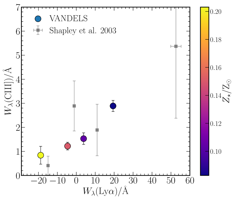
Figure 6: The relation between $W_{\lambda}$(Ly$\alpha$) and $W_{\lambda}$(C iii]). The circular data points with error bars show the results of our sample split into $W_{\lambda}$(Ly$\alpha$) quartiles colour-coded by the best-fitting stellar metallicity. In this case, the values of $W_{\lambda}$(Ly$\alpha$), $W_{\lambda}$(C iii]), and their respective errors are measured directly from the composite spectra as discussed in the text. The grey data points are values measured from composite spectra at similar redshifts from Shapley et al. (2003).

4 Discussion

The results presented above have demonstrated, for the first time, a direct correlation between $W_{\lambda}$(Ly$\alpha$) and  $Z_{\star}$ of the young O- and B-type stellar populations in high-redshift star-forming galaxies. In this section we briefly discuss this result with respect to other recent investigations of Ly$\alpha$ emission at high-redshift and finally consider the relative importance of intrinsic production/escape in governing the observed $W_{\lambda}$(Ly$\alpha$).

4.1 Factors governing the observed $W_{\lambda}$(Ly$\alpha$)

As discussed in Section 1, the observed $W_{\lambda}$(Ly$\alpha$) is dependent on both the production efficiency of Ly$\alpha$ photons within galactic H ii regions, and on the likelihood that these photons can escape the surrounding ISM/CGM. In this respect, a strong correlation between $W_{\lambda}$(Ly$\alpha$) and  $Z_{\star}$ is perhaps unsurprising. Stellar population synthesis models predict that the ionizing flux of a stellar population increases as stellar metallicity decreases (e.g. Schaerer, 2003; Stanway et al., 2016). An increase in the ionizing flux will naturally lead to an increase in the number of Ly$\alpha$ photons produced per unit star formation in lower metallicity galaxies. The increasing strength of the C iii]$\lambda\lambda 1907,1909$ emission line in tandem with Ly$\alpha$ also supports the idea that the harder ionizing continuum produced by low metallicity stellar populations is crucial in producing large $W_{\lambda}$(Ly$\alpha$). In addition, an increase in the ionizing photon flux may reduce the covering fraction or column density of neutral hydrogen, easing the escape of Ly$\alpha$ photons (e.g. Erb et al., 2014).

This picture is generally supported by previous studies that have correlated $W_{\lambda}$(Ly$\alpha$) with proxies of the ionizing flux and gas-phase metallicity. Most recently, Trainor et al. (2019) have shown that, as well as anti-correlating with the strength of low-ionization UV absorption lines, $W_{\lambda}$(Ly$\alpha$) correlates with the [O iii]/H $\beta$ and [O iii]/[O ii] nebular emission line ratios in star-forming galaxies at $2\lesssim z\lesssim 3$. Both of these ratios are known to be effective proxies for the ionization parameter as well as being potential signatures of low metallicity gas in galaxies (e.g. Nakajima & Ouchi, 2014; Cullen et al., 2016; Sanders et al., 2016; Strom et al., 2018). Similarly, Erb et al. (2016) have shown that Ly$\alpha$ emission is stronger in highly-ionized, low metallicity galaxies selected via their high [O iii]/H $\beta$ and low [N ii]/H $\alpha$ ratios. Comparable results have also been found using local ‘Green Pea’ galaxies (Yang et al., 2017). Generally, studies that probe gas-phase metallicity find that Ly$\alpha$ emission is enhanced in low metallicity environments (e.g. Finkelstein et al., 2011; Nakajima et al., 2013; Du et al., 2019). Our results add further support to this picture, by explicitly demonstrating that $W_{\lambda}$(Ly$\alpha$) increases in galaxies with lower stellar metallicity populations and, therefore, harder ionizing radiation fields.

Finally, another important factor in determining Ly$\alpha$ escape is the dust content of galaxies. Dust absorbs and scatters Ly$\alpha$ photons and therefore galaxies with higher dust covering fractions should have lower $W_{\lambda}$(Ly$\alpha$). Indeed, this correlation has been demonstrated in a number of different studies (e.g. Kornei et al., 2010; Pentericci et al., 2010; Marchi et al., 2019; Sobral & Matthee, 2019). Using the global shape of the composite spectra we can roughly estimate the typical FUV dust attenuation in our $W_{\lambda}$(Ly$\alpha$) quartiles. The FUV continuum slope of a galaxy, $\beta$, (where $f_{\lambda}\propto\lambda^{\beta}$) is known to be an effective proxy for the global dust attenuation at all redshifts, with bluer slopes indicating less dust (e.g. Meurer et al., 1999; Cullen et al., 2017). $\beta$ values were measured for each of the composite spectra following the method outlined in Cullen et al. (2017) and are given in Table 1. The slopes clearly become bluer (i.e. steeper) as $W_{\lambda}$(Ly$\alpha$) increases (as can also be clearly seen in Fig. 3). Converting these $\beta$ values into dust attenuation at $1500\rm{\AA}$ following the prescription of Cullen et al. (2017) indicates that $\rm{A}_{1500}$ decreases by a factor $\simeq 5$ between the highest and lowest $W_{\lambda}$(Ly$\alpha$) quartiles.

4.2 The relative importance of intrinsic production versus escape

Table 2: The ionizing continuum photon production rate ($N_{\rm{ion}}$) and resulting intrinsic $W_{\lambda}$(Ly$\alpha$) estimated from the best-fitting stellar population models in each $W_{\lambda}$(Ly$\alpha$) quartile. Values are calculated for the Starburst99 models used in this paper and also for the BPASSv2.2 models (Eldridge et al., 2017; Stanway & Eldridge, 2018) assuming the same star formation history and best-fitting stellar metallicity.

Starburst99
Qartile	log($Z_{\ast}$/Z⊙)	log($N_{\rm{ion}}/\rm{s}^{-1}$)	$W_{\lambda}$(Ly$\alpha$)${}_{\rm{int}}/\rm{\AA}$
Q1	$-0.69$	$53.28$	$102$
Q2	$-0.82$	$53.31$	$106$
Q3	$-0.98$	$52.32$	$107$
Q4	$<1.08$	$>52.32$	$>107$
BPASS v2.2
Q1	$-0.69$	$53.58$	$117$
Q2	$-0.82$	$53.60$	$121$
Q3	$-0.98$	$53.62$	$125$
Q4	$<1.08$	$>53.63$	$>127$

Figure 7: Intrinsic difference in Ly$\alpha$ equivalent width  ($\Delta$$W_{\lambda}$(Ly$\alpha$)_int) as a function of the observed difference ($\Delta$$W_{\lambda}$(Ly$\alpha$)_obs) between Q_N and Q4. For the blue circular data points, $\Delta$$W_{\lambda}$(Ly$\alpha$)_int was calculated based on the ionizing continuum properties of the best-fitting Starburst99 model (see text for details). For the red square data points, $\Delta$$W_{\lambda}$(Ly$\alpha$)_int was calculated using the BPASSv2.2 models assuming the same star formation history and best-fitting stellar metallicity. If the data fell on the 1:1 relation (dashed black line) this would imply that changes in the ionizing production efficiency of the stellar population with  $Z_{\star}$ alone could account for the observed variation in $W_{\lambda}$(Ly$\alpha$).

While it is clear that our results are consistent with a picture in which the observed $W_{\lambda}$(Ly$\alpha$) depends both upon the intrinsic production rate of Ly$\alpha$ photons and on the overall Ly$\alpha$ opacity (or equivalently the Ly$\alpha$ escape fraction), we can also attempt to estimate the relative importance of these two physical effects. For each $W_{\lambda}$(Ly$\alpha$) quartile we first determined the rate of ionizing photon emission ($N_{\rm{ion}}$ [s^-1]) from the best-fitting Starburst99 model by integrating the spectrum below $912\rm{\AA}$. Then, assuming a simple conversion between $N_{\rm{ion}}$ and H $\alpha$ luminosity (Kennicutt, 1998) and an intrinsic Ly$\alpha$/H $\alpha$ ratio of 8.7 (Osterbrock, 1989), we estimated the Ly$\alpha$ luminosity as

$$L(\mathrm{Ly}\alpha)[\mathrm{erg}\mathrm{s}^{-1}]=1.18\times 10^{-11}N_{\rm{ion}}[\mathrm{s}^{-1}].$$ (3)

The continuum luminosity density ($L_{\lambda,\rm{UV}}$) was defined as the median model luminosity density between $1228-1255\rm{\AA}$ and the intrinsic equivalent width ($W_{\lambda}$(Ly$\alpha$)_int) estimated as $L(\mathrm{Ly}\alpha)/L_{\lambda,\rm{UV}}$. Values for $N_{\rm{ion}}$ and $W_{\lambda}$(Ly$\alpha$)_int are given in Table 2. We also report, in Table 2, the same values calculated using the BPASSv2.2 SPS models (Eldridge et al., 2017; Stanway & Eldridge, 2018), where we have assumed the same star formation history and best-fitting metallicity as for the Starburst99 models. We note that for Q1, since we can only estimate and upper limit on  $Z_{\star}$, we can also only estimate a lower limit on $W_{\lambda}$(Ly$\alpha$)_int. We also note that this analysis assumes a $0\%$ escape fraction of ionizing continuum photons ($f_{\rm{esc}}=0$). However, given the low average escape fraction of galaxies at these redshifts (e.g. $f_{\rm{esc}}=0.09\pm 0.01$, Steidel et al., 2018), for the purpose of this discussion it should be a reasonable assumption.

It can clearly be seen that the values of $W_{\lambda}$(Ly$\alpha$)_int reported in Table 2 are much larger than the observed $W_{\lambda}$(Ly$\alpha$) values in Table 1, which is unsurprising given the relatively large Ly$\alpha$ opacities expected in general. Perhaps more interesting is the fact that the differences in $W_{\lambda}$(Ly$\alpha$)_int across the quartiles $-$ which are due exclusively to changes in the ionizing continuum strength with  $Z_{\star}$ $-$ are much smaller than the observed differences in $W_{\lambda}$(Ly$\alpha$). This is clearly illustrated in Fig. 7. For the Starburst99 models, we estimate that $W_{\lambda}$(Ly$\alpha$)_int varies by $\simeq 5\rm{A}$ between Q4 and Q1, which accounts for only $\simeq 12\%$ of the total observed variation ($\simeq 40\rm{\AA}$). The value is slightly larger assuming the BPASSv2.2 models ($\simeq 10\rm{A}$) but is still a minority effect ($\simeq 25\%$).

This result suggests that, on average, the change in $W_{\lambda}$(Ly$\alpha$) across the quartiles is being driven primarily by a variation in the Ly$\alpha$ escape fraction in low  $Z_{\star}$ galaxies ($\simeq 75-85\%$ contribution) as opposed to the intrinsic production rate of Ly$\alpha$ photons ($\simeq 15-25\%$ contribution). Based on this picture, the strong correlation between $W_{\lambda}$(Ly$\alpha$) and  $Z_{\star}$ we observe, which results in low  $Z_{\star}$ galaxies exhibiting stronger Ly$\alpha$ emission, is a result of three factors: (i) an increase in the production rate of Ly$\alpha$ photons at lower  $Z_{\star}$, (ii) a decrease in the covering fraction of H i gas due to stronger ionizing continua at lower  $Z_{\star}$ and, (iii) a decrease in the overall dust content of galaxies at lower  $Z_{\star}$, with the combination of (ii) and (iii) providing the dominant contribution to the observed relation. Finally, we stress that these conclusions apply to the star-forming population on average, and assume that 100 Myr constant star formation histories are a reasonable approximation for the majority of the FUV spectra at these redshifts (Steidel et al., 2016; Cullen et al., 2019). For individual galaxies with bursty star-formation histories and UV-ages $\lesssim 20$ Myr (e.g. galaxies with the largest $W_{\lambda}$(Ly$\alpha$); Fig 5) there may also be age-dependent affects governing the relative $N_{\rm{ion}}$ (e.g. Stanway et al., 2016).

5 Conclusions

In this paper we have presented, for the first time, an investigation into the correlation between Ly$\alpha$ equivalent width and stellar metallicity for a sample of 768 star-forming galaxies at $3\leq z\leq 5$ drawn from the VANDELS survey (McLure et al., 2018; Pentericci et al., 2018). Our main results can be summarised as follows:

1. Splitting our sample into four $W_{\lambda}$(Ly$\alpha$) quartiles we observe a strong anti-correlation between $W_{\lambda}$(Ly$\alpha$) and  $Z_{\star}$. We find that  $Z_{\star}$ decreases by a factor $\gtrsim 3$ between the lowest $W_{\lambda}$(Ly$\alpha$) quartile ($\langle$$W_{\lambda}$(Ly$\alpha$)$\rangle=-18\rm{\AA}$) and the highest $W_{\lambda}$(Ly$\alpha$) quartile ($\langle$$W_{\lambda}$(Ly$\alpha$)$\rangle=24\rm{\AA}$).

2. The same relation is observed if we split our sample into LAEs ($W_{\lambda}$(Ly$\alpha$) $>20\rm{\AA}$) and non-LAEs ($W_{\lambda}$(Ly$\alpha$) $\leq 20\rm{\AA}$). On average, the non-LAEs in our sample are $\gtrsim 2\times$ more metal enriched than the LAE population.

3. Employing a simple simulation, we show that the $W_{\lambda}$(Ly$\alpha$)-log($Z_{\ast}$/Z_⊙) relation presented here, in combination with the stellar MZR presented in Cullen et al. (2019), can reproduce the observed $W_{\lambda}$(Ly$\alpha$)-log($M_{\ast}$/M_⊙) distribution for $\simeq 95\%$ of our sample. Crucially, however, this simple model fails to account for the $\simeq 5\%$ of our sample with $W_{\lambda}$(Ly$\alpha$) $\gtrsim 50\rm{\AA}$ (and typically with log($M_{\ast}$/M_⊙) $\lesssim 9.5$). This result could indicate that our assumption of a constant star-formation history breaks down for some individual galaxies at the lowest stellar masses, where bursty star-formation histories may become more prevalent.

4. We observe a clear correlation between $W_{\lambda}$(Ly$\alpha$) and $W_{\lambda}$(C iii]) consistent with previous measurements at similar redshifts. Our results indicate that the strength of both lines increases with decreasing stellar metallicity. This provides further evidence to support the idea that the harder ionizing continuum spectra emitted by low metallicity stellar populations plays a role in modulating both the emergent Ly$\alpha$ and C iii] emission in star-forming galaxies.

5. Finally, by estimating the intrinsic Ly$\alpha$ equivalent widths ($W_{\lambda}$(Ly$\alpha$)_int) for each quartile, we show that the contribution to the observed variation of $W_{\lambda}$(Ly$\alpha$) due to changes in the ionizing spectrum with  $Z_{\star}$ is of the order $\simeq 15-25\%$. The dominant contribution ($75-85\%$) is therefore a variation in the Ly$\alpha$ opacity (or escape fraction) with  $Z_{\star}$, presumably due to a combination of lower H i and dust covering fractions in low  $Z_{\star}$ galaxies.

Overall, the results presented here provide further evidence$-$using, for the first time, direct estimates of  $Z_{\star}$$-$ for a scenario in which low-mass, less dust obscured, galaxies with low-metallicity ionizing stellar populations are both the most efficient producers of Ly$\alpha$ photons, and the systems from which those photons have the highest likelihood of escape.

6 Acknowledgments

FC, RJM, JSD, AC and DJM acknowledge the support of the UK Science and Technology Facilities Council. A. Cimatti acknowledges the grants ASI n.2018-23-HH.0, PRIN MIUR 2015 and PRIN MIUR 2017 - 20173ML3WW 001. This work is based on data products from observations made with ESO Telescopes at La Silla Paranal Observatory under ESO programme ID 194.A-2003(E-Q). We thank the referee for useful suggestions that have improved this paper. This research made use of Astropy, a community-developed core Python package for Astronomy (Astropy Collaboration et al., 2018), NumPy and SciPy (Oliphant, 2007), Matplotlib (Hunter, 2007), IPython (Pérez & Granger, 2007) and NASA’s Astrophysics Data System Bibliographic Services.

¹SUPAScottish Universities Physics Alliance, Institute for Astronomy, University of Edinburgh, Royal Observatory, Edinburgh EH9 3HJ
²Department of Physics and Astronomy, University of California, Los Angeles, 430 Portola Plaza, Los Angeles, CA 90095, USA
³Instituto de Investigación Multidisciplinar en Ciencia y Tecnología, Universidad de La Serena, Raúl Bitrán 1305, La Serena, Chile
⁴Departamento de Física y Astronomía, Universidad de La Serena, Av. Juan Cisternas 1200 Norte, La Serena, Chile
⁵INAF - Osservatorio Astronomico di Bologna, via P. Gobetti 93/3,I-40129, Bologna, Italy
⁶INAF$-$Osservatorio Astronomico di Roma, Via Frascati 33, I-00040 Monte Porzio Catone (RM), Italy
⁷University of Bologna, Department of Physics and Astronomy (DIFA) Via Gobetti 93/2- 40129, Bologna, Italy
⁸INAF - Osservatorio Astrofisico di Arcetri, Largo E. Fermi 5, I-50125, Firenze, Italy
⁹European Southern Observatory, Karl-Schwarzschild-Str. 2, 86748 Garching b. München, Germany
¹⁰INAF-Astronomical Observatory of Trieste, via G.B. Tiepolo 11, 34143 Trieste, Italy
¹¹INAF-IASF Milano, via Bassini 15, I-20133, Milano, Italy
¹²Núcleo de Astronomía, Facultad de Ingeniería, Universidad Diego Portales, Av. Ejército 441, Santiago, Chile
¹³Department of Physics, University of Oxford, Keble Road, Oxford OX1 3RH, UK
¹⁴Department of Physics and Astronomy, University of the Western Cape, Private Bag X17, Bellville, Cape Town, 7535, South Africa
¹⁵The Cosmic Dawn Center, Niels Bohr Institute, University of Copenhagen, Juliane Maries Vej 30, DK-2100 Copenhagen Ø, Denmark
¹⁶Space Telescope Science Institute, 3700 San Martin Drive, Baltimore, MD 21218, USA
¹⁷Astronomy Department, University of Massachusetts, Amherst, MA 01003, USA

References

- Asplund et al. (2009) Asplund M., Grevesse N., Sauval A. J., Scott P., 2009, Annual Review of Astronomy and Astrophysics, 47, 481
- Astropy Collaboration et al. (2018) Astropy Collaboration et al., 2018, AJ, 156, 123
- Bruzual & Charlot (2003) Bruzual G., Charlot S., 2003, MNRAS, 344, 1000
- Buchner et al. (2014) Buchner J., et al., 2014, A&A, 564, A125
- Calzetti et al. (2000) Calzetti D., Armus L., Bohlin R. C., Kinney A. L., Koornneef J., Storchi-Bergmann T., 2000, ApJ, 533, 682
- Cassata et al. (2015) Cassata P., et al., 2015, A&A, 573, A24
- Castellano et al. (2014) Castellano M., et al., 2014, A&A, 566, A19
- Chabrier (2003) Chabrier G., 2003, PASP, 115, 763
- Charlot & Fall (1993) Charlot S., Fall S. M., 1993, ApJ, 415, 580
- Cullen et al. (2014) Cullen F., Cirasuolo M., McLure R. J., Dunlop J. S., Bowler R. A. A., 2014, MNRAS, 440, 2300
- Cullen et al. (2016) Cullen F., Cirasuolo M., Kewley L. J., McLure R. J., Dunlop J. S., Bowler R. A. A., 2016, MNRAS, 460, 3002
- Cullen et al. (2017) Cullen F., McLure R. J., Khochfar S., Dunlop J. S., Dalla Vecchia C., 2017, MNRAS, 470, 3006
- Cullen et al. (2019) Cullen F., et al., 2019, MNRAS, 487, 2038
- Dijkstra (2014) Dijkstra M., 2014, Publ. Astron. Soc. Australia, 31, e040
- Du et al. (2018) Du X., et al., 2018, ApJ, 860, 75
- Du et al. (2019) Du X., Shapley A. E., Tang M., Stark D. P., Martin C. L., Mobasher B., Topping M. W., Chevallard J., 2019, arXiv e-prints, p. arXiv:1910.11877
- Eldridge et al. (2017) Eldridge J. J., Stanway E. R., Xiao L., McClelland L. A. S., Taylor G., Ng M., Greis S. M. L., Bray J. C., 2017, Publ. Astron. Soc. Australia, 34, e058
- Erb et al. (2010) Erb D. K., Pettini M., Shapley A. E., Steidel C. C., Law D. R., Reddy N. A., 2010, ApJ, 719, 1168
- Erb et al. (2014) Erb D. K., et al., 2014, ApJ, 795, 33
- Erb et al. (2016) Erb D. K., Pettini M., Steidel C. C., Strom A. L., Rudie G. C., Trainor R. F., Shapley A. E., Reddy N. A., 2016, ApJ, 830, 52
- Feroz & Hobson (2008) Feroz F., Hobson M. P., 2008, MNRAS, 384, 449
- Feroz et al. (2009) Feroz F., Hobson M. P., Bridges M., 2009, MNRAS, 398, 1601
- Finkelstein et al. (2011) Finkelstein S. L., et al., 2011, ApJ, 729, 140
- Fontanot et al. (2014) Fontanot F., Cristiani S., Pfrommer C., Cupani G., Vanzella E., 2014, MNRAS, 438, 2097
- Gallazzi et al. (2005) Gallazzi A., Charlot S., Brinchmann J., White S. D. M., Tremonti C. A., 2005, MNRAS, 362, 41
- Grogin et al. (2011) Grogin N. A., et al., 2011, ApJS, 197, 35
- Hathi et al. (2016) Hathi N. P., et al., 2016, A&A, 588, A26
- Hayes et al. (2014) Hayes M., et al., 2014, ApJ, 782, 6
- Heckman et al. (2011) Heckman T. M., et al., 2011, ApJ, 730, 5
- Hunter (2007) Hunter J. D., 2007, Computing In Science & Engineering, 9, 90
- Jaskot & Ravindranath (2016) Jaskot A. E., Ravindranath S., 2016, ApJ, 833, 136
- Kennicutt (1998) Kennicutt Robert C. J., 1998, ARA&A, 36, 189
- Kewley et al. (2013) Kewley L. J., Dopita M. A., Leitherer C., Davé R., Yuan T., Allen M., Groves B., Sutherland R., 2013, ApJ, 774, 100
- Kewley et al. (2019) Kewley L. J., Nicholls D. C., Sutherland R. S., 2019, ARA&A, 57, 511
- Koekemoer et al. (2011) Koekemoer A. M., et al., 2011, ApJS, 197, 36
- Kornei et al. (2010) Kornei K. A., Shapley A. E., Erb D. K., Steidel C. C., Reddy N. A., Pettini M., Bogosavljević M., 2010, ApJ, 711, 693
- Kriek et al. (2009) Kriek M., van Dokkum P. G., Labbé I., Franx M., Illingworth G. D., Marchesini D., Quadri R. F., 2009, ApJ, 700, 221
- Law et al. (2012) Law D. R., Steidel C. C., Shapley A. E., Nagy S. R., Reddy N. A., Erb D. K., 2012, ApJ, 759, 29
- Le Fèvre et al. (2019) Le Fèvre O., et al., 2019, A&A, 625, A51
- Leitherer et al. (2010) Leitherer C., Ortiz Otálvaro P. A., Bresolin F., Kudritzki R.-P., Lo Faro B., Pauldrach A. W. A., Pettini M., Rix S. A., 2010, ApJS, 189, 309
- Marchi et al. (2018) Marchi F., et al., 2018, A&A, 614, A11
- Marchi et al. (2019) Marchi F., et al., 2019, A&A, 631, A19
- Matthee et al. (2017) Matthee J., Sobral D., Darvish B., Santos S., Mobasher B., Paulino-Afonso A., Röttgering H., Alegre L., 2017, MNRAS, 472, 772
- McLure et al. (2018) McLure R. J., et al., 2018, MNRAS, 479, 25
- Meurer et al. (1999) Meurer G. R., Heckman T. M., Calzetti D., 1999, ApJ, 521, 64
- Nakajima & Ouchi (2014) Nakajima K., Ouchi M., 2014, MNRAS, 442, 900
- Nakajima et al. (2013) Nakajima K., Ouchi M., Shimasaku K., Hashimoto T., Ono Y., Lee J. C., 2013, ApJ, 769, 3
- Nakajima et al. (2018) Nakajima K., et al., 2018, A&A, 612, A94
- Nestor et al. (2013) Nestor D. B., Shapley A. E., Kornei K. A., Steidel C. C., Siana B., 2013, ApJ, 765, 47
- Noll et al. (2009) Noll S., Burgarella D., Giovannoli E., Buat V., Marcillac D., Muñoz-Mateos J. C., 2009, A&A, 507, 1793
- Oliphant (2007) Oliphant T. E., 2007, Computing in Science & Engineering, 9, 10
- Osterbrock (1989) Osterbrock D. E., 1989, Astrophysics of gaseous nebulae and active galactic nuclei
- Oyarzún et al. (2016) Oyarzún G. A., et al., 2016, ApJ, 821, L14
- Oyarzún et al. (2017) Oyarzún G. A., Blanc G. A., González V., Mateo M., Bailey John I. I., 2017, ApJ, 843, 133
- Pahl et al. (2020) Pahl A. J., Shapley A., Faisst A. L., Capak P. L., Du X., Reddy N. A., Laursen P., Topping M. W., 2020, MNRAS,
- Pentericci et al. (2010) Pentericci L., Grazian A., Scarlata C., Fontana A., Castellano M., Giallongo E., Vanzella E., 2010, A&A, 514, A64
- Pentericci et al. (2018) Pentericci L., et al., 2018, A&A, 616, A174
- Pérez & Granger (2007) Pérez F., Granger B. E., 2007, Computing in Science & Engineering, 9, 21
- Rigby et al. (2015) Rigby J. R., Bayliss M. B., Gladders M. D., Sharon K., Wuyts E., Dahle H., Johnson T., Peña-Guerrero M., 2015, ApJ, 814, L6
- Robertson et al. (2015) Robertson B. E., Ellis R. S., Furlanetto S. R., Dunlop J. S., 2015, ApJ, 802, L19
- Rogers et al. (2014) Rogers A. B., et al., 2014, MNRAS, 440, 3714
- Salim et al. (2018) Salim S., Boquien M., Lee J. C., 2018, ApJ, 859, 11
- Sanders et al. (2016) Sanders R. L., et al., 2016, ApJ, 816, 23
- Schaerer (2003) Schaerer D., 2003, A&A, 397, 527
- Schaerer et al. (2018) Schaerer D., Izotov Y. I., Nakajima K., Worseck G., Chisholm J., Verhamme A., Thuan T. X., de Barros S., 2018, A&A, 616, L14
- Schreiber et al. (2018) Schreiber C., et al., 2018, A&A, 611, A22
- Senchyna et al. (2017) Senchyna P., et al., 2017, MNRAS, 472, 2608
- Shapley et al. (2003) Shapley A. E., Steidel C. C., Pettini M., Adelberger K. L., 2003, ApJ, 588, 65
- Sobral & Matthee (2019) Sobral D., Matthee J., 2019, A&A, 623, A157
- Song et al. (2014) Song M., et al., 2014, ApJ, 791, 3
- Songaila (2004) Songaila A., 2004, AJ, 127, 2598
- Stanway & Eldridge (2018) Stanway E. R., Eldridge J. J., 2018, MNRAS, 479, 75
- Stanway et al. (2016) Stanway E. R., Eldridge J. J., Becker G. D., 2016, MNRAS, 456, 485
- Stark et al. (2014) Stark D. P., et al., 2014, MNRAS, 445, 3200
- Stark et al. (2017) Stark D. P., et al., 2017, MNRAS, 464, 469
- Steidel et al. (2014) Steidel C. C., et al., 2014, ApJ, 795, 165
- Steidel et al. (2016) Steidel C. C., Strom A. L., Pettini M., Rudie G. C., Reddy N. A., Trainor R. F., 2016, ApJ, 826, 159
- Steidel et al. (2018) Steidel C. C., Bogosavljević M., Shapley A. E., Reddy N. A., Rudie G. C., Pettini M., Trainor R. F., Strom A. L., 2018, ApJ, 869, 123
- Strom et al. (2018) Strom A. L., Steidel C. C., Rudie G. C., Trainor R. F., Pettini M., 2018, ApJ, 868, 117
- Trainor et al. (2015) Trainor R. F., Steidel C. C., Strom A. L., Rudie G. C., 2015, ApJ, 809, 89
- Trainor et al. (2016) Trainor R. F., Strom A. L., Steidel C. C., Rudie G. C., 2016, ApJ, 832, 171
- Trainor et al. (2019) Trainor R. F., Strom A. L., Steidel C. C., Rudie G. C., Chen Y., Theios R. L., 2019, ApJ, 887, 85
- Verhamme et al. (2017) Verhamme A., Orlitová I., Schaerer D., Izotov Y., Worseck G., Thuan T. X., Guseva N., 2017, A&A, 597, A13
- Yang et al. (2017) Yang H., et al., 2017, ApJ, 844, 171