Precise determination of $\alpha_{s}$ from relativistic quarkonium sum rules

Abstract

We determine the strong coupling $\alpha_{s}(m_{Z})$ from dimensionless ratios of roots of moments of the charm- and bottom-quark vector and charm pseudo-scalar correlators, dubbed $R_{q}^{X,n}\equiv(M_{q}^{X,n})^{\frac{1}{n}}/(M_{q}^{X,n+1})^{\frac{1}{n+1}}$, with $X=V,P$, as well as from the $0$-th moment of the charm pseudo-scalar correlator, $M_{c}^{P,0}$. In the quantities we use, the mass dependence is very weak, entering only logarithmically, starting at $\mathcal{O}(\alpha_{s}^{2})$. We carefully study all sources of uncertainties, paying special attention to truncation errors, and making sure that order-by-order convergence is maintained by our choice of renormalization scale variation. In the computation of the experimental uncertainty for the moment ratios, the correlations among individual moments are properly taken into account. Additionally, in the perturbative contributions to experimental vector-current moments, $\alpha_{s}(m_{Z})$ is kept as a free parameter such that our extraction of the strong coupling is unbiased and based only on experimental data. The most precise extraction of $\alpha_{s}$ from vector correlators comes from the ratio of the charm-quark moments $R_{c}^{V,2}$ and reads $\alpha_{s}(m_{Z})=0.1168\pm 0.0019$, as we have recently discussed in a companion letter. From bottom moments, using the ratio $R_{b}^{V,2}$, we find $\alpha_{s}(m_{Z})=0.1186\pm 0.0048$. Our results from the lattice pseudo-scalar charm correlator agree with the central values of previous determinations, but have larger uncertainties due to our more conservative study of the perturbative error. Averaging the results obtained from various lattice inputs for the $n=0$ moment we find $\alpha_{s}(m_{Z})=0.1177\pm 0.0020$. Combining experimental and lattice information on charm correlators into a single fit we obtain $\alpha_{s}(m_{Z})=0.1170\pm 0.0014$, which is the main result of this article.

1 Introduction

The strong coupling $\alpha_{s}$ is the central quantity governing quantum chromodynamics (QCD). It is a key parameter to all observables computed in perturbation theory relevant for facilities such as the LHC or future $e^{+}e^{-}$ colliders, which have an extensive program for determining top-quark and Higgs-boson properties such as their masses and couplings. It also plays a central role in flavor physics and in the determination of the masses of charmonium and bottomonium bound states. This parameter is also crucial for searches of physics beyond the Standard Model since it largely determines the size of the associated background. For a review on recent progress see e.g. Refs. Pich:2018lmu ; Salam:2017qdl .

A powerful method to determine parameters related to the strong interactions such as quark masses and $\alpha_{s}$ are QCD sum rules based on weighted integrals of the total hadronic cross section $R_{q\bar{q}}$ (with $q=c,b$)

$$R_{q\bar{q}}(s)=\frac{3s}{4\pi\alpha^{2}}\sigma_{e^{+}e^{-}\to\,q\bar{q}\,+X}(s)\simeq\dfrac{\sigma_{e^{+}e^{-}\to\,q\bar{q}\,+X}(s)}{\sigma_{e^{+}e^{-}\to\,\mu^{+}\mu^{-}}(s)}\,.$$ (1)

Particularly important for our work are the inverse moments, $M_{q}^{V,n}$, of $R_{q\bar{q}}(s)$ defined as

$$M_{q}^{V,n}=\int\!\dfrac{{\rm d}s}{s^{n+1}}R_{q\bar{q}}(s)\,.\qquad\quad$$ (2)

Using analyticity and unitarity, these can be related to the coefficients of the Taylor expansion of the quark vector-current correlator around $s=0$, which can be computed rigorously in perturbative QCD (pQCD) for $n$ not too large.

A shortcoming of using moments $M_{q}^{V,n}$ is that, while the integration in Eq. (2) over the normalized cross section extends all the way to infinity, experimental data are limited to a finite energy range. If the energy of the last measured cross section is sufficiently large, one can safely use the theoretical prediction for the $R$-ratio in perturbation theory as a substitute (the region is sometimes referred to as the continuum), applying some penalty to reduce the model dependence. For the charm cross section the data above threshold spans a wide range of energies such that even for $n=1$ the computed moment is fairly insensitive to how the continuum is treated Dehnadi:2011gc . On the other hand, bottom moments with low values of $n$ do depend strongly on the continuum such that $M_{b}^{V,1}$ cannot be used for any competitive determination of the bottom-quark mass Corcella:2002uu ; Dehnadi:2015fra — a situation that could change if data at larger energies became available. Here, since we are interested in a precise extraction of $\alpha_{s}$, the continuum contribution must be treated carefully, in a way that avoids any possible contamination of the extracted values.

Theoretically, the moments $M_{q}^{X,n}$ are governed by the typical scale $m_{q}/n\gtrsim\Lambda_{\rm QCD}$. This is easy to understand since large values of $n$ have more weight in the narrow resonances such that a non-relativistic treatment becomes necessary. For small values of $n$ one can compute the moments in perturbative QCD supplemented by non-perturbative power corrections parametrized in terms of local condensates. This framework is known as the operator product expansion (OPE) Shifman:1978bx ; Shifman:1978by . It turns out that the perturbative term overly dominates the series (even more so for the bottom quark) and the leading (gluon) condensate is introduced mainly as an estimate of the size of non-perturbative corrections. This method goes under the name of relativistic quarkonium sum rules.

An interesting alternative which does not suffer from problems related to the continuum are moments of the pseudo-scalar quark-current correlator, which can be accurately computed in lattice QCD Allison:2008xk — although, so far, precise simulations exist only for the charm quark. Interestingly, the $0$-th moment of this correlator is physical, and quite insensitive to the charm-quark mass, which makes it an ideal candidate to determine $\alpha_{s}$. On the other hand, it has been shown that the perturbative series of the pseudo-scalar moments (at least for $n>0$) displays a quite poor convergence Dehnadi:2015fra .

A lot of progress has been made in the lattice community for determining QCD parameters from the pseudo-scalar correlator since the pioneering work of Ref. Allison:2008xk , in which the charm-quark mass and the strong coupling were extracted (the former with high accuracy). Focusing on $\alpha_{s}$, the follow-up paper by HPQCD McNeile:2010ji already claimed half-percent accuracy at the $Z$-boson mass with a value very close to the world average, while Refs. Maezawa:2016vgv and Petreczky:2019ozv have somewhat smaller central values and slightly larger uncertainties ($0.7\,\%$ and $1\%$, respectively). The latter references introduced an interesting alternative strategy to determine $\alpha_{s}$: the use of ratios of moments for which the mass dependence largely cancels; a strategy that we extend and exploit here also for the vector-current moments.

So far, nearly all lattice analyses with sub-percent accuracy on $\alpha_{s}(m_{Z})$ estimate the perturbative uncertainties in essentially the same way: fixing the renormalization scale to some default value and adding an estimate for the first unknown perturbative coefficient. The truncation error is estimated by either varying the size of the guessed term or comparing the values of the strong-coupling constant obtained including or not the next term (an exception to this paradigm is the analysis of Ref. Nakayama:2016atf ). However, as argued in Refs. Dehnadi:2011gc ; Dehnadi:2015fra , the renormalization scale of $\overline{m}_{q}$ plays an important role in realistic estimates of perturbative uncertainties. In Ref. Nakayama:2016atf , which only uses ratios of moments, perturbative uncertainties are estimated performing renormalization scale variation in a manner analogous to Refs. Dehnadi:2011gc ; Dehnadi:2015fra . In particular, renormalization scales for $\alpha_{s}$ and the heavy-quark mass are floated independently within a certain range. Their result is compatible with the world average, but the quoted uncertainties are more conservative, achieving only $2.2\%$ accuracy. This shows that, while it can probably be argued that the computation of the moments on the lattice is fairly under control, one could question some of the estimates of theory incertitudes found in the literature.

In this article we extract the strong coupling with $n_{f}=4$ and $n_{f}=5$ from QCD sum rules analyzing dimensionless mass-insensitive ratios of the moments $M_{q}^{V,n}$ and $M_{q}^{P,n}$, denoted $R_{q}^{X,n}$ and defined in Eq. (8). This type of strategy was originally introduced for pseudo-scalar moments computed on the lattice Maezawa:2016vgv ; Petreczky:2019ozv and, to the best of our knowledge, was applied to vector-current correlators, whose moments can be obtained using real experimental data on $R_{q\bar{q}}(s)$, for the first time in a companion paper Boito:2019pqp . Here, we provide further details on the analysis of Ref. Boito:2019pqp , extend the method to bottom vector-current moments, and, finally, apply the same strategy to the lattice-determined pseudo-scalar moment ratios of the charm current.

On the experimental side, we compute the ratios $R_{q}^{V,n}$ using data on narrow resonances and the total hadronic cross section above the charm and bottom open thresholds, supplemented with perturbation theory in the regions where no measurements exist (and to subtract the $uds$ background from charmonium data). Since our goal is to perform a rigorous extraction of $\alpha_{s}$, the value of the coupling used as input in the perturbative expressions must be kept as a free parameter, such that $\alpha_{s}$ is extracted from the experimental data without any bias. On the theoretical side, we carefully examine perturbative uncertainties and conclude that the renormalization scales of $\alpha_{s}$ and the $\overline{\mathrm{MS}}$ quark mass have to be varied independently within a certain range to avoid theoretical biases. Using this approach, we also perform a reanalysis of lattice data on the ratios of moments $R_{c}^{P,n}$ and the $M_{c}^{P,0}$ regular moment for the pseudo-scalar charm correlator. The method provides a reliable extraction of $\alpha_{s}$ and, in particular for the vector-current charm-quark ratios, $R_{c}^{V,n}$, the values obtained for $\alpha_{s}^{(n_{f}=5)}(m_{Z})$ are competitive given the accuracy of current experimental data. Finally, results from lattice QCD and the charm vector moment ratios can be unambiguously combined to obtain an even more precise strong coupling determination.

This paper is organized as follows: In Sec. 2 we provide an overview of the theoretical ingredients that enter our analysis, both perturbative (Sec. 2.1) and non-perturbative (Sec. 2.2); we review the experimental and lattice input which is used to determine $\alpha_{s}$ in Sec. 3; a detailed study of perturbative uncertainties is given in Sec. 4, while our results are presented in Sec. 5 and compared to previous determinations in Sec. 5.3; finally, our conclusions are contained in Sec. 6.

2 Theoretical input

In this section we discuss the theoretical description of inverse moments of the vector and pseudo-scalar quark-currents, as well as the ratios formed from these that we exploit in the present work. The moments of Eq. (2) can be related, using analyticity and unitarity, to the Taylor coefficients of the expansion of $\Pi_{q}^{V}$ at $s=0$ as Shifman:1978bx ; Shifman:1978by

$$M_{q}^{V,\,n}=\dfrac{12\pi^{2}Q_{q}^{2}}{n!}\,\dfrac{{\rm d}^{n}}{{\rm d}s^{n}}\Pi_{q}^{V}(s)\Bigr{|}_{s=0}\,,$$ (3)

with $\sqrt{s}=\sqrt{p^{2}}$, the $e^{+}e^{-}$ invariant mass, $Q_{q}$ the quark electric charge, $q=c,b$, and

$$\bigl{(}g^{\mu\nu}\,s-p^{\mu}p^{\nu}\bigr{)}\Pi_{q}^{V}(s)=-\,i\!\int\!{\rm d}x\,e^{i\,p\cdot x}\left\langle\,0\left|T\,j_{q}^{\mu}(x)j_{q}^{\nu}(0)\right|0\,\right\rangle\,,$$ (4)

where $j_{q}^{\mu}(x)=\bar{q}(x)\gamma^{\mu}q(x)$ is the quark vector current.

Using the notation of Ref. Dehnadi:2015fra , we define the pseudo-scalar quark-current correlator as

$$\Pi_{q}^{P}(s)=i\!\int\!\mathrm{d}x\,e^{i\,p\cdot x}\left\langle\,0\left|T\,j_{q}^{P}(x)j_{q}^{P}(0)\right|0\,\right\rangle,$$ (5)

with $j_{q}^{P}(x)=2\,m_{q}\,i\,\bar{q}(x)\gamma_{5}q(x)$; here we will only consider pseudo-scalar moments of the charm-quark current ($q=c$). The additional mass factor in the pseudo-scalar current (as compared to the vector case) makes it formally scheme and scale independent. Moments analogous to those of Eq. (3) can be defined as

$$M_{q}^{P,n}=\dfrac{12\pi^{2}Q_{q}^{2}}{n!}\,\dfrac{{\rm d}^{n}}{{\rm d}s^{n}}P_{q}(s)\Bigr{|}_{s=0}\,,$$ (6)

where we use the combination first introduced in Ref. Dehnadi:2015fra

$$P_{q}(s)=\dfrac{\Pi_{q}^{P}(s)-\Pi_{q}^{P}(0)-(\Pi_{q}^{P})^{\prime}(0)\,s}{s^{2}}\,.$$ (7)

The theoretical quantities that will be used in this article to determine $\alpha_{s}$ are mass insensitive and dimensionless. For the case of the pseudo-scalar correlator one can use the $0$-th moment, which has mass dimension zero by itself, and depends on the quark mass only logarithmically starting at $\mathcal{O}(\alpha_{s}^{2})$. This moment is an observable, in the sense that it does not need an ultraviolet subtraction to become finite, being formally renormalization-scale and scheme independent (although it still retains a residual $\mu$ dependence at any finite order in perturbation theory). The $0$-th moment of the vector correlator, on the contrary, cannot be related to any experimentally measurable quantity. It is related to the subtraction that renders the sum rule finite, and is therefore scheme and scale dependent.

One can, however, work with ratios of roots of the $n>0$ moments, such that the mass dependence almost completely disappears. The quantities we are interested in are the ratios of consecutive roots of moments. Specifically, we define the following mass-insensitive quantities

$$R_{q}^{X,n}\equiv\frac{\bigl{(}M_{q}^{X,n}\bigr{)}^{\frac{1}{n}}}{\bigl{(}M_{q}^{X,n+1}\bigr{)}^{\frac{1}{n+1}}}\,,$$ (8)

where $X=V,P$ refers to vector and pseudo-scalar correlators, respectively. This type of ratio of moments was originally introduced for the pseudo-scalar correlator Maezawa:2016vgv ; Petreczky:2019ozv ; here we extend their use to the vector-current as well. They are the central objects of our analyses.

2.1 Perturbative contribution

The analytic expressions for the perturbative $\widehat{\Pi}_{q}^{X}(s)$ functions are known exactly to ${\mathcal{O}}(\alpha_{s}^{1})$ accuracy Kallen:1955fb . (Hatted quantities should be understood as computed in pure perturbation theory.) As such, moments to arbitrarily high values of $n$ can be computed expanding the analytic results around $p^{2}=0$. The ${\mathcal{O}}(\alpha_{s}^{2})$ contribution to the first $n=30$ moments has been computed in Chetyrkin:1995ii ; Chetyrkin:1996cf ; Boughezal:2006uu ; Czakon:2007qi ; Maier:2007yn . At ${\mathcal{O}}(\alpha_{s}^{3})$, analytic computations exist only for $n=1$ Chetyrkin:2006xg ; Boughezal:2006px ; Sturm:2008eb , $n=2$, $n=3$, and $n=4$ Maier:2008he ; Maier:2009fz ; Maier:2017ypu . At this order, values for $n>4$ have been estimated using semi-analytical procedures Hoang:2008qy ; Kiyo:2009gb ; Greynat:2010kx ; Greynat:2011zp .

We write the perturbative vacuum polarization function for vector and pseudo-scalar currents expanded around $s=0$ as

$$\widehat{\Pi}_{q}^{X}(s)\,=\,\dfrac{1}{12\pi^{2}Q_{q}^{2}}\sum_{n=0}^{\infty}s^{n}\hat{M}^{X,n}_{q}\,.$$ (9)

To have a common notation for both currents we use $\Pi_{q}^{P}(q^{2})=P_{q}(q^{2})$, where $P_{q}$ is the twice-subtracted pseudo-scalar correlator defined in Eq. (7).

In full generality, different renormalization scales can be employed for the mass and the coupling in the perturbative expansion of the moments. We denote those scales $\mu_{m}$ and $\mu_{\alpha}$, respectively. As shown in Refs. Dehnadi:2011gc ; Dehnadi:2015fra , in order to properly assess the size of perturbative uncertainties, it is important to vary them independently. However, for the time being, it is sufficient to set both scales to the quark mass $\mu_{m}=\mu_{\alpha}=\overline{m}_{q}$, employing the shorthand notation $\overline{m}_{q}\equiv\overline{m}_{q}(\overline{m}_{q})$. With this choice, the logarithms are resummed and the perturbative expansion of the moments in powers of $\alpha_{s}$ takes the following simple form

$$\hat{M}^{X,n}_{q}=\frac{1}{(2\,\overline{m}_{q})^{2n}}\sum_{i=0}\biggl{[}\frac{\alpha_{s}(\overline{m}_{q})}{\pi}\biggr{]}^{i}\,c^{X,n}_{i}\,.$$ (10)

$i$	$0$	$1$	$2$	$3$
$R_{c}^{V,1}$	$1.5776$	$1.8639$	$-2.1994$	$0.47189$
$R_{c}^{V,2}$	$1.0449$	$0.60030$	$~{}~{}0.34040$	$-2.2041$
$R_{c}^{V,3}$	$0.98700$	$0.35944$	$~{}~{}0.53745$	$-0.77974$

Table 1: Perturbative coefficients $r^{V,n}_{i}$ for the ratios of the charm vector-current correlator. We show only terms which do not involve logarithms of ratios of scales.

The ratios of moments we are interested in, defined in Eq. (8), are dimensionless and mass insensitive. Their perturbative expansion in powers of $\alpha_{s}$ with the choice $\mu_{m}=\mu_{\alpha}=\overline{m}_{q}$ can be written as

$$\hat{R}_{q}^{X,n}\equiv\frac{\bigl{(}\hat{M}_{q}^{X,n}\bigr{)}^{\frac{1}{n}}}{\bigl{(}\hat{M}_{q}^{X,n+1}\bigr{)}^{\frac{1}{n+1}}}=\sum_{i=0}\biggl{[}\frac{\alpha_{s}(\overline{m}_{q})}{\pi}\biggr{]}^{i}r^{X,n}_{i}\,.$$ (11)

It is convenient to organize the computation of the coefficients $r^{X,n}_{i}$ taking first the logarithm of the moment, expanded in powers of $\alpha_{s}$ as

$$\log\bigl{[}(2\,\overline{m})^{2n}\hat{M}_{q}^{X,n}\bigr{]}=\log\bigl{(}c^{X,n}_{0}\bigr{)}+\sum_{i=1}\biggl{[}\frac{\alpha_{s}(\overline{m}_{q})}{\pi}\biggr{]}^{\!i}a^{X,n}_{i}\,,$$ (12)

with coefficients that obey the following recursive relation in terms of the original ones

$$c^{X,n}_{0}\,a^{X,n}_{i+1}=c^{X,n}_{i+1}-\frac{1}{i+1}\sum_{j=1}^{i}\,j\,c^{X,n}_{i+1-j}\,a^{X,n}_{j}.$$ (13)

The logarithm of the ratio is now trivially expressed as

$$\log\bigl{(}\hat{R}^{X,n}_{q}\bigr{)}\equiv\sum_{i=0}\biggl{[}\frac{\alpha_{s}(\overline{m}_{q})}{\pi}\biggr{]}^{i}b^{X,n}_{i}=\, \frac{1}{n}\log\bigl{(}c^{X,n}_{0}\bigr{)}-\frac{1}{n+1}\log\bigl{(}c^{X,n+1}_{0}\bigr{)}$$ (14)

$$\!+\sum_{i=1}\biggl{[}\frac{\alpha_{s}(\overline{m}_{q})}{\pi}\biggr{]}^{i}\Biggl{(}\frac{a^{X,n}_{i}}{n}-\frac{a^{X,n+1}_{i}}{n+1}\Biggr{)}\,.$$

The last step to obtain the fixed-order series for the ratios of moments is expanding Eq. (14). This can be done using the following computer-friendly recursion relation

$$r^{X,n}_{i+1}=\,\frac{1}{i+1}\sum_{j=0}^{i}(j+1)\,r^{X,n}_{i-j}\,b^{X,n}_{j+1}\,,\qquad{\mbox{with}}\qquad r^{X,n}_{0}=\,\frac{[c_{0}^{X,n}]^{\frac{1}{n}}}{[c_{0}^{X,n+1}]^{\frac{1}{n+1}}}\,.$$ (15)

$i$	$0$	$1$	$2$	$3$
$R_{b}^{V,1}$	$0.78881$	$0.93197$	$-1.00243$	$-2.17204$
$R_{b}^{V,2}$	$0.82937$	$0.47645$	$~{}~{}0.24518$	$-2.85442$
$R_{b}^{V,3}$	$0.87932$	$0.32022$	$~{}~{}0.43721$	$-1.57719$

Table 2: Perturbative coefficients $r^{V,n}_{i}$ for the ratios of the bottom vector-current correlator. We show only terms which do not involve logarithms.

Since we are interested in assessing the size of perturbative uncertainties through renormalization scale variation, we need to express Eq. (8) in terms of $\alpha_{s}(\mu_{\alpha})$ and $\overline{m}_{q}(\mu_{m})$. In a first step to compute the associated logarithms, we set both scales equal and define

$$\hat{R}^{X,n}_{q}=\sum_{i=0}\biggl{[}\frac{\alpha_{s}(\mu_{m})}{\pi}\biggr{]}^{i}\sum_{j=0}^{i}r^{X,n}_{i,j}\log^{j}\!\biggl{[}\frac{\mu_{m}}{\overline{m}_{q}(\mu_{m})}\biggr{]}\,,$$ (16)

with $r^{X,n}_{i}\equiv r^{X,n}_{i,0}$. Imposing that Eq. (16) does not depend on $\mu_{m}$ one can obtain $r^{X,n}_{i,j}$ in terms of $r^{X,n}_{i}$ defined in Eq. (11), and the QCD beta function and $\overline{\mathrm{MS}}$ mass anomalous-dimension coefficients, which are defined, respectively, by

$$\mu\frac{{\rm d}\alpha_{s}(\mu)}{{\rm d}\mu}=\, \!-\!2\,\alpha_{s}(\mu)\sum_{n=1}\beta_{n-1}\!\biggl{[}\frac{\alpha_{s}(\mu)}{4\pi}\biggr{]}^{n}\,,$$ (17)

$$\mu\frac{{\rm d}\overline{m}_{q}(\mu)}{{\rm d}\mu}=\, 2\,\overline{m}_{q}(\mu)\sum_{n=1}\gamma_{n-1}\!\biggl{[}\frac{\alpha_{s}(\mu)}{4\pi}\biggr{]}^{n}\,.$$

They are known to five loop accuracy Larin:1993tp ; vanRitbergen:1997va ; Vermaseren:1997fq ; Chetyrkin:1997dh ; Czakon:2004bu ; Baikov:2014qja ; Luthe:2016xec ; Luthe:2017ttg , and collected in Table 4. In terms of those we find

$$r^{X,n}_{i,j}=\frac{2}{j}\,\Biggl{\{}\sum_{k=1}^{i-j}4^{-k}\bigl{[}(i-k)\beta_{k-1}\,r^{X,n}_{i-k,j-1}+j\,\gamma_{k-1}\,r_{i-k,j}\bigr{]}+\frac{(j-1)\,\beta_{i-j}}{4^{i-j+1}}\,r^{X,n}_{j-1,j-1}\Biggr{\}}\,.$$ (18)

An important feature of this perturbative expansion is that the first non-zero coefficient of a logarithmic term is $r^{X,n}_{2,1}$ and, therefore, the dependence on $\overline{m}_{q}$ starts only at $\mathcal{O}(\alpha_{s}^{2})$. This weak logarithmic dependence on $\overline{m}_{q}$ makes our results rather insensitive to the quark mass.

$i$	$0$	$1$	$2$	$3$
$M_{c}^{P,0}$	$4/3$	$28/9$	$0.1154$	$-1.2224$
$R_{c}^{P,1}$	$0.96609$	$1.8186$	$1.8928$	$-13.269$
$R_{c}^{P,2}$	$0.93905$	$0.76871$	$1.1983$	$-5.6172$

Table 3: Perturbative coefficients $M^{P,0}_{i}$ and $r^{P,n}_{i}$ for the $0$-th moment (second row) and the ratios of moments (rest of rows) for the charm pseudo-scalar current correlator. We show only terms which do not involve logarithms.

The most general formula has in general $\mu_{\alpha}\neq\mu_{m}$, depends on two kind of logarithms, and contains two nested sums:

$$\hat{R}^{X,n}_{q}=\sum_{i=0}\biggl{[}\frac{\alpha_{s}(\mu_{\alpha})}{\pi}\biggr{]}^{i}\sum_{j=0}^{i-1}\log^{j}\!\biggl{(}\frac{\mu_{m}}{\overline{m}_{q}(\mu_{m})}\biggr{)}\!\!\sum_{k=0}^{\max(i-1,0)}\!\!\!\!r^{X,n}_{i,j,k}\log^{k}\!\biggl{(}\frac{\mu_{\alpha}}{\mu_{m}}\biggr{)}\,,$$ (19)

with $r^{X,n}_{i,j,0}\equiv r^{X,n}_{i,j}$ and where we made explicit that the first logarithm appears only at order $\alpha_{s}^{2}$. We can easily obtain the $r^{X,n}_{i,j,k}$ in terms of $r^{X,n}_{i,j}$ and the QCD beta function coefficients imposing that Eq. (19) is independent of $\mu_{\alpha}$. This results in the recursive formula first introduced in Mateu:2017hlz

$$r^{X,n}_{\ell,k,j}=\frac{2}{j}\sum_{i=j}^{\ell-1}4^{i-\ell}\,i\,\beta_{\ell-i-1}\,r^{X,n}_{i,k,j-1}\,.$$ (20)

For the $0$-th moment of the pseudo-scalar correlator $M_{c}^{P,0}$, Eqs. (16) to (20) still apply with the obvious replacement $r^{X}\to c^{P}$. In some occasions it will be convenient to abuse notation defining $R_{c}^{P,0}\equiv M_{c}^{P,0}$. The numerical values for the coefficients of ratios of vector moments are collected in Tables 1 (charm) and 2 (bottom). For the charm pseudo-scalar correlator, the perturbative coefficients are given in Table 3.

The total $\alpha_{s}$ correction at order $\mathcal{O}(\alpha_{s}^{3})$ to the first three charm-quark vector-current ratios is of about $12.5\%$ for $R_{c}^{V,1}$, $7.2\%$ for $R_{c}^{V,2}$, and $5.2\%$ for $R_{c}^{V,3}$. The bottom-quark vector-current ratios are less sensitive to $\alpha_{s}$ corrections, which turn out to be almost a factor of two smaller than in the charm-quark counterparts. The first ratio, $R_{b}^{V,1}$, receives a correction of about $7.7\%$, while for the next two ratios the correction is $4.1\%$ and $2.8\%$, respectively. Precise extractions of $\alpha_{s}$ from bottom quark ratios require, therefore, smaller experimental errors in order to overcome the smallness of pQCD corrections. The $0$-th charm pseudo-scalar moment is again quite sensitive to pQCD, with a total correction of about $29\%$. The first two ratios of pseudo-scalar moments receive large $\alpha_{s}$ corrections as well: $24\%$ for $R_{c}^{P,2}$ and $11\%$ for $R_{c}^{P,2}$. This higher sensitivity is welcome in the sense that less precision is required from the lattice computations. The price to pay, however, is that the pseudo-scalar moments display a bad perturbative convergence which leads to larger errors from the truncation of the perturbative series.

All the formulas and recursive relations in this section have been implemented into a numerical python Rossum:1995:PRM:869369 code. We have also written an independent Mathematica mathematica program which is based on a direct derivation of the formulas using built-in Mathematica functions. Our codes agree within $15$ decimal places. This completes the description of the perturbative contribution to the moments and ratios of moments.

2.2 Non-perturbative corrections

$n_{f}$	$\beta_{0}$	$\beta_{1}$	$\beta_{2}$	$\beta_{3}$	$\beta_{4}$
$4$	$8.33333$	$51.33333$	$406.35185$	$8035.1864$	$58310.55397$
$5$	$7.66667$	$38.66667$	$180.90741$	$4826.15633$	$15470.61225$
	$\gamma_{0}$	$\gamma_{1}$	$\gamma_{2}$	$\gamma_{3}$	$\gamma_{4}$
$4$	$4$	$-58.44444$	$-636.61058$	$-6989.55101$	$-114267.75005$
$5$	$4$	$-56.22222$	$-474.87125$	$-2824.78624$	$-42824.14790$

Table 4: QCD beta function and $\overline{\mathrm{MS}}$ mass anomalous dimension coefficients for $n_{f}=4$ (second and fifth rows) and $n_{f}=5$ (third and last rows), up to five loops.

The perturbative contribution presented in the previous section will be corrected for non-perturbative effects including the most important sub-leading contribution from the OPE, which is the gluon condensate. Since this matrix element has mass-dimension $4$, its contribution is suppressed by four powers of the heavy-quark mass Novikov:1977dq ; Baikov:1993kc . The renormalization-group invariant (RGI) scheme for the gluon condensate Narison:1983kn will be used in our analyses. For the RGI gluon condensate we take the value Ioffe:2005ym

$$\Bigl{\langle}\frac{\alpha_{s}}{\pi}G^{2}\Bigr{\rangle}_{\rm RGI}=0.006\pm 0.012\;\mathrm{GeV}^{4}\,.$$ (21)

As argued in Ref. Chetyrkin:2010ic , it is convenient to express the gluon condensate Wilson coefficient in terms of the pole mass to stabilize the correction for large values of $n$. To obtain a numerical value for the pole mass $m_{q}^{(\rm pole)}$ we follow Ref. Dehnadi:2011gc and use the one-loop conversion:

$$m^{(\rm pole)}_{q}=\overline{m}_{q}(\mu_{m})\biggl{\{}1+\dfrac{\alpha_{s}(\mu_{\alpha})}{\pi}\biggl{[}\dfrac{4}{3}-2\log\biggl{(}\frac{\overline{m}_{q}(\mu_{m})}{\mu_{m}}\biggr{)}\biggr{]}\biggr{\}}\,.$$ (22)

Therefore, in practice the pole mass depends both on $\mu_{m}$ and $\mu_{\alpha}$. For the purpose of this section (that is, to obtain the non-perturbative corrections to $R_{q}^{X,n}$), we consider the series for the $n$-th moment only at $\mathcal{O}(\alpha_{s})$ for both perturbative and non-perturbative terms, which we write schematically as

$$M^{X,n}_{q}=\, \frac{c^{X,n}_{0}}{[2\,\overline{m}_{q}(\mu_{m})]^{2n}}\biggl{[}1+\frac{\alpha_{s}(\mu_{\alpha})}{4\pi}C^{X,n}_{1}\biggr{]}+\frac{c^{X,n}_{0}\,\Bigl{\langle}\frac{\alpha_{s}}{\pi}G^{2}\Bigr{\rangle}_{\rm RGI}}{(2\,m^{(\rm pole)}_{q})^{2(n+2)}}\biggl{[}g^{X,n}_{0}+\frac{\alpha_{s}(\mu_{\alpha})}{\pi}g^{X,n}_{1}\biggr{]}\,,$$ (23)

$$C^{X,n}_{1}=\, \frac{1}{c^{X,n}_{0}}\biggl{[}c^{X,n}_{1,0}+c^{X,n}_{1,1}\log\biggl{(}\frac{\overline{m}_{q}(\mu_{m})}{\mu_{m}}\biggr{)}\biggr{]}\,,$$

where, for notation simplicity, we do not explicitly show the dependence of $C^{X,n}_{1}$ on $\mu_{m}$ and $\overline{m}_{q}(\mu_{m})$. The gluon-condensate Wilson coefficients, $g_{i}^{X,n}$, for current-current correlators are known to $\mathcal{O}(\alpha_{s})$ Broadhurst:1994qj . The numerical values for the charm vector correlator can be found in Table 5 of Ref. Dehnadi:2011gc , while Table 6 of Ref. Dehnadi:2015fra shows the values for the bottom vector and the charm pseudo-scalar moments. Next we take the $n$-th root and expand in $\alpha_{s}$ and the gluon condensate up to linear terms, which gives

$$4\,\overline{m}_{q}(\mu_{m})^{2}\frac{(M^{X,n}_{q})^{\frac{1}{n}}}{(c^{X,n}_{0})^{\frac{1}{n}}}=\, 1+\frac{\alpha_{s}(\mu_{\alpha})}{\pi}\frac{C^{X,n}_{1}}{n}+\frac{\Bigl{\langle}\frac{\alpha_{s}}{\pi}G^{2}\Bigr{\rangle}_{\rm RGI}}{(2m^{(\rm pole)}_{q})^{4}\,n}\biggl{[}\frac{\overline{m}_{q}(\mu_{m})}{m_{p}}\biggr{]}^{2n}$$ (24)

$$\times\biggl{\{}g^{X,n}_{0}+\frac{\alpha_{s}(\mu_{\alpha})}{\pi}\biggl{[}g^{X,n}_{1}+g^{X,n}_{0}(1-n)\frac{C^{X,n}_{1}}{n}\biggr{]}\biggr{\}}\,.$$

From this we can take the ratio of two consecutive moments. We define

$$a_{n}=\, (c^{n,X}_{0})^{\frac{1}{n}}, b_{n} =\frac{a_{n}}{n}\,C^{X,n}_{1},$$ (25)

$$c_{n}=\, \frac{a_{n}\,g^{X,n}_{0}}{(2m^{(\rm pole)}_{q})^{4}\,n}\biggl{[}\frac{\overline{m}_{q}(\mu_{m})}{m^{(\rm pole)}_{q}}\biggr{]}^{\!2n}, d_{n} =\frac{a_{n}}{(2m^{(\rm pole)}_{q})^{4}\,n}\biggl{[}\frac{\overline{m}_{q}(\mu_{m})}{m^{(\rm pole)}_{q}}\biggr{]}^{\!2n}\biggl{[}g^{X,n}_{1}+g^{X,n}_{0}(1-n)\frac{C^{X,n}_{1}}{n}\biggr{]}\,,$$

where, again, we refrain from explicitly displaying the dependence of $a_{n}$, $b_{n}$, $c_{n}$, and $d_{n}$ on the current, $\mu_{m}$, $\overline{m}_{q}(\mu_{m})$ and $m^{(\rm pole)}_{q}$. In terms of those, the gluon condensate correction to the ratios can be finally written as

$$R^{X,n}_{q}\bigr{|}_{\langle G^{2}\rangle}=\, \Bigl{\langle}\frac{\alpha_{s}}{\pi}G^{2}\Bigr{\rangle}_{\rm RGI}\biggl{[}\frac{a_{2}c_{1}-a_{1}c_{2}}{a_{2}^{2}}+\frac{\alpha_{s}(\mu_{\alpha})}{\pi}$$ (26)

$$\times\frac{2a_{1}b_{2}c_{2}+a_{2}^{2}d_{1}-a_{2}(b_{2}c_{1}+b_{1}c_{2}+a_{1}d_{2})}{a_{2}^{3}}\biggr{]}\,.$$

For the $n=0$ pseudo-scalar moment $M_{c}^{P,0}$ one directly uses the gluon condensate correction shown in Eq. (23) with $g_{0}^{P,0}=4/15$ and $g_{0}^{P,1}=1.4086$. The relations derived in this section have been implemented into our python code, while a direct computation is included into our independent Mathematica program. This concludes the presentation of the theoretical input. We give further details of our numerical codes in Sec. 4.

	$J/\psi$	$\psi^{\prime}$
$M$ (GeV)	$3.096916(11)$	$3.686093(34)$
$\Gamma_{ee}$ (keV)	$5.57(8)$	$2.34(4)$
$[\alpha/\alpha(M)]^{2}$	$0.957785$	$0.95554$

Table 5: Masses and electronic widths Patrignani:2016xqp of the narrow charmonium resonances and effective electromagnetic coupling Kuhn:2007vp . $\alpha=1/137.035999084(51)$ is the fine structure constant, while $\alpha(M)$ stands for the pole-subtracted effective electromagnetic coupling at the scale $M$.

3 Experimental and lattice input

In this section we briefly discuss how to obtain the experimental values for the moments that go into our analyses. For the pseudo-scalar correlator there is, of course, no experimental information available, but several lattice collaborations have obtained numerical values for low-$n$ moments, as well as ratios of moments, through numerical Monte Carlo (MC) simulations.

3.1 Charm vector correlator

Regular moments of charm-tagged cross section where already worked out in Ref. Dehnadi:2011gc , which used data on narrow charmonium resonances as given in Nakamura:2010zzi , less precise than what is available today. In this section we only streamline the procedure, and update our results using the values for the charmonium electronic widths provided in Ref. Patrignani:2016xqp , which are collected in Table 5. There are three main contributions to the moments: narrow resonances (which appear below threshold); threshold (with data collected by different experimental collaborations Bai:1999pk ; Bai:2001ct ; Ablikim:2004ck ; Ablikim:2006aj ; Ablikim:2006mb ; :2009jsa ; Osterheld:1986hw ; Edwards:1990pc ; Ammar:1997sk ; Besson:1984bd ; :2007qwa ; CroninHennessy:2008yi ; Blinov:1993fw ; Criegee:1981qx ; Abrams:1979cx up to energies of $10.538\,$GeV); and continuum, from $10.538\,$GeV to infinity, with no experimental data available. In Ref. Dehnadi:2011gc a method to recombine all available experimental data into a single dataset was employed. It was based on the algorithm used in Ref. Hagiwara:2003da to reconstruct the total hadronic cross section below the charm threshold, in the context of the computation of the vacuum polarization function contribution to the $g-2$ of the muon. The method was generalized to subtract the non-charm background, which uses $\alpha_{s}$-dependent theoretical predictions for the light-quark and secondary charm production cross sections. In the original implementation of Dehnadi:2011gc this pQCD prediction was re-weighted by a constant factor determined from a fit to data below the open charm threshold. At that time, the most precise data in that region was provided by BES Bai:1999pk ; Bai:2001ct ; Ablikim:2006aj ; Ablikim:2006mb ; :2009jsa inclusive measurements, which are much higher than theoretical pQCD predictions and data from exclusive measurements. Newer experimental measurements by KEDR Anashin:2015woa ; Anashin:2016hmv ; Anashin:2018vdo are significantly lower and compatible with pQCD. Hence, in the present analysis of charm data, we directly use pQCD without any additional normalization. Using this subtraction ansatz, the perturbative QCD prediction for the charm-tagged cross section $R_{\rm cc}$ at energies $E\sim 10\,$GeV is in full agreement with experimental measurements.

We have re-written our old Mathematica program into a python code, which uses iminuit iminuit , the Minuit James:310399 python implementation. Our updated code exactly reproduces the results in Ref. Dehnadi:2011gc if the same input is used, but it yields more precise results for the moments when the experimental values for the narrow-resonance electronic widths are updated. More importantly, it also computes the correlation matrix among the moments, which is essential to correctly determine the uncertainties for the ratios of moments.

Finally, since we aim at a precise determination of $\alpha_{s}$ and the moments depend on this parameter through the non-$c\bar{c}$ background  and the continuum, we should obtain the ratios of moments $R_{c}^{V,n}$ as a function of $\alpha_{s}$. This allows for an unbiased extraction of the coupling with the continuum and background contributions determined self-consistently. We have then computed the moments for multiple values of $\alpha_{s}$, finding a remarkably linear dependence on the coupling which allows for an accurate (and simple) parametrization of $R_{c}^{V,n}$ in terms of $\alpha_{s}^{(n_{f}=5)}(m_{Z})$. We find that the dependence of the moments with $\alpha_{s}$ is monotonically decreasing, due to the higher weight of the non-charm background subtraction as compared to the continuum contribution. The moments’ uncertainty is dominated by data and found to be $\alpha_{s}$ independent. We quote the results obtained for the ratios $R_{c}^{V,n}$ as a function of $\alpha_{s}^{(n_{f}=5)}(m_{Z})$ in the second row of Table 6, where we define $\Delta_{\alpha}\equiv\alpha_{s}^{(n_{f}=5)}(m_{Z})-0.1181$. These results were reported for the first time in Ref. Boito:2019pqp .

Since the uncertainties among the various moments are highly positively correlated, the ratios turn out to be more precise than the individual moments. While the relative precision for the first $4$ moments is roughly constant and around $1\%$, the uncertainties for the first $3$ ratios rapidly decrease as $n$ grows giving $0.98\%$, $0.22\%$ and $0.104\%$, respectively. This is partially caused by the fact that the narrow-resonance contribution (with very small errors) has a stronger weight for larger $n$. The value for the higher ratios seems to freeze and we find $R_{c}^{V,n\to\infty}\to 1$.

	$R_{q}^{V,1}$	$R_{q}^{V,2}$	$R_{q}^{V,3}$
​charm​​	​$1.770(17)-0.705\,\Delta_{\alpha}$​	$1.1173(22)-0.1330\,\Delta_{\alpha}$	$1.03535(84)-0.04376\,\Delta_{\alpha}$​
​bottom​​	​$0.8020(14)+0.4083\,\Delta_{\alpha}$​	​$0.8465(20)+0.14955\,\Delta_{\alpha}$​	​$0.8962(11)+0.06905\,\Delta_{\alpha}$​

Table 6: Experimental values for the ratios of moments of the vector-current charm (second row) and bottom (third row) correlator, with $\Delta_{\alpha}\equiv\alpha_{s}^{(n_{f}=5)}(m_{Z})-0.1181$. These quantities are dimensionless.

3.2 Bottom vector correlator

Regular moments of bottom-tagged cross section where discussed in detail e.g. in Ref. Dehnadi:2015fra . In this case one has to combine the contribution from the first four narrow resonances with threshold data from BABAR :2008hx , which has to be corrected for initial-state radiation and vacuum polarization effects. This unfolding of the data induces a correlation among the different data points, which in turns translates into a stronger correlation for the moments. We have translated our old Mathematica program that performs the QED corrections into a fast python code, which allows to take many more iterations in the unfolding procedure using very little CPU time, accurately reproducing the results of Ref. Dehnadi:2015fra . BABAR data stops at $11.52\,$GeV, and some modeling becomes necessary at larger energies. The approach of Ref. Dehnadi:2015fra was to interpolate the last experimental points with the pQCD prediction in a smooth way, assigning an energy-dependent systematic uncertainty to the model, linearly decreasing with the invariant squared mass $s$ from $4\%$ at $Q=11.52\,$GeV to $0.3\%$ at $Q=m_{Z}$. Here, we tune the dependence of the uncertainty with $s$ in accordance with expectations from hadronization power corrections based on the operator product expansion, parametrized by the gluon condensate, which predicts a dependence of the type $1/s^{2}$. This results in a moderate reduction of the moments’ uncertainty.

Our updated code also provides the correlation matrix among the moments, which is used to calculate the ratios’ uncertainties. Finally, since there is some (small) $\alpha_{s}$ dependence left in the moments through the continuum [ this includes the perturbative QCD prediction and an interpolation between pQCD and a linear fit to the (QED corrected) BABAR data for energies larger than $11.05$ GeV ], we again evaluate the moments for many values of the strong coupling, finding once again a linear dependence of the central value with a constant uncertainty, in this case monotonically decreasing. Except for this, the results for the regular bottom moments have not changed and can be found in Dehnadi:2015fra . Our results for the experimental ratios parametrized as a function of $\alpha_{s}^{(n_{f}=5)}(m_{Z})$ are shown in the third row of Table 6.

The partial cancellation of correlated uncertainties in the ratios of bottom moments is much larger than for charm. While regular moments with $n<5$ are rather imprecise, with relative accuracy of $1.45\%$, $1.38\%$, $1.26\%$, and $1.20\%$, respectively, the first three ratios are below the percent accuracy: $0.55\%$, $0.23\%$, $0.12\%$. Finally, we also observe the behavior $R_{b}^{V,n\to\infty}\to 1$ in bottom moments, but in this case the limit is approached from below.

3.3 Charm pseudo-scalar correlator

moment	Allison:2008xk	McNeile:2010ji	Maezawa:2016vgv	Petreczky:2019ozv	Nakayama:2016atf
$M_{c}^{P,0}$	$1.708(7)$	$1.709(5)$	$~{}~{}1.699(9)$	$~{}~{}1.705(5)$	–
$R_{c}^{P,1}$	–	–	$~{}~{}1.199(4)$	$1.1886(13)$	$~{}~{}1.188(5)$
$R_{c}^{P,2}$	–	–	$1.0344(13)$	$1.0324(16)$	$1.0341(19)$

Table 7: Lattice results for the $0$-th moment (second row) and the ratios of moments (rest of rows) for the charm pseudo-scalar current correlator. We show the results for various lattice collaborations in different columns. These quantities are dimensionless.

Although the pseudo-scalar current is not accessible in experiments in the same way as the vector (i.e. there is no such thing as a “pseudo-scalar photon”), results for the associated moments can be obtained from simulations on the lattice. The experimental input is effectively passed to the simulation by tuning lattice parameters to a number of physical observables. The tuned lattice action (which is no longer modified or adjusted) is then used to perform the predictions for the moments. Lattice simulations have to overcome some difficulties, such as the continuum, infinite-volume, and physical mass extrapolations, which can translate into sizable uncertainties. The simulations are based on MC methods, and are therefore also limited by statistics. Other aspects to take into account when using lattice data is which type of action is used to compute the fermion determinant. According to Ref. Allison:2008xk , moments of the pseudo-scalar current are not as afflicted by systematic uncertainties as the vector-current ones, and therefore might be used for precision analyses.

Lattice results for the pseudo-scalar correlator are provided in terms of the so-called reduced moments $\mathcal{R}_{k}$. They are constructed to have mass-dimension $0$, and factor out the tree-level results such that their perturbative expression starts with a coefficient equal to $1$. For $n=0$ and $n>0$ they are related to the notation in Eq. (9) as follows

$$M^{P,0}_{c}=\frac{4}{3}R_{4}\,,\quad\qquad M_{c}^{P,n}=c^{P,n}_{0}\biggl{(}\dfrac{\mathcal{R}_{2n+4}}{m_{\eta_{c}}}\biggr{)}^{\!2n}\,.$$ (27)

The mass dimension of “regular” moments with $n>0$ is obtained through powers of the $\eta_{c}$ mass. However, when taking ratios this dependence, as expected, completely drops, and we obtain the following relation:

$$R^{P,n}_{c}=\, r^{P,n}_{0}\biggl{(}\frac{\mathcal{R}_{2n+4}}{\mathcal{R}_{2n+6}}\biggr{)}^{2}\,.$$ (28)

Numerical values for the $0$-th moment of the pseudo-scalar correlator, as well as for the first two ratios, are given in Table 7. We have transformed the results quoted by various lattice studies into our notation. We again observe that systematic lattice uncertainties in regular moments largely cancel when taking the ratios, and, even though only the first two have been computed, one can see that central values decrease when going from $n=1$ to $n=2$, becoming closer to $1$.

4 Analysis of perturbative uncertainties

In this section we investigate the convergence properties of those perturbative series that will be used to determine the strong coupling. For that we will need to evolve $\alpha_{s}$ and the $\overline{\mathrm{MS}}$ heavy-quark masses with the renormalization scales $\mu_{\alpha}$ and $\mu_{m}$, respectively, using the corresponding renormalization group evolution (RGE) equations. Details on how this is implemented are provided in Appendix A.

In order to thoroughly study the perturbative uncertainties, and following Refs. Dehnadi:2011gc ; Dehnadi:2015fra , we use two independent renormalization scales, which we call $\mu_{\alpha}$ and $\mu_{m}$. The perturbative series we shall be dealing with are written in terms of $\alpha_{s}(\mu_{\alpha})$ only. It is important to have a single expansion parameter [ that is, one has to avoid having $\alpha_{s}(\mu_{m})$ explicitly in the series ], such that the pole-mass related renormalon is properly canceled. Therefore, the dependence on $\mu_{m}$ starts only at $\alpha_{s}^{2}$, as powers of $\log(\mu_{\alpha}/\mu_{m})$ and $\log[\,\mu_{m}/\overline{m}_{q}(\mu_{m})]$. Hence, it is expected that the dependence on $\mu_{m}$ is weaker than on $\mu_{\alpha}$, which in turn might mean that double scale variation is not as crucial as in quark mass determinations. In any case, to be conservative, we adopt the same scale variation as in Dehnadi:2011gc ; Dehnadi:2015fra : $\overline{m}_{q}\leq\mu_{\alpha},\mu_{m}\leq\mu_{\rm max}$, with $\mu_{\rm max}=4\,(15)\,$GeV for charm (bottom). For practical purposes we create a grid in the two renormalization scales, with $4000$ and $3025$ evenly distributed points for bottom and charm respectively, which correspond to a bin size of $\sim 0.05\,$GeV. We will explore how uncertainties change if other conventions, some of which less conservative, are adopted.

When performing scale variations, it is customary to avoid extreme cases where the series converges badly or contains large logarithms. Firstly, we performed an analysis of the convergence properties of the perturbative series for $\alpha_{s}$ in the spirit of what was done in Ref. Dehnadi:2015fra , studying the convergence of each series for different values of $\mu_{\alpha}$ and $\mu_{m}$ within our grids. In Ref. Dehnadi:2015fra it was suggested that series with bad convergence properties could be discarded. However, in the present case we find a rather flat distribution for the parameter that measures the convergence of the series, in contrast to what was found in Ref. Dehnadi:2015fra for quark-mass determinations. The detailed results of this analysis are given in Appendix B. Instead, here we shall use a more standard criterion based on avoiding large logarithms, and will simply require that $1/\xi\leq\mu_{\alpha}/\mu_{m}\leq\xi$, being our canonical choice $\xi=2$. The excluded regions are shown as faint gray areas in Fig. 1. We do not impose a similar veto on $\mu_{m}/\overline{m}_{q}(\mu_{m})$ since the original variation range on $\mu_{m}$ already implements the usual small-log paradigm (here one cannot use values of $\mu_{m}$ smaller than $\overline{m}_{q}$ since then $\alpha_{s}$ becomes large and endangers the convergence properties of the series). Furthermore, the analyses in Appendix B also show that the bottom vector ratios are the most convergent, closely followed by the charm vector correlator. However, the series for the pseudo-scalar correlator are significantly less convergent than the other two cases studied, a behavior that was already found in Ref. Dehnadi:2015fra . Therefore, determining $\alpha_{s}$ from the charm and bottom vector correlators seems warranted, at least from the perspective of perturbative uncertainties.

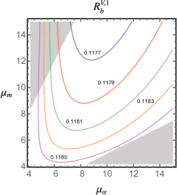
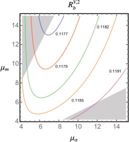
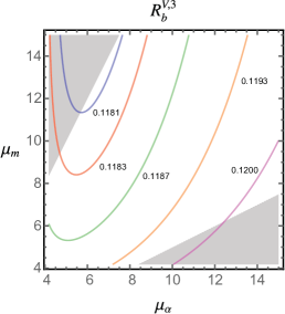
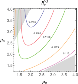
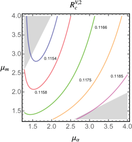
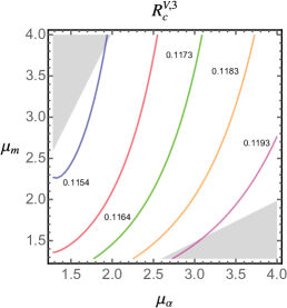
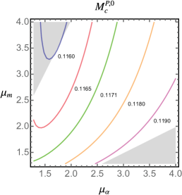
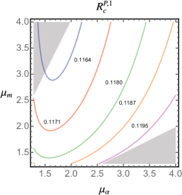
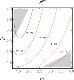
Figure 1: Contour plots for the extracted value of $\alpha_{s}^{(n_{f}=5)}(m_{Z})$ from different perturbative series at $\mathcal{O}(\alpha_{s}^{3})$, as a function of the two renormalization scales $\mu_{\alpha}$ and $\mu_{m}$. The three panels at the top show the result for the bottom vector correlator, the three in the middle (bottom) correspond to the charm vector (pseudo-scalar) correlator. For the six panels showing results for the vector correlator, the left, center and right columns correspond to $R_{q}^{V,1}$, $R_{q}^{V,2}$ and $R_{q}^{V,3}$, respectively, while for the pseudo-scalar they show $M_{c}^{P,0}$, $R_{c}^{P,1}$, and $R_{c}^{P,1}$. The shaded gray areas are excluded for $\xi=2$.

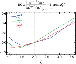
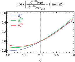
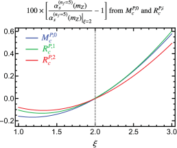
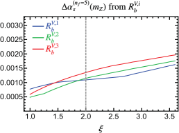
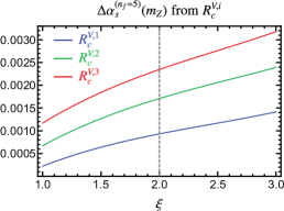
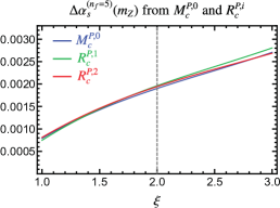
Figure 2: Dependence of the central value and perturbative uncertainty with the “trimming” parameter $\xi$, which controls how renormalization scales are varied through the constraint $1/\xi\leq\mu_{\alpha}/\mu_{m}\leq\xi$, with $\overline{m}_{q}\leq\mu_{\alpha},\mu_{m}\leq\mu_{\rm max}$ and $q=c\,(b)$ for charm (bottom). The gray, dashed, vertical lines signal our canonical choice $\xi=2$. The three panels on top correspond to how central values depend on $\xi$, shown as a percent deviation from our canonical choice for $\xi$. The three panels at the bottom show the dependence of perturbative uncertainties with $\xi$. Left, right, and middle panels correspond to bottom vector, charm vector, and charm pseudo-scalar, respectively. Blue, red and green distinguish which moment or ratio is used, as shown in the plot legends.

We continue our exploration of perturbative uncertainties drawing contour plots that show the dependence of the $\alpha_{s}^{(n_{f}=5)}(m_{Z})$ extracted value on the renormalization scales. For this exercise we do not include the gluon condensate correction and use the experimental values quoted in Table 6 for the vector correlator (using the world average value for the strong coupling), and the results of Maezawa:2016vgv shown in Table 7 for the pseudo-scalar correlator. We also use the values $\overline{m}_{c}=1.28\,$GeV, and $\overline{m}_{b}=4.18\,$GeV for the quark masses. We analyze the values of $\alpha_{s}$ as obtained from the series which include up to $\mathcal{O}(\alpha_{s}^{3})$ terms. The results for the various currents and number of flavors are collected in the three rows of Fig. 1, where different columns correspond to different ratios (except in the last row, where the leftmost panel shows the result for the $n=0$ pseudo-scalar moment) and gray shaded areas show excluded values for the choice $\xi=2$. From the plots one can conclude that, in most cases, varying the scales in a correlated way in some limited ranges may lead to serious underestimates of perturbative uncertainties. In some cases, however, a variation keeping both scales equal seems to capture most of the spread in $\alpha_{s}$ values, while in others keeping $\mu_{m}=\overline{m}_{q}$ seems also sufficient. It seems that there is no unique $1$D slice valid for all situations, and hence we conclude that an independent variation of scales is the safest procedure.

We turn now to a systematic study of the $\xi$ dependence. Since at $\mathcal{O}(\alpha_{s})$ there is no $\mu_{m}$ dependence, to estimate the perturbative uncertainty at this order we simply vary $\mu_{\alpha}$ between $\overline{m}_{q}$ and $\mu_{\rm max}$. At higher orders we once again vary $\overline{m}_{q}\leq\mu_{\alpha},\mu_{m}\leq\mu_{\rm max}$, with the constraint $1/\xi\leq\mu_{\alpha}/\mu_{m}\leq\xi$. The perturbative uncertainty is then computed as half of the difference between the maximum and minimum values of $\alpha_{s}$ in the constrained grid, while the central value is simply the average of those two. The standard choice to estimate perturbative uncertainties is to vary the argument of logarithms dividing/multiplying it by factor of $2$, which corresponds to our canonical choice $\xi=2$. Taking $\xi=1$ corresponds to the correlated variation $\mu_{\alpha}=\mu_{m}$, while very large values of $\xi$ do not impose any constraint. We show the dependence of the central value and perturbative uncertainty on the value of $\xi$ in Fig. 2. To carry out this study we do not fix the value of $\alpha_{s}$ on the charm and bottom vector-correlator experimental moments, since setting it to the world average makes the uncertainty smaller and we want to assess the effect of $\xi$ on our final uncertainty. For the bottom vector correlator, taking both scales equal yields uncertainties smaller than our canonical choice by factors of $1.4$, $2.4$, and $2.3$, for the first three ratios, respectively. For the charm-vector correlator the difference grows dramatically, with uncertainties that are smaller by factors of $3.7$, $2.5$ and $2.1$ for the first three ratios. In the pseudo-scalar case the uncertainty as a function of $\xi$ is nearly the same for all quantities considered, and the correlated estimate is $2.4$ times smaller than the default choice. The unconstrained error estimate is at most $53\%$ larger than that with $\xi=2$ for all cases. Except for values of $\xi$ close to $1$, the central value grows as $\xi$ increases, but the variation is below the percent in all cases.

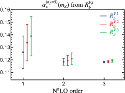
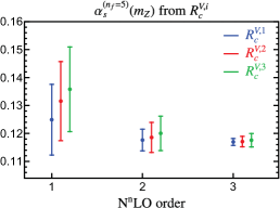
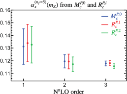
Figure 3: $\alpha_{s}^{(n_{f}=5)}(m_{Z})$ as determined from ratios of moments or $M_{c}^{P,0}$ using the corresponding perturbative series at $\mathcal{O}(\alpha_{s}^{n})$ with $n=1,2,3$ which we call NⁿLO. Panels (a), (b), and (c) show results for the bottom vector, charm vector, and charm pseudo-scalar correlators, respectively. For (a) and (b), blue, red and green correspond to $R_{q}^{V,1}$, $R_{q}^{V,2}$, and $R_{q}^{V,3}$, respectively, with $q=c,b$, while for (c) these colors correspond to $M_{c}^{P,0}$, $R_{c}^{P,1}$, and $R_{c}^{V,2}$. Error bars reflect only perturbative uncertainties, which are computed varying $\mu_{\alpha}$ and $\mu_{m}$ independently, but requiring that $0.5\leq\mu_{\alpha}/\mu_{m}\leq 2$.

We finish this section by exploring the order-by-order convergence of the extracted values of $\alpha_{s}$. Again we ignore non-perturbative effects and fix the quark masses. We also assume experimental moments have no uncertainties, such that error bars shown in this section are purely of perturbative origin. Taking the default constraint $\xi=2$ we obtain the results shown in Fig. 3. We see excellent convergence between the $\mathcal{O}(\alpha_{s}^{2})$ and $\mathcal{O}(\alpha_{s}^{3})$ determinations in all cases, while for ratios with $n>1$ there is a slight tension between the $\mathcal{O}(\alpha_{s}^{1})$ and $\mathcal{O}(\alpha_{s}^{3})$ results. This is not cause for concern since the LO extraction does not yet depend on $\mu_{m}$ and therefore should be regarded as a special case. A similar situation was found with the $\mathcal{O}(\alpha_{s}^{0})$ determination of quark masses in e.g. Ref. Dehnadi:2015fra , which was independent of $\mu_{\alpha}$. In that sense the $\mathcal{O}(\alpha_{s}^{n})$ quark-mass determination should be thought of as being of the same order as the $\mathcal{O}(\alpha_{s}^{n+1})$ strong-coupling extraction.

5 Results

In this section we present the main results of our analysis: the determination of $\alpha_{s}^{(n_{f}=5)}(m_{Z})$ using perturbative expressions at $\mathcal{O}(\alpha_{s}^{3})$ from ratios of moments for the two types of currents considered, both for charm and bottom quarks, as well as from the 0-th moment of the pseudo-scalar charm correlator. Here we include the gluon condensate correction, and take into account all relevant sources that contribute to the uncertainty. The most important contributions to the error budget are the perturbative error — due to the truncation of the series in $\alpha_{s}$, estimated through scale variation — and the experimental/lattice uncertainties (in general, experimental uncertainties in $\alpha_{s}$ from the vector correlators are larger than lattice uncertainties in $\alpha_{s}$ from the pseudo-scalar moments). To estimate the incertitude coming from the charm or bottom mass we use

$$\overline{m}_{b}=4.18\pm 0.023\,{\rm GeV}\,,\qquad\quad\overline{m}_{c}=1.28\pm 0.02\,\rm GeV\,.$$ (29)

The associated uncertainties are very small and barely contribute to the final error, since the ratios of moments we use are rather insensitive to the quark mass. Non-perturvative corrections also contribute to the error budget, but their contribution is absolutely negligible in the case of the bottom-quark based determinations, and always subleading for the charm-quark ones.

For charm-quark based determinations one could consider an additional source of uncertainty coming from matching the theories with $n_{f}=4$ and $5$ active flavors at the scale $\mu_{b}$, which by default is taken to be $\overline{m}_{b}$. The choice of $\mu_{b}$ inflicts a tiny uncertainty, which we estimate by considering $\mu_{b}=2\,\overline{m}_{b}$ and $\overline{m}_{b}/2$. Running $\alpha_{s}$ at $5$ loops (and matching accordingly at $4$ loops) it turns out to be negligibly small: $5\times 10^{-6}$. The uncertainty on the bottom mass also affects the matching relation, but the associated error is also insignificant: $1\times 10^{-5}$. These are much smaller than any other source and will no longer be mentioned.

5.1 ${\alpha_{s}}$ from ratios of vector correlators

flavor [	$n$	$\alpha_{s}^{(n_{f}=5)}(m_{Z})$	$\sigma_{\rm pert}$	$\sigma_{\rm exp}$	$\sigma_{m_{q}}$	$\sigma_{\rm np}$	$\sigma_{\rm total}$
bottom	$1$	$0.1183$	$0.0011$	$0.0089$	$0.0002$	$0.0000$	$0.0090$
	$2$	$0.1186$	$0.0011$	$0.0046$	$0.0001$	$0.0000$	$0.0048$
	$3$	$0.1194$	$0.0013$	$0.0029$	$0.0001$	$0.0000$	$0.0032$
charm	$1$	$0.1168$	$0.0010$	$0.0028$	$0.0003$	$0.0006$	$0.0030$
	$2$	$0.1168$	$0.0015$	$0.0009$	$0.0003$	$0.0007$	$0.0019$
	$3$	$0.1173$	$0.0020$	$0.0005$	$0.0003$	$0.0006$	$0.0022$

Table 8: $\alpha_{s}^{(n_{f}=5)}(m_{Z})$ determination from ratios of bottom and charm vector-correlator moments $R_{q}^{V,n}$, Eq. (8). The first column specifies the flavor content of the current, the second column shows which ratio has been used, while the third gives the central value. Fourth to seventh provide the various components of the uncertainty: scale variation ($\sigma_{\rm pert}$), experimental ($\sigma_{\rm exp}$), quark mass ($\sigma_{m_{q}}$), and gluon condensate ($\sigma_{\rm np}$), which are added in quadrature in the last column ($\sigma_{\rm tot}$).

In this section we present results based on “real” experimental data, that is, $\alpha_{s}$ extractions from ratios of vector-correlator moments, for $n_{f}=4$ and $5$. For these analyses we use the $\alpha_{s}$ dependence of the experimental moments, given in Table 6, solving the relevant equations consistently. The determinations from the charm correlator are shown graphically in Fig. 4. For comparison, the world average is shown as a faint gray band. All charmonium (and bottomonium) determinations are compatible among themselves and with the world average. Both extractions are quite robust, with rather stable central values, although the extraction from bottomonium yields somewhat larger central values than the extractions from charmonium sum rules. A detailed splitting of all sources of incertitude is given in Table 8. For both quarkonium systems we observe that perturbative uncertainties grow with $n$ (this behavior was already seen in Fig. 3), particularly for charmonium, with overall larger errors. Experimental uncertainties behave in the opposite way, decreasing as $n$ grows. This is expected since larger values of $n$ are dominated by the very precise narrow-resonance contribution. For charmonium, the larger experimental uncertainties discards the first ratio for precision extractions of $\alpha_{s}$. If the experimental error could be drastically reduced, $n=1$ could however turn into a competitive measurement, since, from the theoretical point of view, it is quite clean. For both systems there is a compensation of the two effects such that the uncertainties for $n=2$ and $n=3$ are comparable. Since the ratios $R_{q}^{V,2}$ involves the moments $M_{q}^{V,2}$ and $M_{q}^{V,3}$ their perturbative expansion is expected to be better behaved than the ones for $R_{q}^{V,3}$ which brings the contribution from $M_{q}^{V,4}$. Larger values of $n$ are disfavored since non-relativistic duality violations could start playing a non-negligible role. This is in line with the smaller perturbative uncertainty for $R_{q}^{V,2}$. Since the charm-quark based extractions have smaller errors and in the spirit of avoiding moments with large values of $n$ we take the charm $n=2$ result as the main outcome from the analysis of vector correlators:

$$\alpha_{s}^{(n_{f}=5)}(m_{Z}) =0.1168\pm(0.0015)_{\rm pert}\pm(0.0009)_{\rm exp}+(0.0006)_{\rm np}$$ (30)

$$=0.1168\pm(0.0019)_{\rm total}\,.$$

Here we do not show the $m_{c}$ uncertainty since it does not change the total error. Our result is less precise than the current world average (which has an uncertainty of $\pm 0.0011$ Tanabashi:2018oca ), being fully compatible with it: the central values differ by $0.6\,\sigma$. This value of $\alpha_{s}$ was reported, for the first time, in Ref. Boito:2019pqp .

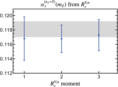
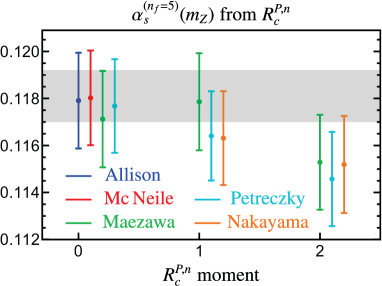
Figure 4: $\alpha_{s}^{(n_{f}=5)}(m_{Z})$ determination from ratios of charm vector-correlator (left panel) and pseudo-scalar (right panel) moments. Error bands include all sources of uncertainties added in quadrature. Panel (a) has results for the first three ratios of moments. Panel (b) has results in different colors for lattice output from various collaborations: from left to right these are Allison et al. Allison:2008xk , McNeile et al. McNeile:2010ji , Maezawa et al. Maezawa:2016vgv , Petreczky et al. Petreczky:2019ozv , and Nakayama et al. Nakayama:2016atf . $n=0$ corresponds to $R_{c}^{P,0}\equiv M_{c}^{P,0}$, while $n=1,2$ stand for $R_{c}^{P,n}$. Perturbative uncertainties are estimated trimming the grids with the default parameter $\xi=2$. The light gray area shows the current (2019) world average with its uncertainty Patrignani:2016xqp .

It is interesting to compare our final uncertainties, based on the conservative procedure of varying both scales independently, with more optimistic approaches often used in the literature. For example, if we had used a correlated scale variation with $\mu_{\alpha}=\mu_{m}$ the central value would decrease by $0.0001$, but the perturbative uncertainty would decrease by a factor of $2.12$ to $(0.0007)_{\rm pert}$, making up for a total error of only $(0.0013)_{\rm total}$. On the other hand, using a completely unconstrained grid, the central value and perturbative uncertainty grow to $0.1175\pm(0.0022)_{\rm pert}$, a $50\%$ increase in error, with a total uncertainty of $(0.0025)_{\rm total}$.

5.2 $\alpha_{s}$ from lattice data

Ref.[	$\alpha_{s}^{(n_{f}=5)}(m_{Z})$	$\sigma_{\rm pert}$	$\sigma_{\rm lattice}$	$\sigma_{m_{c}}$	$\sigma_{\rm np}$	$\sigma_{\rm total}$
Allison et al. Allison:2008xk	$0.1179$	$0.0019$	$0.0006$	$0.0003$	$0.0004$	$0.0020$
McNeile et al. McNeile:2010ji	$0.1180$	$0.0019$	$0.0005$	$0.0003$	$0.0004$	$0.0020$
Maezawa et al. Maezawa:2016vgv	$0.1171$	$0.0018$	$0.0008$	$0.0003$	$0.0004$	$0.0020$
Petreczky et al. Petreczky:2019ozv	$0.1177$	$0.0019$	$0.0005$	$0.0003$	$0.0004$	$0.0020$

Table 9: $\alpha_{s}^{(n_{f}=5)}(m_{Z})$ determination from the $n=0$ moment of the pseudo-scalar correlator $M_{c}^{P,0}$. The first column shows from which reference the lattice results are taken, the second corresponds to the central value, third to sixth provide the various component of the uncertainty: scale variation ($\sigma_{\rm pert}$), lattice ($\sigma_{\rm lattice}$), charm mass ($\sigma_{m_{c}}$) and gluon condensate ($\sigma_{\rm np}$), which are added in quadrature in the last column ($\sigma_{\rm total}$).

We turn now our attention to the pseudo-scalar Green’s function, for which “experimental” data is obtained from lattice MC simulations. A number of collaborations provide results for the same quantities, and we analyze all of those with the same theoretical expressions and identical treatment of perturbative uncertainties. The results are shown graphically in Fig. 4, using different colors for the various lattice determinations. From left to right these are: Allison et al. Allison:2008xk and McNeile et al. McNeile:2010ji (HPQCD collaboration, MILC configurations, HISQ action for light quarks and $c$-quark propagator, only $M_{c}^{P,0}$); Maezawa et al. Maezawa:2016vgv and Petreczky et al. Petreczky:2019ozv (HotQCD configurations, $2+1$ flavors plus valence c-quarks treated with the HISQ action, $M_{c}^{P,0}$ and $R_{c}^{P,n}$ with $n=1,2$); and Nakayama et al. Nakayama:2016atf (JLQCD collaboration, $2+1$ flavors plus valence c-quarks treated with the Möbius domain-wall fermion, only $R_{c}^{P,n}$ with $n=1,2$). We again include the 2019 world average as a faint gray band. The determinations from $M_{c}^{P,0}$ and $R_{c}^{P,n=1,2}$, with a complete breakdown of the uncertainty, are collected in Tables 9 and 10, respectively.

We observe that the total uncertainty is overly dominated by the truncation error, such that efforts to compute these quantities on the lattice more precisely are not warranted with our present knowledge of the perturbative series. Interestingly, perturbative errors for the pseudo-scalar correlator seem roughly independent of the moment being used. Even though all determinations are well compatible with the current world average, we observe that results from $R_{c}^{P,2}$ are slightly lower than those with $M_{c}^{P,0}$ and $R_{c}^{P,1}$. This behavior is less pronounced for the JLQCD results, which could suggest that the shift is caused by lattice results (another argument in favor of this reasoning is that for the vector correlator results with larger $n$ are higher). We also observe that $M_{c}^{P,0}$-based extractions are higher if HPQCD results are employed, although still compatible. For $R_{c}^{P,1}$-based determinations, the newest HotQCD result of Ref. Petreczky:2019ozv is in very nice agreement with the JLQCD result, although the old HotQCD determination Maezawa:2016vgv is significantly larger. Interestingly, for determinations with $R_{c}^{P,1}$ the situation is the opposite, and there is excellent agreement between JLQCD and the old HotQCD results, being again the extraction of Petreczky:2019ozv somewhat lower. All in all, the various results are compatible and there seems to be a higher density of central values around the world average. As a representative value of $\alpha_{s}$ from the pseudo-scalar lattice correlator we average the various central values from the $n=0$ moment, finding $\alpha_{s}^{(n_{f}=5)}(m_{Z})=0.1177\pm(0.0020)_{\rm total}$ .

We finish this section by comparing the perturbative uncertainties for vector and pseudo-scalar correlators with charm quarks. As expected from the analysis carried out in Sec. 2.1, the uncertainties for the pseudo-scalar correlator are larger for the $n=1,2$ ratios of moments, but for $n=3$ they become of the same order. This is in line with the findings of Ref. Dehnadi:2015fra for regular moments, and again points to the fact that the total uncertainty will not go down with more precise lattice simulations. Without $5$-loop results, possible ways of improving the accuracy are understanding the origin of the bad convergence behavior of the pseudo-scalar correlator or computing the values for ratios of the vector correlator on the lattice.

Ref.[	$n$	$\alpha_{s}^{(n_{f}=5)}(m_{Z})$	$\sigma_{\rm pert}$	$\sigma_{\rm lattice}$	$\sigma_{m_{c}}$	$\sigma_{\rm np}$	$\sigma_{\rm total}$
Maezawa et al. Maezawa:2016vgv	$1$	$0.1179$	$0.0019$	$0.0005$	$0.0003$	$0.0005$	$0.0021$
	$2$	$0.1153$	$0.0018$	$0.0004$	$0.0003$	$0.0008$	$0.0020$
Petreczky et al. Petreczky:2019ozv	$1$	$0.1164$	$0.0018$	$0.0002$	$0.0003$	$0.0006$	$0.0019$
	$2$	$0.1146$	$0.0017$	$0.0005$	$0.0003$	$0.0008$	$0.0020$
Nakayama et al. Nakayama:2016atf	$1$	$0.1163$	$0.0018$	$0.0007$	$0.0003$	$0.0006$	$0.0020$
	$2$	$0.1152$	$0.0018$	$0.0006$	$0.0003$	$0.0008$	$0.0021$

Table 10: $\alpha_{s}^{(n_{f}=5)}(m_{Z})$ determination from ratios of charm pseudo-scalar correlator moments $R_{c}^{P,n}$. The first column shows from which reference the lattice results are taken, the second which ratio has been used, the third corresponds to the central value, fourth to seventh provide the various component of the uncertainty: scale variation ($\sigma_{\rm pert}$), lattice ($\sigma_{\rm lattice}$), charm mass ($\sigma_{m_{c}}$) and gluon condensate ($\sigma_{\rm np}$), which are added in quadrature in the last column ($\sigma_{\rm total}$).

5.3 Comparison to previous lattice determinations

In this section we compare the estimates of perturbative uncertainties from the various lattice collaborations, which have a huge impact in the total uncertainty.

Ref. Allison:2008xk estimates the perturbative uncertainty on $\alpha_{s}$ from the $M_{c}^{P,0}$ moment by varying the renormalization scales setting $2\,{\rm GeV}\leq\mu_{\alpha}=\mu_{m}\leq 4\,$GeV. The result $0.1174(12)$ is quoted, with a central value in good agreement with our result in Table 9, but with a smaller error. If we use a correlated scale variation (taking the charm quark mass as the lowest scale) we obtain $0.1178\pm(0.0011)_{\rm total}$, which has a very similar total uncertainty.

Ref. McNeile:2010ji does not perform any scale variation, but estimates the uncertainty by making an educated guess for the unknown $\mathcal{O}(\alpha_{s}^{4})$ term. The $0$-th moment is used in the analysis, and value $0.1183(7)$ is quoted, which agrees well with the corresponding central value in Table 9, but has only a third of our uncertainty. Refs. Maezawa:2016vgv and Petreczky:2019ozv quote $0.11622(84)$ and $0.1159(12)$, from $M_{c}^{P,0}$ and an average of $M_{c}^{P,0}$ and $R_{c}^{P,n=1,2}$, respectively, estimating the truncation error in the same way as in McNeile:2010ji . Our uncertainties turn out to be larger because of our more conservative method to estimate perturbative errors, being our central values a bit larger. By averaging our results which use data from Petreczky:2019ozv , we obtain $0.1162$.

Ref. Nakayama:2016atf performs uncorrelated double scale variation, taking $\mu_{\alpha}=\mu_{m}\pm 1\,$GeV with $2\,{\rm GeV}\leq\min\{\mu_{\alpha},\mu_{m}\}$ and $\max\{\mu_{\alpha},\mu_{m}\}\leq 4\,$GeV. The value $0.1177\pm(0.0026)_{\rm total}$ is obtained from a combined analysis involving $M_{c}^{P,n=0,1,2}$ and their ratios. The analysis carried out in Nakayama:2016atf determines the charm quark mass and the gluon condensate, what may also contribute to a different central value. Our total uncertainty is slightly smaller than theirs, and this could be caused by their different prescription when varying the renormalization scales. If we use an unconstrained grid our total error grows to $0.0029$ and $0.0026$ for the first two ratios, the latter matching their quoted error.

5.4 Final result: fit to charm vector and pseudo-scalar moments

One can go one step further to gain precision by determining $\alpha_{s}$ from a fit to different correlators, which benefits from the fact that the experimental and lattice data are obviously uncorrelated. Since the bulk of the uncertainty comes from truncation errors, it is also crucial to realize that perturbative uncertainties from the vector and pseudo-scalar correlators are completely independent. Hence one can easily construct a $\chi^{2}$ function in which all uncertainty sources (experimental, perturbative, non-perturbative, and from the charm mass) are combined. The uncertainties due to the gluon condensate and the charm mass are correlated and we implement this into our function. For this analysis we consider two observables: $M_{c}^{P,0}$, since results from the lattice collaborations are in excellent agreement, and $R_{c}^{V,2}$, which has the smallest error among the vector moment extractions. Adding other moments to the $\chi^{2}$ would not improve the strong coupling determination, due to the strong correlations among moments from the same correlator. We take an average of all four lattice values, assigning the smallest uncertainty of the four determinations (since perturbative uncertainties overly dominate, this choice has a tiny effect on the fit outcome): $M_{c}^{P,0}=1.7054\pm 0.0053$. On the theoretical side we make a one-dimensional grid in $\alpha_{s}$, and for each value we scan in the renormalization scales as described in Sec. 4 to determine a central value and perturbative uncertainty for both the vector and pseudo-scalar moments. We make three additional grids: one setting the gluon condensate to zero and other two in which the charm mass is set to $1.3\,$GeV and $1.26\,$GeV. These extra grids are used to determine the (correlated) non-perturbative and charm-quark mass uncertainties. Following this procedure one accounts for $\alpha_{s}$-dependent theory uncertainties in a consistent way.

Our $\chi^{2}$ function takes the following form

$$\chi^{2}(\alpha_{s})=v(\alpha_{s})^{\top}\cdot[M(\alpha_{s})]^{-1}\cdot v(\alpha_{s})\,,$$ (31)

where here $\alpha_{s}\equiv\alpha_{s}^{(n_{f}=5)}(m_{Z})$ and the vector $v(\alpha_{s})$ is given by

$$v(\alpha_{s})=[\,1.7054-M_{c}^{P,0}(\alpha_{s}),1.1173-0.1130\,(\alpha_{s}-0.1181)-R_{c}^{V,2}(\alpha_{s})\,].$$ (32)

The covariance matrix that takes into account experimental and theory errors is written as

$$M(\alpha_{s})=\begin{bmatrix}0.0053^{2}+[\Delta M_{c}^{P,0}(\alpha_{s})]^{2}&m_{1,2}(\alpha_{s})\\ m_{1,2}(\alpha_{s})&0.0022^{2}+[\Delta R_{c}^{V,2}(\alpha_{s})]^{2}\end{bmatrix},$$ (33)

with theoretical errors given by ($R=R_{c}^{V,2},M_{c}^{P,0}$)

$$[\Delta R(\alpha_{s})]^{2}\equiv[\Delta R(\alpha_{s})]_{\rm pert}^{2}+[\Delta R(\alpha_{s})]_{\rm np}^{2}+[\Delta R(\alpha_{s})]_{m_{c}}^{2}\,.$$ (34)

The non-diagonal terms in Eq. (33) arise because of the correlation in the theory uncertainties due to the mass and the gluon condensate, and are written as

$$m_{1,2}(\alpha_{s})=[\Delta M_{c}^{P,0}(\alpha_{s})]_{\rm np}[\Delta R_{c}^{V,2}(\alpha_{s})]_{\rm np}+[\Delta M_{c}^{P,0}(\alpha_{s})]_{m_{c}}[\Delta R_{c}^{V,2}(\alpha_{s})]_{m_{c}}.$$ (35)

Upon the minimization of the $\chi^{2}$ function we find the main outcome of this paper

$$\alpha_{s}^{(n_{f}=5)}(m_{Z})=0.1170\pm(0.0014)_{\rm total}\,,$$ (36)

with a p-value of $26\%$. Neglecting correlations due to the gluon condensate and the charm mass the uncertainty is $0.0013$, so once again our treatment is conservative. Changing the value of $M_{c}^{P,0}$ to a weighted average (with much smaller errors from the lattice) does not change the fit outcome within four digital places. Taking instead the least precise lattice determination lowers the central value by $0.0003$, a shift much smaller than the uncertainty.

Our result is compatible with the current word average within $0.65\,\sigma$ with a smaller central value and a very similar uncertainty. As a sanity check we have also performed a standard weighted average of the individual $\alpha_{s}$ determinations from $M_{c}^{P,0}$ and $R_{c}^{V,2,}$, finding $\alpha_{s}^{(n_{f}=5)}(m_{Z})=0.1172\pm(0.0014)_{\rm total}$, in excellent agreement with Eq. (36).

6 Conclusions

In this work we have determined $\alpha_{s}$ from ratios of quarkonium correlator moments. The strategy we follow when taking the ratio is canceling the overall dependence on the heavy-quark mass, leaving only a small logarithmic dependence which is damped by two powers of the strong coupling constant. The ratio is re-expanded in $\alpha_{s}$ such that the new series has nice convergence properties. Our determination uses $\mathcal{O}(\alpha_{s}^{3})$-accurate perturbative computations, supplemented with non-perturbative corrections parameterized by the gluon condensate, which is included to $\mathcal{O}(\alpha_{s})$ precision. We compute the experimental values for the ratios of moments of charmonium, updating the computation performed in Ref. Dehnadi:2011gc , and bottomonium, using the results in Ref. Dehnadi:2015fra , but, in both cases, keeping $\alpha_{s}$ as a free parameter in the treatment of the perturbative continuum contributions, as well as in the treatment of the light-quark perturbative background in the case charmonium. It is crucial to have full control over the uncertainty correlation among moments, since there are large cancellations of errors when taking the ratios. We also analyze lattice results on ratios of the pseudo-scalar correlator.

We perform a careful study of perturbative uncertainties, and conclude that the renormalization scales of $\alpha_{s}$ and $\overline{m}_{q}$ should be varied independently in the same ranges as in Refs. Dehnadi:2011gc ; Dehnadi:2015fra . Furthermore, since the convergence parameter of the series does not show a preferred value, we do not restrict the renormalization scales based on convergence. Instead, we simply impose that the logarithm of ratios of scales is order one. This restriction ensures order-by-order convergence, while keeping uncertainties of moderate size. Our estimates are in general much more conservative than those based on educated guesses for the unknown higher order terms of the perturbative series. In that sense, our reanalyses of lattice data shows that uncertainties are overly dominated by the truncation error, such that more precise lattice simulations will not decrease the total incertitude with the present knowledge on the perturbative series.

Our main result combines experimental and lattice information on charm correlators, and reads

$$\alpha_{s}^{(n_{f}=5)}(m_{Z})=0.1170\pm(0.0014)_{\rm total}\,,$$ (37)

where the main contribution to the error comes from truncating the perturbative series. Despite our conservative perturbative error estimate, our determination is very precise. Our uncertainty could go further down if the accuracy of the experimental value for the moments of the charm vector correlator increased. On the theory side, since the perturbative error dominates, knowing the moments at $\mathcal{O}(\alpha_{s}^{4})$ would be paramount to obtain smaller uncertainties. We get a value fully compatible with the current world average with a comparable uncertainty. Our results from bottom moments, despite their smaller perturbative errors, are less precise because there is less sensitivity to $\alpha_{s}$ at larger energies even though the experimental values for the ratios are equally accurate. The situation would dramatically improve if the bottom cross section measurements in the continuum reached larger energies, and also with more precise data at threshold. In Fig. 5, we compare our main result of Eq. (36) to a selection of previous determinations from a variety of sources.

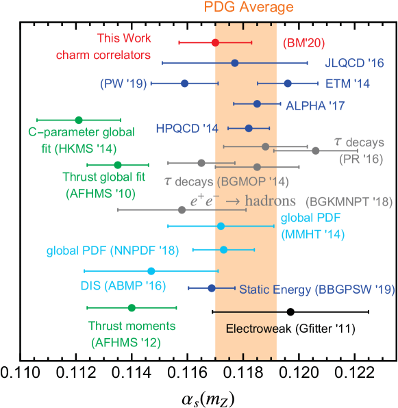
Figure 5: Comparison of our main determination of $\alpha_{s}^{(n_{f}=5)}(m_{Z})$ (red on top) with some selected determinations. Event-shape analyses at N³LL^′ + $\mathcal{O}(\alpha_{s}^{3})$: thrust and C-parameter (green) Abbate:2010xh ; Abbate:2012jh ; Hoang:2015hka ; lattice QCD HPQCD:2014aca ; Petreczky:2019ozv ; Bruno:2017gxd ; Blossier:2013ioa ; Nakayama:2016atf and static energy potential Bazavov:2019qoo (both use lattice input, in dark blue); Electroweak precision observables fits Flacher:2008zq (black); Deep Inelastic Scattering Alekhin:2017kpj and global PDF fits Ball:2018iqk ; Harland-Lang:2015nxa (light blue); and hadronic $\tau$ decays Boito:2014sta ; Pich:2016bdg and $e^{+}e^{-}\to$ hadrons Boito:2018yvl (gray). The current world average Patrignani:2016xqp is shown as a translucent orange band.

Our analysis can be extended or improved in a number of directions. On the theoretical side, as an additional sanity check on our perturbative error estimate, we could consider alternative expansions, such as taking powers of $R_{q}^{X,n}$ (and re-expanding the resulting series), or using a linearized iterative solution for $\alpha_{s}(\mu_{\alpha})$ in the same spirit of Refs. Dehnadi:2011gc ; Dehnadi:2015fra . In the same direction, one could consider analyses in which the ratio of moments is not re-expanded in powers of $\alpha_{s}$. Finally, since the renormalon associated to the pole mass cancels when taking ratios, an alternative analysis could use directly the pole mass (which appears only in logarithms). In a different direction, QED effects could can be readily accounted for, since final-state photons are included in the cross section measurements. Finally, one could consider fits to $\alpha_{s}$ using all available information (various ratios from charm and bottom correlators) included in a $\chi^{2}$ function, taking into account all correlations. Similarly, one can perform global fits to $\alpha_{s}$ and the charm and bottom quark masses.

A related analysis could use ratios of bottomonium moments for very large $n$, using NRQCD predictions for the theoretical moments, which includes resummation of Sommerfeld-enhanced terms, and, in some cases, also the logarithm of the relative velocity of the $q\bar{q}$ pair, see e.g. Refs. Hoang:2012us ; Beneke:2014pta . In this way, the experimental uncertainty would be reduced to the point of being completely negligible. The question is, of course, by how much the perturbative error grows, and if it would still make the method eligible for a precise determination of the strong coupling. Another approach to exclude the continuum from the experimental moments is using finite-energy sum rules, in which a pinched kernel suppresses quark-hadron duality violations.

In the same spirit of our present analysis, one could consider ratios of masses of bottomonium states. In Ref. Mateu:2017hlz it was shown that a simultaneous fit for the bottom quark mass and $\alpha_{s}$ was feasible, but the strong coupling was determined with large (perturbative) uncertainties. The origin of the big error was the strong correlation between the two parameters (a similar correlation was found for fits to the Cornell model in Ref. Mateu:2018zym ). The series resulting from the ratio of two bottomonium bound-state masses (having e.g. distinct principal quantum number $n$) is free from the pole-mass renormalon and depends only logarithmically on the heavy-quark mass, starting at NNLO. Therefore one a) eliminates the correlation between the two parameters, and b) has a better-behaved perturbative series. Probably one cannot use this idea in charmonium states since masses of mesons with $n=2$ are already badly described in perturbation theory.

Appendix A Renormalization group evolution for coupling and masses

Our numerical programs use an exact solution to Eqs. (17), using methods which do not rely on directly solving an ordinary differential equation such as the Runge-Kutta algorithm. For $\alpha_{s}$, the first line of Eq. (17) can be integrated as follows:

$$\log\biggl{(}\frac{\mu}{\mu_{0}}\biggr{)}=\int_{\alpha_{s}(\mu_{0})}^{\alpha_{s}(\mu)}\frac{{\rm d}\alpha}{\beta_{\rm QCD}(\alpha)}\,.$$ (38)

We analytically perform the integration using partial fractions. The root decomposition can always be performed to arbitrary precision once the number of flavors $n_{f}$ has been specified. One is then left with an ordinary equation which cannot be solved analytically beyond LL. Its solution, however, can be easily found numerically e.g. by ordinary methods (as we use in our Mathematica implementation), or using a recursive method with the LL (analytic) solution as seed (used in our python implementation). Solving the $\overline{\mathrm{MS}}$ mass RGE equation is very simple, and as usual one can decouple the $\alpha_{s}$ and $\overline{m}_{q}$ evolution of Eqs. (17) using the chain rule, finding

$$\overline{m}_{q}(\mu)=\overline{m}_{q}\,\exp\biggl{[}2\int^{\alpha_{s}(\mu)}_{\alpha_{s}\left(\overline{m}\right)}{\rm d}\alpha\frac{\gamma_{m}(\alpha)}{\beta_{\rm QCD}(\alpha)}\biggr{]}\,.$$ (39)

The integration over $\alpha_{s}$ is easily performed with the partial fraction just discussed. In our numerical codes we always use the anomalous dimensions for $\alpha_{s}$ and $\overline{m}_{q}$ at five-loop order, and the four-loop threshold condition Chetyrkin:1997un ; Chetyrkin:2005ia ; Schroder:2005hy to relate $\alpha_{s}^{(n_{f}=5)}$ and $\alpha_{s}^{(n_{f}=4)}$. We match the theories with and without an active bottom quark at the scale $\mu_{b}=\overline{m}_{b}$ using

$$\alpha_{s}^{(n_{f}=5)}(\overline{m}_{b})=\alpha_{s}^{(n_{f}=4)}(\overline{m}_{b})\biggl{\{}1+\sum_{i=2}^{4}\biggl{[}\frac{\alpha_{s}^{(n_{f}=4)}(\overline{m}_{b})}{\pi}\biggr{]}^{i}\eta_{i}\biggr{\}}\,,$$ (40)

with $\eta_{i}=\{-0.15278,-0.63345,-0.70894\}$ for $i=2,3,4$. We have checked that, with the running (matching) at five (four) loops, varying $\mu_{b}$ by factors or $2$ and $1/2$ produces a negligible uncertainty in $\alpha_{s}$, and therefore do not include this variation in our final error budget.

Appendix B Convergence properties of the series expansion of $R_{q}^{V,n}$

We study the convergence properties of the series using $V_{c}$, the parameter introduced in Ref. Dehnadi:2015fra , which is a finite-order version of Cauchy’s root convergence test. While in Ref. Dehnadi:2015fra $V_{c}$ was right-away defined on the fit parameter (in that case it was the quark mass), here we apply the method directly to the series. This is justified since the quantity we aim to determine is already the expansion parameter. Writing the series generically as $S=\sum_{i=0}s_{i}$ with $s_{i}\propto\alpha_{s}^{i}$ depending on $\mu_{\alpha}$, $\mu_{m}$ and $\overline{m}_{q}(\mu_{m})$ as

$$s_{i}\equiv\biggl{[}\frac{\alpha_{s}(\mu_{\alpha})}{\pi}\biggr{]}^{i}\sum_{j=0}^{i}\log^{j}\biggl{(}\frac{\mu}{\overline{m}_{q}(\mu_{m})}\biggr{)}\sum_{k=0}^{\max(i-1,0)}r^{X,n}_{i,j,k}\log^{k}\biggl{(}\frac{\mu_{\alpha}}{\mu_{m}}\biggr{)}\,,$$ (41)

(here we ignore non-perturbative corrections), we define

$$V_{c}=\max\Bigl{[}|s_{i}|^{\frac{1}{i+1}}\Bigr{]}_{i=1,2,3}\,.$$ (42)

The parameter $V_{c}$ depends on the tuple $(\mu_{\alpha},\mu_{m})$, and the values obtained in the grid of renormalization scales can be converted into a histogram. One can also compute the average and standard deviation of the results. These provide a measurement of the overall convergence of the perturbative expansion and the results are shown in Fig. 6, which uses a $2$-dimensional grid of $2500$ evenly distributed points. Here we use the current world average value $\alpha_{s}^{(n_{f}=5)}(m_{Z})=0.1181$. Performing the threshold matching to $4$-loop accuracy at $\mu_{m}=\overline{m}_{b}$ the world average corresponds to $\alpha_{s}^{(n_{f}=4)}(4\,{\rm GeV})=0.22865$, which is chosen as a reference value to obtain $\alpha_{s}^{(n_{f}=4)}(\mu)$ through RGE evolution. For the bottom correlator we find that the average and standard deviation for $V_{c}$ are $[\,2.02\pm 0.33,1.85\pm 0.40,1.75\pm 0.44\,]$ for the first three ratios of moments, while the corresponding histograms are shown in Fig. 6. For the charm vector correlator we obtain $[\,2.07\pm 0.47,1.99\pm 0.51,1.92\pm 0.51\,]$, with histograms shown in Fig. 6. For the pseudo-scalar correlator, we find $3.21\pm 0.66$ for the $n=0$ moment, and $[\,3.16\pm 0.58,2.44\pm 0.55\,]$ for the first two ratios, with the corresponding histograms in Fig. 6. We find values of $V_{c}$ larger than those quoted in Dehnadi:2015fra , with the maximum criterion saturated in most cases by the three-loop correction, which is larger than the lower-order ones. Histograms do not show a clear peak for any of the ratios (there is however a very prominent peaky structure for $M_{c}^{P,0}$), in clear contrast with the results of Ref. Dehnadi:2015fra . This seems to disfavor trimming grid points with $V_{c}\gg\langle V_{c}\rangle$.

Figure 6: $V_{c}$ distribution for the series corresponding to: ratios of the vector correlator for $n_{f}=5$ (bottom) [ panel (a) ]; ratios of the vector correlator for $n_{f}=4$ (charm) [ panel (b) ]; charm pseudo-scalar correlator, $0$-th moment (blue), and first two ratios (green and red). For panels (a) and (b) blue, green, and red correspond to the first, second, and third ratios of moments, respectively.

Appendix C An iterative method to extract $\alpha_{s}$ from $R_{q}^{V,n}$

In this appendix we present an algorithm to determine $\alpha_{s}$ from the perturbative series. It is based on a numerical recursive relation, and its main advantage over other traditional methods such as bisection is that one does not need to rely on intervals which should necessarily contain the solution. Let us write the series generically as

$$M_{\rm exp} =M_{0}+M_{1}\,\alpha_{s}(\mu_{\alpha})+\sum_{i=2}\,[\alpha_{s}(\mu_{\alpha})]^{i}M_{i}[\alpha_{s}(\mu_{\alpha}),\overline{m}_{q},\mu_{\alpha},\mu_{m}]\,,$$ (43)

$$M_{i}[\alpha_{s}(\mu_{\alpha}),\overline{m}_{q},\mu_{\alpha},\mu_{m}] \equiv\frac{1}{\pi^{i}}\sum_{j=0}^{i}\log^{j}\biggl{(}\frac{\mu}{\overline{m}_{q}(\mu_{m})}\biggr{)}\sum_{k=0}^{\max(i-1,0)}r^{X,n}_{i,j,k}\log^{k}\biggl{(}\frac{\mu_{\alpha}}{\mu_{m}}\biggr{)}\,,$$

where we pull the first two terms out of the sum, since their coefficients do not depend on renormalization scales. The dependence of $M_{i>1}$ on $\mu_{m}$ is through $\log(\mu_{\alpha}/\mu_{m})$ and $\overline{m}_{q}(\mu_{m})$, while the dependence on $\mu_{\alpha}$ is only through the logarithm. $M_{i>1}$ retains some (small) dependence on $\alpha_{s}(\mu_{\alpha})$ through $\overline{m}_{q}(\mu_{m})$. Our strategy is to determine $\alpha_{s}(\mu_{\alpha})$ in first place, which is afterwards evolved to a given reference scale. The leading order solution, which we denote by $\alpha^{(0)}_{s}$, is analytic and does not depend on the mass or renormalization scales. It will be used as the seed to our iterative algorithm. Solving for $\alpha_{s}(\mu_{\alpha})$ in the linear term of Eq. (43) we find the following recursive relation:

$$\alpha^{(n+1)}_{s}(\mu_{\alpha}) =\frac{M_{\rm exp}-M_{0}-\sum_{i=2}\,[\alpha^{(n)}_{s}(\mu_{\alpha})]^{i}M_{i}[\alpha^{(n)}_{s}(\mu_{\alpha}),\overline{m}_{q},\mu_{\alpha},\mu_{m}]}{M_{1}}\,,$$ (44)

$$\alpha^{(0)}_{s}(\mu_{\alpha}) =\frac{M_{\rm exp}-M_{0}}{M_{1}}\,,$$

where the superscript $(n)$ denotes the iteration number. The procedure is repeated until the numerical value of $\alpha_{s}(\mu_{\alpha})$ does not change within $15$ decimal places. While we implement this algorithm into our python code, its Mathematica counterpart uses built-in functions to find roots of equations. Equation (44) can be trivially modified to account for the gluon condensate correction, that is included in our final analysis.

References

- (1) A. Pich, J. Rojo, R. Sommer and A. Vairo, Determining the strong coupling: status and challenges, PoS Confinement2018 (2018) 035, [1811.11801].
- (2) G. P. Salam, The strong coupling: a theoretical perspective, in From My Vast Repertoire …: Guido Altarelli’s Legacy (A. Levy, S. Forte and G. Ridolfi, eds.), pp. 101–121. 2019. 1712.05165. DOI.
- (3) B. Dehnadi, A. H. Hoang, V. Mateu and S. M. Zebarjad, Charm Mass Determination from QCD Charmonium Sum Rules at Order , JHEP 09 (2013) 103, [1102.2264].
- (4) G. Corcella and A. H. Hoang, Uncertainties in the bottom quark mass from relativistic sum rules, Phys. Lett. B554 (2003) 133–140, [hep-ph/0212297].
- (5) B. Dehnadi, A. H. Hoang and V. Mateu, Bottom and Charm Mass Determinations with a Convergence Test, JHEP 08 (2015) 155, [1504.07638].
- (6) M. A. Shifman, A. I. Vainshtein and V. I. Zakharov, QCD and Resonance Physics. Sum Rules, Nucl. Phys. B147 (1979) 385–447.
- (7) M. A. Shifman, A. I. Vainshtein and V. I. Zakharov, QCD and Resonance Physics: Applications, Nucl. Phys. B147 (1979) 448–518.
- (8) HPQCD collaboration, I. Allison et al., High-Precision Charm-Quark Mass from Current-Current Correlators in Lattice and Continuum QCD, Phys. Rev. D78 (2008) 054513, [0805.2999].
- (9) C. McNeile, C. T. H. Davies, E. Follana, K. Hornbostel and G. P. Lepage, High-Precision c and b Masses, and QCD Coupling from Current-Current Correlators in Lattice and Continuum QCD, Phys. Rev. D82 (2010) 034512, [1004.4285].
- (10) Y. Maezawa and P. Petreczky, Quark masses and strong coupling constant in 2+1 flavor QCD, Phys. Rev. D94 (2016) 034507, [1606.08798].
- (11) P. Petreczky and J. H. Weber, Strong coupling constant and heavy quark masses in (2+1)-flavor QCD, Phys. Rev. D100 (2019) 034519, [1901.06424].
- (12) K. Nakayama, B. Fahy and S. Hashimoto, Short-distance charmonium correlator on the lattice with Möbius domain-wall fermion and a determination of charm quark mass, Phys. Rev. D94 (2016) 054507, [1606.01002].
- (13) D. Boito and V. Mateu, Precise determination from charmonium sum rules, 1912.06237.
- (14) A. O. G. Kallen and A. Sabry, Fourth order vacuum polarization, Kong. Dan. Vid. Sel. Mat. Fys. Med. 29N17 (1955) 1–20.
- (15) K. G. Chetyrkin, J. H. Kuhn and M. Steinhauser, Heavy quark vacuum polarization to three loops, Phys. Lett. B371 (1996) 93–98, [hep-ph/9511430].
- (16) K. G. Chetyrkin, J. H. Kuhn and M. Steinhauser, Three loop polarization function and corrections to the production of heavy quarks, Nucl. Phys. B482 (1996) 213–240, [hep-ph/9606230].
- (17) R. Boughezal, M. Czakon and T. Schutzmeier, Four-loop tadpoles: Applications in QCD, Nucl. Phys. Proc. Suppl. 160 (2006) 160–164, [hep-ph/0607141].
- (18) M. Czakon and T. Schutzmeier, Double fermionic contributions to the heavy-quark vacuum polarization, JHEP 07 (2008) 001, [0712.2762].
- (19) A. Maier, P. Maierhofer and P. Marquard, Higher Moments of Heavy Quark Correlators in the Low Energy Limit at , Nucl. Phys. B797 (2008) 218–242, [0711.2636].
- (20) A. Maier and P. Marquard, Validity of Padé approximations in vacuum polarization at three- and four-loop order, Phys. Rev. D97 (2018) 056016, [1710.03724].
- (21) K. G. Chetyrkin, J. H. Kuhn and C. Sturm, Four-loop moments of the heavy quark vacuum polarization function in perturbative QCD, Eur. Phys. J. C48 (2006) 107–110, [hep-ph/0604234].
- (22) R. Boughezal, M. Czakon and T. Schutzmeier, Charm and bottom quark masses from perturbative QCD, Phys. Rev. D74 (2006) 074006, [hep-ph/0605023].
- (23) C. Sturm, Moments of Heavy Quark Current Correlators at Four-Loop Order in Perturbative QCD, JHEP 09 (2008) 075, [0805.3358].
- (24) A. Maier, P. Maierhofer and P. Marqaurd, The second physical moment of the heavy quark vector correlator at , Phys. Lett. B669 (2008) 88–91, [0806.3405].
- (25) A. Maier, P. Maierhofer, P. Marquard and A. V. Smirnov, Low energy moments of heavy quark current correlators at four loops, Nucl. Phys. B824 (2010) 1–18, [0907.2117].
- (26) A. H. Hoang, V. Mateu and S. Mohammad Zebarjad, Heavy Quark Vacuum Polarization Function at and , Nucl. Phys. B813 (2009) 349–369, [0807.4173].
- (27) Y. Kiyo, A. Maier, P. Maierhofer and P. Marquard, Reconstruction of heavy quark current correlators at , Nucl. Phys. B823 (2009) 269–287, [0907.2120].
- (28) D. Greynat and S. Peris, Resummation of Threshold, Low- and High-Energy Expansions for Heavy-Quark Correlators, Phys. Rev. D82 (2010) 034030, [1006.0643].
- (29) D. Greynat, P. Masjuan and S. Peris, Analytic Reconstruction of heavy-quark two-point functions at , Phys. Rev. D85 (2012) 054008, [1104.3425].
- (30) S. A. Larin and J. A. M. Vermaseren, The Three loop QCD Beta function and anomalous dimensions, Phys. Lett. B303 (1993) 334–336, [hep-ph/9302208].
- (31) T. van Ritbergen, J. A. M. Vermaseren and S. A. Larin, The four-loop beta function in quantum chromodynamics, Phys. Lett. B400 (1997) 379–384, [hep-ph/9701390].
- (32) J. A. M. Vermaseren, S. A. Larin and T. van Ritbergen, The 4-loop quark mass anomalous dimension and the invariant quark mass, Phys. Lett. B405 (1997) 327–333, [hep-ph/9703284].
- (33) K. G. Chetyrkin, Quark mass anomalous dimension to , Phys. Lett. B404 (1997) 161–165, [hep-ph/9703278].
- (34) M. Czakon, The Four-loop QCD beta-function and anomalous dimensions, Nucl. Phys. B710 (2005) 485–498, [hep-ph/0411261].
- (35) P. A. Baikov, K. G. Chetyrkin and J. H. Kühn, Quark Mass and Field Anomalous Dimensions to , JHEP 10 (2014) 076, [1402.6611].
- (36) T. Luthe, A. Maier, P. Marquard and Y. Schröder, Five-loop quark mass and field anomalous dimensions for a general gauge group, JHEP 01 (2017) 081, [1612.05512].
- (37) T. Luthe, A. Maier, P. Marquard and Y. Schroder, The five-loop Beta function for a general gauge group and anomalous dimensions beyond Feynman gauge, JHEP 10 (2017) 166, [1709.07718].
- (38) V. Mateu and P. G. Ortega, Bottom and Charm Mass determinations from global fits to bound states at N3LO, JHEP 01 (2018) 122, [1711.05755].
- (39) G. Rossum, Python reference manual, tech. rep., Amsterdam, The Netherlands, The Netherlands, 1995.
- (40) Wolfram Research, Inc., Mathematica, Version 12.0. Wolfram Research, Inc., Champaign, IL, 2019.
- (41) V. A. Novikov et al., Charmonium and Gluons: Basic Experimental Facts and Theoretical Introduction, Phys. Rept. 41 (1978) 1–133.
- (42) P. A. Baikov, V. A. Ilyin and V. A. Smirnov, Gluon condensate fit from the two loop correction to the coefficient function, Phys. Atom. Nucl. 56 (1993) 1527–1530.
- (43) S. Narison and R. Tarrach, Higher dimension renormalization group invariant vacuum condensates in Quantum Chromodynamics, Phys. Lett. B125 (1983) 217.
- (44) B. L. Ioffe, QCD at low energies, Prog. Part. Nucl. Phys. 56 (2006) 232–277, [hep-ph/0502148].
- (45) K. Chetyrkin, J. H. Kuhn, A. Maier, P. Maierhofer, P. Marquard, M. Steinhauser et al., Precise Charm- and Bottom-Quark Masses: Theoretical and Experimental Uncertainties, Theor. Math. Phys. 170 (2012) 217–228, [1010.6157].
- (46) D. J. Broadhurst et al., Two loop gluon condensate contributions to heavy quark current correlators: Exact results and approximations, Phys. Lett. B329 (1994) 103–110, [hep-ph/9403274].
- (47) Particle Data Group collaboration, C. Patrignani et al., Review of Particle Physics, Chin. Phys. C40 (2016) 100001.
- (48) J. H. Kuhn, M. Steinhauser and C. Sturm, Heavy quark masses from sum rules in four-loop approximation, Nucl. Phys. B778 (2007) 192–215, [hep-ph/0702103].
- (49) Particle Data Group collaboration, K. Nakamura et al., Review of particle physics, J. Phys. G37 (2010) 075021.
- (50) K. G. Chetyrkin, J. H. Kuhn, A. Maier, P. Maierhofer, P. Marquard, M. Steinhauser et al., Addendum to “Charm and bottom quark masses: An update”, Phys. Rev. D96 (2017) 116007, [1710.04249].
- (51) Particle Data Group collaboration, M. Tanabashi et al., Review of Particle Physics, Phys. Rev. D98 (2018) 030001.
- (52) BES collaboration, J. Z. Bai et al., Measurement of the Total Cross Section for Hadronic Production by Annihilation at Energies between 2.6-5 GeV, Phys. Rev. Lett. 84 (2000) 594–597, [hep-ex/9908046].
- (53) BES collaboration, J. Z. Bai et al., Measurements of the Cross Section for hadrons at Center-of-Mass Energies from 2 to 5 GeV, Phys. Rev. Lett. 88 (2002) 101802, [hep-ex/0102003].
- (54) BES collaboration, M. Ablikim et al., Measurement of Cross Sections for and Production in Annihilation at GeV, Phys. Lett. B603 (2004) 130–137, [hep-ex/0411013].
- (55) BES collaboration, M. Ablikim et al., Measurements of the cross sections for hadrons at 3.650-GeV, 3.6648-GeV, 3.773-GeV and the branching fraction for non , Phys. Lett. B641 (2006) 145–155, [hep-ex/0605105].
- (56) M. Ablikim et al., Measurements of the continuum and values in annihilation in the energy region between 3.650-GeV and 3.872-GeV, Phys. Rev. Lett. 97 (2006) 262001, [hep-ex/0612054].
- (57) BES Bollaboration collaboration, M. Ablikim et al., value measurements for annihilation at 2.60, 3.07 and 3.65 GeV, Phys. Lett. B677 (2009) 239–245, [0903.0900].
- (58) A. Osterheld et al., Measurements of total hadronic and inclusive cross-sections in annihilations between GeV and GeV, SLAC-PUB-4160 (1986) .
- (59) C. Edwards et al., Hadron production in annihilation from GeV to GeV, SLAC-PUB-5160 (1990) .
- (60) CLEO collaboration, R. Ammar et al., Measurement of the total cross section for hadrons at GeV, Phys. Rev. D57 (1998) 1350–1358, [hep-ex/9707018].
- (61) CLEO collaboration, D. Besson et al., Observation of New Structure in the Annihilation Cross-Section Above B Threshold, Phys. Rev. Lett. 54 (1985) 381.
- (62) CLEO collaboration, D. Besson et al., Measurement of the Total Hadronic Cross Section in Annihilations below 10.56 GeV, Phys. Rev. D76 (2007) 072008, [0706.2813].
- (63) CLEO collaboration, D. Cronin-Hennessy et al., Measurement of Charm Production Cross Sections in Annihilation at Energies between 3.97 and 4.26 GeV, Phys. Rev. D80 (2009) 072001, [0801.3418].
- (64) A. E. Blinov et al., The Measurement of R in annihilation at center-of- mass energies between GeV and GeV, Z. Phys. C70 (1996) 31–38.
- (65) L. Criegee and G. Knies, Review of experiments with PLUTO from GeV to GeV, Phys. Rept. 83 (1982) 151.
- (66) G. S. Abrams et al., Measurement of the parameters of the resonance, Phys. Rev. D21 (1980) 2716.
- (67) K. Hagiwara, A. D. Martin, D. Nomura and T. Teubner, Predictions for g-2 of the muon and , Phys. Rev. D69 (2004) 093003, [hep-ph/0312250].
- (68) V. V. Anashin et al., Measurement of and between 3.12 and 3.72 GeV at the KEDR detector, Phys. Lett. B753 (2016) 533–541, [1510.02667].
- (69) V. V. Anashin et al., Measurement of between 1.84 and 3.05 GeV at the KEDR detector, Phys. Lett. B770 (2017) 174–181, [1610.02827].
- (70) KEDR collaboration, V. V. Anashin et al., Precise measurement of and between 1.84 and 3.72 GeV at the KEDR detector, Phys. Lett. B788 (2019) 42–51, [1805.06235].
- (71) iminuit team, “iminuit – a python interface to minuit.” https://github.com/scikit-hep/iminuit.
- (72) F. James and M. Roos, Minuit – a system for function minimization and analysis of the parameter errors and correlations, Comput. Phys. Commun. 10 (Jul, 1975) 343–367.
- (73) S. Groote and A. A. Pivovarov, Low-energy gluon contributions to the vacuum polarization of heavy quarks, JETP Lett. 75 (2002) 221, [hep-ph/0103047].
- (74) BABAR Collaboration collaboration, B. Aubert et al., Measurement of the cross section between GeV and GeV, Phys.Rev.Lett. 102 (2009) 012001, [0809.4120].
- (75) S. Zafeiropoulos, P. Boucaud, F. De Soto, J. Rodríguez-Quintero and J. Segovia, Strong Running Coupling from the Gauge Sector of Domain Wall Lattice QCD with Physical Quark Masses, Phys. Rev. Lett. 122 (2019) 162002, [1902.08148].
- (76) ETM collaboration, B. Blossier, P. Boucaud, M. Brinet, F. De Soto, V. Morenas, O. Pene et al., High statistics determination of the strong coupling constant in Taylor scheme and its OPE Wilson coefficient from lattice QCD with a dynamical charm, Phys. Rev. D89 (2014) 014507, [1310.3763].
- (77) R. Abbate, M. Fickinger, A. H. Hoang, V. Mateu and I. W. Stewart, Thrust at N3LL with Power Corrections and a Precision Global Fit for , Phys. Rev. D83 (2011) 074021, [1006.3080].
- (78) R. Abbate, M. Fickinger, A. H. Hoang, V. Mateu and I. W. Stewart, Precision Thrust Cumulant Moments at N3LL, Phys. Rev. D86 (2012) 094002, [1204.5746].
- (79) A. H. Hoang, D. W. Kolodrubetz, V. Mateu and I. W. Stewart, Precise determination of from the -parameter distribution, Phys. Rev. D91 (2015) 094018, [1501.04111].
- (80) HPQCD collaboration, B. Chakraborty, C. T. H. Davies, B. Galloway, P. Knecht, J. Koponen, G. C. Donald et al., High-precision quark masses and QCD coupling from lattice QCD, Phys. Rev. D91 (2015) 054508, [1408.4169].
- (81) ALPHA collaboration, M. Bruno, M. Dalla Brida, P. Fritzsch, T. Korzec, A. Ramos, S. Schaefer et al., QCD Coupling from a Nonperturbative Determination of the Three-Flavor Parameter, Phys. Rev. Lett. 119 (2017) 102001, [1706.03821].
- (82) TUMQCD collaboration, A. Bazavov, N. Brambilla, X. Garcia i Tormo, P. Petreczky, J. Soto, A. Vairo et al., Determination of the QCD coupling from the static energy and the free energy, Phys. Rev. D100 (2019) 114511, [1907.11747].
- (83) H. Flacher et al., Gfitter - Revisiting the Global Electroweak Fit of the Standard Model and Beyond, Eur. Phys. J. C60 (2009) 543–583, [0811.0009].
- (84) S. Alekhin, J. Blümlein, S. Moch and R. Placakyte, Parton distribution functions, , and heavy-quark masses for LHC Run II, Phys. Rev. D96 (2017) 014011, [1701.05838].
- (85) NNPDF collaboration, R. D. Ball, S. Carrazza, L. Del Debbio, S. Forte, Z. Kassabov, J. Rojo et al., Precision determination of the strong coupling constant within a global PDF analysis, Eur. Phys. J. C78 (2018) 408, [1802.03398].
- (86) L. A. Harland-Lang, A. D. Martin, P. Motylinski and R. S. Thorne, Uncertainties on in the MMHT2014 global PDF analysis and implications for SM predictions, Eur. Phys. J. C75 (2015) 435, [1506.05682].
- (87) D. Boito, M. Golterman, K. Maltman, J. Osborne and S. Peris, Strong coupling from the revised ALEPH data for hadronic decays, Phys. Rev. D91 (2015) 034003, [1410.3528].
- (88) A. Pich and A. Rodríguez-Sánchez, Determination of the QCD coupling from ALEPH decay data, Phys. Rev. D94 (2016) 034027, [1605.06830].
- (89) D. Boito, M. Golterman, A. Keshavarzi, K. Maltman, D. Nomura, S. Peris et al., Strong coupling from hadrons below charm, Phys. Rev. D98 (2018) 074030, [1805.08176].
- (90) A. Hoang, P. Ruiz-Femenia and M. Stahlhofen, Renormalization Group Improved Bottom Mass from Upsilon Sum Rules at NNLL Order, JHEP 10 (2012) 188, [1209.0450].
- (91) M. Beneke, A. Maier, J. Piclum and T. Rauh, The bottom-quark mass from non-relativistic sum rules at NNNLO, Nucl. Phys. B891 (2015) 42–72, [1411.3132].
- (92) V. Mateu, P. G. Ortega, D. R. Entem and F. Fernández, Calibrating the Naïve Cornell Model with NRQCD, Eur. Phys. J. C79 (2019) 323, [1811.01982].
- (93) K. G. Chetyrkin, B. A. Kniehl and M. Steinhauser, Decoupling relations to and their connection to low-energy theorems, Nucl. Phys. B510 (1998) 61–87, [hep-ph/9708255].
- (94) K. G. Chetyrkin, J. H. Kuhn and C. Sturm, QCD decoupling at four loops, Nucl. Phys. B744 (2006) 121–135, [hep-ph/0512060].
- (95) Y. Schroder and M. Steinhauser, Four-loop decoupling relations for the strong coupling, JHEP 01 (2006) 051, [hep-ph/0512058].