Implications of Milky Way Substructures for the Nature of Dark Matter

Abstract

We study how the indirect observation of dark matter substructures in the Milky Way, using recent stellar stream studies, translates into constraints for different dark matter models. Particularly, we use the measured number of dark subhalos in the mass range $10^{7}$–$10^{9}\text{M}_{\odot}$ to constrain modifications of the subhalo mass function compared to the cold dark matter scenario. We obtain the lower bounds $m_{\text{WDM}}>$3.2\text{\,}\mathrm{k}\mathrm{e}\mathrm{V}$$ and $m_{\text{FDM}}>$5.2\text{\times}{10}^{-21}\text{\,}\mathrm{e}\mathrm{V}$$ on the warm dark matter and fuzzy dark matter particle mass, respectively. When dark matter is coupled to a dark radiation bath, we find that kinetic decoupling must take place at temperatures higher than $T_{\text{kd}}>$0.7\text{\,}\mathrm{k}\mathrm{e}\mathrm{V}$$. We also discuss future prospects of stellar stream observations.

I Introduction

Unveiling the elusive nature of dark matter (DM) has proven to be an extremely difficult endeavor Jungman et al. (1996); Bertone et al. (2005). The DM candidate particle masses span more than 75 orders of magnitude while its feeble non-gravitational interactions with the Standard Model, if they exist at all, are strongly model dependent and have so far evaded detection. In the absence of any reliable signal of direct or indirect detection, the main source of information to constrain the DM properties are cosmological and astrophysical observations.

The cold dark matter (CDM) paradigm has been remarkably successful in explaining the large scale structure of the Universe. Yet there are several discrepancies between observations and CDM only numerical simulations at smaller scales, that is, galactic and subgalactic scales. These include the “missing satellite” problem Klypin et al. (1999); Moore et al. (1999a), the “too-big-to-fail” problem Boylan-Kolchin et al. (2011, 2012); Garrison-Kimmel et al. (2014); Papastergis et al. (2015); Kaplinghat et al. (2019), the core-cusp problem Moore (1994); Flores and Primack (1994); Burkert (1996); Moore et al. (1999b); van den Bosch and Swaters (2001); de Blok et al. (2001), the plane of satellites problem Pawlowski et al. (2013) and the diversity problem Oman et al. (2015). It is unknown whether these small-scale discrepancies might be alleviated by baryonic physics or if they arise from an inadequacy of the standard paradigm (for recent reviews see e.g. Kuhlen et al. (2012); Tulin and Yu (2018); Bullock and Boylan-Kolchin (2017)). The latter solution has motivated alternative DM scenarios, such as warm dark matter (WDM), fuzzy dark matter (FDM) and self-interacting dark matter (SIDM) models.

In this respect, the abundance of DM substructure can provide valuable information about the nature of DM. Many DM models predict abundances of low-mass dark subhalos that lie much below the CDM prediction. Such models are WDM Bode et al. (2001); Colin et al. (2000), FDM Hu et al. (2000); Schive et al. (2016); Marsh (2016a); Hui et al. (2017); Du et al. (2017) and those SIDM scenarios in which DM interacts with a dark radiation bath Cyr-Racine and Sigurdson (2013); Vogelsberger et al. (2012, 2016); Huo et al. (2018). Other models, such as primordial black hole (PBH) DM Hawking (1971); Carr and Hawking (1974); Carr et al. (2016), may, instead, enhance small scale structure due to the PBH induced shot noise Murgia et al. (2019); Hütsi et al. (2019); Inman and Ali-Haïmoud (2019).

Observables such as gravitational lensing Vegetti et al. (2010, 2012); Hezaveh et al. (2016a, b); Díaz Rivero et al. (2018); Brehmer et al. (2019); Hsueh et al. (2019); Alexander et al. (2019a); Gilman et al. (2020), the Lyman-$\alpha$ forest Croft et al. (1998, 2002); Viel et al. (2013); Seljak et al. (2006); Boyarsky et al. (2009); Iršič et al. (2017); Palanque-Delabrouille et al. (2019) and stellar dynamics Ibata et al. (2002); Yoon et al. (2011); Carlberg (2012); Feldmann and Spolyar (2015); Bovy et al. (2017); Erkal et al. (2016); Buschmann et al. (2018); Kim et al. (2017); Escudero et al. (2018); Jethwa et al. (2018); Marsh and Niemeyer (2019); Banik et al. (2018); Schive et al. (2019); Nadler et al. (2019); Bonaca et al. (2019); Banik et al. (2019a) can be used to experimentally distinguish between these DM scenarios. The analysis of fluctuations in the stellar density of tidal streams in ref. Banik et al. (2019a), used to indirectly measure the number of dark subhalos in the Milky Way in the mass range $10^{7}$–$10^{9}\text{M}_{\odot}$, can be used to constrain DM models. The case of WDM has been studied in ref. Banik et al. (2019b). Here, we generalize this analysis to other DM scenarios and discuss future prospects for similar studies. We find that they may improve the bounds from lensing and Lyman-$\alpha$, which we review.

We discuss halo substructure for different DM scenarios in a unified framework. To this end we show that the modification of the subhalo mass function (SHMF), compared to the CDM case, can be approximated by a universal fitting form for a broad range of DM models. Given the theoretical and astrophysical uncertainties it is possible to constrain the scale at which the SHMF is suppressed, but not the specific shape of the suppression factor. This implies that it is not yet possible to observationally discriminate between modified DM scenarios using stellar streams. Nevertheless, the current constraints are on the verge of clashing with the modified DM explanation of small scale discrepancies. Therefore, future observations have the potential to test the validity of the CDM paradigm.

The paper is structured as follows. In section II, we review the SHMF for different DM models. Section III describes different techniques used to constrain the SHMF. It further includes a summary of current bounds on distinct DM models. In section IV we present future prospects and we conclude in section V. We use natural units $\hbar=c=1$.

II Halo substructure in modified DM scenarios

The SHMF for WDM, FDM and SIDM models is suppressed for small halo masses when compared to the prediction for a CDM Universe. The deviation can be approximately parametrized by

$$\frac{dn_{\rm sub}}{dM}=f\left[1+\left(\frac{M_{\text{cut}}}{M}\right)^{\alpha}\right]^{-\beta}\left(\frac{dn_{\rm sub}}{dM}\right)_{\text{CDM}},$$ (1)

where $M_{\text{cut}}$, $\alpha$, $\beta$ and $f$ are free parameters that depend on the DM model under consideration. This fitting form generalizes the one proposed in refs. Schneider et al. (2012); Banik et al. (2019a) which corresponds to the case $\alpha=1$ (see appendix A for further discussion). The survival fraction $f$ takes into account baryonic effects, such as tidal interactions with the central galaxy’s potential, that reduce the number of subhalos with respect to the DM only case. In the CDM scenario, $f$ is expected to take values in the range 0.1 - 0.5 D’Onghia et al. (2010); Sawala et al. (2017); Garrison-Kimmel et al. (2017). Although the effect of baryonic tidal stripping and disruption is yet to be studied in detail, it can be neglected for the purpose of obtaining conservative bounds on $M_{\text{cut}}$, as it would reduce the number of subhalos with masses around $M_{\text{cut}}$. In order to better separate the scale of suppression and the shape of the suppression factor, we also define the related mass scale $M_{\nicefrac{{1}}{{2}}}\equiv M_{\text{cut}}/\sqrt[\alpha]{2^{1/\beta}-1}$, which gives the point at which the abundance of subhalos is suppressed by a factor of $1/2$ with respect to the CDM case. Constraints in the $(f,M_{\nicefrac{{1}}{{2}}})$ plane for different shapes of the suppression factor (1) are depicted in figure 1. We remark that eq. (1) also contains the exponential suppression factor, which is obtained in the limit $\beta\to\infty$ with $M_{\nicefrac{{1}}{{2}}}$ kept fixed.

Another important mass scale related to the suppression of the linear power spectrum of density fluctuations is the half-mode mass

$$M_{\text{hm}}\equiv\frac{4}{3}\pi\rho_{b}\left(\frac{\pi}{k_{\text{hm}}}\right)^{3},$$ (2)

where $\rho_{b}=2.8\times 10^{11}\Omega_{m}h^{2}\,{\rm M_{\odot}/Mpc^{3}}$ is the background matter density and $k_{\text{hm}}$ is the wavenumber for which the linear power spectrum is suppressed by a factor of $1/2$ with respect to the CDM case. We stress that $M_{\nicefrac{{1}}{{2}}}$, $M_{\text{cut}}$ and $M_{\text{hm}}$ are different mass scales. The suppression of the SHMF can be related to the modified linear spectrum via the adimensional parameter $\gamma=M_{\text{cut}}/M_{\text{hm}}$.

The simplified ansatz (1) can fail in the regime where the SHMF is strongly suppressed with respect to the CDM case. As shown in appendix A a better fit can be obtained by allowing for a weak dependence in the subhalo mass. In addition, $f$ might not be constant in the mass range under study (i.e. $10^{7}-10^{9}\,{\rm M_{\odot}}$) D’Onghia et al. (2010) and can depend on the DM model under consideration since subhalos with shallower cores are more prone to depletion Errani and Peñarrubia (2019). However, as the constraints on the abundance of subhalos are determined mainly by the suppression around the scale $M_{\nicefrac{{1}}{{2}}}$, modifications to the SHMF much below this mass scale, e.g. additional peaks as seen in FDM studies Du et al. (2017), do not affect our conclusions.

In the following we will review the SHMF in eq. (1) for different DM models.

Warm dark matter

Warm DM particles posses a non-negligible velocity dispersion. This would suppress primordial matter fluctuations at small scales. The values $\alpha=1$, $\gamma=2.7$ and $\beta=0.99$ have been found in ref. Lovell et al. (2014) for a thermal WDM relic. However, other values for these two parameters have been suggested Schneider et al. (2012); Lovell et al. (2014). For this reason, in appendix A we further investigate substructure suppression in WFM (and FDM) models using the analytic formalism of Schneider (2015) which provides a rather generic framework for treating models with reduced small-scale power.

The scale $M_{\text{hm}}$ is controlled by the mass $m_{\text{WDM}}$ of the WDM particle through Viel et al. (2005):

$$M_{\rm hm}\simeq 2\times 10^{10}{\rm M_{\odot}}\left(\frac{m_{\text{WDM}}}{$\mathrm{k}\mathrm{e}\mathrm{V}$}\right)^{-3.33}\\ \times\left(\frac{\Omega_{m}}{0.30}\right)\left(\frac{\Omega_{\text{WDM}}}{0.25}\right)^{0.33}\left(\frac{h}{0.7}\right)^{2.66},$$ (3)

where $\Omega_{m}$ and $\Omega_{\text{WDM}}$ are the contributions of matter and WDM to the density parameter, respectively, and $h$ is the dimensionless Hubble constant.

Fuzzy dark matter

FDM is a theoretically well-motivated scenario where DM is constituted by ultralight scalars such as axion-like particles or moduli fields Marsh (2016a); Hui et al. (2017). In this scenario, halos with masses below some sharp cutoff scale are strongly suppressed due to quantum pressure effects Hu et al. (2000); Marsh (2016b). The effect on the SHMF can be approximated by eq. (1) with a relatively high value of $\beta$, with $\alpha=1.1$ and $\beta=2.2$ Schive et al. (2016). The cutoff scale is dictated in this case by the particle mass $m_{\text{FDM}}$ Hui et al. (2017),

$$M_{\text{hm}}\simeq 4.6\times 10^{10}\text{M}_{\odot}\left(\frac{\Omega_{\text{FDM}}}{0.25}\right)\left(\frac{${10}^{-22}\text{\,}\mathrm{e}\mathrm{V}$}{m_{\text{FDM}}}\right)^{4/3}.$$ (4)

In appendix A we give a slight modification of the above formula (see eq. (18)). Constraints on $m_{\text{FDM}}$ obtained by using eq. (18) differ by less than 5% compared to those obtained by using eq. (4).

We can further use the quantum nature of FDM sub-halos to set constraints on the FDM mass. Particularly, FDM particles inside the solitonic core of a subhalo, that is orbiting a host galaxy, have a finite probability of tunneling the subhalo’s self-gravitational potential. Thus, after a finite time the subhalo might be completely disrupted Hui et al. (2017). The characteristic timescale $\tau\equiv M_{\rm sub}/\dot{M}_{\rm sub}$ for the depletion of a FDM subhalo, with mass $M_{\rm sub}$ and solitonic central density $\rho_{c}$, can be expressed as $\tau=T_{\rm orb}C^{-1}(\rho_{c}/\bar{\rho}_{\rm host})$ where $\bar{\rho}_{\rm host}$ is the average density of the host within the orbital radius, $T_{\rm orb}$ is the orbital period and $C$ is an invertible function determined from the Schrödinger-Poisson system for FDM halo Hui et al. (2017); Du et al. (2018). Therefore, FDM subhalos with a solitonic central density

$$\rho_{c}<C(N_{\rm orb})\bar{\rho}_{\rm host}$$ (5)

have lost a significant amount of its mass after having completed more than $N_{\rm orb}$ circular orbits around its host halo. We approximate $C(N_{\rm orb})$ with the analytic fitting form given in ref. Du et al. (2018).

The central density of the solitonic core satisfies $\rho_{c}\leq 0.0044(Gm_{\rm FDM}^{2})^{3}M^{4}$ Hui et al. (2017). Therefore, observations of FDM subhalos with a mass $M_{\rm sub}$ imply the following constraint for the FDM mass:

$$m_{\text{FDM}}\geq${10}^{-22}\text{\,}\mathrm{e}\mathrm{V}$\left[\frac{M_{\rm sub}}{10^{9}\,{\rm\text{M}_{\odot}}}\right]^{-2/3}\left[\frac{\bar{\rho}_{\text{host}}(r)}{7.05\,{\rm\text{M}_{\odot}}$\mathrm{p}\mathrm{c}^{-3}$}\right]^{1/6}\\ \times\left[C(N_{\rm orb})\right]^{1/6},$$ (6)

with $\bar{\rho}_{\rm host}(r)$ the averaged density of the host galaxy within radius $r$.

The fitting form we use for $C(N_{\rm orb})$ applies for spherical subhalos on circular orbits and further assumes spherical hosts. These assumptions yield a more conservative disruption rate because halos that pass closer to the galactic center have shorter lifetimes. Non-sphericity of DM substructures has been considered in ref. Alexander et al. (2019b).

Self-interacting dark matter

For SIDM models in which DM couples to a dark radiation bath in the early universe, the elastic scattering between the two species damps the linear power spectrum until the species kinetically decouple at temperature $T_{\text{kd}}$ Boehm et al. (2002); Buckley et al. (2014); Boehm et al. (2014). Numerical simulations show that this leads to a SHMF of the form shown in eq. (1) with $\alpha=1$ and $\beta=1.34$ and the suppression scale of the halo mass function Vogelsberger et al. (2016); Huo et al. (2018)

$$M_{\text{cut}}\simeq 7\times 10^{7}\text{M}_{\odot}\left(\frac{T_{\text{kd}}}{\rm keV}\right)^{-3},$$ (7)

which corresponds roughly to the horizon mass at kinetic decoupling. This estimate for the suppression of the SHMF was extrapolated from the halo mass function and thus it does not account for the disruption of the halo substructure which may be enhanced in comparison with CDM due to the cored density profiles of DM subhalos Vogelsberger et al. (2012, 2014).

The situation can be more involved for atomic DM scenarios Kaplan et al. (2010), where DM consists of hydrogen like states of dark fermions bound by a light dark mediator. In this case, kinetic decoupling of dark plasma from the dark radiation bath can be a fairly sudden event caused by a dark recombination. This leaves an imprint on density fluctuations at the scale of the dark-plasma sound horizon, i.e. the scale $r_{\rm DAO}$ of dark acoustic oscillations (DAO), which is generically much smaller than the scale of baryonic acoustic oscillations. As sub-horizon perturbations are strongly damped before dark recombination, atomic DM predicts a sharp lower bound for the halo mass $M_{\rm min}=4\pi/3r_{\rm DAO}^{3}\rho_{b}$ Cyr-Racine and Sigurdson (2013).

In SIDM models, the DM small scale structure can be modified not only via to the suppression of the linear power spectrum, but also due to the modified dynamics of DM halos. However, numerical simulations of a range of SIDM models show that, although DM self-interactions can induce cored density profiles of subhalos, the subhalo abundance of Milky Way like galaxies is unaffected for allowed DM self-interaction cross-sections Vogelsberger et al. (2012, 2016).

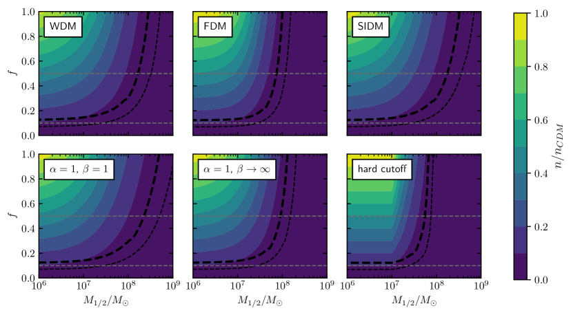
Figure 1: Number of sub-halos $n_{\rm sub}$ in the mass range $10^{7}$–$10^{8}\text{M}_{\odot}$ relative to the CDM prediction $n_{\text{CDM}}$, as a function of the parameters $f$ and $M_{1/2}$ for different models. The parameters for named models are specified in section II. The gray dashed lines show the values between which $f$ is found to be in CDM simulations. The thick and thin black dashed lines show the $68\%$ and $95\%$ CL exclusion limits, respectively, using the analytical likelihood given in ref. Banik et al. (2019a) for the number of halos in the mass bins $10^{7}$–$10^{8}\text{M}_{\odot}$ and $10^{8}$–$10^{9}\text{M}_{\odot}$. We assume that the log-likelihood follows a $\chi^{2}$ distribution with 2 degrees of freedom. A hard cutoff corresponds to a SHMF described by a step function such as below $M_{1/2}$, the number of subhalos is zero.

III Bounds on small-scale clumpiness of the matter distribution and implications for DM phenomenology

Several methods have been proposed and used to place constraints on small-scale DM distribution. Below we give a brief summary of some of the most common techniques.

Stellar dynamics bounds

The presence of dark substructures can be inferred from the dynamical perturbations they induce in their host stellar systems. However, these signals have to be disentangled from the influences of the ‘usual astrophysics’ like globular clusters, molecular clouds, galactic bars, etc. Naturally, the demand for the existence of detailed kinematical data limits the focus here on our own Galaxy.

Several particular probes have been proposed but the full power of this broad direction has still to be realized. For example in Feldmann and Spolyar (2015) the authors estimate that by studying the perturbations in the Galactic disk it should be possible to infer the existence of dark substructures with masses $\sim 10^{8}-10^{9}\,\text{M}_{\odot}$. For masses above $10^{9}\text{M}_{\odot}$, the SHMF is constrained by the abundance of satellite galaxies in the MW Jethwa et al. (2018); Kim et al. (2017); Escudero et al. (2018); Nadler et al. (2019). In Buschmann et al. (2018) a method that searches for characteristic wakes left by the passing substructures in the stellar kinematics of the halo stars is shown to provide sensitivity down to subhalo masses $\sim 10^{7}\,\text{M}_{\odot}$. The main advantage of using halo stars far away from the galactic disk is the reduced contamination from astrophysical backgrounds. However, the hotter the stellar system used for probing substructures, the weaker the bounds one expects to obtain.

The central star cluster in the ultra-faint dwarf galaxy Eridanus II can provide a test for FDM models. In ref. Marsh and Niemeyer (2019) it was argued that this cluster is disrupted by the oscillations of the solitonic core if the FDM particle mass is in the range $10^{-21}$–${10}^{-19}\text{\,}\mathrm{e}\mathrm{V}$. However, it was shown in ref. Schive et al. (2019) that this effect disappears if tidal stripping produced by the MW potential is taken into account.

One of the most promising bounds on dark subhalo population at the moment can be deduced from the detailed observations of surface density fluctuations in stellar streams Ibata et al. (2002); Yoon et al. (2011); Carlberg (2012); Erkal et al. (2016); Bovy et al. (2017); Banik et al. (2018, 2019a); Bonaca et al. (2019) (for a review on stellar streams as probes for the nature of DM see Johnston and Carlberg (2016).) This method might be sensitive to substructure masses as low as $\sim 10^{5}\text{M}_{\odot}$ Yoon et al. (2011); Carlberg (2012); Bovy et al. (2017).

The Milky Way subhalo abundance in the mass ranges $10^{7}$–$10^{8}\text{M}_{\odot}$ and $10^{8}$–$10^{9}\text{M}_{\odot}$ has been estimated from density fluctuations in the density of the cold stellar streams Palomar 5 and GD-1 Banik et al. (2019a). The linear density power spectrum of these streams has been found to be in good agreement with the subhalo abundance predicted by CDM and, thus, in tension with being generated by baryonic structures only.

By fitting the SHMF in eq. (1) to the subhalo abundance in the mass range $10^{7}-10^{9}\text{M}_{\odot}$ given in Banik et al. (2019a), we obtain a rough estimate of the cutoff scale $M_{\text{hm}}$ for different DM scenarios. The predicted number of dark subhalos at a given mass range and DM model can be obtained by integrating the SHMF in eq. (1). By comparing predicted and measured subhalo abundances in the mass range $10^{7}-10^{9}\text{M}_{\odot}$ we set constraints in the plane $(f,M_{1/2})$ for the different DM scenarios discussed in section II and in some idealized toy models (see figure 1). For this purpose, we build a likelihood function which is given by the sum of the analytical probability distribution functions given in Banik et al. (2019a) (cf. equations 6-8) for the subhalo abundance at mass ranges $10^{7}-10^{8}$ and $10^{8}-10^{9}\text{M}_{\odot}$. The resulted log-likelihood is assumed to follow a $\chi^{2}$ with two degrees of freedom. Thus, we compute the 68% and 95% CL exclusion regions which are given by the thick and thin black dashed lines, respectively, in figure 1. We remark that, at higher confidence levels, the suppression of the SHMF can not be constrained using the numerical likelihood given in ref. Banik et al. (2019a) since current observations are not sensible to a low number of subhalos at the given mass range. Moreover, in this case the analytic likelihood fails to approximate the tails of the numerical one.

We find a relatively mild dependence on the shape of the suppression factor specified by parameters $\alpha$ and $\beta$, with the extremal case of a hard cut-off providing the most stringent constraints. In particular, the largest uncertainties are seen to be contained in the survival factor $f$.

Using a log-uniform prior for $f$ in the range $f\in[0.001,0.5]$ the upper bound $M_{\text{hm}}<4.3\times 10^{7}\text{M}_{\odot}$ was reported in ref. Banik et al. (2019a) at 95% CL for the case of a WDM candidate. According to eq. (3), this is equivalent to the 95% CL lower limit $m_{\text{WDM}}>$6.3\text{\,}\mathrm{k}\mathrm{e}\mathrm{V}$$ Banik et al. (2019a). Eq. (7) translates this bound into into the constraint $T_{\text{kd}}>$1.2\text{\,}\mathrm{k}\mathrm{e}\mathrm{V}$$ for the SIDM kinetic decoupling temperature. Similarly, eq. (4) implies a lower bound $m_{\text{FDM}}>$1.9\text{\times}{10}^{-20}\text{\,}\mathrm{e}\mathrm{V}$$ for the mass of the FDM particle. However, since the SHMF depends on the full shape of the power spectrum and on other details of the DM model, it is not possible to make accurate inferences by simply equating the $M_{\text{hm}}$ of different models.

In the range $f=0.1-0.5$, shown by the dashed horizontal lines in figure 1, the 95% CL exclusion boundaries implied for the models under consideration can be summarized as follows:

• WDM:

  $$M_{\text{hm}} <[3.4-43]\times 10^{7}\text{M}_{\odot},$$ (8)

  $$m_{\text{WDM}} >[3.2-6.8]\,$\mathrm{k}\mathrm{e}\mathrm{V}$.$$ (9)

• FDM:

  $$M_{\text{hm}} <[5.4-24]\times 10^{7}\text{M}_{\odot},$$ (10)

  $$m_{\text{FDM}} >[5.2-16]\times 10^{-21}\,$\mathrm{e}\mathrm{V}$.$$ (11)

• SIDM:

  $$M_{\text{cut}} <[1.9-25]\times 10^{7}\text{M}_{\odot},$$ (12)

  $$T_{\text{kd}} >[0.66-1.5]\,$\mathrm{k}\mathrm{e}\mathrm{V}$.$$ (13)

The weaker bounds correspond to $f=0.5$ and the stronger ones to $f=0.1$. The WDM constraint $m_{\text{WDM}}>$6.3\text{\,}\mathrm{k}\mathrm{e}\mathrm{V}$$ in ref. Banik et al. (2019a) corresponds to $f\simeq 0.11$. The SIDM bounds are obtained using the suppression factor in eq. (1) with $\alpha=1$ and $\beta=1.34$. Slightly stronger bounds are found if an exponential suppression factor is used instead.

Stellar kinematical data of MW dwarf galaxies Marsh and Pop (2015); González-Morales et al. (2017); Broadhurst et al. (2019); Wasserman et al. (2019) favors cored DM profiles than can be explained within the FDM scenario for $m_{\text{FDM}}<10^{-21}\,{\rm eV}$. It is important to highlight that the difference between our bound and these limits may reflect systematic errors on the dynamics of dwarf galaxies Oman et al. (2016) rather than a tension in the FDM model. In fact, our lower bound on $m_{\text{FDM}}$ is perfectly compatible with limits set by other experimental strategies, such as Lyman-$\alpha$ Iršič et al. (2017); Kobayashi et al. (2017), CMB Hložek et al. (2018) or X-ray observations Maleki et al. (2020).

Figure 2 shows the bounds on $m_{\text{FDM}}$ obtained from eq. (6). We use $t_{\rm sub}=t_{\rm MW}=13.4\,{\rm Gyr}$ Pasquini et al. (2004) for the age of the subhalos, thus obtaining conservative bounds. We further adopt the linear parametrization of $V(r)(=2\pi r/T_{\rm orb}(r))$ for the Milky Way Eilers et al. (2019):

$$V(r)=$229\text{\,}\mathrm{k}\mathrm{m}\,\mathrm{s}^{-1}$-($1.7\text{\,}\mathrm{k}\mathrm{m}\,\mathrm{s}^{-1}\mathrm{k}\mathrm{p}\mathrm{c}^{-1}$)(r-R_{0}).$$ (14)

where $R_{0}=8.122\pm 0.031\,{\rm kpc}$ is the distance from the Sun to the center of the Galaxy Abuter et al. (2018). The existence of dark subhalos with masses of $10^{7}\,\rm M_{\odot}$ at the perigalacticon of the GD-1 stream $r\simeq$14\text{\,}\mathrm{k}\mathrm{p}\mathrm{c}$$, would then imply a FDM mass satisfying

$$m_{\rm FDM}\gtrsim 10^{-21}\,{\rm eV}.$$ (15)

Constraints inferred using density fluctuations in cold stellar streams might be subject to different sources of systematic error. For instance, it has been recently pointed out that the GD-1 stream, used in the analysis of Banik et al. (2019a), might have been perturbed by the Sagittarius dwarf galaxy Bonaca et al. (2020). Thus, in order to set strong constraints on the DM particle nature, it is important to complement results from different experimental strategies.

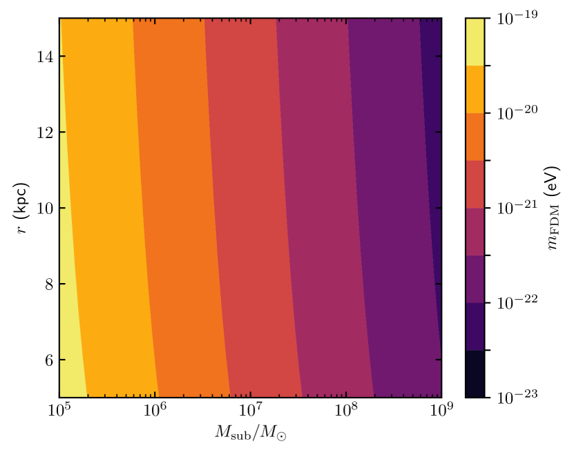
Figure 2: Exclusion boundary for $m_{\text{FDM}}$ assuming subhalos of mass $M_{\rm sub}$ are observed at distance $r$ to the center of the Milky Way, as a function of both $M_{\rm sub}$ and $r$.

Lyman-$\alpha$ bounds

For almost two decades the most stringent and reliable bound on small-scale matter clustering has been obtained via the statistical study of quasar Ly-$\alpha$ forest data, which probes clustering at mildly nonlinear regimes in the redshift interval $z\sim 2-6$, see e.g. Croft et al. (1998, 2002); Seljak et al. (2006); Boyarsky et al. (2009). For instance, the matter power spectrum $P(k)$ at comoving wavenumber $k\simeq 10\,h{\rm Mpc}^{-1}$ cannot be suppressed more than $10\%$ with respect to the standard $\Lambda$CDM case Viel et al. (2013). This has allowed to set a mass limit on thermal relic WDM particle $m_{\rm WDM}>3.3$ keV at $2\sigma$ CL and corresponds to an effective mass-scale suppression in the halo mass function at $\sim 2\times 10^{8}\,h^{-1}\text{M}_{\odot}$ Viel et al. (2013). The above WDM bound translates to the FDM particle mass limit $m_{\rm FDM}\gtrsim 2\times 10^{-21}$ eV, consistent with the mass bounds found in Iršič et al. (2017).

The most recent Ly-$\alpha$ bound is even stronger, ruling out WDM masses below $10$ keV at $95\%$ CL. Palanque-Delabrouille et al. (2019). Using eqs. (3), (7) and (4), this bound roughly translates into $T_{\text{kd}}>$2.0\text{\,}\mathrm{k}\mathrm{e}\mathrm{V}$$ and $m_{\text{FDM}}>$5.9\text{\times}{10}^{-20}\text{\,}\mathrm{e}\mathrm{V}$$. However, considering realistic astrophysical uncertainties on the modeling of the intergalactic medium, this result is highly controversial Garzilli et al. (2019).

SIDM scenarios have been considered in the context of Ly-$\alpha$ observations in ref. Archidiacono et al. (2019) and Ly-$\alpha$ constraints on the PBH abundance have been derived in Murgia et al. (2019).

Lensing bounds

More recently a direct detection of substructures in high resolution imaging data of giant strong lensing arcs has become a new competitive method, currently enabling to detect subhaloes with masses down to $\sim 10^{8}-10^{9}\,\text{M}_{\odot}$. For example in Vegetti et al. (2010) a Hubble Space Telescope imaging has been used to detect substructure with mass $\sim 3.5\times 10^{9}\,\text{M}_{\odot}$ in a lens galaxy at redshift $z\sim 0.22$ having total DM mass $\sim 3.6\times 10^{11}\,\text{M}_{\odot}$ inside the effective radius. In Vegetti et al. (2012) Keck adaptive optics imaging has revealed a substructure with mass $\sim 1.9\times 10^{8}\,\text{M}_{\odot}$ in a Sagittarius-size lens galaxy at redshift $z\sim 0.88$. In Hezaveh et al. (2016b) a subclump with mass $\sim 9\times 10^{8}\,\text{M}_{\odot}$ has been detected using ALMA observations of the strong lensing system SDP.81.

Instead of the above direct subclump detection these techniques can be extended via statistical fluctuation analyses to probe the presence of substructures below a direct detection limit, potentially allowing to reach down to masses $\sim 10^{7}\,\text{M}_{\odot}$, see e.g. Hezaveh et al. (2016a); Díaz Rivero et al. (2018); Brehmer et al. (2019).

Yet another approach to constrain substructures relies on measurements of flux ratios of strongly lensed quasars, which allows to indirectly probe the presence of subclumps with masses $\sim 10^{6}-10^{9}\,\text{M}_{\odot}$ Hsueh et al. (2019). This has allowed to constrain the thermal relic WDM particle mass $m_{\rm WDM}>3.8$ keV at $2\sigma$ CL Hsueh et al. (2019), i.e., comparable to the level of the above Ly-$\alpha$ bounds. Since these constraints rely on the non-linear substructure, they cannot be straightforwardly mapped to bounds on other DM models via $M_{\text{hm}}$ comparisons.

IV Prospects

A subhalo interaction with a tidal stream perturbs the energy distribution for the member stars of the latter. This perturbation in orbital energy evolves into fluctuations in surface density at different angular scales depending on the mass and velocity of the perturber, the impact parameter and look-back time at which the interaction took place Yoon et al. (2011); Carlberg (2012). Therefore, the population of subhalos orbiting a galaxy can be characterized using measurements of the surface density of stellar streams. Up to know, this analysis has been reduced to the Pal 5 and GD-1 stellar streams (see e.g. Carlberg (2012); Bonaca et al. (2018); Banik et al. (2019a)).

The number of known stellar streams has significantly increased in the past 5 years due to the advent of large sky photometric and astrometric surveys, such as the Sloan Digital Sky Survey, Dark Energy Survey, Pan-STARRS1 and Gaia. A compilation of known stellar streams can be found in the galstream python package Mateu et al. (2018). However, only for roughly 10% of these streams - for those that have been spectroscopically followed up - properties about their orbits and progenitors can be inferred. The near-future spectroscopic facilities (such as, 4MOST or DESI), are expected to increase, on the one hand, the number of cold tidal streams with known orbit and kinematics and, on the other hand, the number of member stars of individual streams, thus reducing measurement errors on the surface density. These improvements might lead to a sensitivity to the effects of subhalos with masses as low as $10^{5}\,\rm M_{\odot}$ Yoon et al. (2011); Carlberg (2012); Bovy et al. (2017). To fully take advantage of the potential of stellar stream observations, experimental advances need to be accompanied by improvements on the theoretical modeling of streams Bonaca et al. (2020); Morinaga et al. (2019).

The most stringent bound that could be imposed in this case is thus $M_{\text{hm}}\lesssim 10^{5}\text{M}_{\odot}$ and therefore WDM, SIDM and FDM scenarios with parameter values up to

$$m_{\text{WDM}} \sim$40\text{\,}\mathrm{k}\mathrm{e}\mathrm{V}$,$$ (16)

$$T_{\text{kd}} \sim$9\text{\,}\mathrm{k}\mathrm{e}\mathrm{V}$,$$

$$m_{\text{FDM}} \sim$2\text{\times}{10}^{-18}\text{\,}\mathrm{e}\mathrm{V}$,$$

may be probed. Since FDM models could alleviate small-scale discrepancies when $m_{\rm FDM}\lesssim${10}^{-21}\text{\,}\mathrm{e}\mathrm{V}$$, realizing the full potential of from stellar stream observations can certainly test the FDM explanation of the small-scale problems. A similar conclusion can be drawn for WDM and SIDM models, especially when the resolution of the small scale discrepancies rests on the early suppression of the linear power spectrum.

V Discussion and conclusions

In this paper we considered different DM scenarios in the light of the recent indirectly measurement of dark subhalo abundance from the stellar density fluctuations of tidal streams. Stellar streams provide a promising set of observables for constraining small-scale structure and thus, studying the DM particle nature owing to the differences in subhalo abundances predicted by different DM models. As shown in section III, current stellar stream limits are already at the level of the ones obtained from other observables, such as Lyman-$\alpha$ or gravitational lensing. In the conservative case, for WDM we obtain the lower bound $m_{\text{WDM}}>$3.2\text{\,}\mathrm{k}\mathrm{e}\mathrm{V}$$ which is slightly lower that found Banik et al. (2019a). Similarly, we find that the FDM mass must satisfy $m_{\text{FDM}}>$5.2\text{\times}{10}^{-21}\text{\,}\mathrm{e}\mathrm{V}$$ and for SIDM scenarios where DM is coupled to a dark radiation bath, kinetic decoupling must take place at temperatures higher than $T_{\text{kd}}>$0.7\text{\,}\mathrm{k}\mathrm{e}\mathrm{V}$$.

A significant improvement on these bounds can be expected in the near future with the advent of large sky photometric and spectroscopic surveys which will increase the number of known streams and the number of member stars belonging to a given stellar stream. In order to fully realize the potential of these measurements, it would be necessary to improve our understanding of baryonic effects in disrupting DM subhalos. Also, an improved theoretical understanding of the substructure in SIDM models is required in order to effectively study them using stellar dynamics measurements.

Tidal stripping and disruption of subhalos due to baryonic effects is difficult to quantify. Modifications in the SHMF induced by these effects depend on the density profile of the subhalos, with cored profiles more prone to disruption Errani and Peñarrubia (2019). The latter itself is dependent on the underlying DM physics. In our simplified framework we parametrize our lack of knowledge through the survival fraction $f$ that can take values in a relatively wide range (see e.g. D’Onghia et al. (2010); Sawala et al. (2017); Garrison-Kimmel et al. (2017)). The most conservative bounds for the modified DM scenarios can be obtained by choosing $f=1$. In order to distinguish different DM scenarios, on the other hand, an accurate estimate of the baryonic effects on the suppression of the subhalo abundance is required. Moreover, if the nature of DM would be determined from other observables, then stellar stream observations may help to precisely determine the baryonic effects i.e., the value of $f$ in our simplified framework.

At any rate, since the different methods that aim to determine the number of subhalos are affected by different sources of systematic error, it is the complementarity of them that would allow to set robust constraints on the particle nature of DM.

The population of dark subhalos in our Galaxy further affects indirect DM searches which aim at detecting the flux of final stable particles produced by annihilation or decay of Weakly Interacting Massive Particles. The flux of stable particles depends on the distribution of DM in the region under study and the presence of subhalos can significantly boost this signal Moliné et al. (2017). The subhalo abundance also impacts searches for annihilation signals from optically faint patches of the sky Calore et al. (2019).

Note added: During completion of this work a related study on FDM Schutz (2020) appeared, where similar conclusions regarding FDM are reached using a slightly different modification of the SHMF (see also appendix A).

Appendix A Analytic fitting forms for WDM & FDM

In the following we assume analytic description for the SHMF as presented in Schneider (2015), where it has been extensively tested against WDM and mixedDM (warm+cold) N-body simulations with a wide range of effective small-scale power suppression scales. Even though a precise treatment for the FDM would require numerical integration of the Scrödinger-Poisson system in place of the usual Vlasov-Poisson system of the collisionless N-body problem, the above analytic model should still serve as a reasonably good approximation. The linear input spectra for the SHMF calculations were calculated with CAMBLewis et al. (2000) and axionCAMBHlozek et al. (2015) Boltzmann codes (for WDM and FDM, respectively). Spatially flat cosmologies with $\Omega_{m}=0.3$, $\Omega_{\rm WDM/FDM}=0.25$, $h=0.7$ were assumed.

It turns out that the results of our analytical calculations can be quite well approximated by the following functional form

$$\frac{dn_{\rm sub}}{dM} =R(M;\alpha,\beta,\gamma)\left(\frac{dn_{\rm sub}}{dM}\right)_{\text{CDM}}$$ (17)

$$R(M;\alpha,\beta,\gamma) \equiv\left[1+\left(\frac{\gamma M_{\text{hm}}}{M}\right)^{\alpha}\right]^{-\beta}\,,$$

with best-fit parameters

• WDM: $\alpha\simeq 0.76$, $\beta\simeq 3.9$, $\gamma\simeq 0.087$,

• FDM: $\alpha\simeq 1.5$, $\beta\simeq 5.0$, $\gamma\simeq 0.14$ .

The above WDM fit is fine for $m_{\rm WDM}\sim 4-8$ keV but it can be significantly improved for lower and higher masses by allowing $\beta$ to vary with $m_{\rm WDM}$

$$\beta \simeq 3.14-0.057\times m_{\rm WDM}[{\rm keV}]\,,$$

$$\alpha \simeq 0.785\,,$$

$$\gamma \simeq 0.153\,.$$

Here the half-mode mass $M_{\text{hm}}$ is given by eq. (2) where $M_{\text{hm}}$ for WDM is shown in eq. (3) while for FDM we use the following slightly improved fit over the one provided in Hu et al. (2000):

$$M_{\text{hm}}\simeq 6.3\times 10^{10}\,{\rm M_{\odot}}\left(\frac{\Omega_{m}}{0.3}\right)\left(\frac{h}{0.7}\right)^{2}\left(\frac{m_{\text{FDM}}}{${10}^{-22}\text{\,}\mathrm{e}\mathrm{V}$}\right)^{-1.38}.$$ (18)

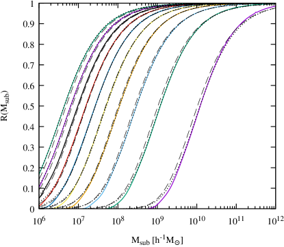
Figure 3: Ratio of WDM and CDM SHMFs. The WDM particle mass is in range $1-10$ keV with $1$ keV step size. Fitting functions (17) with constant and mass-varying $\beta$ are shown with dashed and dotted lines, respectively.

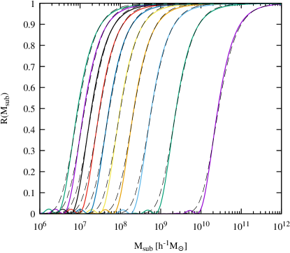
Figure 4: Ratio of FDM and CDM SHMFs. Here the FDM particle masses are obtained from the WDM masses of figure 3 via the approximate relation (19) and cover a range $\sim(1-300)\times 10^{-22}$ eV. Fitting function (17) is shown with dashed lines.

The performance of the fitting form (17) against direct analytic calculations is shown in figures 3 and 4 for WDM and FDM, respectively. Here the solid lines correspond to direct analytic calculations and dashed ones show the approximation form (17). In figure 3, starting from the line with the strongest suppression, the WDM mass increases from $m_{\rm WDM}=1$ keV up to $10$ keV with $1$ keV step size. The FDM masses in figure 4 correspond to the WDM particle masses of figure 3 by requiring the linear power suppression wavenumbers $k_{\text{hm}}$ to approximately match. In particular, this amounts to choosing

$$m_{\rm FDM}\sim\left(\frac{m_{\rm WDM}}{{\rm keV}}\right)^{2.5}\times 10^{-22}\,{\rm eV}\,.$$ (19)

In a recent paper Schutz (2020), which studied topics similar to the ones covered in this work, the author used an analytic FDM substructure fitting function obtained earlier in Du (2018). It turns out that our FDM results shown in figure 4 have somewhat stronger suppression. The results can be made to agree roughly if we increase $m_{\rm FDM}$ by a factor $\sim 4-5$. One possibility for this discrepancy could be the form of the filtering function used in calculations: Fourier vs real-space top-hat function. In Schneider (2015), in context of WDM models, it was extensively discussed that standard Press-Schechter calculations with real-space top-hat function leads to a significant underestimation of the small-scale substructure suppression factor when compared with direct N-body results. However, it turns out that this is not the case here, since the fitting functions of Du (2018) also assumed sharp Fourier-space filter. Further studies are needed to resolve this discrepancy. For a possible explanation see the updated version of Schutz (2020). In general, one needs dedicated high resolution numerical simulations to reliably calibrate the analytic SHMF. Unfortunately, currently available simulations lack resolution to reach conclusive results.

Appendix B Comparison with arXiv:2003.01125

During the reviewing process of this paper a simulation work Lovell (2020) appeared, which gave the results for the WDM SHMFs using identical fitting form to the one adopted here, cf., (17). It is instructive to see how our results compare. At first sight, the best-fit parameter values obtained there

$$\alpha\simeq 2.5,\,\beta\simeq 0.2,\,\gamma\simeq 4.2$$

seem to differ remarkably from ours:

$$\alpha\simeq 0.76,\,\beta\simeq 3.9,\,\gamma\simeq 0.087h^{-1}\simeq 0.12\,.$$

Note that we have adjusted our $\gamma$ parameter to count for the fact that in Lovell (2020) mass was measured in plain Solar masses, rather than in $h^{-1}\text{M}_{\odot}$, as is assumed throughout this work.

Here we want to show that for substructure suppression factors $R\sim 0.3-0.7$ both fits agree remarkably well. To see this let us re-express Eq. (17)

$$R(M)=\left[1+(2^{1/\beta}-1)\left(\frac{M_{\nicefrac{{1}}{{2}}}}{M}\right)^{\alpha}\right]^{-\beta}\,,$$ (20)

where $M_{\nicefrac{{1}}{{2}}}$ is defined via $R(M_{\nicefrac{{1}}{{2}}})\equiv\nicefrac{{1}}{{2}}$. It is related to $M_{\text{hm}}$ as

$$M_{\nicefrac{{1}}{{2}}}=\frac{\gamma}{(2^{1/\beta}-1)^{1/\alpha}}M_{\text{hm}}\,.$$ (21)

Around masses $M_{\nicefrac{{1}}{{2}}}$ the substructure suppression factor $R(M)$ is well approximated by a linear relation in $R(M)$-$\ln(M)$ axes

$$R(M) \simeq\frac{1}{2}+n\cdot\ln\left(\frac{M}{M_{\nicefrac{{1}}{{2}}}}\right)\,,$$ (22)

$$n \equiv\frac{1}{2}\alpha\beta\left(1-2^{-1/\beta}\right)\,.$$

It is easy to check that both sets of $\alpha$, $\beta$ and $\gamma$ parameters, as presented above, give practically the same values for $n$ and $M_{\nicefrac{{1}}{{2}}}$:

• our best-fit parameters result in:
  $M_{\nicefrac{{1}}{{2}}}\simeq 1.03M_{\text{hm}}$, $n\simeq 0.24$ ,

• whereas parameters of Lovell (2020) give:
  $M_{\nicefrac{{1}}{{2}}}\simeq 1.06M_{\text{hm}}$, $n\simeq 0.24$ .

Thus, around $M_{\nicefrac{{1}}{{2}}}$ both fits are practically identical. This is illustrated in Figure 5.

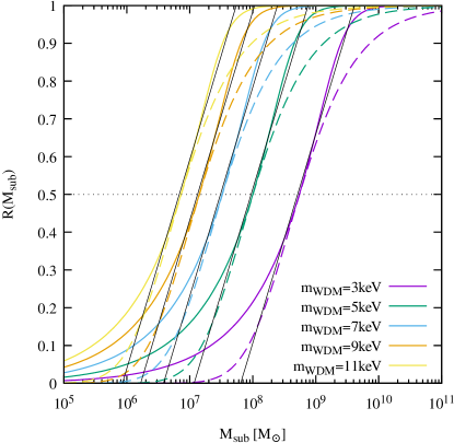
Figure 5: Comparison of substructure suppression factors. Solid and long-dashed lines present fits obtained in Lovell (2020) and in this work, respectively. $M_{\text{hm}}$ corresponds to $m_{\text{WDM}}$ values as given in the legend. Thin black lines display approximating function Eq. (22) (with $M_{\nicefrac{{1}}{{2}}}=M_{\text{hm}}$).

It is quite remarkable that the WDM fitting formulas of the current work, which are based on the analytic formalism of Schneider (2015), agree so well with the N-body results of Lovell (2020) down to substructure suppression factors of $R\sim 1/2$ and below. One also has to bear in mind that the values for the best-fit $\alpha$, $\beta$ and $\gamma$ parameters obtained in this work were largely driven by the behaviour of the function $R(M)$ at large values of $M$, which are hard to probe in limited set of N-body simulations. Additionally, at small masses simulations have lots of small-scale clumps out of which a significant fraction might be spurious systems.

References

- Jungman et al. (1996) G. Jungman, M. Kamionkowski, and K. Griest, Phys.Rept. 267, 195 (1996), arXiv:hep-ph/9506380 .
- Bertone et al. (2005) G. Bertone, D. Hooper, and J. Silk, Phys.Rept. 405, 279 (2005), arXiv:hep-ph/0404175 .
- Klypin et al. (1999) A. A. Klypin, A. V. Kravtsov, O. Valenzuela, and F. Prada, Astrophys. J. 522, 82 (1999), arXiv:astro-ph/9901240 [astro-ph] .
- Moore et al. (1999a) B. Moore, S. Ghigna, F. Governato, G. Lake, T. R. Quinn, J. Stadel, and P. Tozzi, Astrophys. J. 524, L19 (1999a), arXiv:astro-ph/9907411 [astro-ph] .
- Boylan-Kolchin et al. (2011) M. Boylan-Kolchin, J. S. Bullock, and M. Kaplinghat, Mon. Not. Roy. Astron. Soc. 415, L40 (2011), arXiv:1103.0007 [astro-ph.CO] .
- Boylan-Kolchin et al. (2012) M. Boylan-Kolchin, J. S. Bullock, and M. Kaplinghat, Mon. Not. Roy. Astron. Soc. 422, 1203 (2012), arXiv:1111.2048 [astro-ph.CO] .
- Garrison-Kimmel et al. (2014) S. Garrison-Kimmel, M. Boylan-Kolchin, J. S. Bullock, and E. N. Kirby, Mon. Not. Roy. Astron. Soc. 444, 222 (2014), arXiv:1404.5313 [astro-ph.GA] .
- Papastergis et al. (2015) E. Papastergis, R. Giovanelli, M. P. Haynes, and F. Shankar, Astron. Astrophys. 574, A113 (2015), arXiv:1407.4665 [astro-ph.GA] .
- Kaplinghat et al. (2019) M. Kaplinghat, M. Valli, and H.-B. Yu, Mon. Not. Roy. Astron. Soc. 490, 231 (2019), arXiv:1904.04939 [astro-ph.GA] .
- Moore (1994) B. Moore, Nature 370, 629 (1994).
- Flores and Primack (1994) R. A. Flores and J. R. Primack, Astrophys. J. 427, L1 (1994), arXiv:astro-ph/9402004 [astro-ph] .
- Burkert (1996) A. Burkert, IAU Symposium 171: New Light on Galaxy Evolution Heidelberg, Germany, June 26-30, 1995, IAU Symp. 171, 175 (1996), [Astrophys. J.447,L25(1995)], arXiv:astro-ph/9504041 [astro-ph] .
- Moore et al. (1999b) B. Moore, T. R. Quinn, F. Governato, J. Stadel, and G. Lake, Mon. Not. Roy. Astron. Soc. 310, 1147 (1999b), arXiv:astro-ph/9903164 [astro-ph] .
- van den Bosch and Swaters (2001) F. C. van den Bosch and R. A. Swaters, Mon. Not. Roy. Astron. Soc. 325, 1017 (2001), arXiv:astro-ph/0006048 [astro-ph] .
- de Blok et al. (2001) W. J. G. de Blok, S. S. McGaugh, A. Bosma, and V. C. Rubin, Astrophys. J. 552, L23 (2001), arXiv:astro-ph/0103102 [astro-ph] .
- Pawlowski et al. (2013) M. S. Pawlowski, P. Kroupa, and H. Jerjen, Mon. Not. Roy. Astron. Soc. 435, 1928 (2013), arXiv:1307.6210 [astro-ph.CO] .
- Oman et al. (2015) K. A. Oman et al., Mon. Not. Roy. Astron. Soc. 452, 3650 (2015), arXiv:1504.01437 [astro-ph.GA] .
- Kuhlen et al. (2012) M. Kuhlen, M. Vogelsberger, and R. Angulo, Phys. Dark Univ. 1, 50 (2012), arXiv:1209.5745 [astro-ph.CO] .
- Tulin and Yu (2018) S. Tulin and H.-B. Yu, Phys. Rept. 730, 1 (2018), arXiv:1705.02358 [hep-ph] .
- Bullock and Boylan-Kolchin (2017) J. S. Bullock and M. Boylan-Kolchin, ARA&A 55, 343 (2017), arXiv:1707.04256 [astro-ph.CO] .
- Bode et al. (2001) P. Bode, J. P. Ostriker, and N. Turok, Astrophys.J. 556, 93 (2001), arXiv:astro-ph/0010389 .
- Colin et al. (2000) P. Colin, V. Avila-Reese, and O. Valenzuela, Astrophys. J. 542, 622 (2000), arXiv:astro-ph/0004115 [astro-ph] .
- Hu et al. (2000) W. Hu, R. Barkana, and A. Gruzinov, Phys. Rev. Lett. 85, 1158 (2000), arXiv:astro-ph/0003365 [astro-ph] .
- Schive et al. (2016) H.-Y. Schive, T. Chiueh, T. Broadhurst, and K.-W. Huang, Astrophys. J. 818, 89 (2016), arXiv:1508.04621 [astro-ph.GA] .
- Marsh (2016a) D. J. E. Marsh, Phys. Rept. 643, 1 (2016a), arXiv:1510.07633 [astro-ph.CO] .
- Hui et al. (2017) L. Hui, J. P. Ostriker, S. Tremaine, and E. Witten, Phys. Rev. D95, 043541 (2017), arXiv:1610.08297 [astro-ph.CO] .
- Du et al. (2017) X. Du, C. Behrens, and J. C. Niemeyer, Mon. Not. Roy. Astron. Soc. 465, 941 (2017), arXiv:1608.02575 [astro-ph.CO] .
- Cyr-Racine and Sigurdson (2013) F.-Y. Cyr-Racine and K. Sigurdson, Phys. Rev. D87, 103515 (2013), arXiv:1209.5752 [astro-ph.CO] .
- Vogelsberger et al. (2012) M. Vogelsberger, J. Zavala, and A. Loeb, Mon. Not. Roy. Astron. Soc. 423, 3740 (2012), arXiv:1201.5892 [astro-ph.CO] .
- Vogelsberger et al. (2016) M. Vogelsberger, J. Zavala, F.-Y. Cyr-Racine, C. Pfrommer, T. Bringmann, and K. Sigurdson, Mon. Not. Roy. Astron. Soc. 460, 1399 (2016), arXiv:1512.05349 [astro-ph.CO] .
- Huo et al. (2018) R. Huo, M. Kaplinghat, Z. Pan, and H.-B. Yu, Phys. Lett. B783, 76 (2018), arXiv:1709.09717 [hep-ph] .
- Hawking (1971) S. Hawking, Mon. Not. Roy. Astron. Soc. 152, 75 (1971).
- Carr and Hawking (1974) B. J. Carr and S. W. Hawking, Mon. Not. Roy. Astron. Soc. 168, 399 (1974).
- Carr et al. (2016) B. Carr, F. Kuhnel, and M. Sandstad, Phys. Rev. D94, 083504 (2016), arXiv:1607.06077 [astro-ph.CO] .
- Murgia et al. (2019) R. Murgia, G. Scelfo, M. Viel, and A. Raccanelli, Phys. Rev. Lett. 123, 071102 (2019), arXiv:1903.10509 [astro-ph.CO] .
- Hütsi et al. (2019) G. Hütsi, M. Raidal, and H. Veermäe, Phys. Rev. D100, 083016 (2019), arXiv:1907.06533 [astro-ph.CO] .
- Inman and Ali-Haïmoud (2019) D. Inman and Y. Ali-Haïmoud, Phys. Rev. D100, 083528 (2019), arXiv:1907.08129 [astro-ph.CO] .
- Vegetti et al. (2010) S. Vegetti, L. V. E. Koopmans, A. Bolton, T. Treu, and R. Gavazzi, Mon. Not. Roy. Astron. Soc. 408, 1969 (2010), arXiv:0910.0760 [astro-ph.CO] .
- Vegetti et al. (2012) S. Vegetti, D. J. Lagattuta, J. P. McKean, M. W. Auger, C. D. Fassnacht, and L. V. E. Koopmans, Nature 481, 341 (2012), arXiv:1201.3643 [astro-ph.CO] .
- Hezaveh et al. (2016a) Y. Hezaveh, N. Dalal, G. Holder, T. Kisner, M. Kuhlen, and L. Perreault Levasseur, JCAP 1611, 048 (2016a), arXiv:1403.2720 [astro-ph.CO] .
- Hezaveh et al. (2016b) Y. D. Hezaveh et al., Astrophys. J. 823, 37 (2016b), arXiv:1601.01388 [astro-ph.CO] .
- Díaz Rivero et al. (2018) A. Díaz Rivero, C. Dvorkin, F.-Y. Cyr-Racine, J. Zavala, and M. Vogelsberger, Phys. Rev. D 98, 103517 (2018), arXiv:1809.00004 [astro-ph.CO] .
- Brehmer et al. (2019) J. Brehmer, S. Mishra-Sharma, J. Hermans, G. Louppe, and K. Cranmer, arXiv e-prints , arXiv:1909.02005 (2019), arXiv:1909.02005 [astro-ph.CO] .
- Hsueh et al. (2019) J.-W. Hsueh, W. Enzi, S. Vegetti, M. Auger, C. D. Fassnacht, G. Despali, L. V. E. Koopmans, and J. P. McKean, (2019), arXiv:1905.04182 [astro-ph.CO] .
- Alexander et al. (2019a) S. Alexander, S. Gleyzer, E. McDonough, M. W. Toomey, and E. Usai, (2019a), arXiv:1909.07346 [astro-ph.CO] .
- Gilman et al. (2020) D. Gilman, S. Birrer, A. Nierenberg, T. Treu, X. Du, and A. Benson, MNRAS 491, 6077 (2020), arXiv:1908.06983 [astro-ph.CO] .
- Croft et al. (1998) R. A. C. Croft, D. H. Weinberg, N. Katz, and L. Hernquist, Astrophys. J. 495, 44 (1998), arXiv:astro-ph/9708018 [astro-ph] .
- Croft et al. (2002) R. A. C. Croft, D. H. Weinberg, M. Bolte, S. Burles, L. Hernquist, N. Katz, D. Kirkman, and D. Tytler, Astrophys. J. 581, 20 (2002), arXiv:astro-ph/0012324 [astro-ph] .
- Viel et al. (2013) M. Viel, G. D. Becker, J. S. Bolton, and M. G. Haehnelt, Phys. Rev. D88, 043502 (2013), arXiv:1306.2314 [astro-ph.CO] .
- Seljak et al. (2006) U. Seljak, A. Slosar, and P. McDonald, JCAP 0610, 014 (2006), arXiv:astro-ph/0604335 [astro-ph] .
- Boyarsky et al. (2009) A. Boyarsky, J. Lesgourgues, O. Ruchayskiy, and M. Viel, J. Cosmology Astropart. Phys 2009, 012 (2009), arXiv:0812.0010 [astro-ph] .
- Iršič et al. (2017) V. Iršič, M. Viel, M. G. Haehnelt, J. S. Bolton, and G. D. Becker, Phys. Rev. Lett. 119, 031302 (2017), arXiv:1703.04683 [astro-ph.CO] .
- Palanque-Delabrouille et al. (2019) N. Palanque-Delabrouille, C. Yèche, N. Schöneberg, J. Lesgourgues, M. Walther, S. Chabanier, and E. Armengaud, arXiv e-prints , arXiv:1911.09073 (2019), arXiv:1911.09073 [astro-ph.CO] .
- Ibata et al. (2002) R. A. Ibata, G. F. Lewis, M. J. Irwin, and T. Quinn, MNRAS 332, 915 (2002), arXiv:astro-ph/0110690 [astro-ph] .
- Yoon et al. (2011) J. H. Yoon, K. V. Johnston, and D. W. Hogg, ApJ 731, 58 (2011), arXiv:1012.2884 [astro-ph.GA] .
- Carlberg (2012) R. G. Carlberg, ApJ 748, 20 (2012), arXiv:1109.6022 [astro-ph.CO] .
- Feldmann and Spolyar (2015) R. Feldmann and D. Spolyar, Mon. Not. Roy. Astron. Soc. 446, 1000 (2015), arXiv:1310.2243 [astro-ph.GA] .
- Bovy et al. (2017) J. Bovy, D. Erkal, and J. L. Sanders, Mon. Not. Roy. Astron. Soc. 466, 628 (2017), arXiv:1606.03470 [astro-ph.GA] .
- Erkal et al. (2016) D. Erkal, V. Belokurov, J. Bovy, and J. L. Sand ers, MNRAS 463, 102 (2016), arXiv:1606.04946 [astro-ph.GA] .
- Buschmann et al. (2018) M. Buschmann, J. Kopp, B. R. Safdi, and C.-L. Wu, Phys. Rev. Lett. 120, 211101 (2018), arXiv:1711.03554 [astro-ph.GA] .
- Kim et al. (2017) S. Y. Kim, A. H. G. Peter, and J. R. Hargis, arXiv e-prints , arXiv:1711.06267 (2017), arXiv:1711.06267 [astro-ph.CO] .
- Escudero et al. (2018) M. Escudero, L. Lopez-Honorez, O. Mena, S. Palomares-Ruiz, and P. Villanueva-Domingo, J. Cosmology Astropart. Phys 2018, 007 (2018), arXiv:1803.08427 [astro-ph.CO] .
- Jethwa et al. (2018) P. Jethwa, D. Erkal, and V. Belokurov, MNRAS 473, 2060 (2018), arXiv:1612.07834 [astro-ph.GA] .
- Marsh and Niemeyer (2019) D. J. E. Marsh and J. C. Niemeyer, Phys. Rev. Lett. 123, 051103 (2019), arXiv:1810.08543 [astro-ph.CO] .
- Banik et al. (2018) N. Banik, G. Bertone, J. Bovy, and N. Bozorgnia, JCAP 1807, 061 (2018), arXiv:1804.04384 [astro-ph.CO] .
- Schive et al. (2019) H.-Y. Schive, T. Chiueh, and T. Broadhurst, (2019), arXiv:1912.09483 [astro-ph.GA] .
- Nadler et al. (2019) E. O. Nadler, V. Gluscevic, K. K. Boddy, and R. H. Wechsler, ApJ 878, L32 (2019), arXiv:1904.10000 [astro-ph.CO] .
- Bonaca et al. (2019) A. Bonaca, D. W. Hogg, A. M. Price-Whelan, and C. Conroy, ApJ 880, 38 (2019), arXiv:1811.03631 [astro-ph.GA] .
- Banik et al. (2019a) N. Banik, J. Bovy, G. Bertone, D. Erkal, and T. J. L. de Boer, (2019a), arXiv:1911.02662 [astro-ph.GA] .
- Banik et al. (2019b) N. Banik, J. Bovy, G. Bertone, D. Erkal, and T. J. L. de Boer, (2019b), arXiv:1911.02663 [astro-ph.GA] .
- Schneider et al. (2012) A. Schneider, R. E. Smith, A. V. Macciò, and B. Moore, MNRAS 424, 684 (2012), arXiv:1112.0330 [astro-ph.CO] .
- D’Onghia et al. (2010) E. D’Onghia, V. Springel, L. Hernquist, and D. Keres, ApJ 709, 1138 (2010), arXiv:0907.3482 [astro-ph.CO] .
- Sawala et al. (2017) T. Sawala, P. Pihajoki, P. H. Johansson, C. S. Frenk, J. F. Navarro, K. A. Oman, and S. D. M. White, MNRAS 467, 4383 (2017), arXiv:1609.01718 [astro-ph.GA] .
- Garrison-Kimmel et al. (2017) S. Garrison-Kimmel, A. Wetzel, J. S. Bullock, P. F. Hopkins, M. Boylan-Kolchin, C.-A. Faucher-Giguère, D. Kereš, E. Quataert, R. E. Sanderson, A. S. Graus, and T. Kelley, MNRAS 471, 1709 (2017), arXiv:1701.03792 [astro-ph.GA] .
- Errani and Peñarrubia (2019) R. Errani and J. Peñarrubia, arXiv e-prints , arXiv:1906.01642 (2019), arXiv:1906.01642 [astro-ph.GA] .
- Lovell et al. (2014) M. R. Lovell, C. S. Frenk, V. R. Eke, A. Jenkins, L. Gao, and T. Theuns, Mon.Not.Roy.Astron.Soc. 439, 300 (2014), arXiv:1308.1399 [astro-ph.CO] .
- Schneider (2015) A. Schneider, Mon. Not. Roy. Astron. Soc. 451, 3117 (2015), arXiv:1412.2133 [astro-ph.CO] .
- Viel et al. (2005) M. Viel, J. Lesgourgues, M. G. Haehnelt, S. Matarrese, and A. Riotto, Phys. Rev. D 71, 063534 (2005), arXiv:astro-ph/0501562 [astro-ph] .
- Marsh (2016b) D. J. E. Marsh, (2016b), arXiv:1605.05973 [astro-ph.CO] .
- Du et al. (2018) X. Du, B. Schwabe, J. C. Niemeyer, and D. Bürger, Phys. Rev. D97, 063507 (2018), arXiv:1801.04864 [astro-ph.GA] .
- Alexander et al. (2019b) S. Alexander, J. J. Bramburger, and E. McDonough, Phys. Lett. B797, 134871 (2019b), arXiv:1901.03694 [astro-ph.CO] .
- Boehm et al. (2002) C. Boehm, A. Riazuelo, S. H. Hansen, and R. Schaeffer, Phys. Rev. D66, 083505 (2002), arXiv:astro-ph/0112522 [astro-ph] .
- Buckley et al. (2014) M. R. Buckley, J. Zavala, F.-Y. Cyr-Racine, K. Sigurdson, and M. Vogelsberger, Phys. Rev. D90, 043524 (2014), arXiv:1405.2075 [astro-ph.CO] .
- Boehm et al. (2014) C. Boehm, J. A. Schewtschenko, R. J. Wilkinson, C. M. Baugh, and S. Pascoli, Mon. Not. Roy. Astron. Soc. 445, L31 (2014), arXiv:1404.7012 [astro-ph.CO] .
- Vogelsberger et al. (2014) M. Vogelsberger, J. Zavala, C. Simpson, and A. Jenkins, Mon. Not. Roy. Astron. Soc. 444, 3684 (2014), arXiv:1405.5216 [astro-ph.CO] .
- Kaplan et al. (2010) D. E. Kaplan, G. Z. Krnjaic, K. R. Rehermann, and C. M. Wells, JCAP 1005, 021 (2010), arXiv:0909.0753 [hep-ph] .
- Johnston and Carlberg (2016) K. V. Johnston and R. G. Carlberg, “Tidal Debris as a Dark Matter Probe,” in Tidal Streams in the Local Group and Beyond, Astrophysics and Space Science Library, Volume 420. ISBN 978-3-319-19335-9. Springer International Publishing Switzerland, 2016, p. 169, Astrophysics and Space Science Library, Vol. 420, edited by H. J. Newberg and J. L. Carlin (2016) p. 169.
- Marsh and Pop (2015) D. J. E. Marsh and A.-R. Pop, MNRAS 451, 2479 (2015), arXiv:1502.03456 [astro-ph.CO] .
- González-Morales et al. (2017) A. X. González-Morales, D. J. E. Marsh, J. Peñarrubia, and L. A. Ureña-López, MNRAS 472, 1346 (2017), arXiv:1609.05856 [astro-ph.CO] .
- Broadhurst et al. (2019) T. Broadhurst, I. de Martino, H. Nhan Luu, G. F. Smoot, and S. H. H. Tye, arXiv e-prints , arXiv:1902.10488 (2019), arXiv:1902.10488 [astro-ph.CO] .
- Wasserman et al. (2019) A. Wasserman, P. van Dokkum, A. J. Romanowsky, J. Brodie, S. Danieli, D. A. Forbes, R. Abraham, C. Martin, M. Matuszewski, A. Villaume, J. Tamanas, and S. Profumo, ApJ 885, 155 (2019), arXiv:1905.10373 [astro-ph.GA] .
- Oman et al. (2016) K. A. Oman, J. F. Navarro, L. V. Sales, A. Fattahi, C. S. Frenk, T. Sawala, M. Schaller, and S. D. M. White, MNRAS 460, 3610 (2016), arXiv:1601.01026 [astro-ph.GA] .
- Iršič et al. (2017) V. Iršič, M. Viel, M. G. Haehnelt, J. S. Bolton, and G. D. Becker, Phys. Rev. Lett. 119, 031302 (2017), arXiv:1703.04683 [astro-ph.CO] .
- Kobayashi et al. (2017) T. Kobayashi, R. Murgia, A. De Simone, V. Iršič, and M. Viel, Phys. Rev. D 96, 123514 (2017), arXiv:1708.00015 [astro-ph.CO] .
- Hložek et al. (2018) R. Hložek, D. J. E. Marsh, and D. Grin, MNRAS 476, 3063 (2018), arXiv:1708.05681 [astro-ph.CO] .
- Maleki et al. (2020) A. Maleki, S. Baghram, and S. Rahvar, Phys. Rev. D 101, 023508 (2020), arXiv:1911.00486 [astro-ph.CO] .
- Pasquini et al. (2004) L. Pasquini, P. Bonifacio, S. Randich, D. Galli, and R. G. Gratton, A&A 426, 651 (2004), arXiv:astro-ph/0407524 [astro-ph] .
- Eilers et al. (2019) A.-C. Eilers, D. W. Hogg, H.-W. Rix, and M. K. Ness, ApJ 871, 120 (2019), arXiv:1810.09466 [astro-ph.GA] .
- Abuter et al. (2018) R. Abuter et al. (GRAVITY), Astron. Astrophys. 615, L15 (2018), arXiv:1807.09409 [astro-ph.GA] .
- Bonaca et al. (2020) A. Bonaca, C. Conroy, D. W. Hogg, P. A. Cargile, N. Caldwell, R. P. Naidu, A. M. Price-Whelan, J. S. Speagle, and B. D. Johnson, arXiv e-prints , arXiv:2001.07215 (2020), arXiv:2001.07215 [astro-ph.GA] .
- Garzilli et al. (2019) A. Garzilli, O. Ruchayskiy, A. Magalich, and A. Boyarsky, (2019), arXiv:1912.09397 [astro-ph.CO] .
- Archidiacono et al. (2019) M. Archidiacono, D. C. Hooper, R. Murgia, S. Bohr, J. Lesgourgues, and M. Viel, JCAP 1910, 055 (2019), arXiv:1907.01496 [astro-ph.CO] .
- Bonaca et al. (2018) A. Bonaca, D. W. Hogg, A. M. Price-Whelan, and C. Conroy, (2018), 10.3847/1538-4357/ab2873, arXiv:1811.03631 [astro-ph.GA] .
- Mateu et al. (2018) C. Mateu, J. I. Read, and D. Kawata, MNRAS 474, 4112 (2018), arXiv:1711.03967 [astro-ph.GA] .
- Morinaga et al. (2019) Y. Morinaga, T. Ishiyama, T. Kirihara, and K. Kinjo, Mon. Not. Roy. Astron. Soc. 487, 2718 (2019), arXiv:1901.04748 [astro-ph.GA] .
- Moliné et al. (2017) Á. Moliné, M. A. Sánchez-Conde, S. Palomares-Ruiz, and F. Prada, MNRAS 466, 4974 (2017), arXiv:1603.04057 [astro-ph.CO] .
- Calore et al. (2019) F. Calore, M. Hütten, and M. Stref, Galaxies 7, 90 (2019), arXiv:1910.13722 [astro-ph.HE] .
- Schutz (2020) K. Schutz, (2020), arXiv:2001.05503 [astro-ph.CO] .
- Lewis et al. (2000) A. Lewis, A. Challinor, and A. Lasenby, Astrophys. J. 538, 473 (2000), arXiv:astro-ph/9911177 [astro-ph] .
- Hlozek et al. (2015) R. Hlozek, D. Grin, D. J. E. Marsh, and P. G. Ferreira, Phys. Rev. D91, 103512 (2015), arXiv:1410.2896 [astro-ph.CO] .
- Du (2018) X. L. Du, Structure Formation with Ultralight Axion Dark Matter, Ph.D. thesis, Gottingen U. (2018).
- Lovell (2020) M. R. Lovell, (2020), arXiv:2003.01125 [astro-ph.CO] .