Random scattering by rough surfaces with spatially varying impedance

Abstract

A method is given for evaluating electromagnetic scattering by an irregular surface with spatially-varying impedance. This uses an operator expansion with respect to impedance variation and allows examination of its effects and the resulting modification of the field scattered by the rough surface. For a fixed rough surface and randomly varying impedance, expressions are derived for the scattered field itself, and for the coherent field with respect to impedance variation for both flat and rough surfaces in the form of effective impedance conditions.

1 Introduction

Many applications of wave scattering from rough surfaces are complicated by the involvement of further scattering mechanisms [1, 2, 3, 4, 5, 6]. Radar propagating over a sea surface, for example, may encounter spatially varying impedance due to surface inhomogeneities [7, 8, 9], or refractive index variations in the evaporation duct [10, 11]. This is an even greater problem in remote sensing over forest or urban terrain [12, 3]. Roughness is often the dominant feature but impedance variation may produce further multiple scattering. The great majority of theoretical and numerical studies nevertheless treat such effects in isolation [13, 14, 15, 1, 2]. Of particular note are the elegant studies of admittance variation by [1], who obtain analytical solutions by applying Bourret approximation to a Dyson equation, and of impedance variation by [2] who derive intensity fluctuation statistics. Experimental validation of scattering models in complex environments remains a major difficulty, exacerbated by the lack of detailed environmental information, and it is therefore crucial to distinguish and identify sources of scattering. In addition, while numerical computation in these cases may be feasible for the perfectly reflecting surface, it can become prohibitive for more complex environments, particularly in seeking statistics from multiple realisations.

These considerations are the motivation for this paper. The main purpose is to provide an efficient means to evaluate the effect of impedance variation and its interaction with surface roughness; in addition we derive descriptions of the resulting coherent or mean field (averaged with respect to impedance variation) for an irregular surface. (For random surfaces the field may averaged further with respect to the rough surface in special cases, although this will be tackled more fully in a later paper and is only sketched here.) In order to do this an operator expansion is used: Surface currents from which scattered fields are determined are expressed as the solution of an integral equation, in which the effect of impedance variation is separated from the mean impedance. The solution is written in terms of the inverse of the governing integral operator, and provided the impedance variation about its mean is moderate, this inversion can be expanded about the leading term. This is carried out here for 2-d problems, for a TE incident field. For the coherent field this also leads to expressions for equivalent effective impedance conditions.

The paper is organised as follows: Governing equations are set out in section (2) and the operator expansion is given in (3). Section (4) gives mean field with respect to impedance variation for a fixed rough surface. The procedure for extending to averages over randomly rough surfaces is briefly outlined. Some remarks are given in (5) regarding the generalisation to TM, and to the fully 3-dimensional case. The work here is based in part on results originally presented in [16].

2 Governing equations

Consider the wavefield above a rough surface with varying impedance in a 2-dimensional medium, with coordinates $(x,z)$ where $x$ is the horizontal and $z$ the vertical, directed upwards. The incident electric field $E$ is assumed to be time-harmonic, with time-dependence $\exp(-i\omega t)$, say, and can be taken to be either horizontally (TE) or vertically (TM) plane polarized. We can suppress the time-dependence and consider the time-reduced component, and for the moment will restrict attention to an incident TE field. Denote the surface profile by $\zeta(x)$, with impedance $Z=Z_{0}+Z_{r}$ where $Z_{0}$ is a constant reference value and $Z_{r}$ is spatially-varying.

The variation $Z_{r}$ is due to varying (known) material properties in the adjacent medium or along the boundary. When ensemble averages are taken it will be assumed that $Z_{r}$ is continuous and statistically stationary in $x$, with mean zero and scaled variance $<(Z_{r}/Z_{0})^{2}>=\sigma_{I}^{2}$. It will also be assumed that $Z_{r}$ is not large compared with $Z_{0}$, in the sense that the root mean square of its modulus is less than $|Z_{0}|$. Consequently $\sigma_{I}~{}<~{}1$. This corresponds to a relatively high-contrast interface.

Where we treat the surface $\zeta(x)$ as being random, we will assume it has mean zero and is statistically stationary, and we denote its variance by $\sigma_{S}^{2}$ and its autocorrelation function by $\rho(\xi)$, where $\xi$ is spatial separation. Thus the mean surface plane lies in $z=0$. We will also assume the surface and impedance functions are independent.

Here and below, single angled brackets $<~{}\cdot~{}>$, or for compactness an overbar, denotes ensemble averages with respect to impedance variation. Ensemble averages with respect to both impedance variation and randomly rough surface may be denoted by double angled-brackets $\ll~{}\cdot~{}\gg$.

The field $E$ in the upper medium obeys the Helmholtz wave equation $(\nabla^{2}+k^{2})E=0$ where $k$ is the wavenumber. Denote by $G$ the free space Green’s function, so that (in the 2-dimensional case) $G$ is the zero order Hankel function of the first kind,

$$G({\bf r},{\bf r}^{\prime})=\frac{1}{4i}H_{0}^{(1)}(k|{\bf r}-{\bf r}^{\prime}|).$$ (1)

The total field $E$ along the surface is then given by the solution of a Helmholtz integral equation (see also [1, 17]) as follows:

$$E_{inc}({\bf r}_{s})~{}=~{}\frac{1}{2}E({\bf r}_{s})~{}-~{}\int_{z=\zeta(x)}\left[{\partial G({\bf r}_{s},{\bf r}^{\prime})\over\partial n}+{ik_{0}G({\bf r}_{s},{\bf r}^{\prime})\over Z_{0}+Z_{r}(x^{\prime})}\right]E({\bf r}^{\prime})dS^{\prime}\rm.$$ (2)

where ${\bf r}_{s}$ here is an arbitrary surface point $(x,\zeta(x))$, and ${\bf r}^{\prime}=(x^{\prime},\zeta(x^{\prime}))$. Elsewhere in the upper half space the field can be written as a boundary integral:

$$E({\bf r})~{}=~{}~{}\int_{z=\zeta(x)}\left[{\partial G({\bf r},{\bf r}^{\prime})\over\partial n}+{ik_{0}G({\bf r},{\bf r}^{\prime})\over Z_{0}+Z_{r}(x^{\prime})}\right]E({\bf r}^{\prime})dS^{\prime}\rm.$$ (3)

where now ${\bf r}=(x,z)$ represents a general point in the upper medium. (The right-hand-side of equation (2) is an operator from functions on the real line to itself, and the same holds for (3) if ${\bf r}$ is, for example, restricted to a line at fixed $z$ parallel to $x$.)

3 Rough surface with varying impedance

3.1 General case

We first derive the operator expansion for the general case of an irregular variable impedance boundary, and will later deal with special case of a flat variable-impedance boundary. This has been studied by many authors in various parameter regimes. Analytical treatment for the statistical averages will be discussed in the subsequent section.

We first write

$${1\over Z_{0}+Z_{r}}\equiv{1\over Z_{0}}-{Z_{r}\over Z_{0}(Z_{0}+Z_{r})}.$$ (4)

For a rough surface $z=\zeta(x)$ with impedance $Z=Z_{0}+Z_{r}(x)$ integral equation (2) then becomes

$$E_{inc}({\bf r})=({{\mathcal{C}}}_{0}+{{\mathcal{C}}}_{1})E({\bf r}),$$ (5)

where

$${{\mathcal{C}}}_{0}(~{}\cdot~{})={1\over 2}(~{}\cdot~{})~{}-~{}\int_{z=\zeta(x)}\left[{\partial G({\bf r},{\bf r}^{\prime})\over\partial n}+{ik_{0}G({\bf r},{\bf r}^{\prime})\over Z_{0}}\right](~{}\cdot~{})dS^{\prime}\rm.$$ (6)

and ${\mathcal{C}}_{1}$ contains the dependence on impedance variation $Z_{r}$,

$${{\mathcal{C}}}_{1}(~{}\cdot~{})={ik_{0}\over Z_{0}}\int_{z=\zeta(x)}{Z_{r}(x^{\prime})G({\bf r},{\bf r}^{\prime})\over Z_{0}+Z_{r}(x^{\prime})}(~{}\cdot~{})dS^{\prime}.$$ (7)

Even when the impedance is constant, so that ${\mathcal{C}}_{1}=0$, there is no closed-form analytical solution and in general for individual realisation ${{\mathcal{C}}}_{0}^{-1}E_{inc}({\bf r})$ must be evaluated numerically.

The solution of (5) can be written

$$E({\bf r})=({{\mathcal{C}}}_{0}+{{\mathcal{C}}}_{1})^{-1}E_{inc}({\bf r}).$$ (8)

The inverse can formally be expanded to give

$$({{{\mathcal{C}}}_{0}}+{{{\mathcal{C}}}_{1}})^{-1}\equiv{{{\mathcal{C}}}_{0}}^{-1}-({{{\mathcal{C}}}_{0}}^{-1}{{{\mathcal{C}}}_{1}}){{{\mathcal{C}}}_{0}}^{-1}+({{{\mathcal{C}}}_{0}}^{-1}{{{\mathcal{C}}}_{1}})^{2}{{{\mathcal{C}}}_{0}}^{-1}-\ldots$$ (9)

Since, by assumption, the effect of the term ${{\mathcal{C}}}_{1}$ is not large, the series can be assumed to converge, and the resulting equation may be truncated to obtain an approximation to the field $E({\bf r})$ along the surface:

$$E({\bf r})\cong{{{\mathcal{C}}}_{0}^{-1}}E_{inc}({\bf r})~{}-~{}{{{\mathcal{C}}}_{0}^{-1}}\left[{{{\mathcal{C}}}_{1}}{{{\mathcal{C}}}_{0}^{-1}}E_{inc}({\bf r})\right].$$ (10)

The first term ${{{\mathcal{C}}}_{0}^{-1}}E_{inc}$ in this expression corresponds to constant impedance $Z_{0}$, but in general it is non-specular due to the irregular surface. The second term accounts for the diffraction arising from interaction between impedance variation $Z_{r}$ and surface profile $\zeta$. Once the first term has been obtained, the remaining term is evaluated by applying ${\mathcal{C}}_{1}$ and solving again for ${\mathcal{C}}_{0}^{-1}$, with the term in square brackets acting as a new driving field. From this, the field away from the surface is obtained from boundary integral (3).

This formulation conveniently captures the balance between scattering mechanisms, and in important cases is efficient for numerical calculation of the field statistics with respect to impedance variation, as well as allowing theoretical estimates of the field statistics to be obtained. For a single realisation of $\zeta(x)$ and $Z(x)$, numerical evaluation is generally needed. Inversion of the integral equation (5) is highly costly computationally. However, in several important regimes including low grazing angles highly efficient methods are available (eg [18, 19, 20, 21]) which cannot be applied directly to the full integral equation (5). In addition equation (10) allows analytical treatment in special cases for the mean field due to a random impedance and either a fixed surface, or a randomly rough surface.

Figure 1 compares the surface field term $-{{\mathcal{C}}}_{0}^{-1}{{\mathcal{C}}}_{1}{{\mathcal{C}}}_{0}^{-1}E_{inc}({\bf r})$ with the corresponding component of the ‘exact’ numerical solution of (5). Here the angle of incidence is around $5^{o}$, the ratio of r.m.s. surface height to wavelength $<\zeta^{2}>^{1/2}/\lambda=2/3$, and the ratio of r.m.s. impedance variation to reference value $Z_{0}$ is around 1/6. Agreement is seen to be very close.

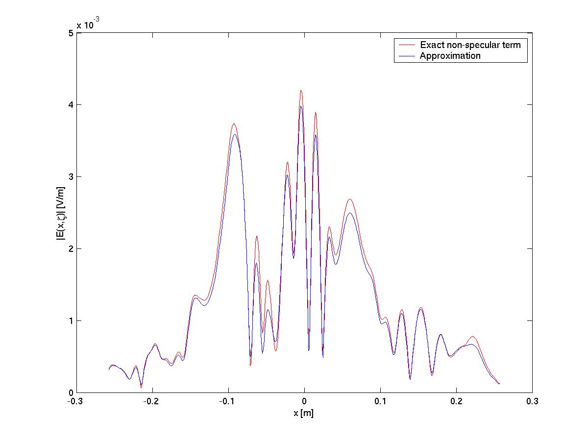
Figure 1: Comparison of exact numerical solution and approximation for scattered field on rough profile $z=\zeta$ with varying impedance $Z=Z_{0}+Z_{r}$ for TE polarisation.

3.2 Plane boundary with varying impedance

We now consider the special case of a planar surface $\zeta(x)\equiv 0$ with variable impedance, using the operator expansion above. We should mention here the elegant method of [1] and that of [2] which also considers ensemble averages and could alternatively be employed. To simplify notation we will denote the operators in this case by ${{\mathcal{A}}}_{0}$ and ${{\mathcal{A}}}_{1}$ so that equation (2) becomes

$$E_{inc}({\bf r})=({{\mathcal{A}}}_{0}+{{{\mathcal{A}}}_{1}})E({\bf r}),$$ (11)

where ${\bf r}$ lies on the surface, ${{\mathcal{A}}}_{0}$ and ${{{\mathcal{A}}}_{1}}$ are now given by

$${{\mathcal{A}}}_{0}(~{}\cdot~{})={1\over 2}(~{}\cdot~{})-\int_{z=0}\left[{\partial G({\bf r},{\bf r}^{\prime})\over\partial z}+{ik_{0}G({\bf r},{\bf r}^{\prime})\over Z_{0}}\right](~{}\cdot~{})dS^{\prime}\rm$$ (12)

and

$${{{\mathcal{A}}}_{1}}(~{}\cdot~{})={ik_{0}\over Z_{0}}\int_{z=0}{Z_{r}(x^{\prime})G({\bf r},{\bf r}^{\prime})\over Z_{0}+Z_{r}(x^{\prime})}(~{}\cdot~{})dS^{\prime}.$$ (13)

Eq. (10) then becomes

$$E({\bf r})\cong{{{\mathcal{A}}}_{0}^{-1}}E_{inc}({\bf r})~{}-~{}{{{\mathcal{A}}}_{0}^{-1}}\left[{{{\mathcal{A}}}_{1}}{{{\mathcal{A}}}_{0}^{-1}}E_{inc}({\bf r})\right].$$ (14)

The solution to (11) represents the total field at $z=0$; from this the field elsewhere can be obtained by writing $E({\bf r})$ as a superposition of plane waves without recourse to the integral (3).

Suppose for the moment that the impedance is constant, $Z=Z_{0}$, so that ${{\mathcal{A}}}_{1}$ vanishes. For an incident plane wave, say $E_{\theta}(x,z)=\exp(ik[\sin\theta x-\cos\theta z])$ at an angle $\theta$ with respect to the normal, the solution is explicitly

$${{{\mathcal{A}}}_{0}^{-1}}E_{\theta}(x,0)~{}=~{}\left[1+R(\alpha)\right]\exp(i\alpha x),$$ (15)

where $\alpha=k\sin\theta$, $\beta=\sqrt{k^{2}-\alpha^{2}}$, and $R$ is the reflection coefficient

$$R(\alpha)={\beta Z_{0}-k_{0}\over\beta Z_{0}+k_{0}}.$$ (16)

Thus ${{\mathcal{A}}}_{0}^{-1}f$ can be found for arbitrary $f(x)$ by expressing $f$ as a superposition of plane waves and applying (15). If impedance variation $Z(x)=Z_{0}+Z_{r}(x)$ is now reintroduced, then (11) has formal solution

$$E({\bf r})=({{\mathcal{A}}}_{0}+{{{\mathcal{A}}}_{1}})^{-1}E_{inc}({\bf r}).$$ (17)

The first term on the right of equation (10) is the known specular reflection from a constant impedance surface at $z=0$; the second models its diffuse modification due to $Z_{r}$, i.e. diffraction effects due to impedance variation.

Specifically, from (15) and (13) we obtain

$${{{\mathcal{A}}}_{1}}({{{\mathcal{A}}}_{0}^{-1}}E_{inc}({\bf r}))={ik_{0}(1+R(\alpha))\over Z_{0}}\int_{z=0}{Z_{r}(x^{\prime})G({\bf r},{\bf r}^{\prime})\over Z_{0}+Z_{r}(x^{\prime})}e^{i\alpha x^{\prime}}dS^{\prime}\rm.$$ (18)

As ${{{\mathcal{A}}}_{0}^{-1}}$ represents reflection by constant impedance, (18) can be thought of as a secondary ‘driving field’ for the diffuse term in (10). This field consists of a set of plane waves determined by the Fourier transform of the integral in (18). An example is shown in Figure 2 comparing this term in (10) with the diffuse part of the exact numerical solution. $Z_{r}$ here has an rms value of around $Z_{0}/4$. (Note that in these simulations the incident field has been tapered to zero at the edges to minimise spurious edge-effects.)

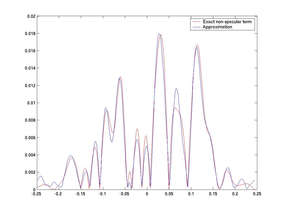
Figure 2: Comparison of exact and approximate solutions for non-specular component of scattered field for a flat surface with varying impedance.

As the solution of ${{{\mathcal{A}}}_{0}^{-1}}$ is known the expression (10) can be evaluated directly, for one or many realisations, and avoids a potentially expensive numerical inversion.

4 Coherent field

In this section we consider statistics of the scattered field (a) when the average is taken over the ensemble of varying impedance functions and the profile is deterministic but arbitrary, and (b) the more general case of a randomly rough surface, taking the average over both impedance and surface profiles.

As the impedance is often known statistically rather than individually, evaluation of the mean field is important. For flat surfaces the mean field with respect to an ensemble of impedance realisations obeys an effective impedance condition, for which an approximation is derived in section (4.1). Thus for an incident plane wave the mean scattered field is specular, but with an ‘effective reflection coefficient’ depending on incident angle. For a given rough surface, the coherent field is no longer specular, and its description is therefore more complex.

4.1 Mean field for plane boundary

We first consider the coherent field for a flat varying-impedance surface, §3.2. A low-order approximation for the mean field due to scattering by the randomly varying impedance is easily derived from the expansion (10) in this case. As $Z_{r}(x)$ is statistically stationary, the coherent field is specular and takes the form of a constant effective impedance whose value we seek. Averaging equation (14) gives the mean field at the surface

$$<E({\bf r})>\cong{{{\mathcal{A}}}_{0}^{-1}}E_{inc}({\bf r})-{{{\mathcal{A}}}_{0}^{-1}}<{{{\mathcal{A}}}_{1}}>{{{\mathcal{A}}}_{0}^{-1}}E_{inc}({\bf r})$$ (19)

as the term ${{{\mathcal{A}}}_{0}^{-1}}E_{inc}({\bf r})$ on which ${{\mathcal{A}}}_{1}$ acts is independent of $Z_{r}$. From equation (13), $<{{{\mathcal{A}}}_{1}}>$ is given by

$$<{{{\mathcal{A}}}_{1}}(~{}\cdot~{})>~{}=~{}{ik_{0}\over Z_{0}}\int_{z=0}~{}{\Lambda}~{}G({\bf r},{\bf r}^{\prime})(~{}\cdot~{})dS^{\prime}~{}=~{}{\Lambda}~{}{ik_{0}\over Z_{0}}\int_{z=0}~{}G({\bf r},{\bf r}^{\prime})(~{}\cdot~{})dS^{\prime}$$ (20)

where

$${\Lambda}~{}=~{}\left<\frac{Z_{r}}{Z_{0}+Z_{r}}\right>~{}=~{}1-Z_{0}\left<\frac{1}{Z_{0}+Z_{r}}\right>$$ (21)

Note that this quantity is a one-point average, which does not depend on the impedance autocorrelation $\rho(\xi)=<Z_{r}(x)Z_{r}(x+\xi)>$. This scalar can be found analytically for a wide range of distributions and in any case numerical averaging is straightforward and rapid for arbitrary statistics. For analytical evaluation, $Z_{r}$ is most commonly assumed to obey a modified form of complex Gaussian distribution. If the distribution is exactly Gaussian then the probability integral has a pole at $Z_{r}=-Z_{0}$, but also a well-defined Cauchy principal value, and can be obtained analytically. However, the singularity at $-Z_{0}$ corresponds to vanishing impedance which may be excluded on physical grounds, and the distribution can be replaced by a Gaussian with cut-off.

Alternatively, to fourth order in the ratio $Z_{r}/Z_{0}$, $\Lambda$ can be written

$$\Lambda~{}\cong~{}\left<{Z_{r}/Z_{0}~{}-~{}Z_{r}^{2}/Z_{0}^{2}~{}+~{}Z_{r}^{3}/Z_{0}^{3}~{}-~{}Z_{r}^{4}/Z_{0}^{4}}\right>$$ (22)

giving a simple high-contrast second order approximation:

$${\Lambda}~{}\cong~{}\left<{Z_{r}^{2}\over Z_{0}^{2}}\right>~{}=~{}-\sigma^{2}_{I}$$ (23)

valid for any distribution, or a fourth order approximation for the Gaussian case:

$${\Lambda}~{}\cong~{}-\left<{Z_{r}^{2}\over Z_{0}^{2}}\right>~{}=~{}-\sigma^{2}_{I}+3\sigma^{4}$$ (24)

In any case, when (20) and (21) are substituted back into equation (19) it is easily seen that the mean field is equivalent to a solution of the original problem with a modified or ‘effective’ constant impedance ${Z_{e}}=Z_{0}+{Z_{mod}}$, with ${Z_{mod}}$ given by ${Z_{mod}}=Z_{0}{\Lambda}/(1-{\Lambda})$. This immediately gives an effective reflection coefficient

$${R_{e}}(\alpha)={\beta{Z_{e}}-k_{0}\over\beta{Z_{e}}+k_{0}}$$ (25)

where

$${Z_{e}}~{}=~{}\frac{Z_{0}}{1-{\Lambda}}.$$ (26)

4.2 Mean field for a rough surface

At a point ${\bf r}$ along a given horizontal line above the surface, the field is related to the surface values via the integral (3), which is written

$$E({\bf r})={\mathcal{C}^{\prime}}E$$ (27)

where ${\mathcal{C}^{\prime}}$ is the integral operator in (3) and the prime is simply to distinguish the operator ${\mathcal{C}}$ evaluated away from the surface from its value along the surface as occurring in (2). If ${\mathcal{C}^{\prime}}$ is split as before into its constant and varying impedance parts ${\mathcal{C}^{\prime}}_{0}$ and ${\mathcal{C}^{\prime}}_{1}$, then, using (10), equation (27) can be written as

$$E = {\mathcal{C}^{\prime}}{\mathcal{C}}^{-1}E_{inc}$$ (28)

$$= ({\mathcal{C}^{\prime}}_{0}+{\mathcal{C}^{\prime}}_{1})({\mathcal{C}}_{0}+{\mathcal{C}}_{1})^{-1}E_{inc}$$

$$\cong ({\mathcal{C}^{\prime}}_{0}+{\mathcal{C}^{\prime}}_{1})({\mathcal{C}}_{0}^{-1}-{\mathcal{C}}_{0}^{-1}{\mathcal{C}}_{1}{\mathcal{C}}_{0}^{-1})E_{inc}$$

$$\cong \left[{\mathcal{C}^{\prime}}_{0}{\mathcal{C}}_{0}^{-1}-{\mathcal{C}^{\prime}}_{0}{\mathcal{C}}_{0}^{-1}{\mathcal{C}}_{1}{\mathcal{C}}_{0}^{-1}+{\mathcal{C}^{\prime}}_{1}{\mathcal{C}}_{0}^{-1})\right]E_{inc}$$

where we have neglected a term of higher order in ${\mathcal{C}}_{1}$. We can now take an ensemble average of (28) with respect to impedance variation, to get the mean modification by impedance variation of the scattered fields.

$$<E({\bf r})>~{}\cong~{}\left[{\mathcal{C}^{\prime}}_{0}{\mathcal{C}}_{0}^{-1}~{}+~{}\overline{{\mathcal{C}^{\prime}}_{1}}{\mathcal{C}}_{0}^{-1}~{}-~{}{\mathcal{C}^{\prime}}_{0}{\mathcal{C}}_{0}^{-1}\overline{{\mathcal{C}}_{1}}{\mathcal{C}}_{0}^{-1})\right]E_{inc}$$ (29)

where ${\bf r}$ is in the medium and for compactness $\overline{{\mathcal{C}}_{1}}$ denotes the mean $<{\mathcal{C}}_{1}>$ and thus

$$\overline{{\mathcal{C}}_{1}}(~{}\cdot~{})~{}=~{}{ik_{0}\over Z_{0}}\int_{z=\zeta(x)}{\Lambda}G({\bf r},{\bf r}^{\prime})(~{}\cdot~{})dS^{\prime}~{}=~{}{\Lambda}~{}{{\mathcal{C}}}_{1},$$ (30)

$\overline{{\mathcal{C}^{\prime}}_{1}}$ defined similarly, and ${\Lambda}$ is given by eq. (21).

Expression (29) gives the mean field for an arbitrary irregular surface with randomly varying impedance, but as $\overline{{\mathcal{C}}_{1}}$, $\overline{{\mathcal{C}^{\prime}}_{1}}$ depend on the surface profile $\zeta(x)$, numerical evaluation cannot in general be avoided. In particular this gives rise to a coherent field spectrum with effective coefficients depending on the surface profile. The approximation (29) is equivalent to the solution $E_{e}$, say, for scattering by the surface $\zeta(x)$ but with constant effective impedance ${Z_{e}}$. This is easily seen by formulating this equivalent problem in terms of integral operators where it becomes

$$E_{e}({\bf r})~{}=~{}({\mathcal{C}^{\prime}}_{0}+{\Lambda}{\mathcal{C}^{\prime}})({\mathcal{C}}_{0}+{\Lambda}{{\mathcal{C}}}_{1})^{-1}E_{inc},$$ (31)

and then solving as before and comparing terms with (29). In terms of the effective field evaluated along the surface which we can denote $E_{se}$, (31) becomes

$$E_{e}({\bf r})~{}=~{}({\mathcal{C}^{\prime}}_{0}+{\Lambda}{\mathcal{C}^{\prime}})~{}E_{se}$$ (32)

In other words the effective field $E_{e}$, i.e. average over impedance realisations, is the solution to the boundary problem given by equations (2) and (3) with varying impedance replaced by effective impedance ${Z_{e}}$:

$$E({\bf r})~{}=~{}~{}\int_{z=\zeta(x)}\left[{\partial G({\bf r},{\bf r}^{\prime})\over\partial n}+{ik_{0}G({\bf r},{\bf r}^{\prime})\over{Z_{e}}}\right]E({\bf r}^{\prime})dS^{\prime}\rm.$$ (33)

4.3 TM case

The results above apply to a TE incident field. It is straightforward to derive equivalent results for TM incidence as follows. Integral equations (2) and 3) for $E$ are replaced by the following equations for the field $H$:

$$H_{inc}({\bf r}_{s})~{}=~{}\frac{1}{2}H({\bf r}_{s})~{}-~{}\int_{z=\zeta(x)}\left[{\partial G({\bf r}_{s},{\bf r}^{\prime})\over\partial n}+{ik_{0}G({\bf r}_{s},{\bf r}^{\prime})(Z_{0}+Z_{r}(x^{\prime}))}\right]H({\bf r}^{\prime})dS^{\prime}\rm.$$ (34)

where ${\bf r}_{s}$ is an arbitrary surface point $(x,\zeta(x))$, and ${\bf r}^{\prime}=(x^{\prime},\zeta(x^{\prime}))$. Elsewhere the field can be written as a boundary integral:

$$H({\bf r})~{}=~{}~{}\int_{z=\zeta(x)}\left[{\partial G({\bf r},{\bf r}^{\prime})\over\partial n}+{ik_{0}G({\bf r},{\bf r}^{\prime})(Z_{0}+Z_{r}(x^{\prime}))}\right]H({\bf r}^{\prime})dS^{\prime}\rm.$$ (35)

Following analogous reasoning we obtain

$$H({\bf r})\cong{{{\mathcal{D}}}_{0}^{-1}}H_{inc}({\bf r})~{}-~{}{{{\mathcal{D}}}_{0}^{-1}}\left[{{{\mathcal{D}}}_{1}}{{{\mathcal{D}}}_{0}^{-1}}H_{inc}({\bf r})\right].$$ (36)

where now

$${{\mathcal{D}}}_{0}(~{}\cdot~{})={1\over 2}(~{}\cdot~{})~{}-~{}\int_{z=\zeta(x)}\left[{\partial G({\bf r},{\bf r}^{\prime})\over\partial n}+{ik_{0}Z_{0}G({\bf r},{\bf r}^{\prime})}\right](~{}\cdot~{})dS^{\prime}\rm.$$ (37)

$${{\mathcal{D}}}_{1}(~{}\cdot~{})~{}=~{}~{}-~{}{ik}\int_{z=\zeta(x)}{Z_{r}(x^{\prime})G({\bf r},{\bf r}^{\prime})}(~{}\cdot~{})dS^{\prime}.$$ (38)

It is immediately clear, however, that when taking the mean with respect to impedance variation the term $<{{\mathcal{D}}}_{1}>$ vanishes so that to this order the effective impedance coincides with $Z_{0}$. Thus ${{\mathcal{D}}}_{1}$ has no effect on $<H>$. The effect on the autocorrelation of $H$ and therefore on mean intensity will be non-zero, but this is beyond the scope of the present study.

4.4 Averaging over rough surfaces

Provided the surface profile and impedance are statistically independent, the above results (32) or (33) can be used to examine the double average $\ll E\gg$ with respect to rough surface and impedance variation. This may be done using results existing in various regimes, which we will not reproduce in detail here. To illustrate this, consider an incident plane wave at angle of $\theta$ for small surface height $\sigma^{2}_{S}<1$. Perturbation theory to first order in surface height can be applied along the lines of [15]. This allows the first order (in $\sigma_{S}$) component to be written as $\zeta(x)u(\theta,{Z_{e}})$ where $u(\theta,{Z_{e}})$ is a known function of incident angle and effective impedance.

From this the field everywhere can be expressed in the standard way in terms of the spectral components via the Fourier transform of $\zeta$, with the function $u(\theta,{Z_{e}})$ present as a multiplying factor. Using this we can obtain coherent field and field correlation within the small surface height regime. Similarly, the mean field for low grazing angle incident waves may be obtained by extending results such as [19] although these require further development.

5 Conclusions

Wave scattering by a rough surface with random spatially varying impedance has been considered. We have sought an efficient method for calculating the field while allowing convenient estimation of the effects of impedance variation and its interaction with the surface profile.

The expressions obtained also provide estimates of the mean field with respect to impedance variation. For rough surfaces these are semi-analytical in the sense that numerical evaluation of integrals is needed. (In the case of a flat surface, for which the coherent field is specular, this takes the form of an effective impedance; this is also approximately true for a given irregular surface, but the behaviour is more complicated because of the non-specular nature of the scattered field.)

For simplicity we have restricted attention to 2-dimensional problems, but the extension to full 3-dimensional scattering is straightforward. Similarly, equivalent results for a TM fields are easily obtained, and the acoustic case follows immediately. A further question which is not addressed here is of the coherent field which results from ensemble of randomly rough surfaces with varying impedance. A key difficulty is that typically when this occurs in practice the roughness and impedance are not statistically independent.

5.1 Acknowledgments

MS gratefully acknowledges partial support for this work under US ONR Global NICOP grant N62909-19-1-2128.

References

- [1] D Dragna and P Blanc-Benon. Sound propagation over the ground with a random spatially-varying surface admittance. The Journal of the Acoustical Society of America, 142(4):2058–2072, 2017.
- [2] Vladimir E Ostashev, D Keith Wilson, and Sergey N Vecherin. Effect of randomly varying impedance on the interference of the direct and ground-reflected waves. The Journal of the Acoustical Society of America, 130(4):1844–1850, 2011.
- [3] K Sarabandi and T Chiu. Electromagnetic scattering from slightly rough surfaces with inhomogeneous dielectric profiles. IEEE Transactions on Antennas and Propagation, 45(9):1419–1430, 1997.
- [4] Yannis Hatziioannou. Scattering of an electromagnetic wave by a conducting surface. Journal of Modern Optics, 46(1):35–47, 1999.
- [5] H Giovannini, M Saillard, and A Sentenac. Numerical study of scattering from rough inhomogeneous films. JOSA A, 15(5):1182–1191, 1998.
- [6] Charles-Antoine Guérin and Anne Sentenac. Second-order perturbation theory for scattering from heterogeneous rough surfaces. JOSA A, 21(7):1251–1260, 2004.
- [7] Ricardo A Depine. Backscattering enhancement of light and multiple scattering of surface waves at a randomly varying impedance plane. JOSA A, 9(4):609–618, 1992.
- [8] VL Brudny and RA Depine. Theoretical study of enhanced backscattering from random surfaces. Optik, 87(4):155–158, 1991.
- [9] DG Blumberg, V Freilikher, I Fuks, Yu Kaganovskii, AA Maradudin, and M Rosenbluh. Effects of roughness on the retroreflection from dielectric layers. Waves in random media, 12(3):279–292, 2002.
- [10] Gary S Brown. Special issue on low-grazing-angle backscatter from rough surfaces. IEEE Transactions on Antennas and Propagation, 46(1):1–2, 1998.
- [11] Y Hatziioannou and M Spivack. Electromagnetic scattering by refractive index variations over a rough conducting surface. Journal of Modern Optics, 48(7):1151–1160, 2001.
- [12] Eric S Li and Kamal Sarabandi. Low grazing incidence millimeter-wave scattering models and measurements for various road surfaces. IEEE Transactions on Antennas and Propagation, 47(5):851–861, 1999.
- [13] JA Ogilvy and Institute of Physics (UK). Theory of wave scattering from random rough surfaces. CRC Press, 1991.
- [14] AG Voronovich. Wave scattering from rough surfaces, volume 17. Springer Science & Business Media, 2013.
- [15] John G Watson and Joseph B Keller. Reflection, scattering, and absorption of acoustic waves by rough surfaces. The Journal of the Acoustical Society of America, 74(6):1887–1894, 1983.
- [16] Narinder Singh Basra. Wave Scattering by Rough Surfaces with Varying Impedances. PhD thesis, University of Cambridge, 2003.
- [17] JA DeSanto. Exact boundary integral equations for scattering of scalar waves from infinite rough interfaces. Wave Motion, 47(3):139–145, 2010.
- [18] David A Kapp and Gary S Brown. A new numerical method for rough-surface scattering calculations. IEEE Transactions on Antennas and Propagation, 44(5):711, 1996.
- [19] M Spivack. Moments of wave scattering by a rough surface. The Journal of the Acoustical Society of America, 88(5):2361–2366, 1990.
- [20] M Spivack, A Keen, J Ogilvy, and C Sillence. Validation of left–right method for scattering by a rough surface. Journal of Modern Optics, 48(6):1021–1033, 2001.
- [21] Connor Brennan, Peter Cullen, and Marissa Condon. A novel iterative solution of the three dimensional electric field integral equation. IEEE Transactions on Antennas and Propagation, 52(10):2781–2785, 2004.