Minimizing relative entropy of path measures under marginal constraints

Abstract.

We study generalizations of the Schrödinger problem in statistical mechanics in two directions: when the density is constrained at more than two times, and when the joint law of the initial and final positions for the particles is prescribed. This is done in agreement with the so-called Brödinger problem recently introduced to regularize Brenier’s variational model for incompressible fluids.

We recover generalizations of the standard factorization result for the Radon-Nikodym derivative of the solution $P$ with respect to the reference measure $R$: this density can be written in terms of an additive functional on the set of constrained times.

The specificity of this work is that we place ourselves in the case when $R$ is Markov (or reciprocal), and that we use Markovian methods rather than classical convex analysis arguments. In this setting, it appears that a natural assumption to be made on the reference measure $R$ is of irreducibility type.

1. Introduction

In this paper, we are interested in the structure of the solutions to a class of entropy minimization problems among path measures: i.e. measures on a path space. More specifically, for any path measures $P\ll R$, the relative entropy of $P$ with respect to $R$ is defined by the formula:

$$H(P|R):=E_{P}\left[\log\frac{\operatorname{d\!}P}{\operatorname{d\!}R}\right],$$

(a precise definition is given at Section 4, in particular when $R$ is unbounded) and we minimize $H(\,\begin{picture}(-1.0,1.0)(-1.0,-3.0)\circle*{3.0}\end{picture}\ |R)$ under various marginal constraints, when the reference path measure $R$ is Markov, or sometimes reciprocal. The definition of a reciprocal path measure and its basic properties are recalled at Definition 3.1; in particular, any Markov measure is reciprocal.

Schrödinger problem

The most classical of these problems is unquestionably the Schrödinger problem and dates back to the 30’s with the original articles [24, 25] by Schrödinger himself. This problem can be informally stated in the following way. Take a population of independent particles uniformly distributed in a box at the initial time, and evolving along Brownian paths. Then at any positive time, one still expects the density of particles to be approximately uniform. But suppose that a very rare event occurs, and that one measures at time $t=0$ and $T>0$ a density of particles far from being uniform (in all this text, we will set without loss of generality $T=1$). Conditionally on this rare event, what is the most likely statistical behavior of the particles of the system? The theory of large deviations gives the following answer. If one calls $R$ the law of the Brownian motion starting from the Lebesgue measure, $n$ the number of particles, $Y_{1},\dots,Y_{n}$ the path of each particle and $\mu,\nu$ the observed densities at times $0$ and $1$, then the empirical measure

$$\frac{1}{n}\sum_{i=1}^{n}\delta_{Y_{i}}$$

must be close to the (unique if exists) minimizer $P$ of the entropy $H(\,\begin{picture}(-1.0,1.0)(-1.0,-3.0)\circle*{3.0}\end{picture}\ |R)$ under the constraints that the initial marginal of $P$ is $\mu$, and its final marginal is $\nu$. The Schödinger problem consists in finding $P$ as a function of $\mu$ and $\nu$. For a precise statement of this problem in a more general setting, see (24). We refer to the survey [18] for both a historical presentation and a precise statement of most of the known results about the Schrödinger problem.

There has been renewed interest in this problem since we understood its link with the theory of optimal transport. In fact, the Schrödinger problem can be seen as a regularized version of the classical quadratic optimal transport (see [21, 20, 18]) and it is now used to compute numerically the solutions to transport problems [10, 5] using the Sinkhorn algorithm [26, 27].

One of the main results of this theory, which is crucial in the applications as it allows the use of the Sinkhorn algorithm, is the factorization property of $P$: there exist $f$ and $g$ two measurable functions such that if $(X_{t})_{t\in[0,1]}$ denotes the canonical process on the set of continuous paths,

$$P=f(X_{0})g(X_{1})R.$$ (1)

This property is classically derived by means of various analytic techniques, sometimes coupled with geometric analogies [6, 9, 14, 7, 22, 23, 16], but we prefer to understand it via a different approach: through Markovian considerations, in the spirit of [19]. More precisely, if $R$ is Markov, then $P$ needs to be Markov (see Lemma 4.1), and the density of $P$ with respect to $R$ needs to be a function of $X_{0}$ and $X_{1}$ (see Theorem 4.5). But under additional irreducibility assumptions on $R$ that will be detailed at Section 3, the only way to satisfy these two properties is to be factorized.

Aim of this paper

The goal of this article is to study how far these arguments can go when further constraints are added. The typical kinds of constraints we want to deal with are

1. marginal constraints, prescribing the law of $X_{t}$ under $P$ for all times $t$ in a given set $\mathcal{T}\subset{[0,1]};$

2. endpoint constraints, prescribing the joint law of $(X_{0},X_{1})$ under $P$.

Our main motivation is the understanding of the so-called Brödinger problem, which is a mixture of the Schrödinger problem just described and the Brenier problem for perfect fluids, presented and studied for the first time in [8]. It consists in finding the minimizer $P$ of relative entropy with respect to the reversible Brownian motion (say on the flat torus $\mathbb{T}^{d}$) when the law of $X_{t}$ under $P$ is prescribed to be the Lebesgue measure at all times $t$ (this is incompressibility), and an endpoint constraint is added. The reader can find information on the Brödinger problem in the recent papers [1, 3, 4].

By adding the constraints (i) and (ii), the factorization property (1) translates formally into

$$\frac{\operatorname{d\!}P}{\operatorname{d\!}R}=\exp\Big{(}\eta(X_{0},X_{1})+A([0,1])\Big{)},$$ (2)

where $\eta$ is measurable and comes from the endpoint constraint, and $A$ is what we call an additive functional only charging $\mathcal{T}$ and comes from the density constraints. We will be more specific in Definition 2.6 below, but $A$ is essentially a random finitely additive measure (or content) which only charges $\mathcal{T}$ and such that for all interval $I$, $A(I)$ only depends on the values of the canonical process $X_{t}$ for $t\in I$. An important observation is that in the case of endpoint constraints (leading to $\eta\neq 0$), $P$ is not Markov, even when $R$ is Markov. This leads to additional difficulties. However, it inherits a more general property, namely the reciprocity, which is still tractable in some cases.

We could not reach formula (2) in full generality; see Remark 5.5. However the main results of this paper are two particular cases. In Theorem 4.5, we treat the case when there is no endpoint constraint (and hence $\eta=0$). In Theorem 5.4, we solve the case when there is an endpoint constraint, but $\mathcal{T}$ is finite.

As a consequence, we do not get a fully satisfactory description of the solutions of the Brödinger problem, but rather of a discrete version of it where only finitely many time marginals are prescribed.

Notation

In the whole paper, $\mathcal{X}$ denotes a Polish space, and the path space $\Omega$ is the set of all continuous curves from $[0,1]$ to $\mathcal{X}.$ For all $t\in[0,1]$, $X_{t}$ (called the canonical process at time $t$) is the evaluation map at time $t$, that is for all $\omega\in\Omega$, $X_{t}(\omega)=\omega(t)$. If $\mathcal{Z}$ is a measurable space, $\mathrm{M}(\mathcal{Z})$ and $\mathrm{P}(\mathcal{Z})$ will be the sets of measures and probability measures on $\mathcal{Z}$ respectively. We recall that when endowed with the topology of uniform convergence, $\Omega$ is a Polish space and its Borel $\sigma$-field is the natural $\sigma$-field $\sigma(X_{t};0\leq t\leq 1)$ generated by the canonical process $(X_{t})_{0\leq t\leq 1}$. In that case, $\mathrm{M}(\Omega)$ and $\mathrm{P}(\Omega)$ stand for the set of Borel measures on $\Omega$ (that we call path measures) and the set of Borel probability measures on $\Omega$.

If $\mathcal{T}$ is a subset of $[0,1]$, we denote $X_{\mathcal{T}}:=(X_{t})_{t\in\mathcal{T}}.$ If $R\in\mathrm{M}(\Omega)$ is conditionable in the sense given in Definition 2.1 and $t_{1},\dots,t_{p}\in[0,1]$, $R_{t_{1},\dots,t_{p}}$ stands for the law of $(X_{t_{1}},\dots,X_{t_{p}})$ under $R$ and $R_{\mathcal{T}}$ stands for the law of $X_{\mathcal{T}}$ under $R$.
More generally, if $\mathcal{Z}_{1}$ and $\mathcal{Z}_{2}$ are two measurable spaces, if $\mathbf{r}\in\mathrm{M}(\mathcal{Z}_{1})$ and if $X:\mathcal{Z}_{1}\to\mathcal{Z}_{2}$ is measurable, then the law of $A$ under $\mathbf{r}$ is denoted by $X_{\#}\mathbf{r}$. If $\mathcal{Z}_{1}$ is Polish and $X_{\#}\mathbf{r}$ is $\sigma$-finite, according to the disintegration theorem, then for $X_{\#}\mathbf{r}$-almost all $x$, the conditional probability $\mathbf{r}(\,\begin{picture}(-1.0,1.0)(-1.0,-3.0)\circle*{3.0}\end{picture}\ |X=x)$ exists. It will be called $\mathbf{r}^{x}$, and $\mathbf{r}^{X}:\mathcal{Z}_{1}\to\mathrm{P}(\mathcal{Z}_{1})$ will be the random variable with measure values almost everywhere defined by

$$\mathbf{r}\mbox{-a.e.}\quad X=x\quad\Rightarrow\quad\mathbf{r}^{X}=\mathbf{r}^{x}.$$

Outline of the paper

Let $R\in\mathrm{M}(\Omega)$ be a fixed reference path measure and $P$ be any path probability measure $P\in\mathrm{P}(\Omega)$ dominated by $R$, i.e. $P$ is absolutely continuous with respect to $R$: $P\ll R$.

At Section 2, we derive characterizations in terms of additive functionals of the Radon-Nikodym density $\operatorname{d\!}P/\operatorname{d\!}R$ in the case when both $P$ and $R$ are Markov. This result is stated at Theorem 2.10: $\operatorname{d\!}P/\operatorname{d\!}R=\exp(A([0,1]))$ for some additive functional $A$.

In Section 3, we ask the following question. Let us assume that for some times $0\leq s<u<t\leq 1$ and some measurable functions $a$, $b$ and $c$, we have:

$$f(X_{s},X_{t})=a(X_{[s,u]})+b(X_{[u,t]}),\qquad R\textrm{-a.e.}$$

In which cases is it true that there are two measurable functions $f_{s}$ and $f_{t}$ such that:

$$f(X_{s},X_{t})=f_{s}(X_{s})+f_{t}(X_{t}),\qquad R\textrm{-a.e.}?$$

This is where the irreducibility of $R$ will come into play, as we will prove in Lemma 3.4 that a sufficient condition is to ask $R$ to be reciprocal (see Definition 3.1) and irreducible (see Assumption 3.3). We also provide counterexamples when one of these two conditions fails to be satisfied.

Then, we explore at Section 4 some consequences for multimarginal entropic minimization problems. In the Schrödinger case, when $R$ is Markov, then $P$ is Markov. If in addition, $R$ is irreducible, the result of Section 3 let us build from the additive functional $A$ given by Theorem 2.10 another additive functional that only charges $\mathcal{T}$ and which coincide with $A$ on the full interval $[0,1]$. This is stated at Theorem 4.5.

In Section 5, we apply Theorem 4.5 to get a description of the solution of the Schrödinger problem when there is a finite number of density constraints (Theorem 5.1). We also get (2) in the Brödinger case (i.e. when adding an endpoint constraint), still when there is a finite number of density constraints (Theorem 5.4). In this case, we can even assume that $R$ is only reciprocal. Theorem 5.4 is a consequence of Theorem 5.1 once noticing that any reciprocal process can be transformed into a Markov process by enlarging the space of states and by "folding" the trajectories; see Lemma 5.3. As far as we know, this argument is new.

In Appendix A, we show how a regularity result by Bakry [2] for two indices martingales let us get for free a regularity property for the quantity $A([s,t])$ with respect to $s$ and $t$ where $A$ is the additive functional given by Theorem 2.10. This regularity is very mild (it is nothing but a generalization of the càdlàg property for classical martingales), but it is sufficient to characterize $A$ by its value on a countable amount of intervals. This is often useful to prove that a property which is true $\forall t,\ \mbox{a.e.}$ is also true $\mbox{a.e.},\ \forall t$.

Finally in Appendix B, we state and prove a standard result in measure theory that shows the relationship between disintegration and absolute continuity of measures. These results are used several times along the proofs.

2. Dominated Markov measures

Basic definitions

Let us begin with the symmetric definition of the Markov property. First of all, we need to make precise what a conditionable path measure is.

Definition 2.1 (Conditionable path measure).

The path measure $Q\in\mathrm{M}(\Omega)$ is said to be conditionable if for all $t\in{[0,1]},$ $Q_{t}$ is a $\sigma$-finite measure on $\mathcal{X}$.

It is shown in [17] that for any conditionable path measure $Q\in\mathrm{M}(\Omega),$ the conditional expectation $E_{Q}[\,\begin{picture}(-1.0,1.0)(-1.0,-3.0)\circle*{3.0}\end{picture}\ |X_{\mathcal{T}}]$ is well-defined for any $\mathcal{T}\subset{[0,1]}.$ This is the reason for this definition.

Definition 2.2 (Markov measure).

A path measure $Q$ on $\Omega$ is said to be Markov if it is conditionable and if for any $t\in[0,1]$ and for any events $A\in\sigma(X_{[0,t]}),B\in\sigma(X_{[t,1]})$

$$Q(A\cap B|X_{t})=Q(A|X_{t})Q(B|X_{t}),\quad Q\textrm{-a.e.}$$ (3)

This means that, knowing the present state $X_{t}$, the future and past informations $\sigma(X_{[t,1]})$ and $\sigma(X_{[0,t]})$, are $Q$-independent.

We will represent the Radon-Nikodym derivatives between laws of Markov processes with the help of contents (see [15]). Contents can be understood as "finitely additive measures".

Definition 2.3 (Content).

Denote by $\mathcal{I}$ the subset of $2^{[0,1]}$ composed by every finite unions of intervals of $[0,1]$. The set $\mathcal{I}$ is clearly closed under finite unions and intersections and under complements of individual elements (such a set is sometimes called a field of sets). We say that a function $\mu$ from $\mathcal{I}$ to $[-\infty,+\infty)$ is a content and we write $\mu\in\mathfrak{C}([0,1])$ if:

• $\mu(\emptyset)=0$,

• for all $I_{1},\,I_{2}\in\mathcal{I}$, $\mu(I_{1}\cup I_{2})=\mu(I_{1})+\mu(I_{2})$ whenever $I_{1}\cap I_{2}=\emptyset$.

Remark 2.4.

It is a simple exercise to show that if $\nu$ is a function from the set of all intervals of the form $[s,t]$ with $s\leq t$ in $[0,1]$ such that for all $s\leq u\leq v\leq t$ in $[0,1]$,

$$\mbox{if }\nu([u,v])=-\infty, \mbox{then }\nu([s,v])=\nu([u,t])=\nu([s,t])=-\infty,$$

else, $$\nu([s,t])=\nu([s,v])+\nu([u,t])-\nu([u,v]),$$

then there is a unique content $\mu$ extending $\nu$. For example, for all $s<t$ in $[0,1]$,

$$\mu((s,t))=\nu([s,t])-\nu(\{s\})-\nu(\{t\}).$$

A typical structure of the contents we will get is the following inner or outer regularity property:

Definition 2.5 (Regular content).

We say that a content $\mu\in\mathfrak{C}([0,1])$ is regular and we write $\mu\in\mathfrak{C}_{r}([0,1])$ if one of the two equivalent following properties is satisfied:

• $\left\{\begin{array}[]{ll}\forall\,0\leq s\leq t\leq 1,\,(s,t)\neq(0,1),&\lim_{\begin{subarray}{c}(\sigma,\tau)\to(s,t)\\ \sigma\leq s,\,\tau\geq t\end{subarray}}\mu([\sigma,\tau])=\mu([s,t]),\\ \forall\,0\leq s<t\leq 1,&\lim_{\begin{subarray}{c}(\sigma,\tau)\to(s,t)\\ \sigma>s,\,\tau<t\end{subarray}}\mu([\sigma,\tau])\mbox{ exists},\end{array}\right.$

• $\left\{\begin{array}[]{ll}\forall\,0\leq s<t\leq 1,&\lim_{\begin{subarray}{c}(\sigma,\tau)\to(s,t)\\ \sigma\geq s,\,\tau\leq t\end{subarray}}\mu\big{(}(\sigma,\tau)\big{)}=\mu\big{(}(s,t)\big{)},\\ \forall\,0\leq s\leq t\leq 1,\,(s,t)\neq(0,1),&\lim_{\begin{subarray}{c}(\sigma,\tau)\to(s,t)\\ \sigma<s,\,\tau>t\end{subarray}}\mu\big{(}(\sigma,\tau)\big{)}\mbox{ exists},\end{array}\right.$

Definition 2.6 (Additive functional).

A mapping $A:\Omega\to\mathfrak{C}([0,1])$ is said to be an additive functional if it is measurable in the sense that for every $I\in\mathcal{I}$, the function $A(I)$ is $\sigma(X_{t},\,t\in I)$-measurable.
We say in addition that $A$ is regular if its values are regular.

The proof of Theorem 2.10, the main result of the present section, relies on the following preliminary Lemma 2.9.

A general lemma

Lemma 2.9 gives the structure of the Radon-Nikodym derivative with respect to $\mathbf{r}$ of a measure $\mathbf{p}\ll\mathbf{r}$ sharing some independence properties with $\mathbf{r}$. The context if the following:

Assumptions 2.7 (Framework for Lemma 2.9).

Consider $\mathcal{Z}$, $\mathcal{Z}_{A}$, $\mathcal{Z}_{B}$ and $\mathcal{Z}_{C}$ four measurable spaces and three measurable mappings $A:\mathcal{Z}\to\mathcal{Z}_{A},$ $B:\mathcal{Z}\to\mathcal{Z}_{B}$ and $C:\mathcal{Z}\to\mathcal{Z}_{C}$. We suppose that the $\sigma$-algebra on $\mathcal{Z}$ is generated by $A$, $B$ and $C$. Take $\mathbf{r}\in\mathrm{M}(\mathcal{Z})$ satisfying:

• the push-forward $C_{\#}\mathbf{r}$ is $\sigma$-finite (in particular, $\mathbf{r}$ is $\sigma$-finite),

• under $\mathbf{r}$, the mappings $A$ and $B$ are independent conditionally on $C$, i.e. for all measurable and nonnegative functions $u$ and $v$,

  $$E_{\mathbf{r}}[u(A)v(B)|C]=E_{\mathbf{r}}[u(A)|C]\>E_{\mathbf{r}}[v(B)|C],\quad\mathbf{r}\mbox{-a.e}.$$

Remark 2.8.

In this setting, it can be shown that for all measurable and nonnegative functions $U:\mathcal{Z}_{A}\times\mathcal{Z}_{C}\to\mathbb{R}_{+}$ and $V:\mathcal{Z}_{B}\times\mathcal{Z}_{C}\to\mathbb{R}_{+}$, we have $\mathbf{r}$-almost everywhere

$$E_{\mathbf{r}}[U(A,C)V(B,C)|C]=E_{\mathbf{r}}[U(A,C)|C]\>E_{\mathbf{r}}[V(B,C)|C].$$

The following Lemma 2.9 will be used during the proof of Theorem 2.10. It is a straightforward extension of [19, Thm. 1.5].

Lemma 2.9.

In the framework of Assumption 2.7, consider $\mathbf{p}\in\mathrm{P}(\mathcal{Z})$ such that $\mathbf{p}\ll\mathbf{r}$.

• If under $\mathbf{p}$, the measurable mappings $A:\mathcal{Z}\to\mathcal{Z}_{A}$ and $B:\mathcal{Z}\to\mathcal{Z}_{B}$ are independent conditionally on $C:\mathcal{Z}\to\mathcal{Z}_{C}$, then there are three nonnegative measurable functions $\alpha:\mathcal{Z}_{A}\times\mathcal{Z}_{C}\to\mathbb{R}_{+}$, $\beta:\mathcal{Z}_{B}\times\mathcal{Z}_{C}\to\mathbb{R}_{+}$ and $\gamma:\mathcal{Z}_{C}\to\mathbb{R}_{+}$ such that $\mathbf{r}$-almost everywhere,

  $$\frac{\operatorname{d\!}\mathbf{p}}{\operatorname{d\!}\mathbf{r}}=\alpha(A,C)\beta(B,C)\gamma(C),$$ (4)

  $$\mathbf{r}\textrm{-a.e.},\quad\gamma(C)\neq 0\Rightarrow E_{\mathbf{r}}[\alpha(A,C)|C]=E_{\mathbf{r}}[\beta(B,C)|C]=1.$$ (5)

  In that case,

  $$\left\{\begin{gathered}\gamma=\frac{\operatorname{d\!}C_{\#}\mathbf{p}}{\operatorname{d\!}C_{\#}\mathbf{r}},\\ \alpha\times\gamma=\frac{\mathrm{d}(A,C)_{\#}\mathbf{p}}{\mathrm{d}(A,C)_{\#}\mathbf{r}},\\ \beta\times\gamma=\frac{\mathrm{d}(B,C)_{\#}\mathbf{p}}{\mathrm{d}(B,C)_{\#}\mathbf{r}}.\end{gathered}\right.$$ (6)

• Conversely, if there are two nonnegative function $\alpha$ and $\beta$ such that

  $$\frac{\operatorname{d\!}\mathbf{p}}{\operatorname{d\!}\mathbf{r}}=\alpha(A,C)\beta(B,C),$$ (7)

  then under $\mathbf{p}$, $A$ and $B$ are independent conditionally on $C$.

Proof.

For the first point, let

$$D:=\frac{\operatorname{d\!}\mathbf{p}}{\operatorname{d\!}\mathbf{r}}.$$

Because $C_{\#}\mathbf{r}$ is $\sigma$-finite, so are $(A,C)_{\#}\mathbf{r}$ and $(B,C)_{\#}\mathbf{r}$. As a consequence, the following functions are well defined $\mathbf{r}$-almost everywhere:

$$\gamma(C):=E_{\mathbf{r}}[D|C],$$

$$\alpha(A,C):=\left\{\begin{array}[]{l l}\displaystyle{\frac{E_{\mathbf{r}}[D|A,C]}{\gamma(C)}}&\mbox{if }\gamma(C)\neq 0,\\ 0&\mbox{else},\end{array}\right.$$

$$\beta(B,C):=\left\{\begin{array}[]{l l}\displaystyle{\frac{E_{\mathbf{r}}[D|B,C]}{\gamma(C)}}&\mbox{if }\gamma(C)\neq 0,\\ 0&\mbox{else}.\end{array}\right.$$

On $\{\gamma(C)\neq 0\}$, it is easily shown that $\mathbf{r}$-almost everywhere,

$$E_{\mathbf{r}}[\alpha(A,C)|C]=E_{\mathbf{r}}[\beta(B,C)|C]=1.$$

Moreover $\mathbf{r}$-almost everywhere on $\{\gamma(C)=0\}$, $D=0$, so the identities

$$E_{\mathbf{r}}[D|A,C]=\alpha(A,C)\gamma(C),$$

$$E_{\mathbf{r}}[D|B,C]=\beta(B,C)\gamma(C)$$

hold $\mathbf{r}$-almost everywhere.

It remains to show

$$D=\alpha(A,C)\beta(B,C)\gamma(C).$$ (8)

Let $u$ be a nonnegative measurable function. Let us compute $E_{\mathbf{p}}[u(A)|C]$. For all measurable and nonnegative function $w$, we have on the one hand:

$$E_{\mathbf{p}}[u(A)w(C)] =E_{\mathbf{p}}[E_{\mathbf{p}}[u(A)|C]w(C)]$$

$$=E_{\mathbf{r}}[DE_{\mathbf{p}}[u(A)|C]w(C)]$$

$$=E_{\mathbf{r}}[E_{\mathbf{r}}[D|C]\>E_{\mathbf{p}}[u(A)|C]w(C)]$$

$$=E_{\mathbf{r}}[\gamma(C)E_{\mathbf{p}}[u(A)|C]w(C)],$$

and on the other hand:

$$E_{\mathbf{p}}[u(A)w(C)] =E_{\mathbf{r}}[Du(A)w(C)]$$

$$=E_{\mathbf{r}}[E_{\mathbf{r}}[Du(A)|C]w(C)]$$

$$=E_{\mathbf{r}}[E_{\mathbf{r}}[E_{\mathbf{r}}[D|A,C]u(A)|C]w(C)]$$

$$=E_{\mathbf{r}}[\alpha(A,C)u(A)|C]\gamma(C)w(C)]$$

So we have $\mathbf{r}$-almost everywhere:

$$\gamma(C)E_{\mathbf{p}}[u(A)|C]=\gamma(C)E_{\mathbf{r}}[\alpha(A,C)u(A)|C],$$

and $\mathbf{p}$-almost everywhere:

$$E_{\mathbf{p}}[u(A)|C]=E_{\mathbf{r}}[\alpha(A,C)u(A)|C].$$

In the same way, for all measurable and nonnegative function $v$, $\mathbf{p}$-almost everywhere:

$$E_{\mathbf{p}}[v(B)|C]=E_{\mathbf{r}}[\beta(B,C)v(B)|C].$$

Using the fact that the $\sigma$-algebra on $\mathcal{Z}$ is $\sigma(A,B,C)$, to get (8), it suffices to show that for all $u$, $v$ and $w$ measurable and nonnegative:

$$E_{\mathbf{p}}[u(A)v(B)w(C)]=E_{\mathbf{r}}[\alpha(A,C)\beta(B,C)\gamma(C)u(A)v(B)w(C)].$$

So let us take $u$, $v$ and $w$ such functions. Because of the independence assumption,

$$E_{\mathbf{p}}[u(A)v(B)w(C)] =E_{\mathbf{p}}[E_{\mathbf{p}}[u(A)v(B)|C]w(C)]$$

$$=E_{\mathbf{p}}[E_{\mathbf{p}}[u(A)|C]\>E_{\mathbf{p}}[v(B)|C]w(C)].$$

And using the formulas computed just before,

$$E_{\mathbf{p}}[u(A)v(B)w(C)]=E_{\mathbf{p}}[E_{\mathbf{r}}[\alpha(A,C)u(A)|C]\>E_{\mathbf{r}}[\beta(B,C)v(B)|C]w(C)].$$

Now, because of Remark 2.8,

$$E_{\mathbf{p}}[u(A)v(B)w(C)] =E_{\mathbf{p}}[E_{\mathbf{r}}[\alpha(A,C)u(A)\beta(B,C)v(B)|C]w(C)]$$

$$=E_{\mathbf{r}}[DE_{\mathbf{r}}[\alpha(A,C)u(A)\beta(B,C)v(B)|C]w(C)]$$

$$=E_{\mathbf{r}}[\gamma(C)E_{\mathbf{r}}[\alpha(A,C)u(A)\beta(B,C)v(B)|C]w(C)]$$

$$=E_{\mathbf{r}}[\alpha(A,C)\beta(B,C)\gamma(C)u(A)v(B)w(C)],$$

and the result follows.

The fact that (4) and (5) imply (6) follows from conditioning (4) with respect to $C$, $(A,C)$ and $(B,C)$ respectively, and from using the independence property of $\mathbf{r}$.

For the second point, we suppose that there are $\alpha$ and $\beta$ such that (7) holds, and we want to show that for all $u$ and $v$ measurable and nonnegative, we have

$$E_{\mathbf{p}}[u(A)v(B)|C]=E_{\mathbf{p}}[u(A)|C]\>E_{\mathbf{p}}[v(B)|C],\quad\mathbf{p}\mbox{-a.e}.$$

This follows from the following, obtained using the same kind of computations as before:

$$\mathbf{p}\textrm{-a.e.},\qquad E_{\mathbf{r}}[\alpha(A,C)|C]>0\quad\mbox{and}\quad E_{\mathbf{r}}[\beta(B,C)|C],$$

$$E_{\mathbf{p}}[u(A)v(B)|C]=\frac{E_{\mathbf{r}}[u(A)\alpha(A,C)|C]E_{\mathbf{r}}[v(B)\beta(B,C)|C]}{E_{\mathbf{r}}[\alpha(A,C)|C]E_{\mathbf{r}}[\beta(B,C)|C]}.$$

It remains to apply this formula first for $v=1$, then for $u=1$, and finally for general $u$ and $v$. ∎

Density of a Markov process

We are now ready to give the main result on the form of the Radon-Nikodym derivative between two laws of Markov processes.

Theorem 2.10.

Let $R$ be a reference Markov measure and let $P\ll R$ a probability measure dominated by $R$ with finite entropy. The three following assertions are equivalent.

1. The measure $P$ is Markov;

2. There is an additive functional $A$ such that

   $$\frac{\operatorname{d\!}P}{\operatorname{d\!}R}=\exp\Big{(}A\big{(}[0,1]\big{)}\Big{)};$$

3. There is a regular additive functional $A$ such that

   $$\frac{\operatorname{d\!}P}{\operatorname{d\!}R}=\exp\Big{(}A\big{(}[0,1]\big{)}\Big{)}.$$

Proof.

We show (3) $\Rightarrow$ (2) $\Rightarrow$ (1) $\Rightarrow$ (3).

$\bullet$ The implication (3) $\Rightarrow$ (2) is obvious.

$\bullet$ For (2) $\Rightarrow$ (1), take $t\in[0,1]$. Then

$$\frac{\operatorname{d\!}P}{\operatorname{d\!}R}=\exp\Big{(}A\big{(}[0,t]\big{)}\Big{)}\exp\Big{(}A\big{(}(t,1]\big{)}\Big{)}.$$

Because of the measurability property of an additive functional, $\exp\big{(}A\big{(}[0,t]\big{)}\big{)}$ is a function of $X_{[0,t]}$ and $\exp\big{(}A\big{(}(t,1]\big{)}\big{)}$ is a function of $X_{[t,1]}$. We can use the second point of Lemma 2.9 with $A=X_{[0,t]}$, $B=X_{[t,1]}$ and $C=X_{t}$ to deduce that under $P$, $X_{[0,t]}$ and $X_{[t,1]}$ are independent conditionally on $X_{t}$. Because this is true for every $t$, $P$ is Markov.

$\bullet$ To prove (1) $\Rightarrow$ (3), set for every $s\leq t$ in $[0,1]$

$$D_{s,t}:=E_{R}\bigg{[}\frac{\operatorname{d\!}P}{\operatorname{d\!}R}\bigg{|}X_{[s,t]}\bigg{]},$$

which are obviously $\sigma(X_{[s,t]})$-measurable. In Appendix A, we show how a result from [2] can be used to show that up to a modification,

$$\forall\,0\leq s\leq t\leq 1,\,(s,t)\neq(0,1),\quad\lim_{\begin{subarray}{c}(\sigma,\tau)\to(s,t)\\ \sigma\leq s,\,\tau\geq t\end{subarray}}D_{\sigma,\tau}=D_{s,t},$$

$$\forall\,0\leq s<t\leq 1,\quad\lim_{\begin{subarray}{c}(\sigma,\tau)\to(s,t)\\ \sigma>s,\,\tau<t\end{subarray}}D_{\sigma,\tau}\mbox{ exists},$$

see Figure 4.
We now define for all $0\leq s\leq t\leq 1$

$$A([s,t]):=\log D_{s,t}\in[-\infty,+\infty).$$

It is well defined for all $\omega$ and all $0\leq s\leq t\leq 1$, and it has the two regularity properties

$$\forall\,0\leq s\leq t\leq 1,\,(s,t)\neq(0,1),\quad\lim_{\begin{subarray}{c}(\sigma,\tau)\to(s,t)\\ \sigma\leq s,\,\tau\geq t\end{subarray}}A([\sigma,\tau])=A([s,t]),$$

$$\forall\,0\leq s<t\leq 1,\quad\lim_{\begin{subarray}{c}(\sigma,\tau)\to(s,t)\\ \sigma>s,\,\tau<t\end{subarray}}A([\sigma,\tau])\mbox{ exists}.$$

Let us follow Remark 2.4. Let $s\leq u\leq v\leq t$ in $[0,1]$ and apply the first point of Lemma 2.9 with $\mathbf{r}=R_{[s,t]}$, $\mathbf{p}=P_{[s,t]}$ (these measures are still Markov), $A=X_{[s,v]}$, $B=X_{[u,t]}$ and $C=X_{[u,v]}$. We end up with three nonnegative measurable functions $\alpha$, $\beta$ and $\gamma$ such that $R$-almost everywhere,

$$\exp\Big{(}A\big{(}[s,t]\big{)}\Big{)}=\frac{\operatorname{d\!}P_{[s,t]}}{\operatorname{d\!}R_{[s,t]}}=\alpha(X_{[s,v]})\times\beta(X_{[u,t]})\times\gamma(X_{[u,v]}),$$

$$\exp\Big{(}A\big{(}[s,v]\big{)}\Big{)}=\frac{\operatorname{d\!}P_{[s,v]}}{\operatorname{d\!}R_{[s,v]}}=\alpha(X_{[s,v]})\times\gamma(X_{[u,v]}),$$

$$\exp\Big{(}A\big{(}[u,t]\big{)}\Big{)}=\frac{\operatorname{d\!}P_{[u,t]}}{\operatorname{d\!}R_{[u,t]}}=\beta(X_{[u,t]})\times\gamma(X_{[u,v]}),$$

$$\exp\Big{(}A\big{(}[u,v]\big{)}\Big{)}=\frac{\operatorname{d\!}P_{[u,v]}}{\operatorname{d\!}R_{[u,v]}}=\gamma(X_{[u,v]}).$$

We easily conclude that $R$-almost everywhere:

$$A\big{(}[u,v]\big{)}=-\infty\quad\Rightarrow\quad A\big{(}[s,t]\big{)}=A\big{(}[s,v]\big{)}=A\big{(}[u,t]\big{)}=-\infty,$$

and that if it is not the case:

$$A\big{(}[s,t]\big{)}=A\big{(}[s,v]\big{)}+A\big{(}[u,t]\big{)}-A\big{(}[u,v]\big{)}.$$

The measurability property for the intervals that are not of the form $[s,t]$ comes from the fact that $\sigma(X_{[s,t]})=\sigma(X_{(s,t)})$, so that for example, $A\big{(}(s,t)\big{)}=A([s,t])-A(\{s\})-A(\{t\})$ is $\sigma(X_{[s,t]})$-measurable and so $\sigma(X_{(s,t)})$-measurable. Finally, the measurability property for all sets of $\mathcal{I}$ is obtained by the additivity property of $A$.
The only remaining thing to show is that this additivity property is valid $R$-almost everywhere for all $0\leq s\leq u\leq v\leq t\leq 1$, and not only for all $0\leq s\leq u\leq v\leq t\leq 1$, $R$-almost everywhere. But it is true $R$-almost everywhere for all $s\leq u\leq v\leq t$ in a countable dense subset of $[0,1]$ and it is easy to pass to the limit thanks to the regularity property of $A$. We set $A\equiv 0$ on the $\omega$’s for which the additivity does not hold for all $0\leq s\leq u\leq v\leq t\leq 1$, so that the property is satisfied for all $\omega$. ∎

Remark 2.11.

This decomposition is far from being unique. To illustrate this, take $(\varphi_{t})_{t\in[0,1]}$ and $(\psi_{t})_{t\in[0,1]}$ two families of measurable functions, such that $\varphi_{1}=\psi_{0}=0$ and such that $R$-almost everywhere, $t\mapsto\varphi_{t}(X_{t})$ is right continuous, left limited and $s\mapsto\psi_{s}(X_{s})$ is left continuous, right limited. Then, if $A$ is an additive functional one can define $B$ on the closed intervals of $[0,1]$ by:

$$B([s,t])=A([s,t])+\varphi_{t}(X_{t})+\psi_{s}(X_{s}).$$

It is easy to check with the help of Remark 2.4 that $B$ can be extended in a regular additive functional, with:

$$A([0,1])=B([0,1]).$$

3. Writing a function as a sum

In this section, we give a framework in which a function of two variables $f=f(x,y)$ can be decomposed as a sum $f(x,y)=\alpha(x)+\beta(y)$. We also provide counter-examples when only a part of the assumptions is satisfied.

The general framework is the following. Suppose that for a path measure $R\in\mathrm{M}(\Omega)$, the following holds:

$$f(X_{s},X_{t})=a(X_{[s,u]})+b(X_{[u,t]}),\quad R\textrm{-a.e.}$$ (9)

where $0\leq s<u<t\leq 1$ and $f$, $a$ and $b$ are $[-\infty,\infty)$-valued measurable functions. This means that a function only depending on the position of the canonical process at times $s$ and $t$ can be decomposed as a sum of a function only depending on the beginning of the trajectory and a function only depending on the end of the trajectory. The question is to know if it is possible to find two measurable functions $f_{s}$ and $f_{t}$ such that:

$$f(X_{s},X_{t})=f_{s}(X_{s})+f_{t}(X_{t}),\quad R\textrm{-a.e.}$$ (10)

We will provide counter-examples to show that it is not always the case: it is necessary to make some assumptions on $R$ to be able to conclude. As it will be revealed by the counter-examples, two types of assumptions are needed.

1. The first assumption is of irreducibility type: there is a non-negligible set of positions $y\in\mathcal{X}$ such that:

   $$R((X_{s},X_{t})\in\,\begin{picture}(-1.0,1.0)(-1.0,-3.0)\circle*{3.0}\end{picture}\ )\ll R((X_{s},X_{t})\in\,\begin{picture}(-1.0,1.0)(-1.0,-3.0)\circle*{3.0}\end{picture}\ |X_{u}=y),$$ (11)

   where $0\leq s\leq u\leq t\leq 1.$ Roughly speaking, for such $y$, if some trajectories of the process go from $X_{s}=x$ to $X_{t}=z$, then there are also trajectories such that $X_{s}=x$ and $X_{t}=z$ with the additional property that $X_{u}=y$.

2. The second assumption concerns the independence properties of $R$ at time $u$: for the positions $y$ satisfying the first assumption it is possible to find for each $x\in\mathcal{X}$ a trajectory $\alpha^{x}$ on the set of times $[s,u]$ joining $x$ to $y$, and for each $z\in\mathcal{X}$ a trajectory $\beta^{z}$ on the set of times $[u,t]$ joining $y$ to $z$, such that:

   $$R(X_{[s,u]}\in\,\begin{picture}(-1.0,1.0)(-1.0,-3.0)\circle*{3.0}\end{picture}\ |X_{u}=y) \ll R(X_{[s,u]}\in\,\begin{picture}(-1.0,1.0)(-1.0,-3.0)\circle*{3.0}\end{picture}\ |X_{[u,t]}=\beta^{X_{t}})\quad R\textrm{-a.e.}$$

   $$R(X_{[u,t]}\in\,\begin{picture}(-1.0,1.0)(-1.0,-3.0)\circle*{3.0}\end{picture}\ |X_{u}=y) \ll R(X_{[u,t]}\in\,\begin{picture}(-1.0,1.0)(-1.0,-3.0)\circle*{3.0}\end{picture}\ |X_{[s,u]}=\alpha^{X_{s}})\quad R\textrm{-a.e.}$$

   In other terms, any beginning of trajectory followed by the process can be extended by the ends of trajectory $\beta$, and any end of trajectories followed by the process can be extended by the beginnings of trajectories $\alpha$

Under these two assumptions, it suffices to choose:

$$f_{s}(X_{s}):=a(\alpha^{X_{s}})\qquad\mbox{and}\qquad f_{t}(X_{t}):=b(\beta^{X_{t}}),$$

in (10). However, the difficulty is in general to find situations where the trajectories $\alpha^{x}$ and $\beta^{z}$ can be built as measurable functions of $x$ and $z$ respectively, and to deal with the negligible sets. It is possible to state very general assumptions under which a measurable selection theorem [28] allows us to achieve these goals (this implies using the axiom of choice). We shall rather follow another path by assuming that $R$ is reciprocal (instead of item 2.), and that it satisfies an additional irreducibility property (see Assumption 3.3 below, instead of item 1.) Under these requirements, assumptions 1. and 2.  hold for any $0\leq s<u<t\leq 1$ and for any $y\in\mathcal{X}$, and the axiom of choice is not necessary.

Counterexamples

Let us provide two counter-examples when assumptions 1. and 2. above are not fulfilled.

1. A path measure $R$ not satisfying the assumption 2.

   

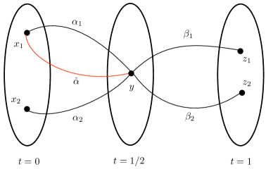
   Figure 1. A counter-example when assumption 2. is dropped

   We consider the simple setting depicted at Figure 1, where only four paths are allowed: the path measure $R$ is uniform on $\left\{\alpha_{1}\beta_{2},\hat{\alpha}\beta_{1},\alpha_{2}\beta_{1},\alpha_{2}\beta_{2}\right\}$ with obvious notation, and it is assumed that $x_{1}\not=x_{2}$, $z_{1}\not=z_{2}$ and $\hat{\alpha}\not=\alpha_{1}$. Clearly the assumption 2 is not satisfied. In particular $R$ fails to be Markov or reciprocal. We exhibit a function $f$ satisfying (9) but not (10).
   The function $f(X_{0},X_{1})$ is specified by:

   $$f(x_{1},z_{1})=1\quad\textrm{and}\quad f(x_{1},z_{2})=f(x_{2},z_{1})=f(x_{2},z_{2})=0,$$

   while the functions $a$ and $b$ are given by:

   $$a(\hat{\alpha})=1,\quad a(\alpha_{1})=a(\alpha_{2})=0,\quad\textrm{and}\quad b(\beta_{1})=b(\beta_{2})=0.$$

   Obviously, we have: $f(X_{0},X_{1})=a(X_{[0,1/2]})+b(X_{[1/2,1]}),\ R\textrm{-a.e.}$, but $f$ fails to satisfy

   $$f(X_{0},X_{1})=f_{0}(X_{0})+f_{1}(X_{1}),\quad R\textrm{-a.e.}$$

   for some functions $f_{0},f_{1}$ since this would imply that

   $$f(x_{1},z_{1}) =f_{0}(x_{1})+f_{1}(z_{1})=f(x_{1},z_{2})-f_{1}(z_{2})+f(x_{2},z_{1})-f_{0}(x_{2})$$

   $$=f(x_{1},z_{2})+f(x_{2},z_{1})-f(x_{2},z_{2})=0,$$

   a contradiction.

2. A Markov measure $R$ not satisfying the assumption 1. We consider the simple setting depicted at Figure 2 where all the drawn paths from left to right are allowed. Note that $R$ can be chosen as a Markov measure. For instance with $R(\alpha_{i}\beta_{j})=p_{i}q_{j}$ where $p_{1}=p_{2}=p_{3}=p_{4}=1/4,$ $q_{1}=1$ and $q_{2}=q_{3}=1/2.$ It is assumed that all the states $x_{1},\dots,z_{3}$ are distinct. Clearly the assumption 1 is not satisfied. Again, we exhibit a function $f$ satisfying (9) but not (10).
   The function $f(X_{0},X_{1})$ is specified by $f(x_{i},z_{j})=f_{ij}$ with

   $$f_{11}=2,f_{12}=2,f_{13}=3,f_{21}=2,f_{22}=3,f_{23}=4.$$

   We see that $f(\alpha_{i}\beta_{j})=a(\alpha_{i})+b(\beta_{j})$ where the functions $a$ and $b$ are given by:

   $$a(\alpha_{1})=1,a(\alpha_{2})=0,a(\alpha_{3})=1,a(\alpha_{4})=1,\quad\textrm{and}\quad b(\beta_{1})=1,b(\beta_{2})=2,b(\beta_{3})=3.$$

   Denote $f_{0}(x_{1})=p,f_{0}(x_{2})=q,f_{1}(z_{1})=r,f_{1}(z_{2})=s,f_{1}(z_{3})=t$ and suppose that (10) holds, that is

   $$p+r=2,\quad q+r=2,\quad p+s=2,\quad q+s=3,\quad p+t=3,\quad q+t=4.$$

   The first two equations imply $p=q$. Plugging this into the third and fourth ones, leads to $2=3.$

   

   Figure 2. Another counter-example when assumption 1. is dropped

The Assumptions 3.3 below are sufficient to prove that (9) implies (10). They require the notion of reciprocal measure.

Reciprocal path measures

Because of the nature of the minimization problems we study, some of the processes are not Markov in general. Still, they satisfy some weaker independence properties, as they are reciprocal in the sense of the following definition:

Definition 3.1 (Reciprocal measure).

A path measure $Q$ on $\Omega$ is called reciprocal if it is conditionable and if it satisfies one of the two following equivalent assertions:

• For any times $0<s<u<1$ and any events $A\in\sigma(X_{[0,s]},X_{[u,1]})$ and $B\in\sigma(X_{[s,u]})$:

  $$Q(A\cap B\mid X_{s},X_{u})=Q(A\mid X_{s},X_{u})Q(B\mid X_{s},X_{u})\quad Q\textrm{-a.e.}.$$ (12)

• For any times $0<s<u<1$ and any events $A\in\sigma(X_{[0,s]}),B\in\sigma(X_{[s,u]}),C\in\sigma(X_{[u,1]})$:

  $$Q(A\cap B\cap C\mid X_{s},X_{u})=Q(A\cap C\mid X_{s},X_{u})Q(B\mid X_{s},X_{u})\quad Q\textrm{-a.e.}.$$ (13)

These properties state that under $Q$, given the knowledge of the canonical process at both times $s$ and $u$, the events inside $[s,u]$ and those outside $(s,u)$ are conditionally independent. It is clearly time-symmetric.

Remarks 3.2.

We recall basic relations between the Markov and reciprocal properties.

1. Any Markov measure is reciprocal. Indeed, let $Q$ be a Markov measure. Then, for any $s,u,A,B$ and $C$ as in the second point of Definition 3.1,

   $$Q(A\cap B\cap C\mid X_{s},X_{u})=Q^{X_{u}}(A\cap B\cap C\mid X_{s})=Q^{X_{u}}(A\mid X_{s})Q^{X_{u}}(B\cap C\mid X_{s})$$

   $$\ =Q^{X_{u}}(A\mid X_{s})Q^{X_{s}}(B\cap C\mid X_{u})=Q^{X_{u}}(A\mid X_{s})Q^{X_{s}}(B\mid X_{u})Q^{X_{s}}(C\mid X_{u})$$

   $$\quad=Q^{X_{u}}(A\mid X_{s})Q^{X_{u}}(C\mid X_{s})Q^{X_{s}}(B\mid X_{u})=Q(A\cap C\mid X_{s},X_{u})Q(B\mid X_{s},X_{u}).$$

2. Conditionally to the initial value or the final value or both of them, a reciprocal measure is Markov. Considering $s=0$ and $A=\Omega$ in the definition of the reciprocal property (13), we see that for all $0\leq u\leq 1,$ $B\in\sigma(X_{[0,u]})$ and $C\in\sigma(X_{[u,1]}),$

   $$Q(B\cap C\mid X_{0},X_{u})=Q(B\mid X_{0},X_{u})Q(C\mid X_{0},X_{u})\quad Q\textrm{-a.e.}$$

   This means that for any reciprocal measure $Q,$ the conditional path measure $Q^{X_{0}}:=Q(\,\begin{picture}(-1.0,1.0)(-1.0,-3.0)\circle*{3.0}\end{picture}\ \mid X_{0})$ is Markov, $Q\textrm{-a.e.}$ Similarly, with $u=1$ and $C=\Omega$ in (13), we see that for all $0\leq s\leq 1,$ $A\in\sigma(X_{[0,s]})$ and $B\in\sigma(X_{[s,1]}),$

   $$Q(A\cap B\mid X_{s},X_{1})=Q(A\mid X_{s},X_{1})Q(B\mid X_{s},X_{1})\quad Q\textrm{-a.e.}$$

   meaning that the conditional path measure $Q^{X_{1}}:=Q(\,\begin{picture}(-1.0,1.0)(-1.0,-3.0)\circle*{3.0}\end{picture}\ \mid X_{1})$ is Markov, $Q\textrm{-a.e.}$

   Because a Markov measure conditioned to its final (or initial) position is still Markov, one gets that if $Q$ is reciprocal, $Q^{X_{0},X_{1}}$ is Markov $Q\textrm{-a.e.}$

Irreducible reciprocal measure

We are ready to state our main assumption.

Assumption 3.3.

Let $R\in\mathrm{M}(\Omega)$ be reciprocal. We say it is irreducible if for all $0\leq s<u<t\leq 1$, we have:

$$R_{s}\otimes R_{u}\otimes R_{t}\ll R_{s,u,t}\ll R_{s}\otimes R_{u}\otimes R_{t}.$$ (14)

(Recall that $R_{t_{1},\dots,t_{k}}$ stands for the law of $(X_{t_{1}},\dots,X_{t_{k}})$ under $R$.) In other terms, the laws $R_{s,u,t}$ and $R_{s}\otimes R_{u}\otimes R_{t}$ are equivalent in the sense of measure theory.

Let us prove that Assumption 3.3 is sufficient to pass from (9) to (10). We will then discuss a little bit further Assumption 3.3: we will see how it can be stated when $R$ is Markov, and how (14) tensorizes.

Lemma 3.4.

Let $R\in\mathrm{M}(\Omega)$ be reciprocal and satisfy Assumption 3.3. Suppose (9) holds for some $0\leq s<u<t\leq 1$, and measurable $f$, $a$ and $b$. Then there exist measurable maps $f_{s}$ and $f_{t}$ such that (10) holds.

Proof.

Taking the conditional expectation in (9) with respect to $(X_{s},X_{u},X_{t})$ leads to:

$$f(X_{s},X_{t}) =E_{R}[f(X_{s},X_{t})|X_{s},X_{u},X_{t}]$$

$$=E_{R}[a(X_{[s,u]})|X_{s},X_{u},X_{t}]+E_{R}[b(X_{[u,t]})|X_{s},X_{u},X_{t}]$$

$$=E_{R}[a(X_{[s,u]})|X_{s},X_{u}]+E_{R}[b(X_{[u,t]})|X_{u},X_{t}],\qquad\qquad R\textrm{-a.e.}$$ (15)

where we used the fact that $R$ is reciprocal to deduce the last line.
Then, let us show that because of Assumption 3.3, formula (11) holds. For this, we use classical results in measure theory stating the behaviour of absolute continuity of measures with respect to conditioning. For the sake of completeness, these results are stated at Proposition B.1 and Lemma B.2. Since $R_{s,u,t}\ll R_{s}\otimes R_{u}\otimes R_{t}$, by Proposition B.1, we have:

$$R_{s,t}\ll R_{s}\otimes R_{t}.$$

In addition, by Lemma B.2, conditioning (14) on $X_{u}$ leads to

$$\phantom{\qquad R\textrm{-a.e.}}R_{s}\otimes R_{t}\ll R((X_{s},X_{t})\in\,\begin{picture}(-1.0,1.0)(-1.0,-3.0)\circle*{3.0}\end{picture}\ |X_{u}),\qquad R\textrm{-a.e.}$$

Bringing together the two last formulas, we get:

$$\phantom{\qquad R\textrm{-a.e.}}R_{s,t}\ll R((X_{s},X_{t})\in\,\begin{picture}(-1.0,1.0)(-1.0,-3.0)\circle*{3.0}\end{picture}\ |X_{u}),\qquad R\textrm{-a.e.},$$

which is (11). Hence, let us pick some $y\in\mathcal{X}$ such that:

$$R_{s,t}\ll R((X_{s},X_{t})\in\,\begin{picture}(-1.0,1.0)(-1.0,-3.0)\circle*{3.0}\end{picture}\ |X_{u}=y),$$ (16)

such that $x\mapsto E[a(X_{[s,u]})|X_{s}=x,X_{u}=y]$ and $z\mapsto E[b(X_{[u,t]})|X_{u}=y,X_{t}=z]$ are well defined $R_{s}\textrm{-a.e.}$ and $R_{t}\textrm{-a.e.}$ respectively, and such that (15) holds $R(\,\begin{picture}(-1.0,1.0)(-1.0,-3.0)\circle*{3.0}\end{picture}\ |X_{u}=y)\textrm{-a.e.}$ (The set of such $y$’s has a full mass with respect to $R_{u}$.) We call:

$$f_{s}(x):=E[a(X_{[s,u]})|X_{s}=x,X_{u}=y]\qquad\mbox{and}\qquad f_{t}(z):=E[b(X_{[u,t]})|X_{u}=y,X_{t}=z].$$

With this choice, by (15):

$$f(x,z)=f_{s}(x)+f_{t}(z),\quad R((X_{s},X_{t})\in\,\begin{picture}(-1.0,1.0)(-1.0,-3.0)\circle*{3.0}\end{picture}\ |X_{u}=y)\textrm{-a.e.}$$

Because of (16), it also holds $R_{s,t}\textrm{-a.e.}$ and the result follows. ∎

The Markov case

In the case when $R$ is Markov, we can restrict ourselves to take a weaker assumption:

Assumption 3.5.

Let $R\in\mathrm{M}(\Omega)$ be Markov. We say it is irreducible if for all $0\leq s<t\leq 1$, we have:

$$R_{s}\otimes R_{t}\ll R_{s,t}\ll R_{s}\otimes R_{t}.$$ (17)

Indeed, we have:

Lemma 3.6.

Let $R\in\mathrm{M}(\Omega)$ be Markov and satisfy Assumption 3.5. Then it satisfies also Assumption 3.3.

In particular, Lemma 3.4 holds for Markov processes satisfying only Assumption 5.3.

Proof.

Let us take $0\leq s<u<t\leq 1$. First, conditioning $R_{u}\otimes R_{t}\ll R_{u,t}\ll R_{u}\otimes R_{t}$ with respect to $X_{u}$ with the help of Lemma B.2 leads to:

$$\hskip 56.9055ptR_{t}\ll R(X_{t}\in\,\begin{picture}(-1.0,1.0)(-1.0,-3.0)\circle*{3.0}\end{picture}\ |X_{u})\ll R_{t},\qquad R\textrm{-a.e.}$$ (18)

Then, we use the disintegration theorem to get the decomposition:

$$R_{s,u,t}=R_{s,u}\otimes R(X_{t}\in\,\begin{picture}(-1.0,1.0)(-1.0,-3.0)\circle*{3.0}\end{picture}\ |X_{s},X_{u})=R_{s,u}\otimes R(X_{t}\in\,\begin{picture}(-1.0,1.0)(-1.0,-3.0)\circle*{3.0}\end{picture}\ |X_{u}),$$

where the second equality is obtained thanks to the Markov property of $R$. The result follows from combining (18) and $R_{s}\otimes R_{u}\ll R_{s,u}\ll R_{s}\otimes R_{u}$. ∎

Next result shows that (17) is indeed an irreducibility requirement in the sense of Markov processes theory. Let us split it into:

$$(\textrm{H}_{1}):\qquad R_{st}\ll R_{s}\otimes R_{t},\quad\forall 0\leq s<t\leq 1;$$

$$(\textrm{H}_{2}):\qquad R_{s}\otimes R_{t}\ll R_{st},\quad\forall 0\leq s<t\leq 1.$$

Proposition 3.7.

Let $R\in\mathrm{M}(\Omega)$ be Markov.

1. Under the assumption $(\textrm{H}_{1})$, for all $0\leq s<t\leq 1,$ we have

   $$R(X_{t}\in\bullet\mid X_{s}=x) =r(s,x;t,\bullet)\,R_{t},\quad\forall x\in\mathcal{X},\ R_{s}\textrm{-a.e.}$$ (19)

   $$R(X_{s}\in\bullet\mid X_{t}=y) =r(s,\bullet;t,y)\,R_{s},\quad\forall y\in\mathcal{X},\ R_{t}\textrm{-a.e.},$$

   where the transition density is given by $\displaystyle{r(s,x;t,y):=\frac{\operatorname{d\!}R_{st}}{\operatorname{d\!}R_{s}\otimes R_{t}}(x,y)}.$

2. If in addition $(\textrm{H}_{2})$ holds, i.e. (17) is satisfied, then $r$ is positive in the sense that

   $$r(s,x;t,y)>0,\quad\forall(x,y),R_{s}\otimes R_{t}\textrm{-a.e.},\quad\forall 0\leq s<t\leq 1.$$ (20)

3. The property (17) is equivalent to the existence of a transition density $r$ satisfying (19) and (20).

Proof.

Apply Lemma B.2 to (H₁). We see that $R(X_{s}\in\bullet\mid X_{t}=y)\ll R_{s}$, for $R_{t}$-almost all $y$ and that $R(X_{t}\in\bullet\mid X_{s}=x)\ll R_{t}$, for $R_{s}$-almost all $x$. This implies that for all $0\leq s<t\leq 1,$ there are measurable functions $\overrightarrow{r}$ and $\overleftarrow{r}$ such that

$$R(X_{t}\in\bullet\mid X_{s}=x) =\overrightarrow{r}(s,x;t,\bullet)\,R_{t},\quad\forall x\in\mathcal{X},\ R_{s}\textrm{-a.e.}$$

$$R(X_{s}\in\bullet\mid X_{t}=y) =\overleftarrow{r}(s,\bullet;t,y)\,R_{s},\quad\forall y\in\mathcal{X},\ R_{t}\textrm{-a.e.}$$

It happens that

$$\overrightarrow{r}(s,x;t,y)=\overleftarrow{r}(s,x;t,y)=r(s,x;t,y),\quad\forall(x,y)\in\mathcal{X}^{2},\ R_{s}\otimes R_{t}\textrm{-a.e.}$$

with $\displaystyle{r(s,x;t,y):=\frac{\operatorname{d\!}R_{st}}{\operatorname{d\!}R_{s}\otimes R_{t}}(x,y),}$ (again, we invoke (H₁)). To see this, note that the joint measure $R_{st}$ writes as

$$R_{st} =r(s,\bullet;t,\bullet)R_{s}\otimes R_{t}$$

$$=R_{s}\otimes R(X_{t}\in\bullet\mid X_{s}=x) \ =\ \overrightarrow{r}(s,\bullet;t,\bullet)R_{s}\otimes R_{t}$$

$$=R_{t}\otimes R(X_{s}\in\bullet\mid X_{t}=y) \ =\ \overleftarrow{r}(s,\bullet;t,\bullet)R_{s}\otimes R_{t}.$$

(When there are two $\bullet$, the first one refers to the first variable, and the second one to the second variable.). Finally, under (H₁) the additional hypothesis (H₂) is equivalent to (20) and statements (b) and (c) are obvious. ∎

The functions $\overrightarrow{r}$ and $\overleftarrow{r}$ are the forward and backward transition densities. By the first the statement of the proposition, it is correct to call $r$ the transition density without mentioning any direction of time.

Tensorization of irreducibility

Here we prove:

Lemma 3.8.

Let $R\in\mathrm{M}(\Omega)$ be a reciprocal process satisfying Assumption 3.3. Then for all $0\leq t_{1}<t_{2}<\dots<t_{k}\leq 1$, we have:

$$R_{t_{1}}\otimes\dots\otimes R_{t_{k}}\ll R_{t_{1},\dots,t_{k}}\ll R_{t_{1}}\otimes\dots\otimes R_{t_{k}}.$$ (21)

Proof.

Let us prove this by induction. We suppose that (21) holds for all $0\leq t_{1}<t_{2}<\dots<t_{k}\leq 1$ for all $3\leq k\leq p$. Then, we choose $0\leq t_{1}<t_{2}<\dots<t_{p+1}\leq 1$. We use once again Lemma B.2 to do the conditioning of

$$R_{t_{1}}\otimes R_{t_{p}}\otimes R_{t_{p+1}}\ll R_{t_{1},t_{p},t_{p+1}}\ll R_{t_{1}}\otimes R_{t_{p}}\otimes R_{t_{p+1}}$$

with respect to $(X_{t_{1}},X_{t_{p}})$. We get

$$\hskip 56.9055ptR_{t_{1}}\otimes R_{t_{p+1}}\ll R(X_{t_{p+1}}\in\,\begin{picture}(-1.0,1.0)(-1.0,-3.0)\circle*{3.0}\end{picture}\ |X_{t_{1}},X_{t_{p}})\ll R_{t_{1}}\otimes R_{t_{p+1}},\qquad R\textrm{-a.e.}$$ (22)

Then, we use the disintegration theorem to get the decomposition:

$$R_{t_{1},\dots,t_{p+1}}=R_{t_{1},\dots,t_{p}}\otimes R(X_{t_{p+1}}\in\,\begin{picture}(-1.0,1.0)(-1.0,-3.0)\circle*{3.0}\end{picture}\ |X_{t_{1}},\dots,X_{t_{p}})=R_{t_{1},\dots,t_{p}}\otimes R(X_{t_{p+1}}\in\,\begin{picture}(-1.0,1.0)(-1.0,-3.0)\circle*{3.0}\end{picture}\ |X_{t_{1}},X_{t_{p}}),$$

where the second equality is obtained thanks to the reciprocity of $R$. The result follows from combining (22) and the induction assumption. ∎

4. Minimizing the relative entropy

The purpose of this section is to prove Theorem 4.5 below, where we prove formula (2) for the solutions of the extended Schrödinger problem, that is in the case when there is no endpoint constraint. Before stating and proving Theorem 4.5, let us define precisely the relative entropy in the case when $R$ is unbounded. Then, we will state two basic properties of the relative entropy which will be useful in the proof of the theorem. Finally, we will introduce the extended Schrödinger problem, and give the result.

The relative entropy with respect to the conditionable path measure $R\in\mathrm{M}(\Omega)$ is defined for all $P\in\mathrm{P}(\Omega)$, by

$$H(P|R):=E_{P}\left[\log\frac{\operatorname{d\!}P}{\operatorname{d\!}R}\right]\in(\infty,\infty].$$

In fact, this definition is not completely rigorous when $R$ is unbounded.

Relative entropy with respect to an unbounded measure

If $R$ is unbounded, one must restrict the definition of $H(\,\begin{picture}(-1.0,1.0)(-1.0,-3.0)\circle*{3.0}\end{picture}\ |R)$ to some subset of $\mathrm{P}(\Omega)$ as follows. As $R$ is assumed to be conditionable, it is a fortiori $\sigma$-finite and there exists some measurable function $W:\Omega\to[0,\infty)$ such that

$$z_{W}:=\int_{\Omega}e^{-W}\operatorname{d\!}R<\infty.$$ (23)

Define the probability measure $R_{W}:=z_{W}^{-1}e^{-W}\,R$ so that $\log(\operatorname{d\!}P/\operatorname{d\!}R)=\log(\operatorname{d\!}P/\operatorname{d\!}R_{W})-W-\log z_{W}.$ It follows that for any $P\in\mathrm{P}(\Omega)$ satisfying $\int_{\Omega}W\operatorname{d\!}P<\infty,$ the formula

$$H(P|R):=H(P|R_{W})-\int_{\Omega}W\operatorname{d\!}P -\log z_{W}\in(-\infty,\infty],$$

$$P\in\mathrm{P}_{W}(\Omega):=\left\{P\in\mathrm{P}(\Omega):E_{P}[W]<\infty\right\}$$

is a meaningful definition of the relative entropy which is coherent in the following sense. If $\int_{\Omega}W^{\prime}\,\operatorname{d\!}P<\infty$ for another measurable function $W^{\prime}:\Omega\to[0,\infty)$ such that $z_{W^{\prime}}<\infty,$ then $H(P|R_{W})-\int_{\Omega}W\operatorname{d\!}P-\log z_{W}=H(P|R_{W^{\prime}})-\int_{\Omega}W^{\prime}\operatorname{d\!}P-\log z_{W^{\prime}}\in(-\infty,\infty]$.
Therefore, $H(P|R)$ is well-defined for any $P\in\mathrm{P}(\Omega)$ such that $\int_{\Omega}W\,\operatorname{d\!}P<\infty$ for some measurable nonnegative function $W$ verifying (23).

A basic lemma from statistical physics

We recall one fundamental easy result from statistical physics. Let $(\mathcal{Z}_{1},\mathbf{r}_{1})$ and $(\mathcal{Z}_{2},\mathbf{r}_{2})$ be two measure spaces with $\mathbf{r}_{1}$ and $\mathbf{r}_{2}$ two probability measures on $\mathcal{Z}_{1}$ and $\mathcal{Z}_{2}$ respectively. Let us call $X_{1},X_{2}$ the projections on the first and second variable respectively in the product space $\mathcal{Z}_{1}\times\mathcal{Z}_{2}$. For any probability measure $\pi\in\mathrm{P}(\mathcal{Z}_{1}\times\mathcal{Z}_{2})$ on the product space $\mathcal{Z}_{1}\times\mathcal{Z}_{2},$ we denote $\pi_{1}:=X_{1}{}_{\#}\pi$ and $\pi_{2}:=X_{2}{}_{\#}\pi$ its marginals on $\mathcal{Z}_{1}$ and $\mathcal{Z}_{2}$ respectively.

Lemma 4.1.

For any $\pi\in\mathrm{P}(\mathcal{Z}_{1}\times\mathcal{Z}_{2})$, we have:

$$H(\pi|\mathbf{r}_{1}\otimes\mathbf{r}_{2})\geq H(\pi_{1}|\mathbf{r}_{1})+H(\pi_{2}|\mathbf{r}_{2})=H(\pi_{1}\otimes\pi_{2}|\mathbf{r}_{1}\otimes\mathbf{r}_{2}).$$

The corresponding equality: $H(\pi|\mathbf{r}_{1}\otimes\mathbf{r}_{2})=H(\pi_{1}|\mathbf{r}_{1})+H(\pi_{2}|\mathbf{r}_{2}),$ holds if and only if $\pi$ is a product measure, i.e. $\pi=\pi_{1}\otimes\pi_{2}.$

Proof.

With the disintegration $\pi=\pi_{1}\otimes\pi^{z_{1}}$ and the additive decomposition of the entropy, we see that

$$H(\pi|\mathbf{r}_{1}\otimes\mathbf{r}_{2}) =H(\pi_{1}|\mathbf{r}_{1})+\int_{\mathcal{Z}_{1}}H(\pi^{z_{1}}\,|\,\mathbf{r}_{2})\,\pi_{1}(\operatorname{d\!}z_{1})$$

$$\geq H(\pi_{1}|\mathbf{r}_{1})+H\Big{(}\int_{\mathcal{Z}_{1}}\pi^{z_{1}}\,\pi_{1}(\operatorname{d\!}z_{1})\,\Big{|}\,\mathbf{r}_{2}\Big{)}$$

$$=H(\pi_{1}|\mathbf{r}_{1})+H(\pi_{2}|\mathbf{r}_{2})=H(\pi_{1}\otimes\pi_{2}|\mathbf{r}_{1}\otimes\mathbf{r}_{2}),$$

where the inequality is a consequence of the convexity of the relative entropy and Jensen’s inequality. Tracking the equality in Jensen’s inequality, we see that $\pi$ must satisfy $\pi^{z_{1}}=\pi_{2}$ for $\pi_{1}$-almost all $z_{1}\in\mathcal{Z}_{1},$ i.e. $\pi=\pi_{1}\otimes\pi_{2}.$ ∎

Let us recall the physical interpretation of this result. Consider two noninteracting random particle systems 1 and 2 respectively governed by the measures $\mathbf{r}_{1}$ and $\mathbf{r}_{2}$. Because of the absence of interaction, the whole system 1+2 is governed by the product measure $\mathbf{r}_{1}\otimes\mathbf{r}_{2}$. Suppose that one observes that the average configurations of 1 and 2 are respectively close to $\pi_{1}$ and $\pi_{2}$. Then, the most likely actual state $\pi_{\textsf{1}+\textsf{2}}$ of the whole system 1+2 is the product $\pi_{1}\otimes\pi_{2},$ meaning that no extra correlation should come into the picture. This result is often quoted as the additivity of the entropy of noninteracting systems, since $H(\pi_{\textsf{1}+\textsf{2}}|\mathbf{r}_{\textsf{1}+\textsf{2}})=H(\pi_{1}|\mathbf{r}_{1})+H(\pi_{2}|\mathbf{r}_{2}).$

A basic lemma from theoretical statistics

Next result is well-known in theoretical statistics where it gives rise to the notion of exhaustive statistics of a dominated statistical model, see [11]. Let $\mathcal{Z}$ and $\SS$ be two Polish spaces equipped with their Borel $\sigma$-fields and $S:\mathcal{Z}\to\SS$ a measurable mapping. Consider a positive $\sigma$-finite measure $\mathbf{r}$ and a probability measure $\mathbf{p}$ on $\mathcal{Z}$ such that $\mathbf{p}\ll\mathbf{r}$. We denote $\mathbf{r}_{S}:=S_{\#}\mathbf{r}$ and $\mathbf{p}_{S}:=S_{\#}\mathbf{p}$ and we assume that $\mathbf{r}_{S}$ is also a $\sigma$-finite measure on $\SS$ to be able to consider the conditional measure $\mathbf{r}(\,\begin{picture}(-1.0,1.0)(-1.0,-3.0)\circle*{3.0}\end{picture}\ |S)$. Because of Proposition B.1, we have $\mathbf{p}_{s}\ll\mathbf{r}_{S}$.

Lemma 4.2.

Let $\mathbf{r},\mathbf{p}$ and $S$ as above. The two following assertions are equivalent:

1. the following conditional laws coincide:

   $$\mathbf{p}(\,\begin{picture}(-1.0,1.0)(-1.0,-3.0)\circle*{3.0}\end{picture}\ |S)=\mathbf{r}(\,\begin{picture}(-1.0,1.0)(-1.0,-3.0)\circle*{3.0}\end{picture}\ |S),\quad\mathbf{p}\textrm{-a.e.}$$

2. There is a measurable map $f\SS\to[0,\infty)$ such that:

   $$\frac{\operatorname{d\!}\mathbf{p}}{\operatorname{d\!}\mathbf{r}}=f\circ S,\ \mathbf{r}\textrm{-a.e.}$$

In this case, we have $\displaystyle{f=\frac{\operatorname{d\!}\mathbf{p}_{S}}{\operatorname{d\!}\mathbf{r}_{S}}}$.

Proof.

$\bullet$ Proof of (i)$\Rightarrow$(ii). The statement: "$\mathbf{p}(\,\begin{picture}(-1.0,1.0)(-1.0,-3.0)\circle*{3.0}\end{picture}\ |S)=\mathbf{r}(\,\begin{picture}(-1.0,1.0)(-1.0,-3.0)\circle*{3.0}\end{picture}\ |S),\ \mathbf{p}\textrm{-a.e.}$" is equivalent to $\mathbf{p}=\int_{\SS}\mathbf{r}(\,\begin{picture}(-1.0,1.0)(-1.0,-3.0)\circle*{3.0}\end{picture}\ |S=s)\,\mathbf{p}_{S}(\operatorname{d\!}s)$. Hence, for any bounded measurable function $u:\mathcal{Z}\to\mathbb{R},$

$$E_{\mathbf{p}}[u] =\int_{\SS}E_{\mathbf{r}}[u|S=s]\,\mathbf{p}_{S}(\operatorname{d\!}s)=\int_{\SS}E_{\mathbf{r}}[u|S=s]\frac{\operatorname{d\!}\mathbf{p}_{S}}{\operatorname{d\!}\mathbf{r}_{S}}(s)\,\mathbf{r}_{S}(\operatorname{d\!}s)$$

$$=\int_{\SS}E_{\mathbf{r}}\Big{[}\frac{\operatorname{d\!}\mathbf{p}_{S}}{\operatorname{d\!}\mathbf{r}_{S}}(s)\ u\Big{|}S=s\Big{]}\,\mathbf{r}_{S}(\operatorname{d\!}s)=\int_{\mathcal{Z}}\frac{\operatorname{d\!}\mathbf{p}_{S}}{\operatorname{d\!}\mathbf{r}_{S}}(S)\ u\operatorname{d\!}\mathbf{r}$$

which means $\displaystyle{\frac{\operatorname{d\!}\mathbf{p}}{\operatorname{d\!}\mathbf{r}}}=\frac{\operatorname{d\!}\mathbf{p}_{S}}{\operatorname{d\!}\mathbf{r}_{S}}(S).$

$\bullet$ Proof of (ii)$\Rightarrow$(i). For any bounded measurable function $u:\mathcal{Z}\to\mathbb{R},$

$$E_{\mathbf{p}}[u]=\int_{\mathcal{Z}}f(S)\ u\operatorname{d\!}\mathbf{r}=\int_{\SS}E_{\mathbf{r}}[u|S=s]f(s)\,\mathbf{r}_{S}(\operatorname{d\!}s)=\int_{\SS}E_{\mathbf{r}}[u|S=s]\,(f\mathbf{r}_{S})(\operatorname{d\!}s).$$

Choosing $u=v\circ S$ with $v:\SS\to\mathbb{R}$ bounded and measurable leads to $E_{\mathbf{p}_{S}}(v)=\int_{\SS}v\,\mathrm{d}(f\mathbf{r}_{S})$. This means that $\displaystyle{f=\frac{\operatorname{d\!}\mathbf{p}_{S}}{\operatorname{d\!}\mathbf{r}_{S}}}.$ Finally, identifying $E_{\mathbf{p}}[u\ v(S)]=\int_{\SS}E_{\mathbf{p}}[u|S=s]v(s)\,\mathbf{p}_{S}(\operatorname{d\!}s)$ with $E_{\mathbf{p}}[u\ v(S)]=\int_{\SS}E_{\mathbf{r}}[u|S=s]v(s)\,\mathbf{p}_{S}(\operatorname{d\!}s)$ gives us $\mathbf{p}(\,\begin{picture}(-1.0,1.0)(-1.0,-3.0)\circle*{3.0}\end{picture}\ |S)=\mathbf{r}(\,\begin{picture}(-1.0,1.0)(-1.0,-3.0)\circle*{3.0}\end{picture}\ |S),\ \mathbf{p}\textrm{-a.e.}$ ∎

Statement of the extended Schrödinger problem

We are interested in the marginal constraint $P_{t}=\mu_{t}$ for all $t\in\mathcal{T}\subset[0,1]$, where $\mu_{t}\in\mathrm{P}(\mathcal{X}),\ t\in\mathcal{T}.$ The entropy minimization problem we consider is:

$$H(P|R)\to\textrm{min};\qquad P\in\mathrm{P}(\Omega):P_{t}=\mu_{t},\forall t\in\mathcal{T}.$$ (24)

It is a generalization of the dynamical Schrödinger problem corresponding to $\mathcal{T}=\left\{0,1\right\}$. The properties of the relative entropy lead to the following existence result stating that a unique solution to this problem exists if and only if there is at least one competitor. Results concerning the existence of such competitors can be found for instance in [12, 14], but we do not wish to develop them here.

Proposition 4.3.

Problem (24) admits a solution if and only if there exists some $Q\in\mathrm{P}(\Omega)$ such that $Q_{t}=\mu_{t}$ for all $t\in\mathcal{T}$ and $H(Q|R)<\infty.$ In this case, the solution $P$ is unique.

Sketch of proof. This argument is standard. The conclusion follows from the three following facts:

1. As $\Omega$ is a Polish space, the relative entropy $H(\,\begin{picture}(-1.0,1.0)(-1.0,-3.0)\circle*{3.0}\end{picture}\ |R)$ has compact sublevels on $\mathrm{P}(\Omega)$ with respect to the usual narrow topology $\sigma(\mathrm{P}(\Omega),\mathrm{C}_{b}(\Omega))$.

2. The constraint set $\left\{P\in\mathrm{P}(\Omega);P_{t}=\mu_{t},\ t\in\mathcal{T}\right\}$ is closed.

3. The existence of $Q$ in our assumption implies that the compact set

   $$\left\{P\in\mathrm{P}(\Omega);P_{t}=\mu_{t},\ t\in\mathcal{T}\}\cap\{P\in\mathrm{P}(\Omega);H(P|R)\leq H(Q|R)\right\}$$

   is not empty. Hence, it contains a solution.

4. Uniqueness follows from the strict convexity of the relative entropy, and from the convexity of the constraint set.

Remark 4.4 (The closure of $\mathcal{T}$).

For all $P\in\mathrm{P}(\Omega)$, $t\mapsto P_{t}$ is continuous. For this reason, the extended Schrödinger problem (24) only admits solution if $t\in\mathcal{T}\mapsto\mu_{t}$ can be extended into a continuous map on $[0,1]$. In particular, it must admit limits for $t\in\partial\mathcal{T}$, and if so, for all $t\in\partial\mathcal{T}$, the property:

$$P_{t}=\lim_{\begin{subarray}{c}s\to t\\ s\in\mathcal{T}\end{subarray}}\mu_{s}$$

holds automatically.

Hence, it is clear that we can suppose without loss of generality that $\mathcal{T}$ is closed. This is systematically assumed in the following.

Factorization result for the extended Schrödinger problem

We are now ready to state the central result of this article: a solution to this type of extended Schrödinger problems is Markov, and the additive functional given by Theorem 2.10 cancels outside $\mathcal{T}$. Even if in next Section 5 we only apply this result to the case when $\mathcal{T}$ is finite, we think that this result is interesting in the general case.

Theorem 4.5.

Suppose that $R$ is Markov, and that problem (24) admits a (unique) solution $P$. Then $P$ is Markov. In particular, there exists a regular additive functional $A$ such that:

$$\frac{\operatorname{d\!}P}{\operatorname{d\!}R}=\exp\Big{(}A\big{(}[0,1]\big{)}\Big{)}.$$ (25)

Moreover, $A([0,1])$ is $\sigma(X_{\mathcal{T}})$-measurable, and for any interval $I\subset[0,1]$ with $\inf I=s$ and $\sup I=t$, $A(I)$ is $\sigma(X_{s},X_{t},X_{I\cap\mathcal{T}})$-measurable.

Besides, if $\mathcal{T}$ is closed, and if $R$ satisfies the irreducibility Assumption 3.5, there exists an additive functional $A$ (which is not regular anymore; see Remark 4.6) with the following additional property: for all interval $I\subset[0,1]$:

$$I\cap\mathcal{T}=\emptyset\quad\Rightarrow\quad A(I)=0.$$ (26)

In this case, for all interval $I\subset[0,1]$, $A(I)$ is $X_{I\cap\mathcal{T}}$-measurable.

If the complementary of $\mathcal{T}$ is a finite union of disjoint open intervals, then this additive functional $A$ is regular.

Remark 4.6.

As we saw in the statement of Theorem 4.5, for a general $\mathcal{T}$ we do not know how to access to a regular additive functional satisfying (26). However, the $A$ we are going to build is in some sense "regular up to a closed set of empty interior". More precisely if one writes the complementary of $\mathcal{T}$ as a countable union of disjoint open intervals:

$$\mathcal{T}^{c}=\bigsqcup_{i\in\Lambda}(s_{i},t_{i}),$$

then regularity fails at the accumulation points of the endpoints $\{s_{i},t_{i}\,|\,i\in\Lambda\}$. In particular, if the union is finite, regularity is preserved, as stated in Theorem 4.5.

Proof.

$\bullet$  The solution $P$ is Markov. We denote for any $0<s<1$, $Q^{X_{s}}:=Q(\,\begin{picture}(-1.0,1.0)(-1.0,-3.0)\circle*{3.0}\end{picture}\ |X_{s}),$ $Q^{X_{s}}_{\leftarrow}:=(X_{[0,s]})_{\#}Q^{X_{s}}$ and $Q^{X_{s}}_{\rightarrow}:=(X_{[s,1]})_{\#}Q^{X_{s}}$ for any conditionable $Q\in\mathrm{M}(\Omega).$ Let us also define for any $Q\in\mathrm{P}(\Omega),$

$$\widetilde{Q}^{s}:=\int_{\mathcal{X}}[Q^{X_{s}=x}_{\leftarrow}\otimes Q^{X_{s}=x}_{\rightarrow}]\,Q_{s}(\operatorname{d\!}x)\in\mathrm{P}(\Omega).$$

Referring to (3), we have to prove that for all $0<s<1,$ the solution $P$ satisfies

$$P^{X_{s}}=P^{X_{s}}_{\leftarrow}\otimes P^{X_{s}}_{\rightarrow},\quad P\textrm{-a.e.}$$

or equivalently

$$\widetilde{P}^{s}=P.$$

To this purpose, it is sufficient to show that

1. for any $Q\in\mathrm{P}(\Omega),$ we have

   $$H(\widetilde{Q}^{s}|R)\leq H(Q|R),\quad\forall 0<s<1$$

   with equality if and only if $Q=\widetilde{Q}^{s},$

2. and also that

   $$\widetilde{Q}_{t}^{s}=Q_{t}\in\mathrm{P}(\mathcal{X}),\quad\forall 0\leq t\leq 1,\ 0<s<1.$$

Let us fix $s$ and $Q\in\mathrm{P}(\Omega)$ and start proving (i). By the additive decomposition of the entropy,

$$H(Q|R) =H(Q_{s}|R_{s})+\int_{\mathcal{X}}H(Q^{X_{s}=x}\,|\,R^{X_{s}=x})\,Q_{s}(\operatorname{d\!}x)$$

$$=H(Q_{s}|R_{s})+\int_{\mathcal{X}}H(Q^{X_{s}=x}\,|\,R^{X_{s}=x}_{\leftarrow}\otimes R^{X_{s}=x}_{\rightarrow})\,Q_{s}(\operatorname{d\!}x)$$

$$\geq H(Q_{s}|R_{s})+\int_{\mathcal{X}}H(Q^{X_{s}=x}_{\leftarrow}\otimes Q^{X_{s}=x}_{\rightarrow}\,|\,R^{X_{s}=x}_{\leftarrow}\otimes R^{X_{s}=x}_{\rightarrow})\,Q_{s}(\operatorname{d\!}x),$$

where at the second equality we use the assumed Markov property of $R$ and at the last inequality we apply Lemma 4.1 with $\mathbf{r}_{1}=R^{X_{s}=x}_{\leftarrow}$ and $\mathbf{r}_{2}=R^{X_{s}=x}_{\rightarrow}.$ In addition, Lemma 4.1 tells us that if the identity:

$$Q^{X_{s}}=Q^{X_{s}}_{\leftarrow}\otimes Q^{X_{s}}_{\rightarrow},\quad Q\textrm{-a.e.}$$

fails, then the last inequality is strict. This proves (i).

It remains to prove (ii), i.e.  the operation $Q\leadsto\widetilde{Q}^{s}$ does not alter the marginals. For any bounded measurable function $a:\mathcal{Z}\to\mathbb{R}$ and any $t\in[0,s],$

$$E_{Q}[a(X_{t})]=\int_{\mathcal{X}}E_{Q^{X_{s}=x}_{\leftarrow}}[a(X_{t})]\,Q_{s}(\operatorname{d\!}x)=\int_{\mathcal{X}}E_{Q^{X_{s}=x}_{\leftarrow}\otimes Q^{X_{s}=x}_{\rightarrow}}[a(X_{t})]\,Q_{s}(\operatorname{d\!}x)=E_{\widetilde{Q}^{s}}[a(X_{t})]$$

and for any $t\in[s,1]$ a similar reasoning still works:

$$E_{Q}[a(X_{t})]=\int_{\mathcal{X}}E_{Q^{X_{s}=x}_{\rightarrow}}[a(X_{t})]\,Q_{s}(\operatorname{d\!}x)=\int_{\mathcal{X}}E_{Q^{X_{s}=x}_{\leftarrow}\otimes Q^{X_{s}=x}_{\rightarrow}}[a(X_{t})]\,Q_{s}(\operatorname{d\!}x)=E_{\widetilde{Q}^{s}}[a(X_{t})].$$

This proves (ii).
Therefore, the solution $P$ is Markov and we know with Theorem 2.10 that this is equivalent to:

$$\frac{\operatorname{d\!}P}{\operatorname{d\!}R}=\exp\Big{(}A\big{(}[0,1]\big{)}\Big{)}$$

for some regular additive functional $A$.
$\bullet$  Measurability. To prove that $A\big{(}[0,1]\big{)}$ is $\sigma(X_{\mathcal{T}})$-measurable, it is enough to show that

$$\frac{\operatorname{d\!}P}{\operatorname{d\!}R}\mbox{ is }X_{\mathcal{T}}\mbox{-measurable}.$$ (27)

Using the additive decomposition of the entropy, we see that

$$H(P|R)=H(P_{\mathcal{T}}|R_{\mathcal{T}})+\int_{\mathcal{Z}^{\mathcal{T}}}H(P^{X_{\mathcal{T}}=\zeta}|R^{X_{\mathcal{T}}=\zeta})\,P_{\mathcal{T}}(\operatorname{d\!}\zeta)$$

and it follows that

$$\widehat{P}:=\int_{\mathcal{Z}^{\mathcal{T}}}R^{X_{\mathcal{T}}=\zeta}\,P_{\mathcal{T}}(\operatorname{d\!}\zeta)\in\mathrm{P}(\Omega)$$

satisfies

$$H(\widehat{P}|R)=H(P_{\mathcal{T}}|R_{\mathcal{T}})\leq H(P|R).$$

We also have $\widehat{P}_{\mathcal{T}}=P_{\mathcal{T}}$, implying a fortiori that $\widehat{P}_{t}=P_{t}$ for all $t\in\mathcal{T}.$ As a consequence, the solution $P$ of the Schrödinger problem satisfies $P=\widehat{P}.$ In other words $P^{X_{\mathcal{T}}}=R^{X_{\mathcal{T}}},$ $P\textrm{-a.e.}$ and we know with Lemma 4.2 that this is equivalent to (27).
The proof of the fact that for an interval $I\subset[0,1]$ with $\inf I=s$ and $\sup I=t$, $A(I)$ is $\sigma(X_{s},X_{t},X_{I\cap\mathcal{T}})$-measurable follows the same lines by noticing that the restriction $X_{I}{}_{\#}P$ of $P$ to $I$ is a solution of the extended Schrödinger problem (24) between the times $s$ and $t$:

$$H(Q|X_{\overline{I}}{}_{\#}R)\to\textrm{min};\quad P\in\mathrm{P}\big{(}\Omega_{\overline{I}}):Q_{u}=\mu_{u},\forall u\in I\cap\mathcal{T},\,Q_{s}=P_{s},\,Q_{t}=P_{t},$$

where $\Omega_{I}$ is the set of paths on the time interval $\overline{I}$, with values in $\mathcal{X}$.
$\bullet$  Construction of a version of $A([0,1])$ canceling outside $\mathcal{T}$. Now, in case $R$ satisfies the irreducibility Assumption 3.5, the goal is to build an additive functional $\tilde{A}$ such that $\tilde{A}([0,1])=A([0,1])$ and such that (26) holds for $\tilde{A}$.

First, we can suppose without loss of generality that $0,1\in\mathcal{T}$. Indeed, if it is not the case, by calling $s:=\min\mathcal{T}$ and $t:=\max\mathcal{T}$, it suffices to prove the result for the restriction $P_{[s,t]}$ and $R_{[s,t]}$ and then to extend the obtained additive functional by $0$ on the intervals included outside $[s,t]$.

Here is the procedure to define $\tilde{A}$ from $A$. Let us write the complementary set of $\mathcal{T}$ as a countable union of disjoint open intervals:

$$\mathcal{T}^{c}=\bigsqcup_{i\in\Lambda}(s_{i},t_{i}).$$

For each $i\in\Lambda$, call $u_{i}:=(s_{i}+t_{i})/2$. We have:

$$A((s_{i},t_{i}))=A((s_{i},u_{i}])+A((u_{i},t_{i})).$$

but by the first part of the theorem, $A((s_{i},t_{i}))$ is $\sigma(X_{s_{i}},X_{t_{i}})$-measurable, so that we are in the framework of Lemma 3.4: there exist $\alpha_{i},\beta_{i}$ such that $R\textrm{-a.e.}$,

$$A((s_{i},t_{i}))=\alpha_{i}(X_{s_{i}})+\beta_{i}(X_{t_{i}}).$$

Let us define $\tilde{A}([s,t])$ for $s\leq t\in[0,1]$ in the following way. We call $\varphi(s):=t_{i}$ if $s_{i}\leq s\leq t_{i}$ and $\varphi(s)=s$ otherwise. Correspondingly, we call $\psi(t)=s_{i}$ if $s_{i}\leq t\leq t_{i}$ and $\psi(t)=t$ otherwise. Then, we set:

$$\tilde{A}\big{(}[s,t]\big{)}:=\mathbf{1}_{\{\varphi(s)\leq\psi(t)\}}A\big{(}[\varphi(s),\psi(t)]\big{)}+\sum_{i\in\Lambda}\mathbf{1}_{\{s_{i}<s\leq t_{i}\leq t\}}\beta_{i}(X_{t_{i}})+\sum_{j\in\Lambda}\mathbf{1}_{\{s\leq s_{j}\leq t<t_{j}\}}\alpha_{j}(X_{s_{j}}).$$

(Note that for each sum, at most one term is nonzero so that this formula is well defined.) Clearly $\tilde{A}([0,1])=A([0,1])$, $\tilde{A}([s,t])$ is $X_{[s,t]}$-measurable, and for any interval $I\subset\mathcal{T}^{c}$, this formula leads to $\tilde{A}(I)=0$.

Let us prove that $\tilde{A}$ is an additive functional. Once again, we follow Remark 2.4. Let us take $0\leq s\leq u\leq v\leq t$ and suppose that $\tilde{A}([u,v])=-\infty$. We show that:

$$\tilde{A}([s,v])=\tilde{A}([u,t])=\tilde{A}([s,t])=-\infty.$$ (28)

It means that $\varphi(u)\leq\psi(v)$ and that one of the following holds:

• $A([\varphi(u),\psi(v)])=-\infty$,

• there exists $i\in\Lambda$ such that $s_{i}<u\leq t_{i}\leq v$ and $\beta_{i}(X_{t_{i}})=-\infty$,

• there exists $i\in\Lambda$ such that $u\leq s_{i}\leq v<t_{i}$ and $\alpha_{i}(X_{s_{i}})=-\infty$.

In the first case, as $[\varphi(u),\psi(v)]$ is a subset of $[\varphi(s),\psi(v)]$, $[\varphi(u),\psi(t)]$ and $[\varphi(s),\psi(t)]$, $\tilde{A}=-\infty$ on this three intervals, so that (28) holds.
In the second case, $\beta_{i}(X_{t_{i}})$ also intervenes in the definition of $\tilde{A}([u,t])$, which is hence infinite. Then, either $s_{i}<s$, and so $\beta_{i}(X_{t_{i}})$ also intervenes in the definition of $\tilde{A}([s,v])$, and $\tilde{A}([s,t])$ which let us conclude, or $s\leq s_{i}$ so that $(s_{i},t_{i})$ is a subset of both $[\varphi(s),\psi(v)]$ and $[\varphi(s),\psi(t)]$. In this last case, we conclude by using the fact that thanks to (28), $A((s_{i},t_{i}))=-\infty$.
The third case is treated in the same way.

Now, we suppose that $\tilde{A}([u,v])$ is finite and we want to show:

$$\tilde{A}([s,t])+\tilde{A}([u,v])=\tilde{A}([s,v])+\tilde{A}([u,t]).$$ (29)

There are several cases to deal with, let us treat them one by one.

• If there is some $i\in\Lambda$ such that $[s,t]\subset(s_{i},t_{i})$, then every term in (29) is zero.

• If $s,u$ are in $\mathcal{T}\backslash(\cup_{i}(s_{i},t_{i}])$, and $v,t$ are in $\mathcal{T}\backslash(\cup_{i}[s_{i},t_{i}))$ then (29) is a consequence for the same formula with $A$ instead of $\tilde{A}$.

• If for instance for some $i\in\Lambda$, $s_{i}<s\leq t_{i}\leq v$, then $\beta_{i}(X_{t_{i}})$ appears once on the left-hand side of (29), in the definition of $\tilde{A}([s,t])$, and once on the right-hand side, in the definition of $\tilde{A}([s,v])$. An analogous argument allows us to treat the cases where $u\leq s_{i}\leq t<t_{i}$, $s_{i}<u\leq t_{i}\leq v\leq t$ and $u\leq s_{i}\leq v<t_{i}$.

• If there is some $i\in\Lambda$ such that $[u,v]\subset(s_{i},t_{i})$, $s\leq s_{i}$ and $t\geq t_{i}$. In that case, $\tilde{A}([u,v])=0$, and

  $$A([\varphi(s),\psi(t)]) =A([\varphi(s),s_{i}])+A((s_{i},t_{i}))+A([t_{i},\psi(t)])$$

  $$=A([\varphi(s),s_{i}])+\alpha_{i}(X_{s_{i}})+\beta_{i}(X_{t_{i}})+A([t_{i},\psi(t)]).$$

  The result follows easily by taking into consideration the endpoint terms for $s$ and $t$ thanks to the previous points.
  The cases when $[s,v]\subset(s_{i},t_{i})$ or $[u,t]\subset(s_{i},t_{i})$ are similar and left to the reader.

Finally, for this choice of $\tilde{A}$, if $I\subset[0,1]$ is an interval with $\inf I=s$ and $\sup I=t$, then calling $\tilde{s}:=\inf I\cap\mathcal{T}$, $\tilde{t}:=\sup I\cap\mathcal{T}$ and $\tilde{I}:=[\tilde{s},\tilde{t}]$, then, as $I\backslash\tilde{I}$ is the union of at most two intervals which do not intersect $\mathcal{T}$:

$$\tilde{A}(I)=\tilde{A}(\tilde{I})\quad\mbox{is }X_{I\cap\mathcal{T}}\mbox{-measurable}.$$

The regularity of $\tilde{A}$ in the case when $\Lambda$ is finite is a consequence of the fact that then, for each $i,s$, $t\mapsto\mathbf{1}_{\{s\leq s_{i}\leq t<t_{i}\}}\alpha_{i}(X_{s_{i}})$ is right continuous and left limited, and for all $i,t$ $s\mapsto\mathbf{1}_{\{s_{i}<s\leq t_{i}\leq t\}}\beta_{i}(X_{t_{i}})$ is left continuous and right limited. ∎

5. Under finitely many marginal constraints

The Schrödinger case

Let us consider the easiest setting where there are finitely many constraints, i.e. $\mathcal{T}=\left\{t_{1},t_{2},\dots,t_{K}\right\}$ and $R$ is Markov and irreducible in the sense of Assumption 3.5. Applying Theorem 4.5, we obtain

Theorem 5.1.

Suppose $R$ is Markov, irreducible in the sense of Assumption 3.5 and that $\mathcal{T}:=\{t_{1},\dots,t_{K}\}$ is finite. If the extended Schrödinger problem (24) admits a (unique) solution, then the corresponding additive functional $A([0,1])$ given by Theorem 4.5 writes as:

$$A\big{(}[0,1]\big{)}=\sum_{i=1}^{K}f_{i}(X_{t_{i}})$$

for some measurable functions $f_{i}$, $1\leq i\leq K$.

Proof.

Let us decompose:

$$A\big{(}[0,1]\big{)}=A\big{(}[0,t_{1})\big{)}+A\big{(}(t_{K},1]\big{)}+\sum_{i=1}^{K}A\big{(}\{t_{i}\}\big{)}+\sum_{i=1}^{K-1}A\big{(}(t_{i},t_{i+1})\big{)}.$$

Each term of the form $A([0,t_{1}))$, $A((t_{K},1])$ or $A((t_{i},t_{i+1}))$ cancels because of (26). Then, each term of the form $A(\{t_{i}\})$ is $X_{t_{i}}$-measurable by the measurability property of an additive functional, and hence of the form $f_{i}(X_{t_{i}})$. ∎

The Brödinger case

We are now interested in adding another marginal constraint to the Schrödinger problem (24). The Brödinger entropy minimization problem is

$$H(P|R)\to\textrm{min};\qquad P\in\mathrm{P}(\Omega):P_{t}=\mu_{t},\forall t\in\mathcal{T},\ P_{01}=\pi$$ (30)

where $\pi\in\mathrm{P}(\mathcal{X}^{2})$ is a prescribed endpoint marginal.

Proposition 5.2.

Problem (30) admits a solution if and only if there exists some $Q\in\mathrm{P}(\Omega)$ such that $Q_{t}=\mu_{t}$ for all $t\in\mathcal{T},$ $Q_{01}=\pi$ and $H(Q|R)<\infty.$ In this case, the solution $P$ is unique.

Proof.

It follows the same line as the proof of Proposition 4.3. ∎

However, the solutions of this type of problems are not Markov in general, even when $R$ is Markov. Instead, they are reciprocal in the sense of Definition 3.1. Before proving this and giving the analogue of Theorem 4.5 in this context, let us state and prove another link between Markov and reciprocal measures which will permit us to apply Theorem 5.1 in the Brödinger case.

Lemma 5.3.

Let $Q\in\mathrm{M}(\Omega)$ be conditionable. For $\lambda\in(0,1)$, let us define $\Psi_{\lambda}$ by:

$$\Psi_{\lambda}: C^{0}([0,1];\mathcal{X}) \longrightarrow C^{0}([0,1];\mathcal{X}\times\mathcal{X}),$$ (31)

$$\Big{(}t\mapsto\omega_{t}\Big{)} \longmapsto\Big{(}t\mapsto(\omega_{\lambda t},\omega_{1-(1-\lambda)t})\Big{)}.$$

Then $Q$ is reciprocal if and only if for all $\lambda\in(0,1)$, $Q_{\lambda}:=\Psi_{\lambda}{}_{\#}Q$ is Markov.

Proof.

In this proof, we call $Z_{t}=(Z^{1}_{t},Z^{2}_{t})$ the canonical process on $C^{0}([0,1];\mathcal{X}\times\mathcal{X})$ at time $t$, and we keep on using the notation $X_{t}$ to denote the canonical process on $C^{0}([0,1];\mathcal{X})$ at time $t$. Of course, the Definition 2.2 of a Markov process needs to be adapted to processes with values in $\mathcal{X}\times\mathcal{X}$.

Let us suppose that $Q$ is reciprocal, and let us take $\lambda\in(0,1)$. As $\Psi_{\lambda}$ is injective, the path measure $Q_{\lambda}$ is conditionable. Let us take $t\in[0,1]$, $A\in\sigma(Z_{[0,t]})$ and $B\in\sigma(Z_{[t,1]})$. We have:

$$Q_{\lambda}(A\cap B|Z_{t}) =Q\Big{(}\Psi_{\lambda}^{-1}\big{(}A\cap B\big{)}\Big{|}X_{\lambda t},X_{1-(1-\lambda)t}\Big{)}$$

$$=Q\Big{(}\Psi_{\lambda}^{-1}(A)\cap\Psi_{\lambda}^{-1}(B)\Big{|}X_{\lambda t},X_{1-(1-\lambda)t}\Big{)}.$$

But it is clear that $\Psi_{\lambda}^{-1}(A)$ is in $\sigma(X_{[0,\lambda t]},X_{[1-(1-\lambda)t,1]})$ and $\Psi_{\lambda}^{-1}(B)$ is in $\sigma(X_{[\lambda t,1-(1-\lambda)t]})$, so that as $Q$ is reciprocal, by (12):

$$Q_{\lambda}(A\cap B|Z_{t}) =Q\Big{(}\Psi_{\lambda}^{-1}(A)\Big{|}X_{\lambda t},X_{1-(1-\lambda)t}\Big{)}Q\Big{(}\Psi_{\lambda}^{-1}(B)\Big{|}X_{\lambda t},X_{1-(1-\lambda)t}\Big{)}$$

$$=Q_{\lambda}(A|Z_{t})Q_{\lambda}(B|Z_{t}).$$

Hence, $Q_{\lambda}$ is Markov.

Now, let us suppose that for all $\lambda\in(0,1)$, $Q_{\lambda}$ is Markov. Let us fix $0<s<u<1$, $A\in\sigma(X_{[0,s]},X_{[u,1]})$ and $B\in\sigma(X_{[s,u]})$. We choose $\lambda:=s/(1-(u-s))$, so that for:

$$\bar{t}:=\frac{s}{\lambda}=\frac{1-u}{1-\lambda}=1-(u-s),$$

we have both $\lambda\bar{t}=s$ and $1-(1-\lambda)\bar{t}=u$. Then, as $\Psi_{\lambda}$ is injective, we have:

$$Q(A\cap B|X_{s},X_{u}) =Q\Big{(}\Psi_{\lambda}^{-1}\big{(}\Psi_{\lambda}(A)\big{)}\cap\Psi_{\lambda}^{-1}\big{(}\Psi_{\lambda}(B)\big{)}\Big{|}Z_{\bar{t}}\Big{)}$$

$$=Q_{\lambda}\big{(}\Psi_{\lambda}(A)\cap\Psi_{\lambda}(B)\big{|}Z_{\bar{t}}\big{)}.$$

Noticing that $\Psi_{\lambda}(A)\in\sigma(Z_{[0,\bar{t}]})$ and $\Psi_{\lambda}(B)\in\sigma(Z_{[\bar{t},1]})$ and using the Markov property of $Q_{\lambda}$, we see that

$$Q(A\cap B|X_{s},X_{u}) =Q_{\lambda}\big{(}\Psi_{\lambda}(A)\big{|}Z_{\bar{t}}\big{)}Q_{\lambda}\big{(}\Psi_{\lambda}(B)\big{|}Z_{\bar{t}}\big{)}=Q(A|X_{s},X_{u})Q(B|X_{s},X_{u}),$$

completing the proof. ∎

We are now ready to state and prove the last result of this paper, namely an analogue of Theorems 4.5 and 5.1 in the case of Brödinger. We do not know for the moment how to get an analogue of formula (25) in this setting, but the case when $\mathcal{T}$ is finite is tractable.

Theorem 5.4.

Suppose that $R$ is reciprocal, and that problem (30) admits a (unique) solution $P$. Then $P$ is reciprocal.

In addition, if $R$ is irreducible in the sense of Assumption 3.3, and if $\mathcal{T}:=\{t_{1},\dots,t_{K}\}$ is finite, then there exist measurable functions $\eta,f_{1},\dots,f_{K}$ with values in $[-\infty,+\infty)$ such that

$$\frac{\operatorname{d\!}P}{\operatorname{d\!}R}=\exp\left(\eta(X_{0},X_{1})+\sum_{i=1}^{K}f_{i}(X_{t_{i}})\right).$$

Remark 5.5 (Dominated reciprocal measures).

By analogy with the Markov case and as already said in the introduction, we could expect that whenever $P$ is reciprocal and absolutely continuous with respect to $R$ reciprocal, then there exists a measurable function $\eta$ and a (regular) additive functional $A$ such that:

$$\frac{\operatorname{d\!}P}{\operatorname{d\!}R}=\exp\Big{(}\eta(X_{0},X_{1})+A([0,1])\Big{)}.$$

We do not know for the moment if this result is true or not, but at least Theorem 5.4 shows that this is true when $P$ is the solution of a discrete version of the Brödinger problem with respect to $R$.

By calling $f:=\exp(\eta)$, this formula writes:

$$P=f(X_{0},X_{1})\times\exp\Big{(}A([0,1])\Big{)}R.$$

In the case when $R$ is Markov, then $R^{\prime}:=\exp(A([0,1]))R$ is also Markov. Hence $P$ is a mixing of the bridges of the Markov measure $R^{\prime}$ which is absolutely continuous with respect to $R$. This means that the only way to build reciprocal measures $P$ from a Markov measure $R$ such that $P\ll R$ is to pick a new Markov reference measure in the class of Markov measures which are dominated by $R$, and then to mix its bridges.

We have a proof of this result in the situation where $R$ is Markov and irreducible in the sense of Assumption 3.5, under the important restriction that $R\ll P$. But we decided not to reproduce it here.

Proof of Theorem 5.4.

Let us take $\lambda\in(0,1)$, and let us call as before $P_{\lambda}:=\Psi_{\lambda}{}_{\#}P$ and $R_{\lambda}:=\Psi_{\lambda}{}_{\#}R$, $\Psi_{\lambda}$ being defined in (31). As the relative entropy is invariant under push-forwards by injective functions, that is for all $Q\in\mathrm{P}(\Omega)$, $H(\Psi_{\lambda}{}_{\#}Q|\Psi_{\lambda}{}_{\#}R)=H(P|R)$, problem (30) can be reformulated in terms of $P_{\lambda}$ and $R_{\lambda}$. For this, call:

$$\mathcal{T}_{1}:=\{t\in[0,1]\mbox{ s.t. }\lambda t\in\mathcal{T}\}\qquad\mbox{and}\qquad\mathcal{T}_{2}:=\{t\in[0,1]\mbox{ s.t. }1-(1-\lambda)t\in\mathcal{T}\}.$$

Then, calling as before $(Z_{t}=(Z^{1}_{t},Z^{2}_{t}))$ the canonical process on $C^{0}([0,1];\mathcal{X}\times\mathcal{X})$, $P_{\lambda}$ is easily seen as the solution of the following problem (which is equivalent to (30)):

$$H(Q|R_{\lambda})\to\textrm{min};\quad Q\in\mathrm{P}(C^{0}([0,1];\mathcal{X}\times\mathcal{X})):\left\{\begin{aligned} Z^{1}_{t}{}_{\#}Q&=\mu_{\lambda t},\forall t\in\mathcal{T}_{1},\\ Z^{2}_{t}{}_{\#}Q&=\mu_{1-(1-\lambda)t},\forall t\in\mathcal{T}_{2},\\ Q_{0}&=\pi.\end{aligned}\right.$$

In particular, it is also the solution of the more constrained problem:

$$H(Q|R_{\lambda})\to\textrm{min};\quad Q\in\mathrm{P}(C^{0}([0,1];\mathcal{X}\times\mathcal{X})):\left\{\begin{aligned} Z_{t}{}_{\#}Q&=(P_{\lambda})_{t},\forall t\in\mathcal{T}_{1}\cup\mathcal{T}_{2},\\ Q_{0}&=\pi.\end{aligned}\right.$$

But this one is exactly of Schrödinger type (24). By Lemma 5.3, $R_{\lambda}$ is Markov, so that by Theorem 4.5, $P_{\lambda}$ is Markov, and as it is true for any $\lambda\in(0,1)$, by Lemma 5.3 again, $P$ is reciprocal.

Now we suppose that $R$ is irreducible and that $\mathcal{T}=\{t_{1},\dots,t_{K}\}$ is finite, and we prove the second part of the statement. We suppose without loss of generality that $0<t_{1}<\dots<t_{K}$. For any $0<\lambda<1$ and all $t\in[0,\lambda]$, we call $\varphi(t):=1-(1-\lambda)t/\lambda$, so that with the same notations as before, $Z_{t/\lambda}=(X_{t},X_{\varphi(t)})$. Let us choose $\lambda\in(t_{K},1)$ so that all the $\varphi(t_{i})$’s are greater than $t_{K}$, implying $\varphi(t_{i})\neq t_{j}$ for any $i,j$.

We have seen that $P_{\lambda}$ is the solution of a Schrödinger problem, constrained on the times $0,t_{1}/\lambda,\dots,t_{K}/\lambda$. Moreover, we easily see that if $R$ is reciprocal and irreducible in the sense of Assumption 3.3, then $R_{\lambda}$ is not only Markov, but also irreducible in the sense of Assumption 3.5. As a consequence, by Theorem 5.1:

$$\frac{\operatorname{d\!}P_{\lambda}}{\operatorname{d\!}R_{\lambda}}=\exp\Big{(}\eta(Z_{0})+g_{1}(Z_{t_{1}/\lambda})+\dots+g_{K}(Z_{t_{K}/\lambda})\Big{)}.$$

for some measurable functions $\eta,g_{1},\dots,g_{K}$. By the fact that $\Psi_{\lambda}$ is injective, we easily deduce that:

$$\frac{\operatorname{d\!}P}{\operatorname{d\!}R}=\exp\Big{(}\eta(X_{0},X_{1})+g_{1}(X_{t_{1}},X_{\varphi(t_{1})})+\dots+g_{K}(X_{t_{K}},X_{\varphi(t_{K})})\Big{)}.$$

Hence, the only thing to prove is that each $g_{i}(X_{t_{i}},X_{\varphi(t_{i})})$ can be replaced by a function $f_{i}(X_{t_{i}})$. To do so, remark that by the same argument as in the proof of Theorem 4.5, $\operatorname{d\!}P/\operatorname{d\!}R$ is $\sigma(X_{0},X_{t_{1}},\dots,X_{t_{K}},X_{1})$ measurable. As a consequence, there is a measurable function $F(X_{0},X_{t_{1}},\dots,X_{t_{K}},X_{1})$ such that $R\textrm{-a.e.}$:

$$F(X_{0},X_{t_{1}},\dots,X_{t_{K}},X_{1})=\eta(X_{0},X_{1})+g_{1}(X_{t_{1}},X_{\varphi(t_{1})})+\dots+g_{K}(X_{t_{K}},X_{\varphi(t_{K})}).$$

Disintegrating this expression with respect to $X_{\varphi(t_{1})},\dots,X_{\varphi(t_{K})}$ and using Proposition B.1, we see that
for $R_{\varphi(t_{1}),\dots,\varphi(t_{K})}$-almost all $(y_{1},\cdots,y_{K}),$

$$\begin{split}F(X_{0},X_{t_{1}},\dots,X_{t_{K}},X_{1})=\eta(X_{0},X_{1})+g_{1}(&X_{t_{1}},y_{1})+\dots+g_{K}(X_{t_{K}},y_{K}),\\ &R(\,\begin{picture}(-1.0,1.0)(-1.0,-3.0)\circle*{3.0}\end{picture}\ |X_{\varphi(t_{1})}=y_{1},\dots,X_{\varphi(t_{K})}=y_{K})\textrm{-a.e.}\end{split}$$ (32)

On the other hand, we know with Lemma 3.8 that

$$R_{0,t_{1},\dots,t_{K},1}\ll R_{0}\otimes_{i=1}^{K}R_{t_{i}}\otimes R_{1}.$$

and

$$R_{0}\otimes_{i=1}^{K}R_{t_{i}}\otimes_{i=1}^{K}R_{\varphi(t_{K-i})}\otimes R_{1}\ll R_{0,t_{1},\dots,t_{K},\varphi(t_{K}),\dots,\varphi(t_{1}),1}.$$

Disintegrating this last relation with respect to $X_{\varphi(t_{1})},\dots,X_{\varphi(t_{K})}$ thanks to Lemma B.2 gives us

$$R_{0}\otimes_{i=1}^{K}R_{t_{i}}\otimes R_{1}\ll R((X_{0},X_{t_{1}},\dots,X_{t_{K}},X_{1})\in\,\begin{picture}(-1.0,1.0)(-1.0,-3.0)\circle*{3.0}\end{picture}\ |X_{\varphi(t_{1})}=y_{1},\dots,X_{\varphi(t_{K})}=y_{K}),$$

and taking the first relation into account, we arrive at

$$R_{0,t_{1},\dots,t_{K},1}\ll R((X_{0},X_{t_{1}},\dots,X_{t_{K}},X_{1})\in\,\begin{picture}(-1.0,1.0)(-1.0,-3.0)\circle*{3.0}\end{picture}\ |X_{\varphi(t_{1})}=y_{1},\dots,X_{\varphi(t_{K})}=y_{K}),$$

for $R_{\varphi(t_{1}),\dots,\varphi(y_{K})}$-almost all $(y_{1},\cdots,y_{K}).$
With (32), this implies that one can choose $y_{1},\dots,y_{K}$ (in a set with full mass with respect to $R_{\varphi(t_{1}),\dots,\varphi(t_{K})}$) such that

$$F(X_{0},X_{t_{1}},\dots,X_{t_{K}},X_{1})=\eta(X_{0},X_{1})+g_{1}(X_{t_{1}},y_{1})+ \dots+g_{K}(X_{t_{K}},y_{K}),\quad R\textrm{-a.e.}$$

The result follows by choosing $f_{i}(X_{t_{i}}):=g_{i}(X_{t_{i}},y_{i})$. ∎

Appendix A Regularity of two indices martingales

In [2], Bakry generalizes the classical càdlàg regularity results for martingales in the case two indices martingales. Let us present briefly his results and explain how it is used in our context.

Take $(\Omega,\mathcal{G},\mathbb{P})$ a complete probability space and $(\mathcal{G}^{1}_{u})_{u\in\mathbb{R}_{+}}$ and $(\mathcal{G}^{2}_{v})_{v\in\mathbb{R}_{+}}$ two right continuous and complete filtrations. We introduce the two indices filtration $(\mathcal{G}_{u,v})_{(u,v)\in\mathbb{R}_{+}\times\mathbb{R}_{+}}$ defined for all $(u,v)\in\mathbb{R}_{+}\times\mathbb{R}_{+}$ by $\mathcal{G}_{u,v}=\mathcal{G}^{1}_{u}\cap\mathcal{G}^{2}_{v}$. We assume the following independence condition:

(H) for all $(u,v)\in\mathbb{R}_{+}\times\mathbb{R}_{+}$, $\mathcal{G}^{1}_{u}$ and $\mathcal{G}^{2}_{v}$ are independent conditionally on $\mathcal{G}_{u,v}$.

On $\mathbb{R}_{+}\times\mathbb{R}_{+}$ we define the binary relations

$$\mbox{forall }(u,v)\mbox{ and }(\mu,\nu)\in\mathbb{R}_{+}\times\mathbb{R}_{+},\quad(u,v)\preceq(\mu,\nu)\,\Leftrightarrow\,u\leq\mu\mbox{ and }v\leq\nu,$$

$$\mbox{forall }(u,v)\mbox{ and }(\mu,\nu)\in\mathbb{R}_{+}\times\mathbb{R}_{+},\quad(u,v)\prec(\mu,\nu)\,\Leftrightarrow\,u<\mu\mbox{ and }v<\nu.$$

The first one is a partial order and the second one is a strict partial order.

In this setting, a martingale is a process $M=(M_{u,v})$ such that fixing $u$ (resp. $v$), $M$ is a $(\mathcal{G}^{1}_{u})$-martingale (resp. $(\mathcal{G}^{2}_{v})$-martingale). This is equivalent with the fact that

• for all $(u,v)\in\mathbb{R}_{+}\times\mathbb{R}_{+}$, $M_{u,v}$ belongs to $L^{1}(\Omega)$ and is $\mathcal{G}_{u,v}$-measurable,

• for all $(u,v)\preceq(\mu,\nu)$,

  $$E[M_{\mu,\nu}|\mathcal{G}_{u,v}]=M_{u,v}\quad\mbox{a.e.}$$

Fixing $\omega$, a trajectory is said to be right continuous if for all $(u,v)\succeq(0,0)$,

$$\lim_{\begin{subarray}{c}(\mu,\nu)\to(u,v)\\ (\mu,\nu)\succeq(u,v)\end{subarray}}M_{\mu,\nu}=M_{u,v}.$$

It is said to be left limited if for all $(u,v)\succ(0,0)$,

$$\lim_{\begin{subarray}{c}(\mu,\nu)\to(u,v)\\ (\mu,\nu)\prec(u,v)\end{subarray}}M_{\mu,\nu}\mbox{ exists}.$$

Remark that in the first case, we use $\preceq$ while in the second one, that is $\prec$ that comes into play.

The main result we will use is the following.

Theorem A.1.

Let $M=(M_{u,v})$ a two indices martingale with the following additional property:

$$\forall(u,v)\in\mathbb{R}_{+}\times\mathbb{R}_{+},\quad E\Big{[}|M_{u,v}|\log^{+}\big{(}|M_{u,v}|\big{)}\Big{]}<\infty.$$

Then $M$ admits a modification such that for every $\omega$, $M(\omega)$ is right continuous and left limited. In particular, $M_{u,v}$ is well defined for all $\omega$ for all $(u,v)$.

Let us explain now how to use this result in our setting. In the case of Theorem 2.10, we want to show some regularity for a closed martingale of the following type:

$$D_{s,t}:=E_{R}[D|X_{[s,t]}]$$

with

• $D\geq 0$ and $E[D\log D]<+\infty$,

• $(\sigma(X_{[0,t]})_{t\in[0,1]}$ and $(\sigma(X_{[s,1]})_{s\in[0,1]}$ are respectively right and left continuous,

• $R$ is Markov.

We define

• for all $u\in\mathbb{R}_{+}$ $\mathcal{G}^{1}_{u}:=\sigma(X_{[1-u\wedge 1,1]})$ (which is right continuous),

• for all $v\in\mathbb{R}_{+}$, $\mathcal{G}^{2}_{v}:=\sigma(X_{[t\wedge 1,1]})$ (which is right continuous),

• $M=(M_{u,v})_{(u,v)\in\mathbb{R}_{+}\times\mathbb{R}_{+}}$ is defined from $(D_{s,t})$ by the change of variable $(s,t)=(1-u,v)$ as in Figure 3.

Figure 3. Definition of $M$ from $D$.

The assumption on the $L\log L$ integrability of $M$ is trivial with Jensen inequality, so we only need to check assumption (H). It is quite clear that it is equivalent to the fact that for all $s\leq t$ in $[0,1]$, $\sigma(X_{[s,1]})$ and $\sigma(X_{[0,t]})$ are independent conditionally on $\sigma(X_{[s,t]})$. But this is a direct application of the Markov property of $R$. As a consequence, $M$ has a modification which is right continuous and left limited. In particular, as far as $D$ is concerned and as illustrated in Figure 4, we get up to a modification:

$$\forall\,0\leq s\leq t\leq 1,\,(s,t)\neq(0,1),\quad\lim_{\begin{subarray}{c}(\sigma,\tau)\to(s,t)\\ \sigma\leq s,\,\tau\geq t\end{subarray}}D_{\sigma,\tau}=D_{s,t},$$

$$\forall 0\leq s<t\leq 1,\quad\lim_{\begin{subarray}{c}(\sigma,\tau)\to(s,t)\\ \sigma>s,\,\tau<t\end{subarray}}D_{\sigma,\tau}\mbox{ exists}.$$

Figure 4. To the left, the set of definition of $D$. In the middle, the continuity property of $D$. To the right, the "left limit" property of $D$.

This is the analogue of the regularity condition for contents stated in Definition 2.5.

Appendix B Conditioning trick

Let us review a few elementary properties of conditioning and absolute continuity. Let $\mathcal{A}$ and $\mathcal{B}$ be two Polish spaces equipped with the their Borel $\sigma$-fields, and let $\mathbf{q}$ and $\mathbf{p}$ be respectively a nonnegative $\sigma$-finite measure and a probability measure on $\mathcal{A}$. It is assumed that $\mathcal{A}$ and $\mathcal{B}$ are Polish to ensure, for any measurable mapping $\phi:\mathcal{A}\to\mathcal{B},$ the disintegration formula

$$\mathbf{q}=\int_{\mathcal{B}}\mathbf{q}^{\phi=b}\,\mathbf{q}_{\phi}(\operatorname{d\!}b),$$

where $\mathbf{q}_{\phi}:=\phi_{\#}\mathbf{q}$ and $\mathbf{q}^{\phi=b}:=\mathbf{q}(\,\begin{picture}(-1.0,1.0)(-1.0,-3.0)\circle*{3.0}\end{picture}\ \mid\phi=b)$ is uniquely well defined $\forall b,\ \mathbf{q}_{\phi}\textrm{-a.e.}$ We refer to [13][III, 70] for this standard result.

Proposition B.1.

For any measurable mapping $\phi:\mathcal{A}\to\mathcal{B},$ we have

$$\mathbf{p}\ll\mathbf{q}\iff\left\{\begin{array}[]{ll}\mathbf{p}_{\phi}\ll\mathbf{q}_{\phi},&\\ \mathbf{p}^{\phi=b}\ll\mathbf{q}^{\phi=b},&\quad\forall b,\ \mathbf{p}_{\phi}\textrm{-a.e.}\end{array}\right.$$

Proof.

To show that $\mathbf{p}\ll\mathbf{q}$ implies $\mathbf{p}_{\phi}\ll\mathbf{q}_{\phi},$ it is enough to remark that $0=\mathbf{q}_{\phi}(B):=\mathbf{q}(\phi^{-1}(B)),$ implies that $\mathbf{p}_{\phi}(B):=\mathbf{p}(\phi^{-1}(B))=0.$

Let us show that $\forall b,\ \mathbf{p}_{\phi}\textrm{-a.e.}$, $\mathbf{p}^{\phi=b}\ll\mathbf{q}^{\phi=b}$. For this, let us call $f:=\operatorname{d\!}\mathbf{p}/\operatorname{d\!}\mathbf{q}$ and $g:=\operatorname{d\!}\ (\phi_{\#}\mathbf{p})/\operatorname{d\!}\ (\phi_{\#}\mathbf{q})$. It is straightforward to check that

$$\tilde{\mathbf{p}}^{b}:=\frac{f}{g(b)}\mathbf{q}^{\phi=b}$$

is well defined $\forall b,\ \mathbf{p}_{\phi}\textrm{-a.e.}$ and that it solves the problem of disintegrating $\mathbf{p}$ with respect to $\phi$. Hence, by uniqueness of the disintegration, $\forall b,\ \mathbf{p}_{\phi}\textrm{-a.e.}$, $\mathbf{p}^{\phi=b}=\tilde{\mathbf{p}}^{b}$. The result follows.
The converse part of the statement is an easy consequence of the disintegration formula. ∎

Let $\mathcal{X}$ and $\mathcal{Y}$ be two Polish spaces equipped with their Borel $\sigma$-fields. Denoting $(X,Y)$ the identity on $\mathcal{X}\times\mathcal{Y},$ $\mathbf{q}_{X}\in\mathrm{M}(\mathcal{X}),\mathbf{q}_{Y}\in\mathrm{M}(\mathcal{Y})$ are the marginal measures of $\mathbf{q}$.

Lemma B.2 (Conditioning trick).

Assume that $\mathbf{q}\in\mathrm{M}(\mathcal{X}\times\mathcal{Y})$ satisfies

$$\mathbf{q}_{X}\otimes\mathbf{q}_{Y}\ll\mathbf{q}\ll\mathbf{q}_{X}\otimes\mathbf{q}_{Y}.$$

Then, for $\mathbf{q}_{Y}$-almost all $y\in\mathcal{Y},$ we have $\mathbf{q}_{X}\ll\mathbf{q}^{Y=y}_{X}:=\mathbf{q}^{Y=y}(X\in\,\begin{picture}(-1.0,1.0)(-1.0,-3.0)\circle*{3.0}\end{picture}\ )\ll\mathbf{q}_{X}$.
In particular, if some property holds $\mathbf{q}_{X}^{Y=y}\textrm{-a.e.},$ for any $y$ in some $\mathcal{Y}_{o}$ with $\mathbf{q}_{Y}(\mathcal{Y}_{o})>0,$ then this property holds $\mathbf{q}_{X}\textrm{-a.e.}$

Proof.

Applying previous proposition with $\mathcal{A}=\mathcal{X}\times\mathcal{Y},$ $\mathbf{p}=\mathbf{q}_{X}\otimes\mathbf{q}_{Y}$ and $\phi=Y$, we obtain $\mathbf{q}_{X}\ll\mathbf{q}_{X}^{Y=y},\ \forall y,\mathbf{q}_{Y}\textrm{-a.e.}$ We obtain the other inequality by reversing the roles of $\mathbf{q}$ and $\mathbf{q}_{X}\otimes\mathbf{q}_{Y}$. Last statement is a consequence of the definition of the absolute continuity, because: $\mathbf{p}\ll\mathbf{r}\implies[\mathbf{r}\textrm{-a.e.}\textrm{ implies }\mathbf{p}\textrm{-a.e.}].$ ∎

References

• [1] M. Arnaudon, A.B. Cruzeiro, C. Léonard, and J.-C. Zambrini. An entropic interpolation problem for incompressible viscid fluids. To appear in Ann. Inst. H. Poincaré Probab. Statist.. arXiv:1704.02126.
• [2] D Bakry. Sur la régularité des trajectoires des martingales à deux indices. Probability Theory and Related Fields, 50(2):149–157, 1979.
• [3] A. Baradat. On the existence of a scalar pressure field in the brödinger problem. To appear in SIAM Journal on Mathematical Analysis.
• [4] A. Baradat and L. Monsaingeon. Small noise limit and convexity for generalized incompressible flows, Schrödinger problems, and optimal transport. To appear in Archive for Rational Mechanics and Analysis.
• [5] J-D. Benamou, G. Carlier, M. Cuturi, L. Nenna, and G. Peyré. Iterative Bregman projections for regularized transportation problems. SIAM J. Sci. Comput., 37(2):A1111–A1138, 2015.
• [6] A. Beurling. An automorphism of product measures. Ann. of Math., 72:189–200, 1960.
• [7] J.M. Borwein, A.S. Lewis, and R.D. Nussbaum. Entropy minimization, DAD problems and doubly stochastic kernels. J. Funct. Anal., 123:264–307, 1994.
• [8] Y. Brenier. The least action principle and the related concept of generalized flows for incompressible perfect fluids. J. Amer. Math. Soc., 2(2):225–255, 1989.
• [9] I. Csiszár. $I$-divergence geometry of probability distributions and minimization problems. Annals of Probability, 3:146–158, 1975.
• [10] M. Cuturi. Sinkhorn distances: Lightspeed computation of optimal transport. In Advances in neural information processing systems, pages 2292–2300. NIPS 2013, 2013. arXiv:1306.0895.
• [11] D. Dacunha-Castelle and M. Duflo. Probability and statistics, Vol. 2. Springer Science & Business Media. Springer Verlag, 2012.
• [12] D.A. Dawson and J. Gärtner. Large deviations from the McKean-Vlasov limit for weakly interacting diffusions. Stochastics, 20:247–308, 1987.
• [13] Claude Dellacherie and Paul-André Meyer. Probabilities and potential, vol. 29 of North-Holland Mathematics Studies, 1978.
• [14] H. Föllmer. Random fields and diffusion processes, in École d’été de Probabilités de Saint-Flour XV-XVII-1985-87, volume 1362 of Lecture Notes in Mathematics. Springer, Berlin, 1988.
• [15] P. Halmos. Measure Theory. Number 18 in Graduate text in mathematics. Springer, 1950.
• [16] C. Léonard. Minimizers of energy functionals. Acta Math. Hungar., 93(4):281–325, 2001.
• [17] C. Léonard. Some properties of path measures. In Séminaire de probabilités de Strasbourg, vol. 46., pages 207–230. Lecture Notes in Mathematics 2123. Springer., 2014.
• [18] C. Léonard. A survey of the Schrödinger problem and some of its connections with optimal transport. Discrete Contin. Dyn. Syst. A, 34(4):1533–1574, 2014.
• [19] C. Léonard, S. Rœlly, and J-C. Zambrini. Reciprocal processes. A measure-theoretical point of view. Probab. Surv., 11:237–269, 2014.
• [20] Christian Léonard. From the Schrödinger problem to the Monge–Kantorovich problem. Journal of Functional Analysis, 262(4):1879–1920, 2012.
• [21] T. Mikami. Monge’s problem with a quadratic cost by the zero-noise limit of $h$-path processes. Probab. Theory Relat. Fields, 129:245–260, 2004.
• [22] L. Rüschendorf and W. Thomsen. Note on the Schrödinger equation and $I$-projections. Statist. Probab. Lett., 17:369–375, 1993.
• [23] L. Rüschendorf and W. Thomsen. Closedness of sum spaces and the generalized Schrödinger problem. Theory Probab. Appl., 42(3):483–494, 1998.
• [24] E. Schrödinger. Über die Umkehrung der Naturgesetze. Sitzungsberichte Preuss. Akad. Wiss. Berlin. Phys. Math., 144:144–153, 1931.
• [25] E. Schrödinger. Sur la théorie relativiste de l’électron et l’interprétation de la mécanique quantique. Ann. Inst. H. Poincaré, 2:269–310, 1932.
• [26] Richard Sinkhorn. A relationship between arbitrary positive matrices and doubly stochastic matrices. The annals of mathematical statistics, 35(2):876–879, 1964.
• [27] Richard Sinkhorn. Diagonal equivalence to matrices with prescribed row and column sums. The American Mathematical Monthly, 74(4):402–405, 1967.
• [28] Daniel H Wagner. Survey of measurable selection theorems. SIAM Journal on Control and Optimization, 15(5):859–903, 1977.