Accelerating the evaluation of inspiral-merger-ringdown waveforms with adapted grids

Abstract

This paper presents an algorithm to accelerate the evaluation of inspiral-merger-ringdown waveform models for gravitational wave data analysis. While the idea can also be applied in the time domain, here we focus on the frequency domain, which is most typically used to reduced computational cost in gravitational wave data analysis. Our work extends the idea of multibanding Vinciguerra et al. (2017), which has been developed to accelerate frequency domain waveforms, to include the merger and ringdown and spherical harmonics beyond the dominant quadrupole spherical harmonic. The original method of Vinciguerra et al. (2017) is based on a heuristic algorithm based on the inspiral to de-refine the equi-spaced frequency grid used for data analysis where a coarser grid is sufficient for accurate evaluation of a waveform model. Here we use a different criterion, based on the local interpolation error, which is more flexible and can easily be adapted to general waveforms, if their phenomenology is understood. We discuss our implementation in the LIGO Algorithms library The LIGO Scientific Collaboration (2015) for the PhenomXHM García Quirós et al. (2020) frequency domain model, and report the acceleration in different parts of the parameter space of compact binary systems.

I Introduction

The field of gravitational wave astronomy has been born through discoveries of coalescences of compact binary systems consisting of black holes and neutron stars Abbott (2016, 2017); Abbott et al. (2018). For such systems, very successful programs are being carried out to model the gravitational waveforms expected according to general relativity (and possibly alternative theories) across the astrophysically plausible parameter space of observable binary systems (see e.g.  Taracchini et al. (2014); Bohé et al. (2017); Ajith et al. (2007, 2011); Hannam et al. (2014); Husa et al. (2016); Khan et al. (2016); Blackman et al. (2015)). These models are based on synthesising perturbative results, e.g. from post-Newtonian theory Blanchet (2014), black hole perturbation theory Kokkotas and Schmidt (1999) and more recently the self-force approach Barack and Pound (2019), with numerical solutions of the Einstein equations, with an important role played by the effective-one-body approach Buonanno and Damour (1999a, b) to extend perturbative to non-perturbative descriptions.

Gravitational wave data analysis as applied to compact binary coalescence is typically split into two steps: searches and Bayesian parameter estimation. Searches can be performed independently from a waveform model Klimenko et al. (2016), or use a fixed set of template waveforms and matched filter techniques Usman et al. (2016); Sachdev et al. (2019). Bayesian parameter estimation Veitch et al. (2015); Ashton et al. (2019) is based on a likelihood function that compares the detector data with template waveforms. Several million template waveform evaluations may be required, and the computational cost of waveform evaluation makes Bayesian inference computationally expensive. In this paper we discuss the problem of accelerating the evaluation of the waveforms, intended in particular to reduce the computational cost of Bayesian parameter estimation.

A particularly computationally efficient approach to the construction of waveform models has been the phenomenological waveform approach (see e.g. Ajith et al. (2007, 2011); Hannam et al. (2014); Husa et al. (2016); Khan et al. (2016)), where the waveform for each spherical harmonic is split into a small number (typically 2-4) regions based on physical intuition, and are written as closed form expressions. In order to model simple non-oscillatory functions, it is further customary to split the waveform $h_{\ell m}(x,\Xi)$ for spherical harmonic $(\ell,m)$ into a real amplitude $A_{\ell,m}(x,\Xi)$ and a phase $\phi_{\ell,m}(x,\Xi)$. Here $h$ would typically be the gravitational wave strain or its Fourier transform, and $x$ the time or frequency, respectively. The quantity $\Xi$ is a shorthand for all the intrinsic parameters of the waveform, such as masses and spins. We then compute the waveform of each spherical harmonic as

$$h_{\ell m}=A_{\ell m}e^{i\,\phi_{\ell m}}.$$ (1)

The evaluation of matched filters (e.g. due to optimization over time of arrival) typically requires the evaluation of fast Fourier transforms, which require equispaced grids. Typically, a computationally much cheaper interpolant could be constructed by only evaluating the model amplitude and phase on a much coarser grid without significant loss of accuracy, if the coarse grid points are chosen judiciously. Our goal is the same as that of Vinciguerra et al. (2017): to accelerate the evaluation of $A_{\ell m}$ and $\phi_{\ell m}$, but also the calculation of the complex exponential $e^{i\,\phi_{\ell m}}$, through an appropriate choice of coarse grid points and interpolation algorithm. For simplicity we will also us use the term “multibanding” to refer to this type of algorithm, and we also use the same two core ideas:

• We split the complete frequency or time range where we want to evaluate our model waveform into $n$ sub-regions, where each region has a constant grid spacing $\Delta x_{n}$, chosen such that linear interpolation is sufficiently accurate for a given criterion of waveform accuracy. The final waveform can then be evaluated by simple linear interpolation to the fine grid with constant grid-spacing $dx$, which is determined by the requirements of gravitational wave data analysis. This step accelerates the evaluation of the amplitude and phase.

• For the phase, the computationally expensive evaluation of the complex exponential in eq. (1) for each point of the fine grid is required. For coarse grids that are sufficiently dense for linear interpolation, a standard algorithm can be used to replace evaluation of the complex exponential at each point of the fine grid by evaluation only at the coarse grid points, and implementing linear interpolation as an iterative scheme.

The key difference between our work and Vinciguerra et al. (2017) is that we change the criterion to compute the grid spacings $\Delta x_{n}$ in the $n$ coarse grids to use the standard estimate of the local interpolation error derived according to Taylor’s theorem of basic calculus instead of a heuristic algorithm based on the relation between the duration of a data segment and the frequency spacing in the Fourier domain. Below we will analyze the required frequency spacing for the inspiral, merger and ringdown. We will first carry out the analysis separately for the amplitude and phase of different modes, and then define coarse grids that are appropriate for both phase and amplitude for each mode. For an overview of how the interpolation is incorporated in the context of the Reduced Order Models (ROM) see Pürrer (2014).

This paper is organized as follows: In Sec. II we discuss the details of this algorithm, and how it is applied to quasi-circular non-precessing frequency domain waveforms for the inspiral, merger and ringdown. In Sec. III we present our results for computational efficiency and accuracy, and we conclude with a summary and comments on possible future work in Sec. IV.

II Algorithms

II.1 Interpolation error

A real-valued differentiable function $g(x)$ can be approximated at a point $x_{0}$ by a linear approximation in the following sense: There exists a function $h(x)$ such that

$$g(x)=g(x_{0})+g^{\prime}(x_{0})(x-x_{0})+h(x)(x-x_{0}),\quad\lim_{x\to x_{0}}h(x)=0.$$ (2)

The error $R(x)$ of the approximation is

$$R(x)=h(x)(x-x_{0}).$$ (3)

According to standard refinements of Taylor’s theorem of basic calculus, the error term $R(x)$ can be estimated using the second derivative $g^{\prime\prime}(x)$ of the function $g$ we want to approximate by the statement that there exists a $\xi$, $x_{0}\leq\xi\leq x$, such that

$$R(x)=\frac{g^{\prime\prime}(\xi)}{2}\left(x-x_{0}\right)^{2}.$$ (4)

If we apply this result to our problem of interpolating to a fine grid from a coarse grid with grid spacing $\Delta x_{n}$, then

$$R(x)\leq\max_{x_{0}\leq\xi\leq x}\frac{g^{\prime\prime}(\xi)}{2}{\Delta x_{n}}^{2}.$$ (5)

Consequently we can choose our coarse grid spacing $\Delta x_{n}$ to satisfy a given error threshold $R$ as

$$\Delta x_{n}=\sqrt{\frac{2R}{\max_{x_{0}\leq\xi\leq x}g^{\prime\prime}(\xi)}}.$$ (6)

Our application of interpolation will initially be guided by the requirements of phase accuracy, and we will then discuss in which sense these criteria also lead to a sufficiently small amplitude error. Below we will develop the details of constructing a hierarchy of grids as appropriate for linear interpolation of both the frequency domain phase and amplitude for different spherical or spheroidal harmonic modes, and describe how to efficiently evaluate complex exponentials of the phase on such a grid hierarchy.

The hierarchy of grids is determined by the behaviour of the second derivative of the phase as a function of the frequency according to eq. (6). We distinguish between three main regions: inspiral, merger and ringdown. As shown in Fig. 1 the behaviour of the phase derivative is sharper and changes very drastically, then more points will be needed in this region. However the merger and ringdown parts are “flatter” and less points will be necessary to describe these parts.

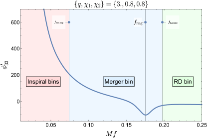
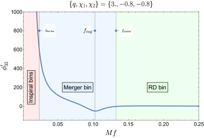
Figure 1: The phase derivative is shown for the $\ell=|m|=3$ spherical harmonic mode for two different configurations with high spins. The phase derivative changes rapidly in the inspiral region, and thus many grid points are required for accurate interpolation, the ringdown part is however comparatively flat, thus only few points are needed to describe it. The merger bin is characterized by the shape of the Lorentzian and determines the resolution required in this region.

II.1.1 Inspiral in the frequency domain

In order to derive an appropriate frequency grid spacing $\Delta f$ ($f$ is the dimensionless frequency in geometric units $G=c=1$) for the Fourier domain phase during inspiral, we will approximate the phase by the leading TaylorF2 phase expression Buonanno et al. (2009),

$$\Phi_{\ell m}=c_{0}+c_{1}f+\frac{m}{2}\frac{3}{128\eta}\left(\frac{2\pi f}{m}\right)^{-5/3},$$ (7)

where $\eta$ is the symmetric mass ratio, which in terms of the component masses $m_{1,2}$ of the binary reads $\eta=m_{1}m_{2}/(m_{1}+m_{2})^{2}$, and $c_{0}$, $c_{1}$ are constants of integration that do not affect the second derivative, which reads

$$\Phi^{\prime\prime}_{\ell m}=\frac{m}{2}\frac{5}{48\eta}\left(\frac{2\pi}{m}\right)^{-5/3}f^{-11/3}.$$ (8)

The phase and phase derivatives becomes singular as the frequency $f$ approaches zero, and the magnitude of the second derivative increases toward decreasing frequency. We can therefore estimate the maximal second phase derivative as the second derivative of the phase at the start of each frequency interval for which we want to use interpolation, assumed at frequency $f$, and obtain

$$\Delta f(f) = \sqrt{\frac{2R}{\Phi^{\prime\prime}(f)}}=\sqrt{\frac{2R}{c_{f,insp}}}f^{11/6},$$ (9)

$$c_{f,insp} = \frac{m}{2}\frac{5}{48\eta}\left(\frac{2\pi}{m}\right)^{-5/3}.$$ (10)

In Sec. II.3 we will use eq. (9) to split the calculation of the phase into frequency bins, where in each bin the grid spacing $\Delta f$ is kept constant, but it increases from bin to bin with increasing start frequency of the bin.

We now turn to the inspiral amplitude. For the modes we consider in this work we obtain the following leading order terms, see e.g. García Quirós et al. (2020), where we use the definitions $v=(2\pi f/m)^{1/3}$ and $\delta=\sqrt{1-4\eta}$:

$$A_{\ell m} = \pi\sqrt{2\eta/3}\,v^{-7/2}a_{\ell m},$$ (11)

$$a_{22} = 1+O(v^{2}),$$ (12)

$$a_{21} = v\delta\frac{\sqrt{2}}{3}+O(v^{2}),$$ (13)

$$a_{33} = v\delta\frac{3}{4}\sqrt{\frac{5}{7}}+O(v^{3}),$$ (14)

$$a_{32} = v^{2}\frac{1}{3}\sqrt{\frac{5}{7}}\,(1-3\eta)+O(v^{3}),$$ (15)

$$a_{44} = v^{2}\frac{4}{9}\sqrt{\frac{10}{7}}\,(1-3\eta)+O(v^{4}).$$ (16)

For the amplitude it is natural to define a threshold for the relative error of the interpolation, which we denote by $r$. The frequency dependent coarse grid resolution $\Delta f(f)$ which results from specifying a relative error threshold $r$ is then independent of $\eta$ and depends linearly on the frequency,

$$\Delta f_{\ell m}(f)=\sqrt{\frac{2rA_{lm}}{A_{lm}^{\prime\prime}}}=c_{\ell m}\,f\sqrt{r},$$ (17)

where

$$c_{22} = 6\sqrt{\frac{2}{91}},$$ (18)

$$c_{21} = c_{33}=6\sqrt{\frac{2}{55}},$$ (19)

$$c_{44} = c_{32}=2\sqrt{\frac{2}{3}}.$$ (20)

We can then write the ratio of coarse grid spacing required for the phase to stay below a phase error of $R$ radians to the coarse grid spacing required for the amplitude to guarantee a relative amplitude error below $r$ as

$$\frac{\Delta f_{phase}}{\Delta f_{amp}}=\alpha_{\ell m}\left(f\pi\right)^{5/6}\sqrt{\eta}\sqrt{\frac{R}{r}},$$ (21)

where

$$\alpha_{22} = 2\sqrt{\frac{91}{55}},\quad\alpha_{21}=2^{1/3}\sqrt{\frac{11}{3}},$$ (22)

$$\alpha_{33} = \frac{2^{7/3}}{3^{11/6}}\sqrt{11},\quad\alpha_{32}=\frac{6}{\sqrt{5}},\quad\alpha_{44}=\frac{3}{2^{1/3}\sqrt{5}}.$$ (23)

Choosing e.g. $r=R$ the expression (21) is always smaller than unity up to the minimum energy circular orbit (MECO) frequency Cabero et al. (2017), the step size restriction for the phase is thus more restrictive than the one for the amplitude. For simplicity we will use the phase criteria to build just one coarse frequency array and use this for both the phase and amplitude. We discuss the merger and ringdown in the next section.

II.1.2 Merger and ringdown in the frequency domain

The merger-ringdown phase exhibits a morphology that is rather different from the inspiral. A detailed phenomenological description for the $\ell=|m|=2$ is provided by the IMRPhenomD Husa et al. (2016) and IMRPhenomXAS Pratten et al. (2020) waveform models, and for subdominant modes by IMRPhenomXHM García Quirós et al. (2020). This allows us to identify the crucial features of the merger-ringdown regime, and to adapt the estimate (6) for the step size as we have done for the inspiral.

The first ingredient will be to identify the end of the inspiral. In Husa et al. (2020); Pratten et al. (2020); García Quirós et al. (2020) we confirm that the minimum energy circular orbit (MECO) Cabero et al. (2017) provides a good approximation for the transition between inspiral and merger for comparable masses. In the merger-ringdown part the Fourier domain phase derivative is given by a superposition of a Lorentzian function and a background term Pratten et al. (2020); García Quirós et al. (2020). The Lorentzian dominates the phase derivative and is given by (see eq. (6.3) in García Quirós et al. (2020)):

$$\Phi^{\prime}(f)=\frac{a}{\left(f-f_{0}\right)^{2}+b^{2}}$$ (24)

and the second derivative by

$$\Phi^{\prime\prime}(f)=-\frac{2a(f-f_{0})}{((f-f_{0})^{2}+b^{2})^{2}},$$ (25)

where we have introduced the shorthands $a=a_{\lambda}f_{\mathrm{damp}}^{lm}$, $b=f_{\mathrm{damp}}^{lm}$, and $f_{0}=f_{\mathrm{ring}}^{lm}$. Thus $\alpha_{\lambda}$ is a term that determines the overall amplitude of the Lorentzian, $f_{0}$ is the frequency at which the dip of the Lorentzian happens and $b$ is a measure of the ”width” of the dip. Inserting the expression for the Lorentzian into eq. (6) we obtain

$$\Delta f(f)=\sqrt{\frac{2R}{\Phi^{\prime\prime}(f)}}=\sqrt{\frac{R}{a|f-f_{0}|}}\left(\left(f-f_{0}\right)^{2}+b^{2}\right),$$ (26)

which replaces eq. (9) for computing the spacing of the coarse frequency grid in the merger and ringdown.

The spacing computed according to (6) depends on the absolute value of the second derivative, and we note that the second derivative of the Lorentzian phase function, $\Phi^{\prime\prime}$, has two local maxima for $f_{0}\pm b/\sqrt{3}$, with identical absolute value

$$\left|\Phi^{\prime\prime}\left(f_{0}\pm\frac{b}{\sqrt{3}}\right)\right|=\frac{3\sqrt{3}a}{8b^{3}}.$$ (27)

While for the inspiral the number of frequency bins depends on the start frequency, as we will discuss in more detail below in Sec. II.3, for the merger and ringdown we choose two bins which we call the merger and ringdown bins. The merger bin is defined by the frequency interval $\left(f_{\mathrm{Insp}},f_{\mathrm{Lorentzian}}\right)$, and captures the frequency regime where high resolution is required to capture the shape of the Lorentzian. The frequency $f_{\mathrm{Insp}}$ marks the end of the inspiral region of the IMRPhenomXAS model for the $\ell=|m|=2$ mode and the IMRPhenomXHM model for the other harmonics, and is chosen approximately at the MECO frequency (see Pratten et al. (2020) and García Quirós et al. (2020) for details). The frequency $f_{\mathrm{Lorentzian}}$ is defined as $f_{\mathrm{ring}}^{lm}+2f_{\mathrm{damp}}^{lm}$ and is chosen to approximate the lowest frequency where the second phase derivative of the Lorentzian can be neglected, and the first phase derivative is approximately constant. The ringdown bin starts at this frequency, and is the highest frequency bin in our procedure. It is characterized by low resolution requirements for the phase due to neglecting $\Phi^{\prime\prime}$ and ends at the end frequency of the waveform, the frequency range of this last bin is thus $\left(f_{\mathrm{Lorentzian}},f_{\mathrm{max}}\right)$.

We compute the grid spacing of both bins by evaluating the maximum value of $|\Phi^{\prime\prime}|$ in these two intervals according to eqs. (9, 27) and inserting it into eq. (6). For the merger bin this is the maximum of the inspiral value and the value for the Lorentzian, and thus

$$\Delta f_{\mathrm{merger}}^{phase}=\min{\left(\sqrt{\frac{2R}{c_{f,insp}}}f_{insp}^{\frac{11}{6}},\frac{4f_{\mathrm{damp}}^{lm}}{3^{3/4}}\sqrt{\frac{R}{|\alpha_{\lambda}|}}\right)},$$ (28)

For the ringdown bin the second phase derivative $|\Phi^{\prime\prime}|$ decreases monotonically to zero, we thus take the value at the start of the region $f_{\mathrm{Lorentzian}}$, which yields

$$\Delta f_{\mathrm{RD}}^{phase}=5\>f_{\mathrm{damp}}^{lm}\sqrt{\frac{R}{2|\alpha_{\lambda}|}}.$$ (29)

Again we turn to the amplitude now. We approximate the amplitude falloff in the ringdown bin as

$$h\approx e^{-\Lambda f},$$ (30)

with $\Lambda=\lambda/(f_{damp}^{lm}\sigma)$, where these coefficients correspond to those used in the ringdown ansatz for the IMRPhenomXHM model (see García Quirós et al. (2020) for more details):

$$A_{RD}^{\ell m}\propto\frac{1}{\left(f-f^{\ell m}_{ring}\right)^{2}+\left(f^{\ell m}_{damp}\>\sigma\right)^{2}}e^{-\frac{\left(f-f^{\ell m}_{ring}\right)\>\lambda}{f^{\ell m}_{damp}\sigma}}.$$ (31)

The grid spacing required to guarantee a relative error smaller than $r$ is then given by

$$\Delta f_{RD}^{amp}(r)=\frac{\sqrt{2\,r}}{\Lambda},$$ (32)

which is independent of the frequency $f$. For $r=R$ this condition is typically more restrictive than the condition (29) derived from the phase, the dependence across parameter space is however complicated. We therefore always compute the two frequency spacings, and then use the more restrictive one. We believe that this choice is quite conservative and that the choice could be relaxed in the future, since our ringdown bin only starts at frequencies where the amplitude is already quite small. Note that the start frequency of our ringdown region is either significantly higher than the ringdown frequency, or, for very high spins, the exponential falloff is significantly steeper than for moderate spins. In consequence we could use always the phase criterion (28) to set the grid spacing in the ringdown region without worrying too much about loss of accuracy. If greater amplitude accuracy for the ringdown would be required, it would be also possible to switch from linear interpolation to the fine grid to third order spline interpolation for the amplitude.

In the merger bin, the functional dependence of the mode amplitudes is more complex (see García Quirós et al. (2020)). In this case we compute numerically the grid spacing $\Delta f$ for the amplitude as

$$\Delta f_{merger}^{amp}=\sqrt{\frac{2\>r\>|h_{lm}(f)|}{|h_{lm}(f)|^{\prime\prime}}}.$$

We evaluate this quantity for the merger bin across our parameter space with the choice $r=R$ and compare with the grid spacing derived for the phase given by eq. (28). We find that the ratio $\Delta f_{merger}^{phase}/\Delta f_{merger}^{amp}$ is typically lower than one so the criteria for the phase is more restrictive than the one for the amplitude. We find that for some cases with comparable masses and high positive spins the ratio is between a value of one and two, but for simplicity we will always choose the criterion for the phase and interpret this choice such that the actual relative amplitude and phase errors will be bounded by the thresholds within a factor of four. We leave refinements of the simple strategy to set $r=R$ to future work. Below we will study the mismatch between the original model and different levels of error threshold to arrive at a more practical evaluation of error than to check for local deviations between model and approximation, and in Sec. III.3 we will perform a parameter estimation exercise and find that all choices of the value of $R=(0.1,0.01,0.001)$ lead to indistinguishable results for the case considered.

II.2 Efficient evaluation of complex exponentials

The evaluation of the complex exponential function when constructing the strain from amplitude and phase as in eq. (1) is one of the most time consuming operations in the C-code of the LALSuite The LIGO Scientific Collaboration (2015) implementation of our model. The number of required evaluations of the complex exponential (or, equivalently, of trigonometric functions), can however be reduced drastically by implementing the method described in Vinciguerra et al. (2017) (adapted from Press et al. (2007)). Instead of interpolating the phase on the uniform fine grid and computing the complex exponential, we compute the complex exponential in the non-uniform coarse grid and then rewrite the interpolation of this quantity in terms of an iterative algorithm.

Let $\Phi_{j}$ be the phase at one coarse frequency point $f_{j}$ and let $\hat{\Phi}_{k}$, $f_{k}$ be the estimated phase and the frequency at one point of the final uniform frequency grid, the spacing of the uniform grid is therefore $df=f_{k+1}-f_{k}$. Then we use the recursive property

$$e^{i\hat{\Phi}_{k+1}}=e^{i\hat{\Phi}_{k}}e^{i\>df\>\frac{\Phi_{j+1}-\Phi_{j}}{f_{j+1}-f_{j}}}.$$ (33)

This property is used to compute the complex exponential in the fine frequency grid points that lay between two coarse frequency points $j$ and $j+1$. The first of the fine points is given by $e^{i\hat{\Phi}_{0}}=e^{i\Phi_{j}}$.

II.3 Complete multibanding algorithm in the frequency domain

We will now describe our final algorithm for accelerated waveform evaluation, which is based on our previous results. Our final results will be the strain, evaluated on a uniform frequency grid, with a resolution $df$ that is adapted to the requirements of some given data analysis application. The motivation for uniform grid spacing stems for the typical context of matched filtering, where an inverse Fourier transform is used to optimize a match over the time shift between a signal and a template. We will refer to this uniform frequency grid as the fine grid. In order to accelerate the waveform evaluation we will however only evaluate our model waveform on a coarser non-uniform grid, and then use the iterative evaluation described above in Sec. II.2 to evaluate the complex exponential of the phase.

By default we will use linear interpolation for the amplitude, with optional cubic spline interpolation. Both interpolation algorithms are currently using the open source GSL library Galassi, Mark and Davies, Jim and Theiler, James and Gough, Brian and Jungman, Gerard and Alken, Patrick and Booth, Michael and Rossi, Fabrice and Ulerich, Rhys (2019), we do however expect a further speedup by replacing the GSL implementation by adding a standalone implementation of the required interpolations to our code.

We will now first discuss how to construct the non-uniform coarse frequency grid, and then the details of how to evaluate the waveform on the fine grid, first for spherical harmonics without mode mixing, and then for modes with mode mixing, which for the current IMRPhenomXHM models concerns only the $\ell=3,|m|=2$ mode.

II.3.1 Building the coarse frequency grid

We assume that we are given an input frequency range $(f_{min},f_{max})$ where we need to evaluate the spherical harmonic modes of the waveform. We wish to construct a non-uniform frequency grid, such that for every two successive frequency points the grid spacing $\Delta f(f)$ between them is sufficiently small to guarantee that the local phase error resulting from using linear interpolation between the coarse frequency points is smaller than a given threshold value $R$. We can then use eqs. (9, 26) to compute $\Delta f$ as a function of the threshold $R$, the frequency $f$, the intrinsic parameters $(q,\chi_{1},\chi_{2})$, and the spherical harmonic mode $(\ell,m)$ under consideration. The coarse grid will also depend on the desired grid spacing $df$ for the final uniform grid, since we build the coarse frequency grid such that the coarse points also belong to the fine grid. This simplifies the interpolation procedure for the complex exponential.

Lower values for the threshold $R$ result in smaller errors, but higher computational cost. In Sec. III we will compare different threshold settings and evaluate the computational cost and compare the actual errors with the chosen threshold $R$.

As mentioned above in Sec. II.1 we split the frequency range into three regions corresponding to the inspiral, merger and ringdown. For the practical implementation, instead of using the continuously varying $\Delta f(f)$ of expressions (9, 26), we work with a series of frequency bins where $\Delta f$ is fixed in each bin. The merger and ringdown parts have a much smaller dynamic range for $\phi^{\prime}(f)$ than the inspiral part (the phase “flattens out” from inspiral toward merger), and we just use one frequency bin for each region. Their spacings $\Delta f_{\mathrm{merger}}$ and $\Delta f_{\mathrm{RD}}$ are given by eqs. (28) and (29-32) respectively.

However, the inspiral part has a large dynamic range, and $\Delta f$ given by (9) changes with a power law of $f^{11/6}$ so it also changes fast. The spacing that would accurately describe the whole inspiral part would be $\Delta f(f_{\mathrm{min}})$, however if we used this spacing for the whole region, we would be using many more points than what are really needed since $\Delta f$ increases so much for frequencies above $f_{\mathrm{min}}$. Therefore we use a varying number of frequency bins $N$, and we build each of them with a spacing $\Delta f_{i}$ twice larger than the previous bin. For the first bin we set $\Delta f_{0}=\Delta f(f_{\mathrm{min}})$, thus

$$\Delta f_{0} =\sqrt{\frac{2R}{c_{insp}}}f_{min}^{11/6}$$ (34)

$$\Delta f_{i} =2^{i}\>\Delta f_{0},\hskip 28.45274pti=1,2,...,N.$$ (35)

In practice we require that between two coarse points there is an integer number of fine frequency points, in consequence we modify $\Delta f_{0}$ such that

$$\Delta f_{0}^{\prime}=\texttt{int}\left[\frac{\Delta f_{0}}{df}\right]\>df.$$ (36)

Now that we have computed the spacing of each frequency bin, we need to compute the final frequency of each bin $f_{i,\mathrm{end}}$, which is the frequency that doubles the spacing $\Delta f$ of the current bin, i.e. we have to solve the equation $\Delta f(f_{i,\mathrm{end}})=2\>\Delta f_{i}$. Inserting this into eq. (9) we obtain

$$f_{i,\mathrm{end}}^{\frac{11}{6}} =2\>f_{i,\mathrm{start}}^{\frac{11}{6}},$$ (37)

$$\frac{f_{i,\mathrm{end}}}{f_{i,\mathrm{start}}} =2^{\frac{6}{11}}.$$ (38)

We require that in a frequency bin there must be an integer number of coarse frequency points, and so we modify the end frequencies of each bin to

$$f_{i,\mathrm{end}}^{\prime}=\texttt{int}\left[\frac{f_{i,\mathrm{end}}-f_{i,\mathrm{start}}}{\Delta f_{i}}\right]\Delta f_{i}.$$ (39)

With the above frequency factor we can estimate the number $N$ of bins that will be used in the inspiral. Since the inspiral regions ends at $f_{\mathrm{insp}}$, $N$ has to satisfy the relation

$$\frac{f_{\mathrm{insp}}}{f_{\mathrm{min}}}=\left(2^{\frac{6}{11}}\right)^{N},$$ (40)

and therefore we obtain

$$N=\log_{2^{\frac{11}{6}}}\left(\frac{f_{\mathrm{insp}}}{f_{\mathrm{min}}}\right).$$ (41)

Since $N$ is however the number of constant frequency bins for the inspiral, it has to be an integer, and we modify $f_{\mathrm{insp}}$ such that

$$N=\log_{2^{\frac{11}{6}}}\left(\frac{f_{\mathrm{insp}}^{\prime}}{f_{\mathrm{min}}}\right)=\texttt{int}\left[{\log_{2^{\frac{11}{6}}}\left(\frac{f_{\mathrm{insp}}}{f_{\mathrm{min}}}\right)}\right].$$ (42)

For the merger and ringdown regions, we proceed analogously to the inspiral region, and ensure that an integer number of fine grid points aligns with the coarse grid. Since this algorithm depends on the input values for $f_{min}$, $f_{max}$ and $df$, we perform several sanity checks to ensure that there is not any overlapping between regions. For example, if $f_{\mathrm{insp}}>f_{\mathrm{Lorentzian}}$ we skip the merger bin or if $f_{\mathrm{Lorentzian}}>f_{max}$ we skip the ringdown bin.

In Fig. 2 we compare the final non-uniform coarse grid with the uniform grid. In the top panel we can see how the frequency spacing $\Delta f$ increases for subsequent bins that constitute the inspiral part. In the case shown the merger bin has a slightly lower $\Delta f$ than the last inspiral bin in order to resolve the Lorentzian feature of the phase derivative. For other cases where the Lorentzian is less pronounced the limiting factor will be the derivative at the end of the inspiral and then the merger will have exactly twice the spacing of the last inspiral bin. The ringdown bin is the one with a coarser $\Delta f$ since there the phase derivative is practically flat. In the bottom panel we show the number of frequency points for the inspiral, merger and ringdown parts. The uniform grid has most of its frequency points in the merger-ringdown part, which leads to an excessive computational cost in these regions, where far fewer points are required to capute the flatter behaviour of the phase derivative (see Fig. 1). For the non-uniform grid most of the points are located in the inspiral part, where high resolution is needed to describe the phase derivative.

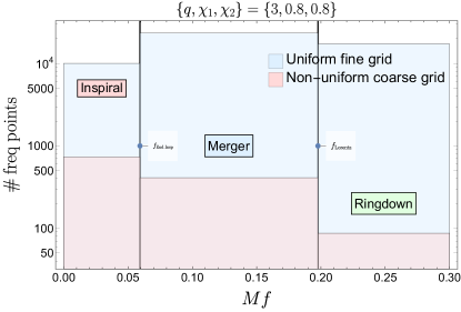
Figure 2: Comparison between uniform fine frequency grid and non-uniform coarse grid for the 33 mode for a high spin case. Top panel: The frequency spacing is shown for each frequency bin as a function of frequency. In the merger bin $\Delta f$ is smaller than the last one of the inspiral due to the need of resolving the dip of the Lorentzian. Bottom panel: The number of frequency points is shown for each frequency region. In a uniform grid most of the points lie in the merger and ringdown part where they are not so necessary, however this is corrected in the non-uniform grid.

Now that we have described the non-uniform coarse frequency grid, the next step is to evaluate the model in this grid and carry out the interpolation to the fine grid. In this next step however, different procedures need to set up follow for the modes with and without mixing, as we discuss below.

II.3.2 Evaluate the modes on the fine grid, with and without mode-mixing

For the modes without mixing (at the moment all modes except $\ell=3,|m|=2$), the waveform modes are evaluated on the fine grid as follows:

1. First the amplitude and phase are evaluated separately for the coarse frequency grid, which yields two 1D arrays, one for the amplitude and one for the phase.

2. The complex exponential $e^{i\phi}$ is computed on the coarse grid.

3. The fine uniform frequency grid is constructed with spacing $df$.

4. The complex exponential is interpolated to the final uniform frequency grid following the procedure described in Sec. II.2.

5. The amplitude is interpolated to the fine grid by using linear (optionaly third) order interpolation (using the GSL library).

6. The complex waveform $\tilde{h}_{lm}$ is constructed by multiplying the arrays for the amplitude and the complex exponential on the fine grid.

For the modes with mixing (in our present implementation of IMRPhenomXHM this is only the $\ell=3,|m|=2$ mode) our procedure is slightly different from the modes without mixing. To handle mode-mixing, in the ringdown region the model is built in terms of spheroidal harmonics instead of spherical harmonics, to simplify the waveform and avoid sharp features in the phase derivative and in the amplitude, as discussed in detail in García Quirós et al. (2020). After building the model waveform in terms of spheroidal harmonics, it is then rotated back to spherical harmonics and connected with the inspiral part, which is directly modelled in terms of spherical harmonics. Performing our interpolation in terms of the spherical harmonics as for the other modes would require significantly higher resolution and increase computational cost. We thus use the same strategy as we have employed to construct the original model, and apply our multibanding algorithm separately to the inspiral region expressed in spherical harmonics, and to the ringdown part expressed in spheroidal harmonics, and then transform the latter to spherical harmonics once the fine grid values have been computed. Our detailed procedure is as follows:

1. We split the coarse frequency array into the spherical part, where we will perform the model evaluation and multibanding in terms of the spherical harmonics, and the spheroidal part, where we transform from the spheroidal to the spherical representation in the ringdown region.

   The start frequencies of the ringdown region for the phase and amplitude, $f_{RD}^{\mathrm{phase}},f_{RD}^{\mathrm{amp}}$, are given in eq. (5.2) in García Quirós et al. (2020). Note that $f_{RD}^{\mathrm{phase}}<f_{RD}^{\mathrm{amp}}$. For our multibanding algorithm we split between the “spherical” and “spheroidal” coarse grids, where the spherical and spheroidal amplitude and phase are computed. There is some overlap between the frequency ranges of both in the interval ($f_{RD}^{\mathrm{phase}}$, $f_{RD}^{\mathrm{amp}}$), since the spherical array goes up to $f_{RD}^{\mathrm{amp}}$, but the spheroidal one starts at $f_{RD}^{\mathrm{phase}}$, see step (8) below.

2. Evaluate the spherical amplitude and phase in the spherical coarse array and evaluate the spheroidal amplitude and phase in the spheroidal coarse array, we get therefore four one-dimensional arrays.

3. Compute the complex exponential for the two coarse arrays of phases.

4. Build the uniform frequency grid with spacing $df$ and split into spherical and spheroidal parts as above.

5. Interpolate the two arrays of complex exponential in their respective regions using the iterative procedure described in II.2.

6. Interpolate the two arrays of amplitude in their respective regions using linear (optionally third) order splin interpolation using the GSL library Galassi, Mark and Davies, Jim and Theiler, James and Gough, Brian and Jungman, Gerard and Alken, Patrick and Booth, Michael and Rossi, Fabrice and Ulerich, Rhys (2019).

7. We have thus obtained four arrays: spherical amplitude and complex exponential evaluated in the spherical fine grid, and spheroidal amplitude and complex exponential in the spheroidal fine grid.

8. Finally we combine amplitude and phase with different procedures in three frequency ranges:

   • $f_{min}\leq f<f_{RD}^{\mathrm{phase}}$: We directly multiply spherical harmonic amplitude and complex exponential.

   • $f_{RD}^{\mathrm{phase}}\leq f<f_{RD}^{\mathrm{amp}}$: We rotate to spherical the spheroidal complex exponential term (which requires the spheroidal amplitude), and then multiply the resulting spherical complex exponential with the spherical amplitude.

   • $f_{RD}^{\mathrm{amp}}<f\leq f_{max}$: We first multiply the spheroidal amplitude and complex exponential and then transform to the spherical basis.

III Results

III.1 Computational performance

In first place we test the gain in speed due to multibanding and compare the results for different threshold values and for different spacings of the fine frequency grid. Note that the frequency spacing $df$ of the grid in the Fourier domain is related to the duration $T$ of the time segment that is analyzed by

$$df=\frac{1}{T},$$ (43)

and thus longer signals require a smaller grid spacing. To illustrate this dependency, in Fig. 3 we show the approximate duration of a binary black hole coalescence signal as a function of mass and mass ratio. To leading post-Newtonian order the duration in dimensionless units is given by

$$T/M=\frac{5}{256\eta\,(\pi Mf_{0})^{8/3}},$$ (44)

where $f_{0}$ is the frequency where the dominant spherical harmonic mode, $|\ell=|m|=2$ enters the frequency band of the detector. Lower start frequencies thus imply much longer signals. In Fig. 3 we show results for two values of the lower frequency cutoff of the detector, $f_{0}=$ 10 Hz, 20 Hz, the latter is what is typical for current compact binary parameter estimation, see e.g. Abbott et al. (2016); Chatziioannou et al. (2019). The coalescence time is approximated with the TaylorT2 approximant at second post-Newtonian order spins aligned with the orbital angular momentum, and extreme Kerr values, adding a time of $500M$ in geometric units to account for merger and ringdown, in order to obtain an approximate upper limit on the duration. The figures focus on short signals, where time duration of 4 seconds is appropriate, and show the range of signals and templates in mass and mass ratio that fit into this time window.

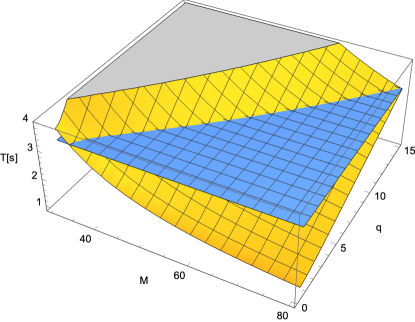
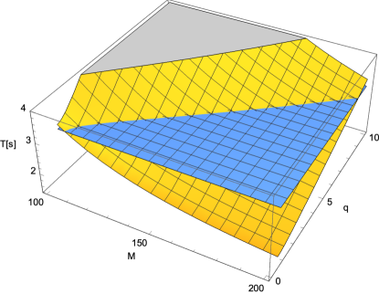
Figure 3: The approximate merger time observed by a detector with lower frequency cutoff at 20 Hz (upper panel) and 10 Hz (lower panel) is shown as a function of the total mass and the mass ratio of the system. The blue horizontal surface marks a duration of three seconds, which would allow for one second of buffer time between the signal duration and the length of the data segment. For a start frequency of 10 Hz only very high mass signals fit the time window.

We will now discuss an example case of a non-spinning system of black holes with total mass of $50$ solar masses and mass ratio $m_{1}/m_{2}=1.5$, and evaluate the computational cost as a function of frequency spacing $df$. In Fig. 4 we show the evaluation time of one waveform versus the spacing of the final uniform frequency grid. The frequency range spans from 10 to 4096 Hz and we fix the mass of the system to 50 $\mathrm{M}_{\odot}$. The dashed lines represent the waveforms generated without multibanding while the solid lines correspond to the multibanding version with different values of the threshold: $10^{-1}$, $10^{-2}$, $10^{-3}$ and $10^{-4}$. First, we focus on the no-multibanding results, in principle we would expect that the higher modes model is 5 times slower than the 22-mode-only model because IMRPhenomXHM has 5 modes instead of just one. However it is a bit more expensive due to some particularities that are only present in the higher modes code, like the checks for the amplitude veto and mainly the extra steps needed to describe the mode-mixing of the 32 mode.

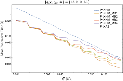
Figure 4: Evaluation time of the LAL code for waveforms with and without multibanding (solid and dashed lines respectively) for a total mass of 50 $M_{\odot}$. PhXAS denotes the quadrupole model, and the different “PhXHM_MB” items in the legend correspond to different values of the threshold $R$: $10^{-1}$, $10^{-2}$, $10^{-3}$ and $10^{-4}$. The evaluation time is averaged over 100 repetitions. The results are shown as a function of the spacing of the fine uniform frequency grid $df$. They were obtained with the LIGO cluster CIT.

Focusing now on the results with multibanding, notice that when $df$ is coarser the multibanding tends to equalize the no-multibanding. This is expected since for coarser $df$ we have less frequency points and then the coarse and fine grid tends to be similar and there is no gain by using the interpolation. Also it happens that the input $df$ may be larger than the $\Delta f$ of the coarse grid given by the multibanding criteria, in these cases we just evaluate in the frequency points of the fine grid and there is no gain in speed. In current LIGO-Virgo parameter estimation the highest $df$ that is used is 0.25 Hz, since $df$ is the inverse of the time duration of the signal as in eq. (43), and in practice the smallest duration considered, e.g. for high mass events with very short duration, is four seconds. Note however that as low frequency noise is reduced in detectors, and the lower cutoff frequency for data analysis can be lowered, waveforms get longer and frequency spacings are reduced.

On the contrary, when $df$ is very small we have a lot of points in the fine grid, then the interpolation is much more efficient and the multibanding has the highest gain in speed.

The different values of the threshold behave as expected: larger values of the threshold are less accurate, but allow faster evaluation. For small $df$ we observe however that the evaluation speed is almost independent of the threshold value. This is due to the fact that for small $df$ the evaluation of the model at the coarse grid points is computationally much cheaper than the subsequent interpolation to the fine grid points. Future optimization of our code will be required to address this issue and intend to reduce the computational cost of the interpolation to the fine grid.

We now show the dependence of the evaluation time on the total mass of the system. In this case the spacing of the fine grid $df$ is computed by the LAL function XLALSimInspiralFD which adapts the $df$ accordingly to an internal estimation of the time duration of the signal which depend on the lower cutoff $f_{min}$, chosen here as $f_{min}=10Hz$, and the mass of the system. This is similar in spirit to the estimate of the merger time that we have used in Fig. 3. In Fig. 5 we see qualitatively the same results than when simply scaling $df$ as in Fig. 4. The multibanding is more efficient for lower masses where the duration of the signal is lower and therefore a smaller $df$ is used.

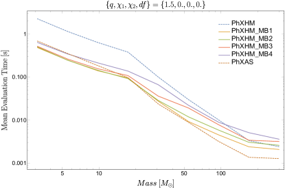
Figure 5: Evaluation time versus total mass of the system, choosing a fine grid spacing $df$ that corresponds approximately to the inverse merger time at this mass ratio, as is common on data analysis applications (we denote this behaviour by writing $df=0$). The evaluation time is averaged over 100 repetitions. Result were obtained with the LIGO cluster CIT.

III.2 Accuracy

In this section we discuss the accuracy of the multibanding algorithm as well as compare different choices of the threshold and motivate the choice of the default value for the model. In section  II.1 we explained that the non-uniform coarse grid is built such that the error in the phase (of a single mode) is below a threshold $R$. To check this we compute the waveform with and without multibanding for 150000 random configurations in the parameter range $M_{tot}\in[1,500]M_{\odot}$, $q\in[1,1000]$, $\chi_{1,2}\in[-1,1]$, and $df\in[0.01,0.25]$Hz. For the multibanding we compare again four different threshold values. In Fig. 6, we first show the maximum absolute error for the whole uniform frequency array for all the modes except $\ell=3,m=2$, where mode mixing needs to be taken into account for interpreting results as discussed below. We see that for most cases the maximum error is indeed below the threshold. However there can be special configurations where a few frequency points may give an error above the threshold. These few cases correspond typically to configurations where the approximations employed by the algorithm are less accurate, e.g. using the TaylorF2 phase to approximate the phase in the inspiral to compute $\Delta f$ for extreme spins or for cases with high mass, where the inspiral starts at high frequencies where the TaylorF2 is again less accurate. In Fig. 7 we show the mean error, averaged over the frequency array, always remains below the thresholds. We will also compute mismatches between the original and the interpolated below, and find that we indeed achieve acceptably low values of the mismatch, see Fig. 10.

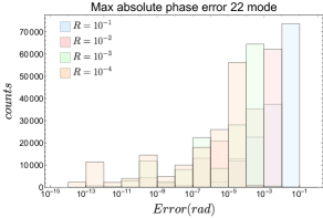
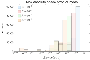
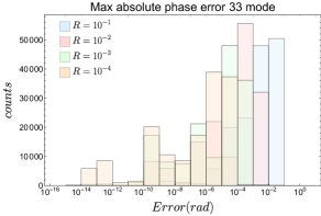
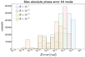
Figure 6: Maximum absolute error for the phase of the $(l,m)$ mode between the multibanding and no-multibanding waveforms for four values of the threshold $R$. The threshold $R$ can be interpreted as an approximate upper limit for the maximum absolute error introduced in the phase.

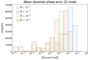
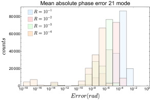
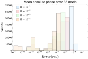
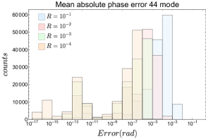
Figure 7: Absolute error for the phase averaged over the frequency array for the $(l,m)$ modes between the multibanding and no-multibanding waveforms for four values of the threshold $R$. The threshold $R$ can be interpreted as an approximate upper limit for the absolute error introduced in the phase.

Now we consider the 32 mode, where mode mixing with the 22 mode is present. In Fig. 8 we show the results for the same test as shown in Fig. 6 for the other modes. The interpretation of the results is however different now, since the ringdown of the 32 mode, where mode mixing is present, is modelled and interpolated in terms of the spheroidal harmonics, see García Quirós et al. (2020), where the waveform phenomenology is much simpler than in terms of spherical harmonics.

In Fig. 9 we show some typical behaviour for mode mixing in the ringdown: Here the complex waveform comes very close to or crosses zero, visible as a sharp feature in the logarithm of the amplitude. Near the zero-crossing splitting the waveform into a spherical harmonic amplitude and phase creates artefacts when computing phase differences or relative amplitude errors between two waveforms, even if they are very close. Comparing our theoretical thresholds with the phase only makes sense in the spheroidal basis, but not in the spherical one. We omit a comparison of the phase errors in the ringdown as computed in the spheroidal picture in order to avoid excess baggage in our LALSuite implementation. We thus arrive at the following interpretation of Fig. 8: while phase errors are typically small and below the threshold, a significant number of outliers arise due to the phenomenon shown in Fig. 9, they are however not due to problems of the multibanding algorithm, but due to keeping our test simple and uniformly comparing in the spherical harmonic picture for all modes and across the whole frequency range.

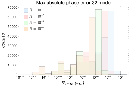
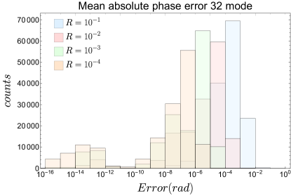
Figure 8: Maximum absolute error (top) and averaged over the frequency array (bottom) for the phase of the $(3,2)$ mode between the multibanding and no-multibanding waveforms for four values of the threshold $R$.

Figure 9: Example case that produces a maximum phase error above the threshold for the 32 mode. The parameters for this case are $m_{1}=35.7M_{\odot}$, $m_{2}=16.6M_{\odot}$, $\chi_{1}=0.33$, $\chi_{2}=-0.54$. Top panel: Absolute phase error between the no-multibanding and multibanding waveform with $R=0.1$ versus the frequency. Bottom panel: amplitude of the 32 mode for the no-multibanding and multibanding. Notice the correspondence of the maximum phase error with the deep in the amplitude of the 32 mode.

To truly understand the accuracy of the algorithm we have to compute the mismatch between the two waveforms. In the following we evaluate the multimode waveform and compute the mismatch for the $h_{+}$ polarization. We carry out an extensive study across the whole parameter space also to test the robustness of the algorithm and evaluate one million of random configurations in the parameter space. The results are shown in Fig. 10. As expected the threshold $10^{-4}$ has the lowest mismatches since it is the most accurate and the threshold $0.1$ has the worst mismatches because it is the less accurate. The reader may be wondering why there are a significant number of cases with mismatch $10^{-16}$ since we would expect that the number of cases decreases with the higher accuracy. The explanation is that in this bin the randomly chosen $df$ is coarser than the $\Delta f$ that the multibanding criteria provides, and in this case we replace $\Delta f$ with $df$ and in consequence there is no difference between the multibanding and no-multibanding and we reach matching precision.

Fig. 10 is also very useful to decide which threshold we want to use as default value in the LAL code. We consider that $R=10^{-3}$ performs well in accuracy and given that is faster than the $10^{-4}$ we set this as the default value.

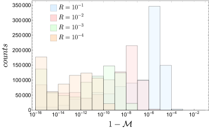
Figure 10: Mismatches between the no-multibanding and multibanding waveforms for one million random configurations across parameter space. We show the results for four different values of threshold. The configurations are choosen randomly with $q\in[1,1000]$, $\chi_{1,2}\in[-1,1]$, $\mathrm{M_{t}}\in[1,500]M_{\odot}$, $df\in[0.01,0.3]$ Hz, $\iota\in[0,\pi]$, $f_{min}=10Hz$, $f_{max}=1024Hz$. The mismatch is computed for the $h_{+}$ polarization.

III.3 Parameter Estimation

In order to illustrate our algorithm in a parameter estimation application, we compare the performance of the original model and different choices for the threshold parameter $R$.

We select a publicly available numerical relativity data set from the SXS waveform catalogue SXS , SXS:BBH:0264, which corresponds to a binary black hole merger at mass ratio 3, with individual spins of $-0.6$ anti-aligned with the orbital momentum. Then we inject this numerical relativity simulation into zero noise as a way to get a non-precessing and non-eccentric strain of 4 seconds of duration, with $100~{}M_{\odot}$ total mass, near edge on with $\pi/3$ rad of inclination. We use a relatively close source at 430 Mpc, which implies a signal-to-noise ratio of 28. Recovery of the signal uses the advanced LIGO zero detuning high power noise curve LIG . We choose the parameters in order to challenge our approximations in the regime where higher modes are particularly relevant, not in order to demonstrate significant computational gains, which by Fig. 3 when the lower cutoff frequency of the detector sensitivity would be lower than the 20 Hz we have chosen here to compute the likelihood function in our Bayesian inference algorithm (see e.g. Veitch et al. (2015); Ashton et al. (2019) for details of Bayesian inference for compact binary coalescence signals). Note that the start frequency of the numerical relativity waveform we choose here is approximately 9 Hz at $M=100M_{\odot}$.

For our analysis we use a sampling method called “Nested Sampling” Skilling (2006), in particular the CPNest sampler Veitch and Pozzo (2017) as implemented in the Python-based Bayesian inference framework Bilby Ashton et al. (2019). For each waveform model used, we carry out runs with five different seeds and 2048 “live points” in the language of nested sampling, and we merge the results from the five seeds to a single posterior result.

We define prior distributions as follows: The mass ratio is assumed to be uniform between $0.125$ and $1$, and the chirp mass prior is assumed uniform between 15 and $60~{}M_{\odot}$. The luminosity distance is uniform in volume with a maximal allowed distance at 1500 MPc. Finally, the magnitudes of the dimensionless black hole spins are uniform with an upper limit at $0.99$.

Our main results concern the comparison of the IMRPhenomXHM model, evaluated with different values of the threshold parameter, $R=(10^{-1},~{}10^{-2},~{}10^{-3})$ as well as without multibanding, which corresponds to $R=0$. The IMRPhenomXHM model includes the spherical harmonic modes $(l,\left|m\right|)=(2,2),(2,1),(3,2),(3,3),(4,4)$. Differences between the recovered value of parameters and the injected parameters may arise due to the approximations in our multibanding algorithm, errors in the IMRPhenomXHM model, errors in the numerical relativity waveform, and the absence of modes in the model, which are present in the numerical relativity data set (which contains all modes up to $l=8$). We also compare with the IMRPhenomXAS model, which corresponds to IMRPhenomXHM with only the $(l,\left|m\right|)=(2,2)$ modes and no multibanding. The latter serves as a comparison in terms of the errors in recovering the injection parameters.

Our results are presented in Fig. 11. In the case of the higher modes model, the injected values are recovered by the most probable regions of the posterior distributions. However, for the dominant mode model, a significant bias in the recovered parameters can be observed. This confirms the importance of the higher mode contributions for the case we have chosen. All the results for IMRPhenomXHM are consistent within the statistical errors implied by our finite sampling. As expected, in the case presented here the sampling time only decreases weakly when increasing the threshold value. We attribute the observed parameter bias for IMRPhenomXHM to the incomplete set of modes described by the model, as well as modelling errors. Future work will investigate the effect of dropping modes in the model in more detail.

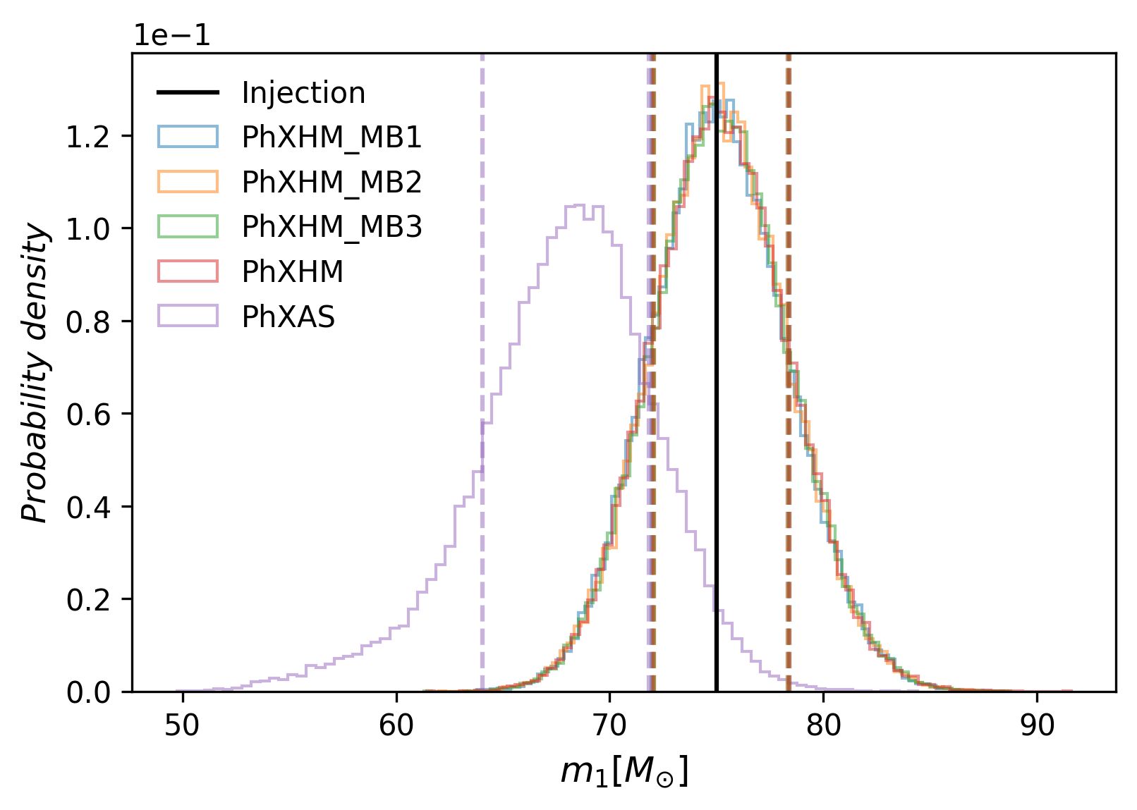
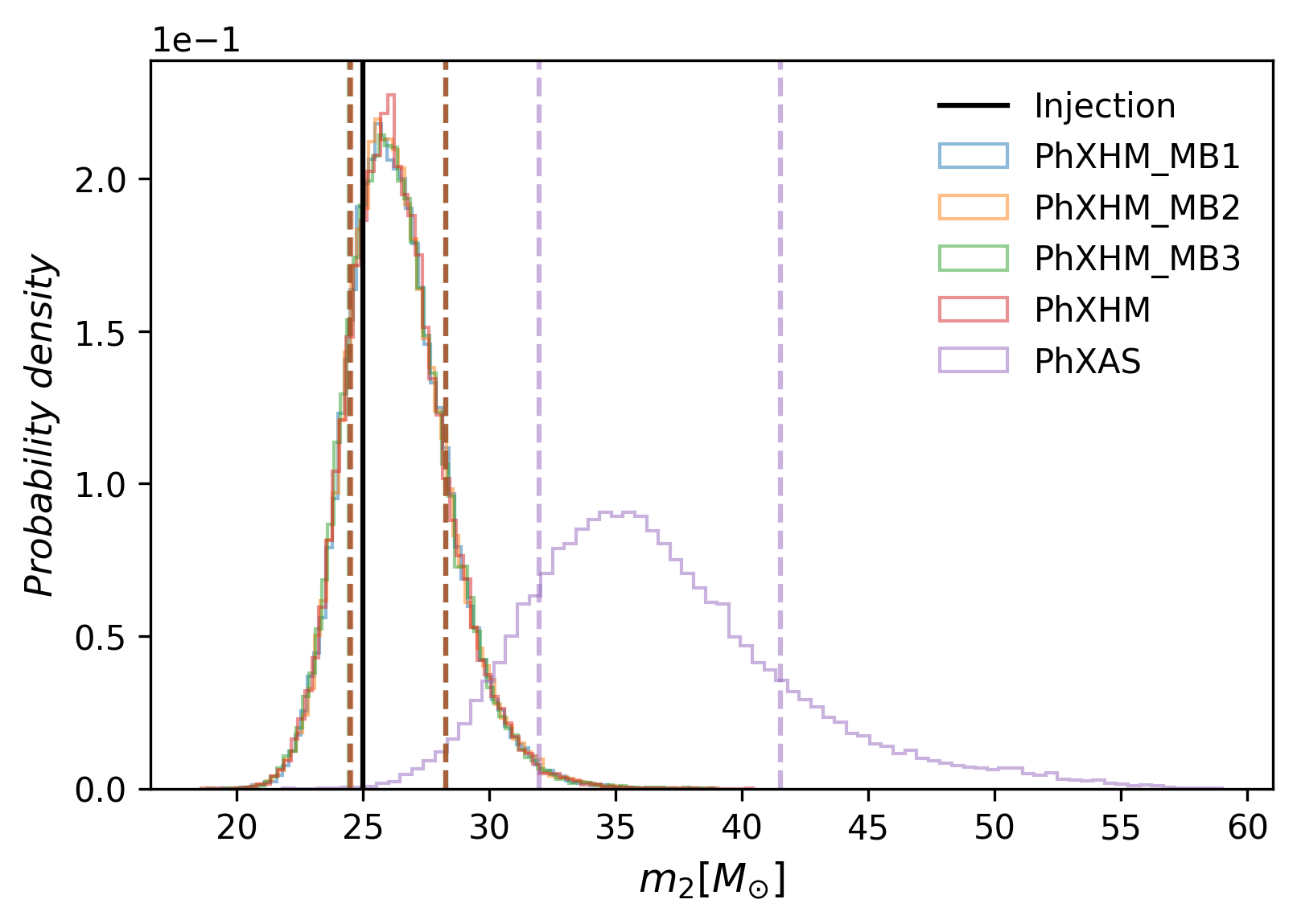
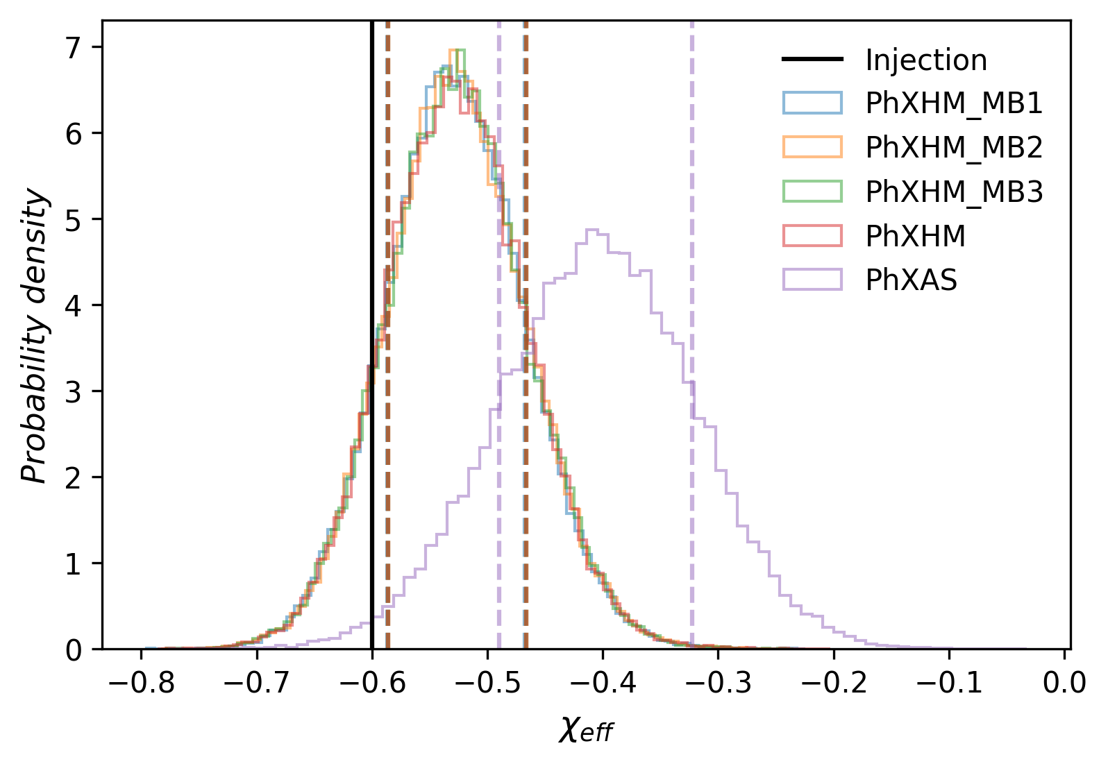
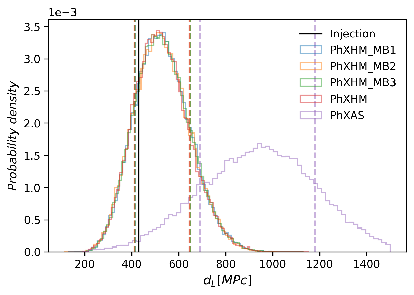
Figure 11: Posterior distributions of component masses, effective aligned spin and inclination respectively using waveforms with multibanding (PhXHM_MB) for different values of threshold ($10^{-1}$, $10^{-2}$, $10^{-3}$) and without it (PhXHM and PhXAS). The dashed vertical lines mark the $90\%$ confidence limits.

IV Conclusions

We have presented a simple way to accelerate the evaluation of frequency domain waveforms by first evaluating on a coarse grid, and then interpolating to a fine grid with an iterative scheme to evaluate complex exponential functions (or equivalently trigonometric functions). This works builds upon the method presented in Vinciguerra et al. (2017), but represents the heuristic criterion used there to determine the spacing of the coarse grid by the standard estimate for first order interpolation error, and then extends the criterion for the coarse frequency spacing to the merger and ringdown. Several extensions of our algorithm are possible: First, similar techniques can also be developed for the time domain. The simple estimates to determine the appropriate coarse grid spacing given a threshold parameter could be improved, e.g. by adding low order spin terms. The amplitude could be treated in a similarly careful way as the phase.

Acceleration is more significant for smaller spacings of the fine grid, as is appropriate for smaller masses, and for detectors with broader sensitivity in frequency, e.g. future detectors such as the upgrades of the current generation of the advanced detector network, the Einstein Telescope Punturo et al. (2010) or LISA Amaro-Seoane et al. (2017). For total masses around three solar masses, as is appropriate for binary neutron star masses, the current speed of the multi-mode IMRPhenomXHM roughly equals the speed of IMRPhenomXAS for the $\ell=|m|$ modes. Detailed profiling of the code reveals this rough equality as a coincidence, and performance is limited by a small number of bottlenecks, e.g. evaluating the spline interpolation for the amplitude, for which we use the GSL library Galassi, Mark and Davies, Jim and Theiler, James and Gough, Brian and Jungman, Gerard and Alken, Patrick and Booth, Michael and Rossi, Fabrice and Ulerich, Rhys (2019). Future optimization work will focus on these bottlenecks. Another possible avenue for further speedup would be an implementation on GPUs or similar highly parallel hardware.

The availability of a threshold parameter that regulates accuracy and speed also allows future applications to tune codes for parameter estimation, where the threshold parameter could be set depending on the information associated with the detection in a search (such as the signals rough parameter estimate from the search and its signal-to-noise ratio), or the threshold could be changed dynamically, and could be relaxed in the burn-in-phase of a parameter estimation simulation, or in the early stages of a nested sampling run. The coupling of strategies to accelerate the evaluation of individual waveforms evaluation and Bayesian parameter estimation simulations as a whole may also have implications on the development of future waveform models, which could introduce further parameters to tune accuracy and evaluation speed.

References

- Vinciguerra et al. (2017) S. Vinciguerra, J. Veitch, and I. Mandel, Class. Quant. Grav. 34, 115006 (2017), eprint 1703.02062.
- The LIGO Scientific Collaboration (2015) The LIGO Scientific Collaboration, LALSuite: LSC Algorithm Library Suite, https://www.lsc-group.phys.uwm.edu/daswg/projects/lalsuite.html (2015).
- García Quirós et al. (2020) C. García Quirós, M. Colleoni, H. Estellés, G. Pratten, A. Ramos-Buades, M. Mateu, and R. Jaume (2020).
- Abbott (2016) B. P. e. a. Abbott (LIGO Scientific Collaboration and Virgo Collaboration), Phys. Rev. Lett. 116, 061102 (2016), URL https://link.aps.org/doi/10.1103/PhysRevLett.116.061102.
- Abbott (2017) B. P. e. a. Abbott (LIGO Scientific Collaboration and Virgo Collaboration), Phys. Rev. Lett. 119, 161101 (2017), URL https://link.aps.org/doi/10.1103/PhysRevLett.119.161101.
- Abbott et al. (2018) B. P. Abbott et al. (LIGO Scientific, Virgo) (2018), eprint 1811.12907.
- Taracchini et al. (2014) A. Taracchini, A. Buonanno, G. Khanna, and S. A. Hughes, Phys. Rev. D90, 084025 (2014), eprint 1404.1819.
- Bohé et al. (2017) A. Bohé et al., Phys. Rev. D95, 044028 (2017), eprint 1611.03703.
- Ajith et al. (2007) P. Ajith, S. Babak, Y. Chen, M. Hewitson, B. Krishnan, J. T. Whelan, B. Brügmann, P. Diener, J. Gonzalez, M. Hannam, et al., Class. Quantum Grav. 24, S689 (2007), ISSN 1361-6382, URL http://dx.doi.org/10.1088/0264-9381/24/19/S31.
- Ajith et al. (2011) P. Ajith, M. Hannam, S. Husa, Y. Chen, B. Brügmann, N. Dorband, D. Müller, F. Ohme, D. Pollney, C. Reisswig, et al., Physical Review Letters 106 (2011), ISSN 1079-7114, URL http://dx.doi.org/10.1103/PhysRevLett.106.241101.
- Hannam et al. (2014) M. Hannam, P. Schmidt, A. Bohé, L. Haegel, S. Husa, et al., Phys.Rev.Lett. 113, 151101 (2014), eprint 1308.3271.
- Husa et al. (2016) S. Husa, S. Khan, M. Hannam, M. Pürrer, F. Ohme, X. Jiménez Forteza, and A. Bohé, Phys. Rev. D93, 044006 (2016), eprint 1508.07250.
- Khan et al. (2016) S. Khan, S. Husa, M. Hannam, F. Ohme, M. Pürrer, X. Jiménez Forteza, and A. Bohé, Phys. Rev. D93, 044007 (2016), eprint 1508.07253.
- Blackman et al. (2015) J. Blackman, S. E. Field, C. R. Galley, B. Szilagyi, M. A. Scheel, et al. (2015), eprint 1502.07758.
- Blanchet (2014) L. Blanchet, Living Reviews in Relativity 17 (2014), ISSN 1433-8351, URL http://dx.doi.org/10.12942/lrr-2014-2.
- Kokkotas and Schmidt (1999) K. Kokkotas and B. Schmidt, Living Reviews in Relativity 2 (1999), ISSN 1433-8351, URL https://doi.org/10.12942/lrr-1999-2.
- Barack and Pound (2019) L. Barack and A. Pound, Rept. Prog. Phys. 82, 016904 (2019), eprint 1805.10385.
- Buonanno and Damour (1999a) A. Buonanno and T. Damour, Phys. Rev. D59, 084006 (1999a), eprint gr-qc/9811091.
- Buonanno and Damour (1999b) A. Buonanno and T. Damour, Phys. Rev. D 59 (1999b), ISSN 1089-4918, URL http://dx.doi.org/10.1103/PhysRevD.59.084006.
- Klimenko et al. (2016) S. Klimenko et al., Phys. Rev. D93, 042004 (2016), eprint 1511.05999.
- Usman et al. (2016) S. A. Usman et al., Class. Quant. Grav. 33, 215004 (2016), eprint 1508.02357.
- Sachdev et al. (2019) S. Sachdev et al. (2019), eprint 1901.08580.
- Veitch et al. (2015) J. Veitch et al., Phys. Rev. D91, 042003 (2015), eprint 1409.7215.
- Ashton et al. (2019) G. Ashton et al., Astrophys. J. Suppl. 241, 27 (2019), eprint 1811.02042.
- Pürrer (2014) M. Pürrer, Classical and Quantum Gravity 31, 195010 (2014), URL https://doi.org/10.1088%2F0264-9381%2F31%2F19%2F195010.
- Buonanno et al. (2009) A. Buonanno, B. Iyer, E. Ochsner, Y. Pan, and B. S. Sathyaprakash, Phys. Rev. D80, 084043 (2009), eprint 0907.0700.
- Cabero et al. (2017) M. Cabero, A. B. Nielsen, A. P. Lundgren, and C. D. Capano, Phys. Rev. D95, 064016 (2017), eprint 1602.03134.
- Pratten et al. (2020) G. Pratten, S. Husa, C. García-Quirós, M. Colleoni, A. Ramos-Buades, H. Estelles, and R. Jaume (2020).
- Husa et al. (2020) S. Husa, M. Colleoni, H. Estellés, G. Q. Cecilio, A. Ramos-Buades, G. Pratten, R. Jaume, X. Jimenez-Forteza, and D. Keitel (2020).
- Press et al. (2007) W. H. Press, S. A. Teukolsky, W. T. Vetterling, and B. P. Flannery, Numerical recipes: the art of scientific computing (2007).
- Galassi, Mark and Davies, Jim and Theiler, James and Gough, Brian and Jungman, Gerard and Alken, Patrick and Booth, Michael and Rossi, Fabrice and Ulerich, Rhys (2019) Galassi, Mark and Davies, Jim and Theiler, James and Gough, Brian and Jungman, Gerard and Alken, Patrick and Booth, Michael and Rossi, Fabrice and Ulerich, Rhys , The gnu scientific library version 2.6, https://www.gnu.org/software/gsl (2019).
- Abbott et al. (2016) B. P. Abbott et al. (Virgo, LIGO Scientific), Phys. Rev. Lett. 116, 241102 (2016), eprint 1602.03840.
- Chatziioannou et al. (2019) K. Chatziioannou et al., Phys. Rev. D100, 104015 (2019), eprint 1903.06742.
- (34) http://www.black-holes.org/waveforms.
- (35) https://dcc.ligo.org/LIGO-T0900288/public., URL https://dcc.ligo.org/LIGO-T0900288/public.
- Skilling (2006) J. Skilling, Bayesian Analysis 1, 833 (2006).
- Veitch and Pozzo (2017) J. Veitch and W. D. Pozzo, CPNEST, 10.5281/zenodo.322819 (2017), URL https://github.com/johnveitch/cpnest/.
- Punturo et al. (2010) M. Punturo, M. Abernathy, F. Acernese, B. Allen, N. Andersson, K. Arun, F. Barone, B. Barr, M. Barsuglia, M. Beker, et al., Classical and Quantum Gravity 27, 084007 (2010), URL https://doi.org/10.1088%2F0264-9381%2F27%2F8%2F084007.
- Amaro-Seoane et al. (2017) P. Amaro-Seoane, H. Audley, S. Babak, J. Baker, E. Barausse, P. Bender, E. Berti, P. Binetruy, M. Born, D. Bortoluzzi, et al., arXiv e-prints arXiv:1702.00786 (2017), eprint 1702.00786.