An Analysis of the Shapes of Interstellar Extinction Curves. VIII. The Optical Extinction Structure

Abstract

New HST/STIS optical spectra were obtained for a sample of early type stars with existing IUE UV spectra. These data were used to construct optical extinction curves whose general properties are discussed elsewhere. In this paper, we identify extinction features in the curves that are wider than diffuse interstellar bands (DIBs) but narrower than the well known broad band variability. This intermediate scale structure, or ISS, contains distinct features whose peaks can contribute a few percent to 20% of the total extinction. Most of the ISS variation can be captured by three principal components. We model the ISS with three Drude profiles and show that their strengths and widths vary from one sight line to another, but their central positions are stable, near 4370, 4870 and 6300 Å. The Very Broad Structure, VBS, in optical curves appears to be a minimum between the 4870 and 6300 Å absorption peaks. We find relations among the fit parameters and provide a physical interpretation of them in terms of a simplistic grain model. Finally, we note that the strengths of the 4370 and 4870 Å features are correlated to the strength of the 2175 Å UV bump, but that the 6300 Å feature is not, and that none of the ISS features are related to $R(V)$. However, we verify that the broad band curvature of the continuous optical extinction is strongly related to $R(V)$.

1 Introduction

It has been known for some time that the broad band structure of optical and near infrared (NIR) extinction curves varies with location in the Galaxy (see Schlafly et al., 2016, for a review). Likewise, spatially-variable narrow band extinction features, called diffuse interstellar bands (DIBs), have also been studied extensively (e.g. Herbig, 1995). In contrast, weak structure in optical and NIR extinction curves over intermediate wavelength intervals (i.e., several hundred to $\sim$1000 Å) is known to exist, but has received far less attention. This structure was first reported by Whiteoak (1966) and termed “very broad structure”, or VBS. The VBS is typically identified as a broad depression (i.e., reduced extinction) in extinction curves over the region $1.5\lesssim\lambda^{-1}\lesssim 2.0$ $\mu^{-1}$ (Whittet et al., 1976; Schild, 1977; Walker et al., 1980). However, York (1971) and Hayes et al. (1973) recognized that it could also be a minimum associated with larger, more complex structure. In this paper, we collectively refer to these features, including the VBS, as intermediate scale structure, or ISS. Interestingly, there is little evidence for DIBs or ISS in the UV or far UV (e.g. Clayton et al., 2003; Gordon et al., 2009).

Recently, Fitzpatrick et al. (2019, hereafter Paper VII) have constructed a set of high signal-to-noise spectrophotometric extinction curves which are ideal for studying the nature of the relatively weak ISS. In this paper, we utilize the Paper VII data to examine the nature and variability of the ISS in detail. We do this using two distinct approaches. The first is purely empirical and does not rely on any assumptions about the form of the structure. The second approach uses a parameterization of the curves in order to quantify the features identified in the empirical analysis.

Section 2 describes our sample of stars and the data used in the analysis. Section 3 presents our empirical measurements of the ISS. Section 4 utilizes a simple, ad hoc model for the structure in order to derive physically meaningful measurements. Finally, section 5 summarizes our findings.

2 The Sample

We begin with the sample of 72 early-type stars described in Paper VII. These stars all have HST/STIS G430L and G750L spectra, covering the wavelength range $2900\leq\lambda\leq 10270$ Å, with a resolution ($\lambda/\Delta\lambda$) ranging from 530 to 1040. Additionally, all have been observed previously by the International Ultraviolet Explorer IUE satellite, providing ultraviolet (UV) spectrophotometry. The stars range in spectral type from B9 to O6 and luminosity class from V to III. They have color excesses spanning the range $0.12\leq E(B-V)\leq 1.11$ mag. Paper VII derived extinction curves for each star using a procedure that matches stellar lines to model atmospheres. The method is similar to the one employed by Fitzpatrick & Massa (2007) except that it concentrates on the optical spectrum (see Paper VII, for details). We excluded GSC03712-01870 from this original sample because it lacked an IUE long wavelength spectrum and, thus, information on the strength of its 2175 Å extinction bump. This left a sample of 71 stars.

For our analysis, we rebinned all of the optical curves for these stars onto a uniform wavelength scale, covering $3010\leq\lambda\leq 8000$ Å and sampled at 5 Å intervals. Wavelengths longer than 8000 Å were ignored since the available TLUSTY model atmospheres (Lanz & Hubeny, 2003) used to produce many of the curves do not include the upper Paschen lines. The final data set thus consists of 71 normalized extinction curves. These curves are expressed as color excesses relative to the monochromatic flux at 5500 Å, $E(\lambda-55)$ and normalized by the excess between 4400 and 5500 Å, $E(44-55)$, i.e.,

$$k(\lambda-55)\equiv E(\lambda-55)/E(44-55)$$ (1)

sampled at $M_{\lambda}=999$ evenly spaced wavelength points. These monochromatic excesses and curves are nearly identical to those expressed in the usual photometric $B$ and $V$ bands. The major difference is that the monochromatic expressions are immune to the magnitude of the reddening (see Paper VII, for further details). Nevertheless, we will often use ebv or $R(V)$ as general measures of the color excess and the ratio of total to selective extinction.

Figure 1 shows the mean of the 71 rebinned, normalized optical extinction curves, along with a quartic fit to the mean (smooth blue curve). To demonstrate the magnitude of the features to be studied in this paper, we also show the difference between the mean curve and the quartic fit, magnified by a factor of ten. These residuals reveal the ISS.

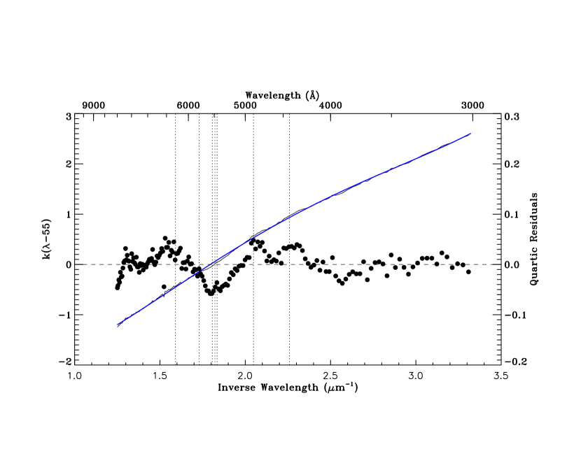
Figure 1: Mean of 71 MW curves determined by Paper VII and described in detail in §2, along with a quartic fit (blue curve) to the mean and $10\times$ the mean of the residuals. The residuals for individual curves in the sample can be nearly twice as large or almost nonexistent. The vertical dotted lines give the positions of the strong DIBs listed in Table 1 (given in § 3).

3 Empirical Measurements of the ISS

In this section, we fit the curves with a low order polynomial. We then examine the residuals of the polynomial fits, i.e., the ISS. We analyze the variability of the residuals in two ways. First, we quantify its strength and demonstrate that it is related to the amplitude of the 2175 Å bump (a result anticipated by Walker et al., 1980). Second, we analyze variations in the shape of the ISS and show that most of it can be captured by only three parameters.

To begin, we interpolate the curves over the locations of interstellar lines and those DIBs from the list given by Herbig (1995) that we could identify in our spectra. This allows our analysis to concentrate only on ISS features. The interstellar features removed are listed in Table 1. The curves were then smoothed by a Gaussian with a FWHM of 100 Å. Smoothing accomplishes two things: 1) it suppresses features with characteristic widths less than 100 Å (eliminating any residual influence of DIBs) and, 2) it reduces the “offset error” described below.

We can also use the smoothed and unsmoothed data to derive a measure of the mean error affecting the data. First, we subtract each 999 point spectrum with the ISM features removed from the version of itself convolved with the 100 Å FW Gaussian. This difference should capture most of the high frequency, random noise in the data. Next, the RMS of these differences at each wavelength for all of the observations is used to provide a representation of the wavelength dependence of the errors for the entire sample. Finally, the RMS of this wavelength array is used to derive a “representative”, mean error affecting the data. The value that results from this process is $\sigma_{obs}=0.0373$.

Table 1: Interstellar Features

Type	$\lambda$ (Å)	$\lambda^{-1}$ ($\mu^{-1}$)
Ca II	3933.66	2.54
Ca II	3968.47	2.52
Na I	5889.95	1.70
Na I	5895.92	1.70
K I	7664.91	1.30
K I	7698.97	1.30
DIB	4428.00	2.26
DIB	4882.00	2.05
DIB	5450.30	1.83
DIB	5487.50	1.82
DIB	5535.00	1.81
DIB	5780.45	1.73
DIB	6283.86	1.59

3.1 Magnitude of the ISS

We assume that the curves can be represented by a set of $N_{f}$ feature profiles, $\phi(\lambda-55)_{i}$, whose shapes are unspecified, and a background continuum that can be characterized by a polynomial of order $N_{p}$. In this case, an extinction curve can be expressed as

$$k(\lambda-55)=\sum_{i=1}^{N_{f}}a_{i}^{0}\phi(\lambda-55)_{i}+\sum_{j=0}^{N_{p}}b_{j}^{0}\lambda^{j}$$ (2)

Without model profiles for guidance, weak, broad structures, such as the ISS, are difficult to quantify. Unlike sharp features, such as DIBs, choosing continuum points is problematic. It is difficult to decide where the “continuum” begins and ends and whether a perceived continuum point is actually affected by the overlap of nearby features. In the end, any such procedure becomes highly subjective. Because of these difficulties, we begin our analysis with a different approach for measuring the ISS. Instead of attempting to fit the features with a set of profiles or to determine the underlying continuum, we examine the magnitudes of the residuals of the curves after they are fit by low order polynomials. Specifically, the residuals, $r(\lambda-55)$, are given by

$$r(\lambda-55)=k(\lambda-55)-\sum_{j=0}^{N_{p}}b_{j}\lambda^{j}$$ (3)

where the $b_{j}$ differ from the $b^{0}_{j}$ because they are fits to the entire curve, including the ISS. Consequently, they are affected by the ISS at some level. Experimentation showed that a fourth order polynomial (a quartic) adequately captures the overall shape of the curves and that higher order polynomials do not improve the fits.

After the smoothing and the removal of a quartic continuum, the features in the residuals have full widths between about 100 and 1200 Å, where the upper limit is the total wavelength interval divided by 4 (for the 4 zeros of a 4-th order polynomial). Features larger than 1200 Å are captured by the polynomial coefficients, while features less than 100 Å are lost, but should stand out in the raw spectra (the ISM lines and DIBs). As expected from Paper VII, the coefficients of the linear and quadratic terms are correlated with $R(V)\equiv A(V)/E(B-V)$, and we return to this correlation in § 4.2.

Figure 2 shows the individual residuals and their mean. The dotted curves are for stars with $E(44-55)<0.5$ mag, where the effect of mismatches between the observations and the best fitting model atmospheres used to create the curves are exaggerated (see Massa et al., 1983, for a discussion of mismatch errors). A few things are immediately apparent. First, the general structure is repeatable and present at some level in all of the well defined curves. Second, the broad depression in the extinction between $1.5\lesssim x\lesssim 2.0$ $\mu^{-1}$(where $x\equiv\lambda^{-1}$), which is normally associated with the VBS, is clearly present. Third, the VBS depression is actually a minimum surrounded by at least three distinct peaks, near $x=1.6$, 2.05, and 2.25 $\mu^{-1}$($\lambda=$4400, 4800 and 6600 Å). This is the same general structure first reported by Hayes et al. (1973). Finally, we note that the three distinct peaks in the ISS occur in the vicinity of the three strong DIBs at 4428, 4882 and 6384 Å (see Table 1).

The repeatability of the features validates the approach used in Paper VII to construct the curves, since the same features appear in curves derived from stars with very different physical parameters and a wide range in color excesses – indicating that these features are not a result of spectral mismatch between observed spectra and model flux calculations. The large scatter between $x=2.7$ and 2.9 $\mu^{-1}$ results from small mismatches between the models and the observations in the vicinity of the Balmer Jump, which are amplified in curves produced from stars with smaller $E(B-V)$ values. It appears that the models or our fitting procedures may need to be refined in this region.

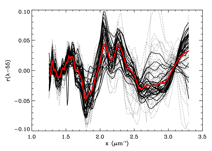
Figure 2: Individual $r(\lambda-55)$ curves (black) and their mean (red) plotted against inverse wavelength. Dotted and solid lines are used to denote curves derived from stars with $E(44-55)$ less than or greater than 0.5 mag, respectively.

We now require an objective means to measure the strength of the ISS. For lack of a better measure, we adopt the root mean square (RMS) of the residuals to measure its total strength. This is given by

$$RMS[r(\lambda-55)]\equiv\sqrt{\frac{1}{M_{\lambda}}\sum_{k=1}^{M_{\lambda}}r(\lambda_{k}-55)^{2}}$$ (4)

where $M_{\lambda}=999$. Note that $RMS[r(\lambda-55)]$ is also influenced by random, point to point measurement errors which create an additive term under the radical. This term creates an “offset error” (referred to above), in the sense that the measure can never be exactly zero, due to the random contribution. Further, in very noisy data the random errors can dominate the measurements. This was the motivation for aggressively smoothing the data with a 100 Å Gaussian, which should minimize the random contribution. Without the smoothing, there would be an additional term under the radical in equation (4) of order $\sigma_{obs}$. This term would introduce considerable scatter in Figure 3 and prohibit curves with no features whatsoever from approaching zero.

We next examine correlations between $RMS[r(\lambda-55)]$ and $R(V)$ and properties of the 2175 Å bump. Fitzpatrick & Massa (1986) parameterize the 2175 Å bump with a constant, $c$, times a Drude profile of the form

$$D(x,x_{i},\gamma_{i})=\frac{x^{2}}{(x^{2}-x_{i}^{2})^{2}+x^{2}\gamma_{i}^{2}}.$$ (5)

The maximum value, or amplitude, of the term is $a(2175)=c/\gamma^{2}$ and its area is $\pi c/(2\gamma)$ (see Fitzpatrick & Massa, 1986).

Figure 3 shows the relations between $RMS[r(\lambda-55)]$ and $R(V)$ (top) and $a(2175)$ (bottom). Values of $a(2175)$, and $R(V)$ are from Paper VII. It is clear that $RMS[r(\lambda-55)]$ is poorly correlated with $R(V)$. In contrast, our measure of the ISS structure is strongly correlated with $a(2175)$. Considering the crudeness of our current measure, this seems rather remarkable.

Figure 3: $RMS[r(\lambda-55)]$ plotted against $R(V)$ (top) and bump amplitude, $a(2175)$ (bottom). Large, filled symbols are for values derived from curves with $E(44-55)\geq 0.5$ mag, which should be most accurate.

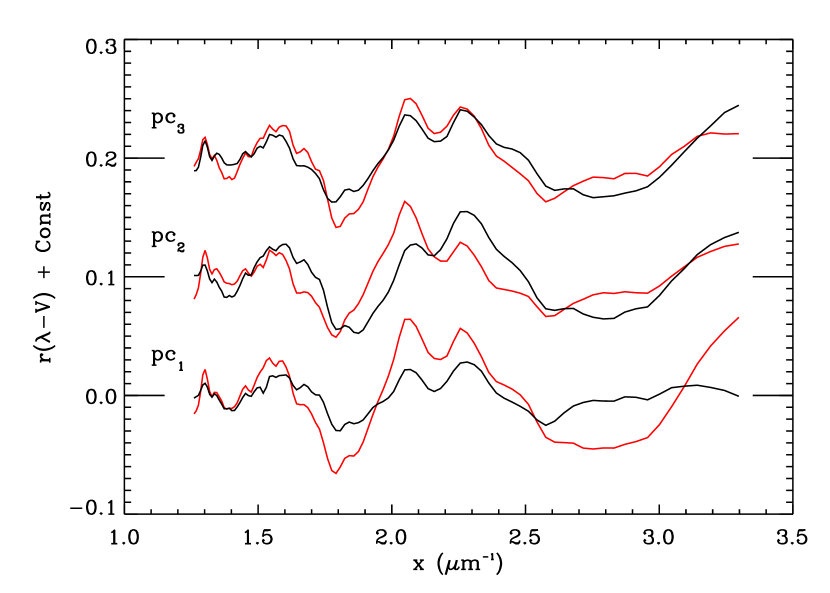
Figure 4: The effects of the three largest principal components of $r(\lambda-55)$ on the sample mean plotted against inverse wavelength. Each pair of curves shows the effect of adding (black) and subtracting (red) the PC to the mean. The zero point of each set of curves is shown by the large tick marks and the curves are arranged with the largest PC at the bottom. The variations caused by the PCs are scaled by the magnitude of their variances.

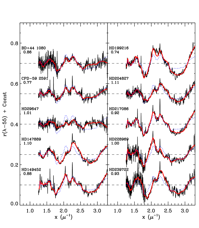
Figure 5: Plots of the $r(\lambda-55)$ at 5 Å sampling for the 10 most reddened stars in our sample as functions of inverse wavelength. The name of the star and its $E(B-V)$ are given for each curve. The red curves are approximations using the sample mean and the first three PCs. The sample mean (dotted blue) is over plotted on each curve for comparison and the dashed lines indicate the zero point for each curve. The sharp peaks are due to the interstellar features listed in Table 1.

3.2 Wavelength dependence of the ISS variations

We next examine the systematic variations in the ISS using principal component decomposition (see Massa, 1980, for a discussion of the use of component analysis to characterize extinction). In this analysis, the data were binned even further, to 50 Å, which is the minimum possible sampling for the data, which are smoothed by a 100 Å Gaussian. The result is a set of 99 point spectra. These were used to construct a covariance matrix of excesses. We use excesses, $E(44-55)r(\lambda-55)$, because they give larger weight to the more well defined curves, derived from stars with larger reddenings. The covariance matrix is given by

$$S_{ij} = \frac{1}{N-1}\sum_{n=1}^{N}[r(\lambda_{i}-55)^{(n)}-\langle r(\lambda_{i}-55)\rangle]E(44-55)^{(n)}$$ (6)

$$\times[r(\lambda_{j}-55)^{(n)}-\langle r(\lambda_{j}-55)\rangle]E(44-55)^{(n)}$$

where $N=71$, the number of stars in the sample, $i$ and $j$ vary from 1 to $N_{\lambda}=99$, the number of wavelength points, and

$$\langle r(\lambda_{i}-55)\rangle=\sum_{n=1}^{N}r(\lambda_{i}-55)^{(n)}E(44-55)^{(n)}/\sum_{n=1}^{N}E(44-55)^{(n)}$$ (7)

is the weighted mean. The $N_{\lambda}$ eigenvalues, $e_{i}$, and eigenvectors (or principal components, PCs), $v(\lambda)_{i}$, of this matrix give the magnitudes and shapes of the variations, in order of the magnitudes of the variances. We note that the matrix $S_{ij}$ is singular, since there are more wavelength points than objects in the sample. However, this simply means that the $N_{\lambda}-N=32$ smallest eigenvalues are zero.

A given residual, $r(\lambda-55)^{(n)}$, can be approximated in terms of a specified number, $N_{pc}$, of PCs as

$$r(\lambda-55)^{(n)}\approx\sum_{i=1}^{N_{pc}}\alpha_{i}^{(n)}v(\lambda)_{i}$$ (8)

where the relation is exact when $N_{pc}=N_{\lambda}$, and the coefficients are given by

$$\alpha_{i}^{(n)}=\sum_{k=1}^{N_{\lambda}}v(\lambda_{k})_{i}r(\lambda_{k}-55)^{(n)}$$ (9)

For any criterion of the significance of the principal components, some estimate of the observational errors is required. For this purpose, we adopt $\sigma_{obs}/\sqrt{10}=0.0118$, where the numerical radical accounts for the rebinning to 99 points. This value can be compared to the magnitudes of the eigenvalues derived from the sample covariance matrix. The ratio of the square roots of the 5 largest eigenvalues to this value are: 4.92, 3.93, 2.26, 1.57 and 1.34. Consequently, we see that the variance along the first 3 components are larger than twice the expected mean error, and these are considered significant. Furthermore, if we define the fraction of the total variance due to a particular component, $e_{i}$, as $e_{i}/\sum_{1}^{N_{\lambda}}e_{n}$, the first three components account for 44, 31 and 10% of the total variance, respectively, for a total of 85%. In contrast, the fourth component accounts for less than 4%, a value more representative of the expected random errors. Figure 4 shows how the three largest PCs affect the mean residual. The effect of each PC has been scaled by the magnitude of its associated eigenvalue. The first PC appears to describe the relative strength of the two peaks near 2.1 $\mu^{-1}$ relative to the minima near 1.8 and 2.8 $\mu^{-1}$. The major effects of the second PC are changing the relative strengths of the two peaks near 2.1 $\mu^{-1}$ and making the minimum near 2.8 $\mu^{-1}$ weaken in concert with the short wavelength 2.1 $\mu^{-1}$ peak. The dominant effect of the third component is to change the relative strengths of the two minima, weakening the one near 1.8 $\mu^{-1}$ while strengthening the one near 2.8 $\mu^{-1}$. It is difficult to interpret the variability at the shortest wavelengths. It could be due to the wing of another feature with a peak at $\lambda<3000$ Å, or an artifact of the continuum fitting.

Figure 5 shows the residuals of the 10 most reddened stars in our sample. For each star, the plots show: the unsmoothed residuals, the representation of the residuals given by the mean and the three largest PCs and, the sample mean residual for comparison. Note that the first three PCs produce excellent fits to all of the curves, except for the interstellar lines and DIBS listed in Table 1. This suggests that there may be no more than three parameters influencing the ISS. As expected from Figure 2, the features can vary significantly in strength (compare HD 29647 and HD 199216), and the strengths of all three peaks vary relative to one another (compare HD 147889 and HD 228969). The feature widths also vary, with the feature near 1.6 $\mu^{-1}$ (which could have more than one component) showing the largest variation (compare BD$+44^{\circ}1080$ and CPD$-59^{\circ}2591$). The position of the broad minimum near 1.8 $\mu^{-1}$, which is normally attributed to the VBS, appears to shift depending on the relative strengths of the three peaks. This leads us to believe that its position is influenced by the wings of the surrounding absorption peaks.

4 Modeling the ISS

In this section, we describe an ad hoc model which enables us to isolate and quantify the major features seen in the residuals. Unlike the previous section, we use the resampled, but unsmoothed curves. Inspection of the mean residual curve shown in Figure 2 and the individual residuals shown in Figure 5 suggests that the most prominent aspects of the curves can be represented by a smooth background extinction and 3 distinct features centered near the strong DIBs at 4428, 4882, and 6383 Å. The upswings in the residuals at each end of the wavelength interval are most likely artifacts of the polynomial background fit. We also search for correlations among the parameters used to fit the data, and discuss how such correlations might arise.

4.1 Fitting the curves

Each of the three strongest features are modeled as a Drude profile of the form given by equation (5). Drude functions are appealing because they have a solid physical basis and have been shown to provide excellent representations of dust extinction (Fitzpatrick & Massa, 1986) and emission (e.g. Draine & Li, 2001). As previously stated, a quartic adequately describes the overall shapes of the curves. Consequently, we fit each curve with the following function

$$k(\lambda-V)=\sum_{i=1}^{3}c_{i}D(x,x_{i},\gamma_{i})+\sum_{j=0}^{4}d_{j}x^{j}$$ (10)

Altogether, this model contains 9 free parameters to describe the features: three $c_{i}$, $x_{i}$, and $\gamma_{i}$. These, along with the five $d_{j}$, were determined by non-linear least squares, using the Interactive Data Language (IDL) procedure MPFIT developed by Markwardt (2009). We also use the notation $a(\lambda_{i})=c_{i}/\gamma_{i}^{2}$, where $\lambda_{i}=x_{i}^{-1}$, to denote the amplitude (maxima) of the profiles. Because all of the stars have been fit in the UV as well ( Paper VII, ), parameters for the 2175 Å Drude profile are available for each. Consequently, we were able to remove the contribution to the curves of the long wavelength tail of the 2175 Å Drude profile (although this had little influence on the results). The regions of interstellar lines and the strong DIBs listed in Table 1 were given zero weight. In contrast, the regions near the Drude peaks were given 9 times the weight of the surrounding regions. This restrains the fitting routine from using the tails of the Drude profiles to help the overall agreement of purely continuum regions and emphasizes the influence of the positions and widths of the profiles . We also constrained the $\gamma_{i}$ to be $\leq 0.5$ $\mu^{-1}$. This constraint keeps the Drude profiles from getting so wide that they become entangled in the continuum fitting.

We note that equation (10) is, in fact, an approximation. The observed curves actually have the form

$$k(\lambda-55) = \frac{E(\lambda-55)_{D}+E(\lambda-55)_{B}}{E(44-55)_{D}+E(44-55)_{B}}$$ (12)

$$\simeq \left[\frac{E(\lambda-55)_{D}}{E(44-55)_{B}}+k(\lambda-55)_{B}\right]$$

$$\times\left[1-\frac{E(44-55)_{D}}{E(44-55)_{B}}\right]$$

where the subscripts $D$ and $B$ refer to the Drude and background contributions, and equation (12) follows since $E(44-55)_{D}<<E(44-55)_{B}$. The term inside the first set of brackets in equation (12) can be rewritten as

$$\frac{E(\lambda-55)_{D}}{E(44-55)_{B}}+k(\lambda-55)_{B} = \sum_{i}\frac{c^{0}_{i}}{E(44-55)_{B}}D(\lambda-55)_{i}$$ (13)

$$+k(\lambda-55)_{B}$$

which has the same form as equation (10). We see that the second term in this equation cannot affect the Drudes and that the $c_{i}$ determined from the fits to equation (10) are actually proportional to $c^{0}_{i}/E(44-55)_{B}$. The second bracketed term in equation (12) is a multiplicative constant for each line of sight which is $\lesssim 1$. Consequently, it can rescale everything but it cannot affect the $x_{0i}$, $\gamma_{i}$, or the ratios of the $c_{i}$. Consequently, equation (10) is a good approximation, but we need to keep in mind that the $c_{i}$ derived from the fits are actually $\simeq c_{i}^{0}/E(44-55)_{B}$, where the $c^{0}_{i}$ can be directly related to physical parameters described in § 4.2.

Table 3 lists some properties of the fit parameters for the 24 stars in our sample with $E(44-55)\geq 0.5$ (values for the entire sample are very similar). For each parameter listed in the first column, the Table gives: mean, standard deviation, minimum, maximum, and range, defined as $100\times$(max–min)/mean. It is immediately apparent that the $x_{i}$ values are quite robust and that their total ranges vary by only a few percent. Consequently, we refer to them as the 4370, 4870 and 6800 Å features hereafter. In contrast, all of the other parameters have ranges that vary by more than a factor of 2.

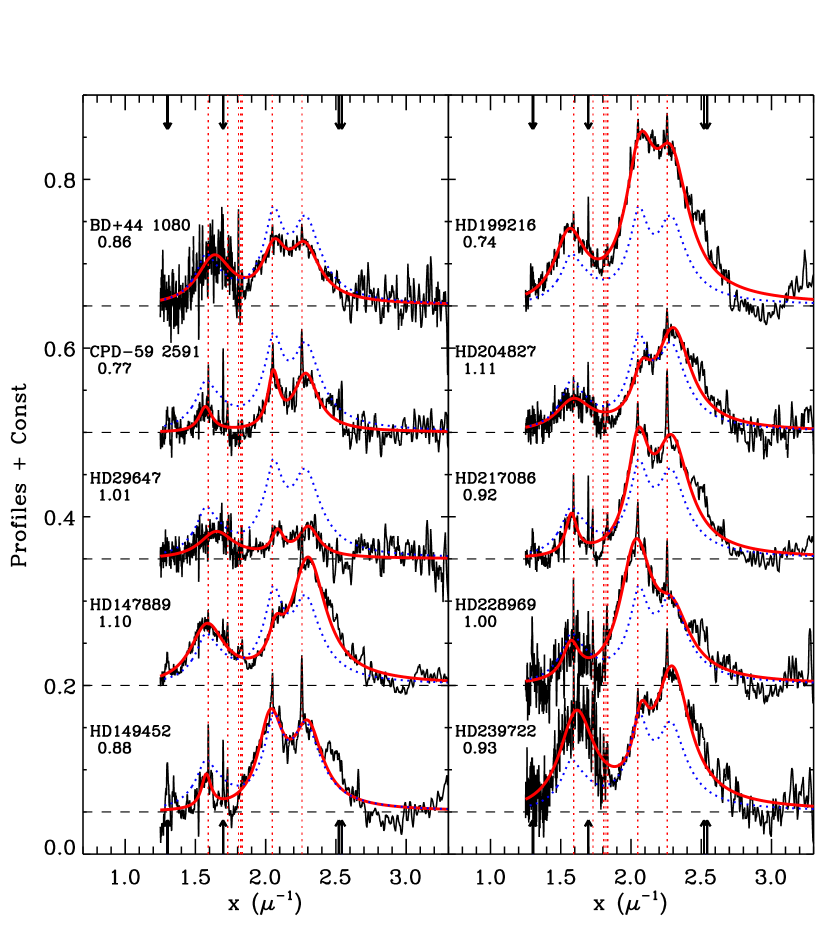
Figure 6: Plots of the profile fits for the 10 most reddened stars in our sample as functions of inverse wavelength. The name of the star and its $E(B-V)$ are given for each curve. The thick red curves are the Drude fits, the dotted blue curve is the sample mean fit, the black curve is the data and the dashed lines give the zero point for each profile. The arrows show the positions of interstellar absorption lines (which appear as excess extinction) and the vertical dotted red lines show the positions of the strong DIBs listed in Table 1.

Table 2: Fit Parameters

Star	$a_{l}\times 10^{3}$	$a_{2}\times 10^{3}$	$a_{3}\times 10^{3}$	$\gamma_{1}$	$\gamma_{2}$	$\gamma_{3}$	$x_{10}$	$x_{20}$	$x_{03}$	$b_{0}$	$b_{1}$	$b_{2}$	$b_{3}$	$b_{4}$
BD+44 1080	4.608	3.005	4.009	0.300	0.230	0.262	1.636	2.065	2.285	9.408	-27.801	14.10	18.91	-17.21
BD+56 517	2.140	6.139	6.854	0.176	0.209	0.251	1.569	2.057	2.290	5.270	-4.389	-34.87	63.59	-32.06
BD+56 518	8.050	7.058	8.537	0.300	0.231	0.300	1.577	2.052	2.301	6.000	-7.353	-31.61	63.44	-32.85
BD+56 576	1.664	6.462	3.377	0.151	0.205	0.195	1.564	2.057	2.285	5.071	-2.996	-37.72	65.43	-32.17
BD+69 1231	0.423	3.985	1.087	0.083	0.182	0.109	1.573	2.068	2.281	12.913	-54.559	86.42	-63.74	16.75
BD+71 92	11.018	10.219	1.806	0.300	0.256	0.158	1.609	2.068	2.273	6.851	-8.928	-40.25	87.38	-48.11
CPD-41 7715	0.228	2.048	1.225	0.086	0.171	0.148	1.571	2.052	2.290	3.684	4.846	-51.30	72.90	-32.61
CPD-57 3507	7.548	0.543	0.304	0.275	0.088	0.056	1.585	2.058	2.305	2.203	15.575	-78.23	100.73	-42.57
CPD-57 3523	0.937	1.057	10.445	0.148	0.108	0.300	1.668	2.069	2.307	4.789	-2.619	-35.72	61.84	-30.92
CPD-59 2591	0.439	0.791	3.192	0.121	0.114	0.218	1.569	2.056	2.289	1.918	15.054	-72.46	92.24	-39.88
CPD-59 2600	0.277	1.113	4.024	0.085	0.118	0.216	1.579	2.053	2.307	3.477	4.449	-46.34	64.44	-28.96
CPD-59 2625	7.622	4.809	0.015	0.300	0.232	0.010	1.621	2.040	2.236	3.714	8.139	-67.51	98.29	-45.67
HD13338	2.480	9.761	8.707	0.174	0.230	0.271	1.561	2.059	2.284	5.317	-5.032	-33.28	62.44	-32.01
HD14250	1.869	13.452	8.031	0.162	0.268	0.278	1.561	2.049	2.296	5.512	-5.677	-33.09	63.22	-32.53
HD14321	1.147	4.361	4.823	0.139	0.187	0.232	1.565	2.056	2.288	6.718	-14.099	-9.58	34.12	-19.36
HD17443	0.003	0.218	2.180	0.006	0.073	0.192	1.664	2.084	2.265	15.595	-70.847	124.15	-103.36	32.81
HD18352	1.682	5.501	13.092	0.154	0.194	0.300	1.563	2.054	2.285	7.070	-17.966	1.55	21.90	-14.74
HD27778	6.604	1.408	3.910	0.300	0.152	0.224	1.622	2.072	2.269	6.868	-11.659	-25.22	61.91	-34.78
HD28475	6.932	4.309	1.314	0.300	0.178	0.127	1.570	2.061	2.286	3.113	9.944	-69.94	100.94	-46.48
HD29647	2.711	0.249	0.656	0.300	0.100	0.142	1.628	2.093	2.314	8.650	-26.976	24.81	-7.42	-1.38
HD30122	10.780	3.551	12.304	0.300	0.169	0.300	1.578	2.072	2.289	2.382	14.026	-80.90	115.66	-53.95
HD30675	9.493	0.307	11.180	0.300	0.092	0.288	1.625	2.079	2.302	3.324	8.898	-69.30	102.72	-48.55
HD37061	0.080	0.060	0.048	0.056	0.035	0.051	1.545	2.050	2.306	2.082	14.118	-66.36	78.32	-30.74
HD38087	0.468	13.017	0.331	0.101	0.300	0.085	1.565	2.005	2.281	1.108	24.079	-103.18	133.32	-59.14
HD40893	6.185	3.415	14.550	0.255	0.160	0.300	1.593	2.053	2.294	4.220	2.928	-56.07	91.87	-45.83
HD46106	1.137	5.244	5.596	0.132	0.200	0.229	1.566	2.051	2.291	5.836	-9.891	-15.82	36.12	-18.25
HD46660	3.057	2.170	8.377	0.237	0.146	0.275	1.585	2.054	2.304	5.574	-7.491	-24.70	50.10	-25.77
HD54439	5.813	1.690	10.967	0.288	0.119	0.300	1.594	2.062	2.308	6.653	-14.204	-8.62	32.39	-17.83
HD62542	5.204	0.590	2.163	0.300	0.116	0.253	1.679	2.057	2.280	7.013	-10.168	-32.61	72.73	-40.38
HD68633	0.569	4.630	0.607	0.118	0.280	0.115	1.555	2.014	2.301	2.569	13.145	-72.42	95.08	-41.13
HD70614	1.230	8.159	1.201	0.137	0.237	0.150	1.562	2.034	2.287	1.234	22.737	-100.07	130.06	-56.67
HD91983	2.926	0.521	10.432	0.247	0.076	0.300	1.642	2.080	2.281	8.464	-29.332	34.71	-18.44	2.71
HD92044	3.435	2.221	11.762	0.251	0.163	0.300	1.597	2.069	2.292	6.795	-19.126	13.28	-1.02	-1.94
HD93028	0.344	1.130	1.966	0.087	0.108	0.146	1.562	2.055	2.283	5.167	-5.312	-27.06	50.09	-26.23
HD93222	0.002	0.842	4.427	0.004	0.108	0.222	1.593	2.061	2.308	5.783	-15.826	14.78	-11.54	4.41
HD104705	0.113	0.776	8.002	0.049	0.104	0.281	1.594	2.062	2.289	6.839	-18.225	7.30	11.19	-9.15
HD110336	4.604	0.476	2.660	0.264	0.111	0.182	1.580	2.092	2.294	6.591	-15.057	-2.17	20.12	-11.60
HD110946	8.130	4.056	6.718	0.300	0.188	0.300	1.567	2.057	2.267	4.475	1.333	-48.36	76.06	-35.86
HD112607	0.255	1.595	1.861	0.081	0.158	0.146	1.566	2.072	2.278	7.202	-18.444	3.87	17.13	-12.11
HD142096	0.488	0.189	0.015	0.085	0.045	0.010	1.550	2.055	2.295	4.061	3.028	-47.11	67.80	-30.44
HD142165	0.034	0.386	0.243	0.023	0.060	0.054	1.550	2.055	2.288	15.724	-78.050	159.93	-162.83	64.44
HD146285	0.146	7.655	0.214	0.070	0.283	0.067	1.561	2.033	2.285	7.644	-20.264	7.74	11.79	-9.42
HD147196	1.997	0.004	4.262	0.158	0.007	0.300	1.655	2.073	2.171	10.089	-39.121	61.55	-56.01	22.40
HD147889	6.211	0.592	13.005	0.300	0.129	0.300	1.583	2.076	2.305	1.700	13.447	-63.59	78.67	-33.07
HD149452	0.332	6.188	7.209	0.093	0.239	0.277	1.575	2.034	2.308	3.698	5.096	-54.50	80.27	-37.41
HD164073	1.019	6.958	0.012	0.114	0.295	0.011	1.592	1.950	2.325	4.140	4.783	-55.60	80.46	-37.24
HD172140	3.504	0.706	8.434	0.226	0.087	0.231	1.577	2.058	2.303	4.687	-6.024	-16.05	26.81	-10.86
HD193322	0.378	6.065	1.764	0.099	0.230	0.154	1.563	2.038	2.294	5.682	-3.931	-42.85	78.98	-41.00
HD197512	3.506	7.942	6.571	0.207	0.224	0.253	1.562	2.064	2.276	5.575	-6.276	-31.69	62.14	-32.22
HD197702	0.910	7.500	16.113	0.112	0.222	0.300	1.601	2.074	2.285	9.736	-36.463	47.57	-26.77	3.71
HD198781	0.192	1.661	8.966	0.077	0.140	0.300	1.553	2.050	2.274	6.670	-17.209	5.45	10.85	-7.69
HD199216	6.576	11.963	12.661	0.278	0.272	0.300	1.562	2.069	2.295	7.772	-22.748	12.66	10.66	-10.44
HD204827	3.547	1.745	10.317	0.300	0.183	0.300	1.591	2.079	2.307	10.212	-37.766	48.84	-28.49	5.28
HD210072	7.334	2.680	4.819	0.300	0.169	0.251	1.616	2.048	2.269	10.181	-33.035	27.94	1.98	-9.11
HD210121	0.088	0.452	1.629	0.059	0.108	0.164	1.546	2.079	2.286	14.630	-64.916	112.03	-94.18	30.96
HD217086	0.605	5.127	11.475	0.113	0.204	0.300	1.573	2.052	2.297	5.083	-4.333	-32.83	59.93	-30.56
HD220057	5.044	1.226	1.557	0.241	0.121	0.141	1.566	2.064	2.293	6.119	-9.277	-21.49	45.39	-22.93
HD228969	1.390	15.484	5.905	0.162	0.300	0.300	1.577	2.033	2.304	4.088	8.469	-78.76	123.01	-59.90
HD236960	10.749	5.502	13.059	0.300	0.206	0.300	1.591	2.058	2.293	4.703	-1.371	-41.20	69.07	-33.43
HD239693	10.237	3.043	10.555	0.300	0.174	0.299	1.569	2.064	2.294	3.735	5.604	-59.06	88.99	-41.62
HD239722	9.571	1.526	14.170	0.300	0.147	0.300	1.619	2.077	2.298	5.025	-1.484	-46.51	81.58	-41.37
HD239745	1.359	7.758	10.689	0.153	0.245	0.300	1.561	2.057	2.294	5.649	-8.412	-22.11	47.34	-24.92
HD282485	3.507	2.253	9.103	0.222	0.166	0.249	1.616	2.085	2.303	6.738	-15.299	-7.34	34.74	-21.25
HD292167	0.387	2.690	14.033	0.081	0.158	0.300	1.588	2.053	2.297	5.649	-10.217	-13.57	34.76	-19.09
HD294264	3.908	7.970	0.006	0.300	0.300	0.012	1.605	1.989	2.290	-2.057	43.472	-144.91	171.47	-72.25
HD303068	10.141	7.196	5.626	0.300	0.260	0.248	1.651	2.061	2.323	2.078	21.228	-107.95	152.48	-71.17
NGC 2244 11	1.543	2.904	10.803	0.148	0.151	0.280	1.565	2.056	2.298	5.715	-10.921	-9.84	27.09	-13.89
NGC 2244 23	8.349	2.255	5.931	0.300	0.156	0.247	1.594	2.058	2.292	2.755	13.427	-80.73	114.42	-52.42
Trumpler 14	0.666	0.530	7.158	0.122	0.097	0.300	1.604	2.065	2.289	3.506	3.749	-43.21	59.35	-25.85
Trumpler 14	1.215	1.883	5.946	0.181	0.167	0.300	1.599	2.068	2.309	4.253	0.117	-37.12	55.30	-25.09
VSS VIII-10	7.541	6.278	3.586	0.300	0.300	0.300	1.678	1.960	2.194	6.582	-6.723	-40.22	77.67	-40.98

Figure 6 shows the profile portion of the fits, i.e., the fit minus the quartic contribution, for the 10 most reddened stars in our sample. The overall quality of the fits is good, but it is also apparent that some aspects of the curves are not fit particularly well by our simple model (e.g., the blue edge of the curves and the blue wing of the 4370 Å profile). While all the features are, in general, rather weak, their strengths vary significantly, from $\lesssim 0.05$ in HD 29647, to $\gtrsim 0.20$ in HD 199216 and HD 239722, where the first has a very weak 2175 Å bump and the latter two quite strong ones (see Paper VII, ).

Plots of correlations among the individual fit parameters show that the amplitudes of the features, $a(4370)$ and $a(4870)$, correlate well with $a(2175)$, but that $a(6300)$ does not. Figure 7 shows the correlation between $a(4370)+a(4870)$ and $a(2175)$. Although there is a clear correlation between these two quantities, the relation is not quite as strong as the one between the RMS of the residuals and $a(2175)$ shown in Figure 3. This is, no doubt, because our simple model does not capture all of the more complex structure that is related to $a(2175)$ and because the derived parameters may be influenced by the continuum fit.

4.2 Relations among the fit parameters

Since 3 PCs can explain 85% of the variability, there should be several constraints among the 9 fit parameters used to fit the three profiles. Three constraints can be found by fixing the central positions of the three $x_{0i}$, since their variance is so small. When this is done, the quality of the fits is hardly affected. We searched for additional relations among the other parameters and noticed that the scale factors, $c_{i}$ and the widths, $\gamma_{i}$ are related. Figure 8 shows the $c_{i}-\gamma_{i}$ relations for all three features. A different constant for each feature has been added to the $\log\gamma$, vertically shifting the points, so that each feature can be seen to follow a simple linear relation, which has a slope 3. Notice that several of the points for the 6630 Å feature and a few for the 4370 Å one, form horizontal lines near $\log\gamma\simeq-0.6$. This is due to the constraint enforced on $\gamma_{i}$ in the fitting routine described above. Nevertheless, over most of the range, the vast majority of the points fall along a line, which implies that there are constants, $A_{i}$, such that

$$c_{i}=\frac{c_{i}^{0}}{E(44-55)_{B}}=A_{i}\gamma_{i}^{3}\;\;,$$ (14)

where $A_{i}=0.35,0.70,$ and 0.45, for the 6300, 4870, and 4370 Å features, respectively. These relations can be used to eliminate the $c_{i}$, leaving the $\gamma_{i}$ as the only free parameters in the fits. When this was done, the fits degraded significantly. However, when the constraints were only applied to the 4870 and 4370 Å features, and both $c$ and $\gamma$ were allowed to be free for 6300 Å, the quality of the fits became comparable to that obtained when no constraints are applied. As a result, we can find 5 constraints, implying that only 4 free parameters are needed to fit all three optical features.

The question that naturally arises is whether the parameters of the 2175 Å bump follow the same relation. Figure 9 extends the range shown in Figure 8, to include the 2175 Å bump. In this case, $A=4.0$. Although there is considerable scatter, it appears that the lower envelope of the 2175 Å parameters also follows a line of slope 3.

We now consider what the $c\propto\gamma^{3}$ relations might imply. To begin, we adopt a very simplistic model which consists of one grain size of Drude absorbers and one grain size of background absorbers along each line of sight. For a single population of Drude particles, $N_{D}\propto c^{0}/\gamma$, where $N_{D}$ is the number of absorbers (see Bohren & Huffman, 1983). We also assume that $N_{B}\propto E(B-V)_{B}$, where $N_{B}$ is the number of background absorbers. As a result, equation(14) becomes $N_{D}/N_{B}\propto\gamma^{2}$. In the Drude model, $\gamma\propto 1/r_{D}$, where $r_{D}$ is the radius of the absorbers and their geometric cross section is $a_{D}\propto r_{D}^{2}$. This gives $N_{D}/N_{B}\propto a_{D}^{-1}$. If we also assume that $N_{B}$ is fixed, then the previous relation implies that when the Drude grains are small, there are relatively more of them along the line of sight compared to background absorbers and when they are large, there are relatively fewer. In addition, the total mass in Drude grains, $M_{D}$, is related to $r_{D}$ by $M_{D}\propto\rho N_{D}r_{D}^{3}$. Utilizing the previous result, that $N_{D}\propto r_{D}^{-2}$ implies that $M_{D}\propto r_{D}$, i.e., there is less mass in the Drude grains when they are smaller. Thus, the empirical relations given by eq. (14) imply that the relative number of Drude absorbing grains may be similar along all Milky Way lines of sight, but that less total mass resides in the Drude grains when they are smaller. We emphasize that this model is extremely simplistic and only meant to illustrate how the constraints could influence a more comprehensive grain model.

Figure 7: Combined amplitudes of the 4370 and 4870 Å features plotted against the amplitude of the 2175 Å UV bump. Large, filled symbols are for values derived from curves with $E(44-55)\geq 0.5$ mag, which should be most accurate.

Figure 8: Log-log plot of the $\gamma$s versus the scale factors for all of the features. Symbols are: crosses for 4370 Å, filled circles for 4870 Å and open circles for 6300 Å. The line has a slope of 3, which represents a cubic. To align the data, a single constant was added to all of the $\log\gamma$ data for each wavelength. Note that a few of the $\gamma$s for the 6300 and 4870 Å fits ran into the upper limit in the non-linear least squares routine, causing a horizontal row of points near $\log\gamma=-0.65$.

Figure 9: Log-log plot of the $\gamma$s versus the scale factors for all of the features including the UV 2175 Å bump. Symbols for the optical features are the same as in Figure 8 and the triangles represent the 2175 Å data. As in Figure 8, the line has a slope of 3 and the a single constant was added to all of the $\log\gamma$ data for each feature.

We also performed principal component analysis on the continuum polynomials derived for each curve. The two largest PCs account for nearly 90% of the continuum variation, 51 and 37%, respectively. The upper plot in Figure 10 shows the wavelength dependence of the two largest PCs, as well as a scaled version of the mean polynomial fit. The lower plot shows the relationship between the coefficients of the largest PC and $R(V)$. The excellent correlation should not be surprising, since it is well known that curves which “roll over” in the optical, i.e., are strongly influenced by the shape of the largest PC, are typically associated with large $R(V)$ values. We note that the maximum of the largest PC lies very near the maximum in the $dk(\lambda-55)/dR(55)$ curve given by Paper VII. However, it is shortward of the maximum in the second PC derived by Schlafly et al. (2016). This difference is most likely the result of the very different wavelength baselines used.

Figure 10: Top: The largest (solid) and second largest (dashed) principal components of the continuum fits, compared to a scaled version of the mean curve (dotted). Bottom: The components of the largest PC plotted against $R(V)$. Large, filled symbols are for values derived from curves with $E(44-55)\geq 0.5$ mag.

Table 3: Parameter properties

Name	Mean	$\sigma$	Min	Max	Range
	(mag)	(mag)	(mag)	(mag)	(%)
$a(4370)$	0.102	0.043	0.018	0.188	166
$a(4870)$	0.107	0.046	0.030	0.194	153
$a(6300)$	0.077	0.037	0.023	0.170	190
	( $\mu^{-1}$)	( $\mu^{-1}$)	( $\mu^{-1}$)	( $\mu^{-1}$)	(%)
$x_{1}$	2.288	0.012	2.26	2.31	2.2
$x_{2}$	2.054	0.013	2.08	2.01	3.6
$x_{3}$	1.587	0.027	1.66	1.55	6.7
$\gamma_{1}$	0.243	0.011	0.019	0.400	156
$\gamma_{2}$	0.179	0.007	0.030	0.288	144
$\gamma_{3}$	0.243	0.148	0.080	0.400	132

5 Summary

We have verified the reality of ISS features in extinction curves by demonstrating two properties. First, its strength is independent of the physical parameters of the star used to create a curve. This can be seen by comparing the features for HD 147889 (B2 V), and HD 149452 (O8 V) in Figures 5 and 6. Second, the strength of the ISS correlates with an interstellar feature, the strength of the 2175 Å bump. Further, as with the 2175 Å feature, curves of stars in the same region tend to have the same ISS strength. We then proceeded to determine the magnitude, wavelength dependence and variability of the ISS in two different ways.

In the first approach, we examined the residuals of the extinction curves relative to a smooth background that is modeled by a quartic. It was shown that the residual curves have three strong peaks whose relative strengths and widths vary substantially from one sight line to another, but whose central positions are relatively stable and located near the strong DIBs at 4428, 4882 and 6284 Å, suggesting a possible relation. It was also apparent that the VBS is actually a local minimum between absorption features. Next, we demonstrated that the magnitudes of the root mean square of the residuals – which give a crude measure of the strength of the ISS – are poorly correlated with $R(V)$, but strongly correlated with the strength of the 2175 Å bump. Finally, principal component analysis was used to reveal that most of the ISS variations can be captured by the first three PCs of the residuals, suggesting that as few as three physical parameters might be able to explain the variations.

In the second approach, we modeled the ISS with three Drude profiles in order to quantify its major structures. This simple model provides a reasonable fit to the ISS, although it has some small inadequacies. The fits showed that the feature locations are very stable, near $\lambda=4370$, 4870 and 6300 Å  and that the features contribute anywhere from a few percent to 20% of the extinction in those regions. Further analysis

showed that the strengths of the 4370 and 4870 Å features correlate with the strength of the 2175 Å UV bump, but the 6300 Å feature does not, and that none of the features correlate with $R(V)$. We found relations among the model parameters which can reduce them from 9 to 4, without a major loss of accuracy. Interpretation of these relations in terms of a simple dust model suggests that the density of dust producing the ISS is similar along all lines of sight, but distributed in different grain sizes. In addition, we verified that the strongest variation in the continuum extinction is the curvature, and that its strength is related to $R(V)$.

While it is hoped that our results will be useful for developing physical models of dust grains, they also have practical importance. Although the ISS is small, it should be taken into consideration if one wishes to achieve accurate fits to the SEDs of reddened stars. Also, the relation between the ISS features and the strength of the 2175 Å bump could be useful for estimating the strength of the 2175 Å bump in objects whose optical SEDs are either intrinsically smooth or well modeled but whose UV SEDs are poorly determined.

References

- Bohren & Huffman (1983) Bohren, C. F., & Huffman, D. R. 1983, New York: Wiley
- Clayton et al. (2003) Clayton, G. C., Gordon, K. D., Salama, F., et al. 2003, ApJ, 592, 947
- Draine & Li (2001) Draine, B. T., & Li, A. 2001, ApJ, 551, 807
- Fitzpatrick & Massa (1986) Fitzpatrick, E. L., & Massa, D. 1986, ApJ, 307, 286
- Fitzpatrick & Massa (2007) Fitzpatrick, E. L., & Massa, D. 2007, ApJ, 663, 320
- Fitzpatrick et al. (2019) Fitzpatrick, E. L., Massa, D., Gordon, K. D., et al. 2019, ApJ, 886, 108
- Gordon et al. (2009) Gordon, K. D., Cartledge, S., & Clayton, G. C. 2009, ApJ, 705, 1320
- Hayes et al. (1973) Hayes, D. S., Mavko, G. E., Radick, R. R., et al. 1973, Interstellar Dust and Related Topics, 83
- Herbig (1995) Herbig, G. H. 1995, ARA&A, 33, 19
- Lanz & Hubeny (2003) Lanz, T., & Hubeny, I. 2003, ApJS, 146, 417
- Markwardt (2009) Markwardt, C. B. 2009, Astronomical Data Analysis Software and Systems XVIII, 251
- Massa (1980) Massa, D. 1980, AJ, 85, 1651
- Massa et al. (1983) Massa, D., Savage, B. D., & Fitzpatrick, E. L. 1983, ApJ, 266, 662
- Schlafly et al. (2016) Schlafly, E. F., Meisner, A. M., Stutz, A. M., et al. 2016, ApJ, 821, 78
- Schild (1977) Schild, R. E. 1977, AJ, 82, 337
- Walker et al. (1980) Walker, G. A. H., Yang, S., Fahlman, G. C., et al. 1980, PASP, 92, 411
- Whiteoak (1966) Whiteoak, J. B. 1966, ApJ, 144, 305
- Whittet et al. (1976) Whittet, D. C. B., van Breda, I. G., & Glass, I. S. 1976, MNRAS, 177, 625
- York (1971) York, D. G. 1971, ApJ, 166, 65