Uniform error bounds of time-splitting spectral methods for the long-time dynamics of the nonlinear Klein–Gordon equation with weak nonlinearity

Abstract.

We establish uniform error bounds of time-splitting Fourier pseudospectral (TSFP) methods for the nonlinear Klein–Gordon equation (NKGE) with weak power-type nonlinearity and $O(1)$ initial data, while the nonlinearity strength is characterized by $\varepsilon^{p}$ with a constant $p\in\mathbb{N}^{+}$ and a dimensionless parameter $\varepsilon\in(0,1]$, for the long-time dynamics up to the time at $O(\varepsilon^{-\beta})$ with $0\leq\beta\leq p$. In fact, when $0<\varepsilon\ll 1$, the problem is equivalent to the long-time dynamics of NKGE with small initial data and $O(1)$ nonlinearity strength, while the amplitude of the initial data (and the solution) is at $O(\varepsilon)$. By reformulating the NKGE into a relativistic nonlinear Schrödinger equation, we adapt the TSFP method to discretize it numerically. By using the method of mathematical induction to bound the numerical solution, we prove uniform error bounds at $O(h^{m}+\varepsilon^{p-\beta}\tau^{2})$ of the TSFP method with $h$ mesh size, $\tau$ time step and $m\geq 2$ depending on the regularity of the solution. The error bounds are uniformly accurate for the long-time simulation up to the time at $O(\varepsilon^{-\beta})$ and uniformly valid for $\varepsilon\in(0,1]$. Especially, the error bounds are uniformly at the second order rate for the large time step $\tau=O(\varepsilon^{-(p-\beta)/2})$ in the parameter regime $0\leq\beta<p$. Numerical results are reported to confirm our error bounds in the long-time regime. Finally, the TSFP method and its error bounds are extended to a highly oscillatory complex NKGE which propagates waves with wavelength at $O(1)$ in space and $O(\varepsilon^{\beta})$ in time and wave velocity at $O(\varepsilon^{-\beta})$.

1. Introduction

The nonlinear Klein–Gordon equation (NKGE) is widely used to model nonlinear phenomena in many fields of science and engineering. It plays a fundamental role in quantum electrodynamics, particle and/or plasma physics to describe the motion of spinless particles within the framework of quantum mechanics and Einstein’s special relativity [33, 40, 52, 57]. The NKGE with power-type nonlinearity has attracted much attention in investigating the dislocation of crystals, nonlinear optics and quantum field theory [60, 42]. In particular, the NKGE with cubic nonlinearity is called $\varphi^{4}$ model to describe the relativistic Bose gas, the dynamics of Copper pairs in superconductors as well as displacive and order-disorder transitions in solids [28, 39]; and the sine-Gordon and sinh-Gordon equations arise in the propagation of fluxons in Josephon junctions between two superconductors [60].

In this paper, we consider the following NKGE with power-type nonlinearity on the unit torus $\mathbb{T}^{d}$ ($d=1,2,3$) as

(1.1) $$\left\{\begin{aligned} &\partial_{tt}u(\bm{x},t)-\Delta u({\bm{x}},t)+u({\bm{x}},t)+\varepsilon^{p}u^{p+1}({\bm{x}},t)=0,\quad{\bm{x}}\in\mathbb{T}^{d},\quad t>0,\\ &u({\bm{x}},0)=u_{0}({\bm{x}})=O(1),\quad\partial_{t}u({\bm{x}},0)=u_{1}({\bm{x}})=O(1),\quad{\bm{x}}\in\mathbb{T}^{d}.\end{aligned}\right.$$

Here, $t$ is time, $\bm{x}$ is the spatial coordinate, $u:=u(\bm{x},t)$ is a real-valued scalar field, $p\in\mathbb{N}^{+}$ is the exponent of the power-type nonlinearity, $\varepsilon\in(0,1]$ is a dimensionless parameter used to characterize the nonlinearity strength, and the initial datum $u_{0}({\bm{x}})$ and $u_{1}({\bm{x}})$ are two given real-valued functions which are independent of the parameter $\varepsilon$. Thus formally, the amplitude of the solution $u$ is at $O(1)$, the wavelength in space and time is also at $O(1)$, and the wave velocity is at $O(1)$ too. In addition, if $u(\cdot,t)\in H^{1}(\mathbb{T}^{d})$ and $\partial_{t}u(\cdot,t)\in L^{2}(\mathbb{T}^{d})$, the NKGE (1.1) is time symmetric or time reversible and conserves the energy [5, 6, 26] as

$$E(t) :=E(u(\cdot,t))=\int_{\mathbb{T}^{d}}\left[|\partial_{t}u(\bm{x},t)|^{2}+|\nabla u(\bm{x},t)|^{2}+|u(\bm{x},t)|^{2}+\frac{2\varepsilon^{p}}{p+2}u(\bm{x},t)^{p+2}\right]d\bm{x}$$

$$\equiv\int_{\mathbb{T}^{d}}\left[|u_{1}(\bm{x})|^{2}+|\nabla u_{0}(\bm{x})|^{2}+|u_{0}(\bm{x})|^{2}+\frac{2\varepsilon^{p}}{p+2}u_{0}(\bm{x})^{p+2}\right]d\bm{x}$$

(1.2) $$=E(0)=O(1),\qquad t\geq 0.$$

In fact, when $0<\varepsilon\ll 1$, by introducing $w(\bm{x},t)=\varepsilon u(\bm{x},t)$, we can reformulate the NKGE (1.1) with weak nonlinearity and $O(1)$ initial data into the following NKGE with small initial data and $O(1)$ nonlinearity strength:

(1.3) $$\left\{\begin{aligned} &\partial_{tt}w({\bm{x}},t)-\Delta w({\bm{x}},t)+w({\bm{x}},t)+w^{p+1}({\bm{x}},t)=0,\quad\bm{x}\in\mathbb{T}^{d},\quad t>0,\\ &w({\bm{x}},0)=\varepsilon u_{0}({\bm{x}})=O(\varepsilon),\quad\partial_{t}w({\bm{x}},0)=\varepsilon u_{1}({\bm{x}})=O(\varepsilon),\quad{\bm{x}}\in\mathbb{T}^{d}.\end{aligned}\right.$$

Noticing that the amplitude of the initial data in (1.3) is at $O(\varepsilon)$, formally we can get the amplitude of the solution $w$ of (1.3) is also at $O(\varepsilon)$. Of course, the wavelength of (1.3) in space and time is at $O(1)$, and the wave velocity of (1.3) is at $O(1)$. Similarly, the NKGE (1.3) is time symmetric or time reversible and conserves the energy [5, 6, 26] as

$$\widetilde{E}(t) :=\widetilde{E}(w(\cdot,t))=\int_{\mathbb{T}^{d}}\big{[}|\partial_{t}w(\bm{x},t)|^{2}+|\nabla w(\bm{x},t)|^{2}+|w(\bm{x},t)|^{2}+\frac{2}{p+2}w(\bm{x},t)^{p+2}\big{]}d\bm{x}$$

$$=\int_{\mathbb{T}^{d}}\left[|\varepsilon u_{1}(\bm{x})|^{2}+|\varepsilon\nabla u_{0}(\bm{x})|^{2}+|\varepsilon u_{0}(\bm{x})|^{2}+\frac{2\varepsilon^{p+2}}{p+2}u_{0}(\bm{x})^{p+2}\right]d\bm{x}$$

$$=\varepsilon^{2}\int_{\mathbb{T}^{d}}\left[|u_{1}(\bm{x})|^{2}+|\nabla u_{0}(\bm{x})|^{2}+|u_{0}(\bm{x})|^{2}+\frac{2\varepsilon^{p}}{p+2}u_{0}(\bm{x})^{p+2}\right]d\bm{x}$$

$$=\varepsilon^{2}E(0)=O(\varepsilon^{2}),\qquad t\geq 0.$$

Thus, the long-time dynamics of the NKGE (1.3) with small initial data and $O(1)$ nonlinearity strength is equivalent to the long-time dynamics of the NKGE (1.1) with weak nonlinearity and $O(1)$ initial data. In both cases, the solutions propagate waves with wavelength in space and time at $O(1)$ and the wave velocity at $O(1)$.

There are two different dynamical problems related to the time evolution of the NKGE (1.1) (or (1.3)): (i) when $\varepsilon=\varepsilon_{0}$ (e.g., $\varepsilon=1$) fixed, i.e., in the standard nonlinearity strength regime, to study the finite time dynamics of (1.1) (or (1.3)) for $t\in[0,T]$ with $T=O(1)$; and (ii) when $0<\varepsilon\ll 1$, i.e., in the weak nonlinearity strength regime, to study the long-time dynamics of (1.1) (or (1.3)) for $t\in[0,T_{\varepsilon}]$ with $T_{\varepsilon}=O(\varepsilon^{-{p}})$. Extensive mathematical and numerical studies have been done in the literature for the finite time dynamics of (1.1) with $\varepsilon=1$, i.e., in the standard nonlinearity strength regime. Along the analytical front, for the existence of global classical solutions, approximate and almost periodic solutions as well as asymptotic behavior of the solution of (1.1) with $\varepsilon=1$, we refer to [14, 15, 20, 37, 38, 50, 59] and references therein. For the numerical aspects, different numerical methods have been presented and analyzed in the literature, such as finite difference time domain (FDTD) methods, spectral methods, etc. For details, we refer to [4, 5, 18, 26, 27, 30] and references therein. Recently, there are several analytical studies for the long-time dynamics of (1.1) in the weak nonlinearity strength regime (or (1.3) with small initial data), i.e., $0<\varepsilon\ll 1$ [37, 43]. According to the analytical results, the life-span of a smooth solution to the NKGE (1.1) (or (1.3)) is at least up to the time at $O(\varepsilon^{-p})$ [24, 23, 25, 29, 37, 38].

However, to the best of our knowledge, there are very few numerical analytical results on error bounds of the numerical methods for the long-time dynamics of (1.1) in the literature, especially the error bounds which are valid up to the time at $T_{\varepsilon}=O(\varepsilon^{-p})$ and how the error bounds depend explicitly on the mesh size $h$ and time step $\tau$ as well as the small parameter $\varepsilon\in(0,1]$. We notice that some numerical analysis results on the long-time near-conservation (or approximate preservation) of energy, momentum and harmonic actions have been established for some semi-discretizations or full discretizations of the NKGE (1.3) with small initial data via the technique of modulated Fourier expansions [21, 22, 35], however, no error estimate of the numerical solution itself has been given in the literature. Recently, for the NKGE (1.1) with cubic nonlinearity (i.e., $p=2$), error estimates of four different FDTD methods were established for the long-time dynamics of the NKGE (1.1) up to the long-time at $O(\varepsilon^{-\beta})$ with $0<\beta\leq 2$ [6, 31]. Specifically, in order to obtain ‘correct’ numerical approximations of the NKGE (1.1) (or (1.3)) up to the long-time at $O(\varepsilon^{-\beta})$ with $0<\beta\leq 2$, the $\varepsilon$-scalability (or meshing strategy) of the FDTD methods should be

(1.4) $$h=O(\varepsilon^{\beta/2})\quad\mbox{and}\quad\tau=O(\varepsilon^{\beta/2}),$$

which immediately suggests that the FDTD methods are under-resolution in both space and time with respect to $\varepsilon\in(0,1]$ in terms of the resolution capacity of the Shannon’s information theory [41, 54] – to resolve a wave one needs a few points per wave – since the wavelength of the solution of the NKGE (1.1) (or (1.3)) in space and time is at $O(1)$, while the mesh size $h$ and time step $\tau$ have to be taken at $O(\varepsilon^{\beta/2})$ which is much smaller than $O(1)$! In fact, the FDTD methods can also be regarded as over-sampling methods in the sense that the number of points needed per wave in space and time have to be taken as $O(\varepsilon^{-\beta/2})$ which is much larger than $O(1)$! To improve this, a Gautschi-type exponential wave integrator Fourier pseudospectral (EWI-FP) method was proposed and analyzed in [32], where a uniform error bound was established at $O(h^{m}+\varepsilon^{2-\beta}\tau^{2})$ under a stability condition $\tau\lesssim h$, while $m\geq 2$ depending on the regularity of the solution, for the long-time dynamics up to the time at $O(\varepsilon^{-\beta})$ with $0<\beta\leq 2$.

As we know, the time-splitting Fourier pseudospectral (TSFP) method has been widely used to numerically solve dispersive partial differential equations (PDEs) [1, 2, 3, 8, 26, 36, 44, 56]. In many cases, the TSFP method demonstrates much better spatial/temporal resolution than the FDTD methods, especially when they are used for integrating highly oscillatory PDEs, such as for the Schrödinger/nonlinear Schrödinger equation in the semiclassical regime [7, 16], for the NKGE in the nonrelativistic regime [26], for the Zakharov system in the subsonic limit regime [9], for the Dirac/nonlinear Dirac equation in the nonrelativistic regime [2, 3], etc. The main aim of this paper is to adapt the TSFP method for discretizing the NKGE (1.1) and establish its error bound for the long-time dynamics up to the time at $O(\varepsilon^{-\beta})$ with $0\leq\beta\leq p$. In order to do so, we first reformulate the NKGE (1.1) into a relativistic nonlinear Schrödinger equation (NLSE) and then apply the TSFP method to discretize it numerically. By employing the method of mathematical induction to bound the numerical solution, we establish an error bound at $O(h^{m}+\varepsilon^{p-\beta}\tau^{2})$ without any stability condition, while $m\geq 2$ depends on the regularity of the solution, for the long-time dynamics up to the time at $O(\varepsilon^{-\beta})$ with $0\leq\beta\leq p$. The error bound immediately indicates that the TSFP method is uniformly accurate for the long-time simulation up to the time at $O(\varepsilon^{-p})$ and is uniformly valid for $\varepsilon\in(0,1]$. Thus, the TSFP method is an optimal resolution method for the long-time dynamics of the NKGE (1.1) up to the time at $O(\varepsilon^{-p})$. Compared to the EWI-FP method in [32], the TSFP method is superior on several aspects: (i) the strict stability condition $\tau\lesssim h$ is removed, (ii) the error bounds are uniformly second order accurate for the large time step $\tau=O(\varepsilon^{-(p-\beta)/2})$ when $0\leq\beta<p$, and (iii) we observe numerically the TSFP method has an improved convergence when $0<\varepsilon\ll 1$, which is not valid for the EWI-FP method (cf. Sect. 4).

The rest of the paper is organized as follows. In Sect. 2, we first reformulate the NKGE (1.1) into a relativistic NLSE and then present the TSFP method to discretize it numerically. In Sect. 3, we establish uniform error bounds of the TSFP method for the long-time dynamics of the NKGE (1.1) up to time at $O(\varepsilon^{-\beta})$ with $0\leq\beta\leq p$. Numerical results are reported in Sect. 4 to confirm the error estimates. Extension to a highly oscillatory complex NKGE in the whole space is presented in Sect. 5. Finally, some conclusions are drawn in Sect. 6. Throughout this paper, $C$ represents a generic constant which is independent of the discretization parameters $h$ and $\tau$ as well as the nonlinearity strength parameter $\varepsilon\in(0,1]$. We adopt the notation $A\lesssim B$ to represent that there exists a generic constant $C>0$ such that $|A|\leq CB$, while $C$ is independent of $h$ and $\tau$ as well as $\varepsilon$.

2. A time-splitting Fourier pseudospectral (TSFP) method

In this section, we first reformulate the NKGE (1.1) into a relativistic NLSE and then adopt the TSFP method [1, 8, 26, 36, 44, 61] to discretize it numerically.

2.1. A relativistic nonlinear Schrödinger equation (NLSE)

For simplicity of notations, we only illustrate the approach in one dimension (1D) and all the notations and results can be easily generalized to higher dimensions with minor modifications. In 1D, the NKGE (1.1) with periodic boundary condition collapses to

(2.1) $$\left\{\begin{aligned} &\partial_{tt}u(x,t)-\partial_{xx}u(x,t)+u(x,t)+\varepsilon^{p}u^{p+1}(x,t)=0,\quad x\in\Omega=(a,b),\quad t>0,\\ &u(a,t)=u(b,t),\qquad\partial_{x}u(a,t)=\partial_{x}u(b,t),\qquad t\geq 0,\\ &u(x,0)=u_{0}(x),\qquad\partial_{t}u(x,0)=u_{1}(x),\qquad x\in\overline{\Omega}=[a,b].\end{aligned}\right.$$

For an integer $m\geq 0$, $\Omega=(a,b)$, we denote by $H^{m}(\Omega)$ the standard Sobolev space with norm

(2.2) $$\|z\|_{m}^{2}=\sum\limits_{l\in\mathbb{Z}}(1+|\mu_{l}|^{2})^{m}|\widehat{z}_{l}|^{2},\quad\mathrm{for}\quad z(x)=\sum\limits_{l\in\mathbb{Z}}\widehat{z}_{l}e^{i\mu_{l}(x-a)},\quad\mu_{l}=\frac{2\pi l}{b-a},$$

where $\widehat{z}_{l}(l\in\mathbb{Z})$ are the Fourier transform coefficients of the function $z(x)$ [3, 4]. For $m=0$, the space is exactly $L^{2}(\Omega)$ and the corresponding norm is denoted as $\|\cdot\|$. Furthermore, we denote by $H_{\rm per}^{m}(\Omega)$ the subspace of $H^{m}(\Omega)$ which consists of functions with derivatives of order up to $m-1$ being $(b-a)$-periodic. We see that the space $H^{m}(\Omega)$ with fractional $m$ is also well-defined which consists of functions with finite norm $\|\cdot\|_{m}$ [55].

Define the operator

(2.3) $$\langle\nabla\rangle=\sqrt{1-\Delta},$$

through its action in the Fourier space by [30, 58]:

$$\langle\nabla\rangle z(x)=\sum\limits_{l\in\mathbb{Z}}\sqrt{1+|\mu_{l}|^{2}}\widehat{z}_{l}e^{i\mu_{l}(x-a)},\quad\mathrm{for}\quad z(x)=\sum\limits_{l\in\mathbb{Z}}\widehat{z}_{l}e^{i\mu_{l}(x-a)},\quad x\in[a,b].$$

Then we can rewrite the NKGE (2.1) as

(2.4) $$\partial_{tt}u(x,t)+\langle\nabla\rangle^{2}u(x,t)+\varepsilon^{p}u^{p+1}(x,t)=0,\quad x\in\Omega,\quad t>0.$$

In addition, we introduce the operator $\langle\nabla\rangle^{-1}$ as

$$\langle\nabla\rangle^{-1}z(x)=\sum\limits_{l\in\mathbb{Z}}\frac{\widehat{z}_{l}}{\sqrt{1+|\mu_{l}|^{2}}}e^{i\mu_{l}(x-a)},\qquad x\in\overline{\Omega}.$$

It is obvious that

$$\|\langle\nabla\rangle^{-1}z\|_{s}=\|z\|_{s-1}\leq\|z\|_{s}.$$

Denote $v(x,t)=\partial_{t}u(x,t)$ and set

(2.5) $$\psi(x,t)=u(x,t)-i\langle\nabla\rangle^{-1}v(x,t),\quad x\in[a,b],\quad t\geq 0.$$

By a short calculation, we can reformulate the NKGE (2.1) into a relativistic NLSE in $\psi:=\psi(x,t)$ as

(2.6) $$\left\{\begin{aligned} &i\partial_{t}\psi(x,t)+\langle\nabla\rangle\psi(x,t)+\ \varepsilon^{p}\langle\nabla\rangle^{-1}f\Big{(}\frac{1}{2}\left(\psi+\overline{\psi}\right)\Big{)}(x,t)=0,\,\,\,\,\,x\in\Omega,\,\,\,\,\,t>0,\\ &\psi(a,t)=\psi(b,t),\qquad\partial_{x}\psi(a,t)=\partial_{x}\psi(b,t),\quad t\geq 0,\\ &\psi(x,0)=\psi_{0}(x):=u_{0}(x)-i\langle\nabla\rangle^{-1}u_{1}(x),\quad x\in[a,b],\end{aligned}\right.$$

where $f(z)=z^{p+1}$ and $\overline{\psi}$ denotes the complex conjugate of $\psi$. Noticing (2.5), we can recover the solution of the NKGE (2.1) by

(2.7) $$u(x,t)=\frac{1}{2}\left(\psi(x,t)+\overline{\psi}(x,t)\right),\qquad v(x,t)=\frac{i}{2}\langle\nabla\rangle\left(\psi(x,t)-\overline{\psi}(x,t)\right).$$

We remark here that the NKGE (2.1) can also be reformulated as the following first-order (in time) PDEs:

(2.8) $$\left\{\begin{aligned} &\partial_{t}u(x,t)-v(x,t)=0,\quad x\in(a,b),\quad t>0,\\ &\partial_{t}v(x,t)-\partial_{xx}u(x,t)+u(x,t)+\varepsilon^{p}u^{p+1}(x,t)=0,\quad x\in(a,b),\quad t>0,\\ &u(a,t)=u(b,t),\qquad\partial_{x}u(a,t)=\partial_{x}u(b,t),\qquad t\geq 0,\\ &u(x,0)=u_{0}(x),\quad v(x,0)=u_{1}(x),\qquad x\in[a,b].\end{aligned}\right.$$

2.2. Semi-discretization by using the second-order time-splitting

In order to discretize the NKGE (2.1) in time by a time-splitting method, we first discretize the relativistic NLSE (2.6) by a time-splitting method and then recover the solution of (2.1) via (2.7). In fact, the relativistic NLSE (2.6) can be decomposed into the following two subproblems via the time-splitting technique [44, 58]

(2.9) $$\left\{\begin{aligned} &i\partial_{t}\psi(x,t)+\langle\nabla\rangle\psi(x,t)=0,\quad x\in(a,b),\quad t>0,\\ &\psi(a,t)=\psi(b,t),\qquad\partial_{x}\psi(a,t)=\partial_{x}\psi(b,t),\quad t\geq 0,\\ &\psi(x,0)=\psi_{0}(x),\qquad x\in[a,b],\end{aligned}\right.$$

and

(2.10) $$\left\{\begin{aligned} &i\partial_{t}\psi(x,t)+\varepsilon^{p}\langle\nabla\rangle^{-1}f\Big{(}\frac{1}{2}(\psi+\overline{\psi})\Big{)}(x,t)=0,\quad x\in(a,b),\quad t>0,\\ &\psi(x,0)=\psi_{0}(x),\qquad x\in[a,b].\end{aligned}\right.$$

The linear equation (2.9) can be solved exactly in phase space and the associated evolution operator is given by

(2.11) $$\psi(\cdot,t)=\varphi^{t}_{T}(\psi_{0}):=e^{it\langle\nabla\rangle}\psi_{0},\quad t\geq 0,$$

which satisfies the isometry relation

$$\|\varphi^{t}_{T}(v_{0})\|_{s}=\|v_{0}\|_{s},\quad s\geq 0,\quad t\in\mathbb{R}.$$

Recalling that the nonlinear part of (2.10) is real, this implies that $\partial_{t}\left(\psi+\overline{\psi}\right)(x,t)=0$ for any fixed $x\in[a,b]$. Thus $\psi+\overline{\psi}$ is invariant in time, i.e.,

(2.12) $$\left(\psi+\overline{\psi}\right)(x,t)\equiv\left(\psi+\overline{\psi}\right)(x,0)=\psi_{0}(x)+\overline{\psi_{0}}(x),\qquad t\geq 0,\quad a\leq x\leq b.$$

Plugging (2.12) into (2.10), we get

(2.13) $$\left\{\begin{aligned} &i\partial_{t}\psi(x,t)+\varepsilon^{p}\langle\nabla\rangle^{-1}f\Big{(}\frac{1}{2}(\psi_{0}+\overline{\psi_{0}})\Big{)}(x)=0,\quad x\in[a,b],\quad t>0,\\ &\psi(x,0)=\psi_{0}(x),\qquad x\in[a,b].\end{aligned}\right.$$

Thus (2.13) (or (2.10)) can be integrated exactly in time as:

(2.14) $$\psi(x,t)=\varphi^{t}_{V}(\psi_{0}):=\psi_{0}(x)+\varepsilon^{p}t\,F(\psi_{0}(x)),\quad t\geq 0,$$

where the operator $F$ is defined by

(2.15) $$F(\phi)=i\langle\nabla\rangle^{-1}G(\phi),\qquad G(\phi)=f\Big{(}\frac{1}{2}(\phi+\overline{\phi})\Big{)}.$$

Let $\tau>0$ be the time step and define $t_{n}=n\tau$ for $n=0,1,\ldots$. Denote $\psi^{[n]}:=\psi^{[n]}(x)$ by the approximation of $\psi(x,t_{n})$ for $n\geq 0$, then a second-order semi-discretization of the relativistic NLSE (2.6) via the Strang splitting [44] can be given as:

(2.16) $$\psi^{[n+1]}=\mathcal{S}_{\tau}(\psi^{[n]})=\varphi^{\tau/2}_{T}\circ\varphi^{\tau}_{V}\circ\varphi^{\tau/2}_{T}(\psi^{[n]}),\qquad n=0,1,2,\ldots,$$

with $\psi^{[0]}=\psi_{0}=u_{0}-i\langle\nabla\rangle^{-1}u_{1}$. Noticing (2.7) and (2.16), we can get a second-order semi-discretization of the NKGE (2.1):

(2.17) $$u^{[n]}=\frac{1}{2}\left(\psi^{[n]}+\overline{\psi^{[n]}}\right),\quad v^{[n]}=\frac{i}{2}\langle\nabla\rangle\left(\psi^{[n]}-\overline{\psi^{[n]}}\right),\quad n=0,1,\ldots,$$

where $u^{[n]}:=u^{[n]}(x)$ and $v^{[n]}:=v^{[n]}(x)$ are the approximations of $u(x,t_{n})$ and $\partial_{t}u(x,t_{n})$ ($n=0,1,2,\ldots$), respectively.

We remark here that another way to discretize the NKGE (2.1) by a time-splitting method, which is exactly the same discretization as the one presented above, is to discretize the NKGE (2.8) by a time-splitting method. In fact, the NKGE (2.8) can be decomposed into the following two subproblems via the time-splitting technique [26]

(2.18) $$\left\{\begin{aligned} &\partial_{t}u(x,t)-v(x,t)=0,\\ &\partial_{t}v(x,t)-\partial_{xx}u(x,t)+u(x,t)=0,\quad x\in(a,b),\quad t>0,\\ &u(a,t)=u(b,t),\qquad\partial_{x}u(a,t)=\partial_{x}u(b,t),\qquad t\geq 0,\\ &u(x,0)=u_{0}(x),\quad v(x,0)=u_{1}(x),\qquad x\in[a,b],\end{aligned}\right.$$

and

(2.19) $$\left\{\begin{aligned} &\partial_{t}u(x,t)=0,\\ &\partial_{t}v(x,t)+\varepsilon^{p}u^{p+1}(x,t)=0,\quad x\in[a,b],\quad t>0,\\ &u(x,0)=u_{0}(x),\quad v(x,0)=u_{1}(x),\qquad x\in[a,b].\end{aligned}\right.$$

Similarly, the linear problem (2.18) can be solved exactly in phase space and the associated evolution operator is given by

(2.20) $$\left(\begin{aligned} &u(\cdot,t)\\ &v(\cdot,t)\end{aligned}\right)=\chi^{t}_{T}\left(\begin{aligned} &u_{0}\\ &u_{1}\end{aligned}\right):=\left(\begin{aligned} &\cos(t\langle\nabla\rangle)u_{0}+\langle\nabla\rangle^{-1}\sin(t\langle\nabla\rangle)u_{1}\\ &-\langle\nabla\rangle\sin(t\langle\nabla\rangle)u_{0}+\cos(t\langle\nabla\rangle)u_{1}\end{aligned}\right),\quad t\geq 0.$$

From (2.19), we obtain immediately that $u(x,t)$ is invariant in time for any fixed $x\in[a,b]$, i.e.,

(2.21) $$u(x,t)\equiv u(x,0)=u_{0}(x),\qquad x\in[a,b].$$

Plugging (2.21) into (2.19), we get

(2.22) $$\left\{\begin{aligned} &\partial_{t}u(x,t)=0,\\ &\partial_{t}v(x,t)+\varepsilon^{p}u^{p+1}(x,0)=0,\quad x\in[a,b],\quad t>0,\\ &u(x,0)=u_{0}(x),\quad v(x,0)=u_{1}(x),\quad t\geq 0,\qquad x\in[a,b].\end{aligned}\right.$$

Thus (2.22) (and (2.19)) can be integrated exactly in time as:

(2.23) $$\left(\begin{aligned} &u(\cdot,t)\\ &v(\cdot,t)\end{aligned}\right)=\chi^{t}_{V}\left(\begin{aligned} &u_{0}\\ &u_{1}\end{aligned}\right):=\left(\begin{aligned} &u_{0}\\ &u_{1}-\varepsilon^{p}tu_{0}^{p+1}\end{aligned}\right),\quad t\geq 0.$$

Let $u^{[n]}:=u^{[n]}(x)$ and $v^{[n]}:=v^{[n]}(x)$ be the approximations of $u(x,t_{n})$ and $v(x,t)=\partial_{t}u(x,t_{n})$ ($n=0,1,2,\ldots$), respectively, which are the solutions of the NKGE (2.8) (and (2.1)). Then a second-order semi-discretization of the NKGE (2.8) (and (2.1)) via the second-order Strang splitting [26] can be given as:

(2.24) $$\left(\begin{aligned} &u^{[n+1]}\\ &v^{[n+1]}\end{aligned}\right)=\mathcal{S}_{\tau}\left(\begin{aligned} &u^{[n]}\\ &v^{[n]}\end{aligned}\right)=\chi^{\tau/2}_{T}\circ\chi^{\tau}_{V}\circ\chi^{\tau/2}_{T}\left(\begin{aligned} &u^{[n]}\\ &v^{[n]}\end{aligned}\right),\quad n=0,1,\ldots,$$

with $u^{[0]}=u_{0}$ and $v^{[0]}=u_{1}$. In fact, it is easy to verify that (2.9), (2.10), (2.11) and (2.14) are equivalent to (2.18), (2.19), (2.20) and (2.23), respectively. Thus it is straightforward to get that (2.16) is equivalent to (2.24), and (2.17) is the same as (2.24).

Remark 2.1.

Another second-order semi-discretization of the relativistic NLSE (2.6) can be given as

(2.25) $$\psi^{[n+1]}=\varphi^{\tau/2}_{V}\circ\varphi^{\tau}_{T}\circ\varphi^{\tau/2}_{V}(\psi^{[n]}),\qquad n=0,1,2,\ldots\;,$$

which can immediately generate a semi-discretization of the NKGE (2.1) via (2.17). Again, it is easy to check that this discretization is the same as the discretization of the NKGE (2.8) (and (2.1)) by a similar second-order Strang-type time-splitting as

(2.26) $$\left(\begin{aligned} &u^{[n+1]}\\ &v^{[n+1]}\end{aligned}\right)=\chi^{\tau/2}_{V}\circ\chi^{\tau}_{T}\circ\chi^{\tau/2}_{V}\left(\begin{aligned} &u^{[n]}\\ &v^{[n]}\end{aligned}\right),\qquad n=0,1,2,\ldots.$$

Furthermore, the above second-order time-splitting discretization of the NKGE (2.1) is equivalent to an exponential wave integrator (EWI) via the trapezoidal quadrature (or Deuflhard-type exponential integrator) for discretizing the NKGE (2.1) directly (cf. [26]).

Remark 2.2.

It is straightforward to design higher order semi-discretizations of the NKGE (2.1) via the relativistic NLSE (2.6) by adopting a higher order time-spitting method [47], e.g., the fourth-order partitioned Runge-Kutta time-splitting method [8].

2.3. Full-discretization by the Fourier pseudospectral method

Let $N$ be an even positive integer and define the spatial mesh size $h=(b-a)/N$, then the grid points are chosen as

(2.27) $$x_{j}:=a+jh,\quad j\in\mathcal{T}^{0}_{N}=\{j~{}|~{}j=0,1,\ldots,N\}.$$

Denote $X_{N}:=\{z=(z_{0},z_{1},\ldots,z_{N})^{T}\in\mathbb{R}^{N+1}\ |\ z_{0}=z_{N}\}$ with the $l^{2}$-norm and $l^{\infty}$-norm in $X_{N}$ given as

(2.28) $$\|z\|^{2}_{l^{2}}=h\sum_{j=0}^{N-1}|z_{j}|^{2},\quad\|z\|_{l^{\infty}}=\max_{0\leq j\leq N-1}|z_{j}|,\quad z\in X_{N}.$$

Define $C_{\rm per}(\Omega)=\{z\in C(\overline{\Omega})\ |\ z(a)=z(b)\}$ and

$$Y_{N}:=\text{span}\left\{e^{i\mu_{l}(x-a)},\quad x\in\overline{\Omega},\quad l\in\mathcal{T}_{N}\right\},\quad\mathcal{T}_{N}=\left\{l~{}|~{}l=-\frac{N}{2},-\frac{N}{2}+1,\ldots,\frac{N}{2}-1\right\}.$$

For any $z(x)\in C_{\rm per}(\Omega)$ and a vector $z\in X_{N}$, let $P_{N}:L^{2}(\Omega)\to Y_{N}$ be the standard $L^{2}$-projection operator onto $Y_{N}$, $I_{N}:C_{\rm per}(\Omega)\to Y_{N}$ or $I_{N}:X_{N}\to Y_{N}$ be the trigonometric interpolation operator [55], i.e.,

(2.29) $$(P_{N}z)(x)=\sum_{l\in\mathcal{T}_{N}}\widehat{z}_{l}e^{i\mu_{l}(x-a)},\qquad(I_{N}z)(x)=\sum_{l\in\mathcal{T}_{N}}\widetilde{z}_{l}e^{i\mu_{l}(x-a)},\qquad x\in\overline{\Omega},$$

where

(2.30) $$\widehat{z}_{l}=\frac{1}{b-a}\int^{b}_{a}z(x)e^{-i\mu_{l}(x-a)}dx,\quad\widetilde{z}_{l}=\frac{1}{N}\sum_{j=0}^{N-1}z_{j}e^{-i\mu_{l}(x_{j}-a)},\quad l\in\mathcal{T}_{N},$$

with $z_{j}$ interpreted as $z(x_{j})$ when involved.

Let $\psi_{j}^{n}$ be the numerical approximation of $\psi(x_{j},t_{n})$ for $j\in\mathcal{T}^{0}_{N}$ and $n\geq 0$ and denote $\psi^{n}=(\psi_{0}^{n},\psi_{1}^{n},\ldots,\psi_{N}^{n})^{T}\in\mathbb{C}^{N+1}$ for $n=0,1,\ldots$. Then a time-splitting Fourier pseudospectral (TSFP) method for discretizing the relativistic NLSE (2.6) via (2.16) with a Fourier pseudospectral discretization in space can be given as

(2.31) $$\begin{split}&\psi^{(n,1)}_{j}=\sum_{l\in\mathcal{T}_{N}}e^{i\frac{\tau\zeta_{l}}{2}}\;\widetilde{(\psi^{n})}_{l}\;e^{i\mu_{l}(x_{j}-a)},\\ &\psi^{(n,2)}_{j}=\psi^{(n,1)}_{j}+\varepsilon^{p}\tau\,F_{j}^{n},\qquad F_{j}^{n}=i\sum_{l\in\mathcal{T}_{N}}\frac{1}{\zeta_{l}}\widetilde{\left(G(\psi^{(n,1)})\right)}_{l}\;e^{i\mu_{l}(x_{j}-a)},\\ &\psi^{n+1}_{j}=\sum_{l\in\mathcal{T}_{N}}e^{i\frac{\tau\zeta_{l}}{2}}\;\widetilde{\left(\psi^{(n,2)}\right)}_{l}\;e^{i\mu_{l}(x_{j}-a)},\quad j\in\mathcal{T}^{0}_{N},\quad n=0,1,\ldots,\end{split}$$

where $\zeta_{l}=\sqrt{1+\mu_{l}^{2}}$ for $l\in\mathcal{T}_{N}$, $\psi^{(n,k)}=(\psi_{0}^{(n,k)},\psi_{1}^{(n,k)},\ldots$, $\psi_{N}^{(n,k)})^{T}\in\mathbb{C}^{N+1}$ for $k=1$, $2$, $G(\psi^{(n,1)}):=(G(\psi^{(n,1)}_{0}),G(\psi^{(n,1)}_{2}),\ldots,G(\psi^{(n,1)}_{N}))^{T}\in\mathbb{R}^{N+1}$ and

$$\psi_{j}^{0}=u_{0}(x_{j})-i\sum_{l\in\mathcal{T}_{N}}\frac{\widetilde{(u_{1})}_{l}}{\sqrt{1+|\mu_{l}|^{2}}}e^{i\mu_{l}(x_{j}-a)},\qquad j\in\mathcal{T}^{0}_{N}.$$

Let $u^{n}_{j}$ and $v^{n}_{j}$ be the approximations of $u(x_{j},t_{n})$ and $v(x_{j},t_{n})$, respectively, for $j\in\mathcal{T}^{0}_{N}$ and $n\geq 0$, and denote $u^{n}=(u_{0}^{n},u_{1}^{n},\ldots,u_{N}^{n})^{T}\in\mathbb{R}^{N+1}$ and $v^{n}=(v_{0}^{n},v_{1}^{n},\ldots,v_{N}^{n})^{T}\in\mathbb{R}^{N+1}$ for $n=0,1,\ldots$. Combining (2.31) and (2.17), we can obtain a full-discretization of the NKGE (2.1) by the TSFP method as

(2.32) $$\begin{split}&u_{j}^{n+1}=\frac{1}{2}\left(\psi_{j}^{n+1}+\overline{\psi_{j}^{n+1}}\right),\\ &v_{j}^{n+1}=\frac{i}{2}\sum_{l\in\mathcal{T}_{N}}\zeta_{l}\big{[}\widetilde{(\psi^{n+1})}_{l}-\widetilde{(\overline{\psi^{n+1}})}_{l}\big{]}\;e^{i\mu_{l}(x_{j}-a)},\end{split}\qquad j\in\mathcal{T}^{0}_{N},\quad n\geq 0,$$

with

$$u_{j}^{0}=u_{0}(x_{j}),\qquad v_{j}^{0}=u_{1}(x_{j}),\qquad j\in\mathcal{T}^{0}_{N}.$$

Specifically, plugging (2.31) into (2.32) or discretizing (2.24) directly in space by the Fourier pseudospectral method, we get a full-discretization of the NKGE (2.1) by the TSFP method (in explicit formulation in the original variable $u$) as

(2.33) $$\begin{split}&u^{(n,1)}_{j}=\mathcal{L}_{u}\left(\frac{\tau}{2},u^{n},v^{n}\right)_{j},\qquad\qquad\,\,v^{(n,1)}_{j}=\mathcal{L}_{v}\left(\frac{\tau}{2},u^{n},v^{n}\right)_{j},\\ &u^{(n,2)}_{j}=u^{(n,1)}_{j},\qquad\qquad\qquad\qquad\quad v^{(n,2)}_{j}=v^{(n,1)}_{j}-\tau\varepsilon^{p}\big{(}u^{(n,1)}_{j}\big{)}^{p+1},\\ &u^{n+1}_{j}=\mathcal{L}_{u}\left(\frac{\tau}{2},u^{(n,2)},v^{(n,2)}\right)_{j},\qquad v^{n+1}_{j}=\mathcal{L}_{v}\left(\frac{\tau}{2},u^{(n,2)},v^{(n,2)}\right)_{j},\end{split}$$

where

(2.34) $$\begin{split}&\mathcal{L}_{u}\left(\tau,u,v\right)_{j}=\sum_{l\in\mathcal{T}_{N}}\left[\cos(\tau\zeta_{l})\widetilde{u}_{l}+\zeta^{-1}_{l}\sin(\tau\zeta_{l})\widetilde{v}_{l}\right]e^{i\mu_{l}(x_{j}-a)},\\ &\mathcal{L}_{v}\left(\tau,u,v\right)_{j}=\sum_{l\in\mathcal{T}_{N}}\left[-\zeta_{l}\sin(\tau\zeta_{l})\widetilde{u}_{l}+\cos(\tau\zeta_{l})\widetilde{v}_{l}\right]e^{i\mu_{l}(x_{j}-a)},\end{split}\quad j\in\mathcal{T}^{0}_{N}.$$

The TSFP method (2.33) (or (2.32) with (2.31)) for the NKGE (2.1) is explicit, time symmetric and easy to be extended to higher dimensions. The memory cost of the TSFP method is $O(N)$ and the computational cost per time step is $O(N\ln N)$. In addition, the total cost for the long-time dynamics up to the time $T_{\varepsilon}=T_{0}/\varepsilon^{\beta}$ ($0\leq\beta\leq p$) with fixed $T_{0}>0$ is $O\left(\frac{T_{\varepsilon}\,N\ln N}{\tau}\right)=O\left(\frac{T_{0}N\ln N}{\tau\varepsilon^{\beta}}\right)$.

3. Uniform error bounds of the TSFP method

In this section, we establish error bounds of the TSFP method (2.32) via (2.31) (or equivalently (2.33)) for the NKGE (2.1) up to the time at $O(\varepsilon^{-p})$, which are uniformly valid for $0<\varepsilon\leq 1$.

3.1. Main results

Motivated by the discussions in [24, 29, 50] and references therein, we make the following assumptions on the exact solution $u:=u(x,t)$ of the NKGE (2.1) up to the time at $T_{\varepsilon}=T_{0}/\varepsilon^{\beta}$ with $\beta\in[0,p]$ and $T_{0}>0$ fixed:

$${\rm(A)}\begin{split}&u\in\ L^{\infty}\left([0,T_{\varepsilon}];H^{m+1}_{\rm per}\right),\qquad\partial_{t}u\in L^{\infty}\left([0,T_{\varepsilon}];H^{m}_{\rm per}\right),\\ &\|u\|_{L^{\infty}\left([0,T_{\varepsilon}];H^{m+1}_{\rm per}\right)}\lesssim 1,\qquad\,\,\,\,\|\partial_{t}u\|_{L^{\infty}\left([0,T_{\varepsilon}];H^{m}_{\rm per}\right)}\lesssim 1,\end{split}$$

with $m\geq 1$. Then we can establish the following error bounds of the TSFP method.

Remark 3.1.

For the quadratic nonlinearity, i.e., $p=1$, the assumption (A) can be established under the condition on the initial data satisfying

$$u_{0}\in\ H^{m+1}_{\rm per},\qquad u_{1}\in H^{m}_{\rm per},$$

if $m>\frac{d}{2}+1$ with $d$ representing the dimension of the torus [23]. For $p>1$, the regularity of the solution $u(x,t)$ can be preserved and the uniform boundedness in (A) can be established up to the time until $T_{\varepsilon}=T_{0}/\varepsilon^{p}$ when $m$ is large enough [24, 13, 29].

Theorem 3.2.

Let $u^{n}$ be the numerical approximation obtained from the TSFP (2.31)–(2.32) (or equivalently (2.33)). Under the assumption (A), there exist $h_{0}>0$ and $\tau_{0}>0$ sufficiently small and independent of $\varepsilon$ such that, for any $0<\varepsilon\leq 1$, when $0<h\leq h_{0}$ and $0<\tau\leq\tau_{0}\varepsilon^{(\beta-p)/2}$, we have the error estimates for $s\in(1/2,m]$

(3.1) $$\|u(\cdot,t_{n})-I_{N}(u^{n})\|_{s}+\|\partial_{t}u(\cdot,t_{n})-I_{N}(v^{n})\|_{s-1}\lesssim h^{1+m-s}+\varepsilon^{p-\beta}\tau^{2},\quad 0\leq n\leq\frac{T_{0}/\varepsilon^{\beta}}{\tau}.$$

Furthermore, there exists a constant $M>0$ depending on $T_{0}$, $\|u_{0}\|_{m+1}$, $\|u_{1}\|_{m}$, $\|u\|_{L^{\infty}([0,T_{\varepsilon}];H_{\rm per}^{m})}$ and $\|\partial_{t}u\|_{L^{\infty}([0,T_{\varepsilon}];H_{\rm per}^{m-1})}$ such that the numerical solution satisfies

(3.2) $$\|I_{N}(u^{n})\|_{m+1}+\|I_{N}(v^{n})\|_{m}\leq M,\quad 0\leq n\leq\frac{T_{0}/\varepsilon^{\beta}}{\tau}.$$

Remark 3.3.

It follows from the $\varepsilon$-dependent error estimate that large time step at $\tau\sim\varepsilon^{-(p-\beta)/2}$ when $0\leq\beta<p$ is allowed to simulate the long-time dynamics of the NKGE up to time $T_{0}/\varepsilon^{\beta}$. Particularly, the error bound is uniformly at the second order for the large time step $\tau=O(\varepsilon^{-(p-\beta)/2})$ in the parameter regime $0\leq\beta<p$. While for $\beta=p$, $\tau$ has to be taken as $O(1)$.

Remark 3.4.

The results in Theorem 3.2 are still valid in high dimensions, i.e., $d>1$, if $m>\frac{d}{2}$.

3.2. Preliminary estimates

In this subsection, we prepare some results for proving the main theorem. Denote

$$F_{t}:\ \phi\mapsto e^{-it\langle\nabla\rangle}F\big{(}e^{it\langle\nabla\rangle}\phi\big{)},\quad t\in\mathbb{R},$$

where $F$ is defined by (2.15), then we have the following proposition on the properties of $F_{t}$.

Proposition 3.5.

(i) Let $s>1/2$, then for any $t\in\mathbb{R}$, the function $F_{t}:H^{s}(\Omega)\to H^{s+1}(\Omega)$ is $C^{\infty}$ and satisfies

(3.3) $$\begin{split}&\left\|F_{t}(\phi)\right\|_{s+1}\leq C\|\phi\|_{s}^{p+1},\quad\left\|F^{\prime}_{t}(\phi)(\eta)\right\|_{s+1}\leq C\|\phi\|_{s}^{p}\,\|\eta\|_{s},\\ &\left\|F^{\prime\prime}_{t}(\phi)(\eta,\zeta)\right\|_{s+1}\leq C\|\phi\|^{p-1}_{s}\,\|\eta\|_{s}\,\|\zeta\|_{s}.\end{split}$$

(ii) If $s\geq 1$, then the derivatives with respect to $t$ satisfy

(3.4) $$\left\|\partial_{t}F_{t}(\phi)\right\|_{s}\leq C\|\phi\|_{s}^{p+1},\,\,\,\,\left\|\partial^{2}_{t}F_{t}(\phi)\right\|_{s}\leq C\|\phi\|_{s+1}^{p+1},\,\,\,\,\left\|\partial_{t}F^{\prime}_{t}(\phi)(\eta)\right\|_{s}\leq C\|\phi\|_{s}^{p}\|\eta\|_{s}.$$

(iii) Assume $s>1/2$, $\phi,\eta\in B_{R}^{s}:=\{v\in H^{s}(\Omega),\|v\|_{s}\leq R\}$, then there exists a constant $L>0$ depending on $R$ such that for all $t\in\mathbb{R}$ and $\sigma\in[0,s]$, the Lipschitz estimate is valid:

(3.5) $$\|G(\phi)-G(\eta)\|_{\sigma}\leq L\|\phi-\eta\|_{\sigma},\quad\|F_{t}(\phi)-F_{t}(\eta)\|_{\sigma+1}\leq L\|\phi-\eta\|_{\sigma}.$$

Proof. Firstly, we recall the inequality which was established in [19]:

(3.6) $$\|vw\|_{\sigma}\leq C\|v\|_{\sigma}\,\|w\|_{s},\quad v\in H^{\sigma}(\Omega),\quad w\in H^{s}(\Omega),$$

for $s>1/2$ and $\sigma\in[0,s]$. Hence for $\phi\in H^{s}(\Omega)$, one has

$$\left\|F_{t}(\phi)\right\|_{s+1} =\left\|F\left(e^{it\langle\nabla\rangle}\phi\right)\right\|_{s+1}=\left\|f\left(\frac{1}{2}\left(e^{it\langle\nabla\rangle}\phi+e^{-it\langle\nabla\rangle}\overline{\phi}\right)\right)\right\|_{s}$$

$$\leq C\left\|e^{it\langle\nabla\rangle}\phi+e^{-it\langle\nabla\rangle}\overline{\phi}\right\|_{s}^{p+1}\leq C\|\phi\|_{s}^{p+1}.$$

Noticing that $f(v)=v^{p+1}$, a direct calculation gives

(3.7) $$F^{\prime}(\phi)(\eta)=\frac{(p+1)i}{2^{p+1}}\langle\nabla\rangle^{-1}\left((\phi+\overline{\phi})^{p}(\eta+\overline{\eta})\right),$$

which implies that

(3.8) $$\|F^{\prime}(\phi)(\eta)\|_{s+1}=\frac{p+1}{2^{p+1}}\left\|(\phi+\overline{\phi})^{p}(\eta+\overline{\eta})\right\|_{s}\leq C\|\phi\|_{s}^{p}\|\eta\|_{s}.$$

Note that

$$F_{t}^{\prime}(\phi)(\eta)=e^{-it\langle\nabla\rangle}F^{\prime}\left(e^{it\langle\nabla\rangle}\phi\right)\left(e^{it\langle\nabla\rangle}\eta\right),$$

and this immediately yields the second inequality in (3.3). The second derivative of $F$ takes the form

$$F^{\prime\prime}(\phi)(\eta,\zeta)=\frac{p(p+1)i}{2^{p+1}}\langle\nabla\rangle^{-1}\left((\phi+\overline{\phi})^{p-1}(\eta+\overline{\eta})(\zeta+\overline{\zeta})\right),$$

which leads to that

$$\left\|F^{\prime\prime}(\phi)(\eta,\zeta)\right\|_{s+1}=\frac{p(p+1)}{2^{p+1}}\left\|(\phi+\overline{\phi})^{p-1}(\eta+\overline{\eta})(\zeta+\overline{\zeta})\right\|_{s}\leq C\|\phi\|_{s}^{p-1}\|\eta\|_{s}\|\zeta\|_{s}.$$

Thus the last inequality in (3.3) can be obtained by recalling

$$F_{t}^{\prime\prime}(\phi)(\eta,\zeta)=e^{-it\langle\nabla\rangle}F^{\prime\prime}\left(e^{it\langle\nabla\rangle}\phi\right)\left(e^{it\langle\nabla\rangle}\eta,e^{it\langle\nabla\rangle}\zeta\right).$$

The first derivative of $F_{t}$ with respect to $t$ reads as

$$\partial_{t}F_{t}(\phi)=-i\langle\nabla\rangle F_{t}(\phi)+e^{-it\langle\nabla\rangle}F^{\prime}(\mu)(i\langle\nabla\rangle\mu),\quad\mu=e^{it\langle\nabla\rangle}\phi.$$

Applying (3.3), (3.6) and (3.7), we obtain

$$\|\partial_{t}F_{t}(\phi)\|_{s} \leq\|F_{t}(\phi)\|_{s+1}+\|F^{\prime}(\mu)(i\langle\nabla\rangle\mu)\|_{s}$$

$$\leq C\|\phi\|_{s}^{p+1}+C\|(\mu+\overline{\mu})^{p}(\langle\nabla\rangle\mu-\langle\nabla\rangle\overline{\mu})\|_{s-1}$$

$$\leq C\|\phi\|_{s}^{p+1}+C\|(\mu+\overline{\mu})^{p}\|_{s}\|\langle\nabla\rangle(\mu-\overline{\mu})\|_{s-1}$$

$$\leq C\|\phi\|_{s}^{p+1}+C\|\mu+\overline{\mu}\|^{p}_{s}\|\mu-\overline{\mu}\|_{s}$$

$$\leq C\|\phi\|_{s}^{p+1}.$$

Further computations give that

$$\partial_{t}^{2}F_{t}(\phi) =-\langle\nabla\rangle^{2}F_{t}(\phi)-2i\langle\nabla\rangle e^{-it\langle\nabla\rangle}F^{\prime}(\mu)(i\langle\nabla\rangle\mu)+e^{-it\langle\nabla\rangle}F^{\prime}(\mu)(-\langle\nabla\rangle^{2}\mu)$$

$$\quad+e^{-it\langle\nabla\rangle}F^{\prime\prime}(\mu)(i\langle\nabla\rangle\mu,i\langle\nabla\rangle\mu),$$

which leads to

$$\|\partial_{t}^{2}F_{t}(\phi)\|_{s} \leq\|F_{t}(\phi)\|_{s+2}+2\|F^{\prime}(\mu)(i\langle\nabla\rangle\mu)\|_{s+1}+\|F^{\prime}(\mu)(-\langle\nabla\rangle^{2}\mu)\|_{s}$$

$$\quad+\|F^{\prime\prime}(\mu)(i\langle\nabla\rangle\mu,i\langle\nabla\rangle\mu)\|_{s}$$

$$\leq C\|\phi\|_{s+1}^{p+1}+C\|(\mu+\overline{\mu})^{p}\langle\nabla\rangle^{2}(\mu+\overline{\mu})\|_{s-1}+C\|(\mu+\overline{\mu})^{p-1}(\langle\nabla\rangle(\mu-\overline{\mu}))^{2}\|_{s-1}$$

$$\leq C\|\phi\|_{s+1}^{p+1}+C\|\mu+\overline{\mu}\|_{s}^{p}\|\mu+\overline{\mu}\|_{s+1}+C\|\mu+\overline{\mu}\|_{s}^{p-1}\|\mu-\overline{\mu}\|_{s+1}^{2}$$

$$\leq C\|\phi\|_{s+1}^{p+1}.$$

For the last inequality of (3.4), note that

$$\partial_{t}F_{t}^{\prime}(\phi)(\eta)=-i\langle\nabla\rangle F_{t}^{\prime}(\phi)(\eta)+e^{-it\langle\nabla\rangle}F^{\prime\prime}(\mu)(\nu,i\langle\nabla\rangle\mu)+e^{-it\langle\nabla\rangle}F^{\prime}(\mu)(i\langle\nabla\rangle\nu),$$

where $\nu=e^{it\langle\nabla\rangle}\eta$. Thus we get

$$\|\partial_{t}F_{t}^{\prime}(\phi)(\eta)\|_{s} \leq\|F_{t}^{\prime}(\phi)(\eta)\|_{s+1}+\|F^{\prime\prime}(\mu)(\nu,i\langle\nabla\rangle\mu)\|_{s}+\|F^{\prime}(\mu)(i\langle\nabla\rangle\nu)\|_{s}$$

$$\leq C\|\phi\|_{s}^{p}\|\eta\|_{s}+C\|(\mu+\overline{\mu})^{p-1}(\nu+\overline{\nu})\langle\nabla\rangle(\mu-\overline{\mu})\|_{s-1}+C\|\mu+\overline{\mu}\|^{p}_{s}\|\nu-\overline{\nu}\|_{s}$$

$$\leq C\|\phi\|_{s}^{p}\|\eta\|_{s}+C\|\mu+\overline{\mu}\|_{s}^{p-1}\|\nu+\overline{\nu}\|_{s}\|\langle\nabla\rangle\mu-\langle\nabla\rangle\overline{\mu}\|_{s-1}$$

$$\leq C\|\phi\|_{s}^{p}\|\eta\|_{s},$$

which completes the proof for (3.4).

For the Lipschitz estimate (3.5), a straightforward calculation shows that

$$\|G(\phi)-G(\eta)\|_{\sigma} =\Big{\|}f\big{(}\frac{1}{2}(\phi+\overline{\phi})\big{)}-f\big{(}\frac{1}{2}(\eta+\overline{\eta})\big{)}\Big{\|}_{\sigma}$$

$$=\frac{1}{2^{p+1}}\left\|\left[\sum_{q=0}^{p}\binom{p+1}{q}(\phi+\overline{\phi}-\eta-\overline{\eta})^{p-q}(\eta+\overline{\eta})^{q}\right](\phi-\eta+\overline{\phi}-\overline{\eta})\right\|_{\sigma}$$

$$\leq\frac{1}{2^{p+1}}\sum_{q=0}^{p}\binom{p+1}{q}\left\|\phi+\overline{\phi}-\eta-\overline{\eta}\right\|_{s}^{p-q}\left\|\eta+\overline{\eta}\right\|_{s}^{q}\left\|\phi-\eta+\overline{\phi}-\overline{\eta}\right\|_{\sigma}$$

$$\leq CR^{p}\left\|\phi-\eta\right\|_{\sigma}.$$

Noticing that

$$\|F_{t}(\phi)-F_{t}(\eta)\|_{\sigma+1} =\big{\|}F(e^{it\langle\nabla\rangle}\phi)-F(e^{it\langle\nabla\rangle}\eta)\big{\|}_{\sigma+1}=\big{\|}G(e^{it\langle\nabla\rangle}\phi)-G(e^{it\langle\nabla\rangle}\eta)\big{\|}_{\sigma}$$

$$\leq CR^{p}\left\|\phi-\eta\right\|_{\sigma},$$

the proof is completed. $\square$

Concerning on the flow $\mathcal{S}_{\tau}$ in (2.16), we have the stability estimate as follows.

Lemma 3.6.

Assume $\phi_{0},\eta_{0}\in B_{R}^{s}$ with $s>1/2$, then for any $\tau>0$, we have

$$\|\mathcal{S}_{\tau}(\phi_{0})-\mathcal{S}_{\tau}(\eta_{0})\|_{s}\leq(1+L\varepsilon^{p}\tau)\|\phi_{0}-\eta_{0}\|_{s},$$

where $L$ depends on $R$.

Proof. Since the operator $e^{i\tau\langle\nabla\rangle}$ is an isometry, we only need to consider the operator associated with the nonlinear subproblem. By the definition and the Lipschitz estimate (3.5), we have

$$\|\varphi^{\tau}_{V}(\phi_{0})-\varphi^{\tau}_{V}(\eta_{0})\|_{s} \leq\|\phi_{0}-\eta_{0}\|_{s}+\varepsilon^{p}\tau\|F(\phi_{0})-F(\eta_{0})\|_{s}$$

$$\leq\|\phi_{0}-\eta_{0}\|_{s}+L\varepsilon^{p}\tau\|\phi_{0}-\eta_{0}\|_{s}$$

$$\leq(1+L\varepsilon^{p}\tau)\|\phi_{0}-\eta_{0}\|_{s},$$

which completes the proof. $\square$

Lemma 3.7.

Denote the exact solution of (2.6) with initial data $\psi_{0}$ as $\psi(t)=\mathcal{S}_{e,t}(\psi_{0})$. Assume $\psi(t)\in H^{s+1}(s\geq 1)$, then for $0<\varepsilon\leq 1$ and $0<\tau\leq 1/\varepsilon^{p}$, the local error of the Strang splitting (2.16) is bounded by

$$\|\mathcal{S}_{\tau}(\psi(t_{n}))-\mathcal{S}_{e,\tau}(\psi(t_{n}))\|_{s}\leq M_{0}\varepsilon^{p}\tau^{3},$$

where $M_{0}$ depends on $\|\psi\|_{L^{\infty}([0,T_{\varepsilon}];H^{s+1})}$.

Proof. For simplicity of notation, we denote $\psi_{n}=\psi(t_{n})$. An application of the Duhamel’s principle leads to the following representation of the exact solution

(3.9) $$\psi(t_{n}+t)=e^{it\langle\nabla\rangle}\psi_{n}+\varepsilon^{p}e^{it\langle\nabla\rangle}\int^{t}_{0}e^{-i\theta\langle\nabla\rangle}F\left(\psi(t_{n}+\theta)\right)d\theta.$$

Introducing $\eta_{n}(t):=e^{-i(t_{n}+t)\langle\nabla\rangle}\psi(t_{n}+t)$, we have

(3.10) $$\eta_{n}(t)=\eta_{n}(0)+\varepsilon^{p}\int^{t}_{0}F_{t_{n}+\theta}(\eta_{n}(\theta))d\theta.$$

Applying the Taylor expansion

$$F_{t}(z_{1}+z_{2})=F_{t}(z_{1})+F_{t}^{\prime}(z_{1})(z_{2})+\int_{0}^{1}(1-\theta)F_{t}^{\prime\prime}(z_{1}+\theta z_{2})(z_{2}^{2})d\theta,$$

we yield

$$\eta_{n}(\tau) =\eta_{n}(0)+\varepsilon^{p}\int^{\tau}_{0}F_{t_{n}+\theta}\Big{(}\eta_{n}(0)+\varepsilon^{p}\int^{\theta}_{0}F_{t_{n}+\theta_{1}}\left(\eta_{n}(\theta_{1})\right)d\theta_{1}\Big{)}d\theta$$

$$=\eta_{n}(0)+\varepsilon^{p}\int^{\tau}_{0}F_{t_{n}+\theta}(\eta_{n}(0))d\theta+\varepsilon^{2p}\int^{\tau}_{0}\int^{\theta}_{0}F^{\prime}_{t_{n}+\theta}(\eta_{n}(0))F_{t_{n}+\theta_{1}}(\eta_{n}(\theta_{1}))d\theta_{1}d\theta$$

$$\,\,\,+\varepsilon^{3p}\int^{\tau}_{0}\int^{1}_{0}(1-\zeta)F^{\prime\prime}_{t_{n}+\theta}\left((1-\zeta)\eta_{n}(0)+\zeta\eta_{n}(\theta)\right)\Big{(}\int^{\theta}_{0}F_{t_{n}+\theta_{1}}(\eta_{n}(\theta_{1}))d\theta_{1}\Big{)}^{2}d\zeta d\theta$$

$$=\eta_{n}(0)+\varepsilon^{p}\int^{\tau}_{0}F_{t_{n}+\theta}(\eta_{n}(0))d\theta+\varepsilon^{2p}\int^{\tau}_{0}\int^{\theta}_{0}F^{\prime}_{t_{n}+\theta}(\eta_{n}(0))F_{t_{n}+\theta_{1}}(\eta_{n}(0))d\theta_{1}d\theta$$

$$\,\,\,+\varepsilon^{3p}\int^{\tau}_{0}\int^{1}_{0}(1-\zeta)F^{\prime\prime}_{t_{n}+\theta}\left((1-\zeta)\eta_{n}(0)+\zeta\eta_{n}(\theta)\right)\Big{(}\int^{\theta}_{0}F_{t_{n}+\theta_{1}}\left(\eta_{n}(\theta_{1})\right)d\theta_{1}\Big{)}^{2}d\zeta d\theta$$

$$\,\,\,+\varepsilon^{3p}\int^{\tau}_{0}\int^{\theta}_{0}\int^{1}_{0}F^{\prime}_{t_{n}+\theta}(\eta_{n}(0))F^{\prime}_{t_{n}+\theta_{1}}\left((1-\zeta)\eta_{n}(0)+\zeta\eta_{n}(\theta_{1})\right)$$

$$\qquad\qquad\qquad\qquad\qquad\qquad\qquad\qquad\qquad\qquad\Big{(}\int^{\theta_{1}}_{0}F_{t_{n}+\theta_{2}}\left(\eta_{n}(\theta_{2})\right)d\theta_{2}\Big{)}d\zeta d\theta_{1}d\theta.$$

Twisting the variable back, we obtain

$$\mathcal{S}_{e,\tau}(\psi_{n}) =e^{i(t_{n}+\tau)\langle\nabla\rangle}\eta_{n}(\tau)$$

$$=e^{i\tau\langle\nabla\rangle}\psi_{n}+\varepsilon^{p}e^{i\tau\langle\nabla\rangle}\int^{\tau}_{0}F_{\theta}\left(\psi_{n}\right)d\theta+\varepsilon^{3p}e^{i\tau\langle\nabla\rangle}E_{3}$$

(3.11) $$\quad+\varepsilon^{2p}e^{i\tau\langle\nabla\rangle}\int^{\tau}_{0}\int^{\theta}_{0}F^{\prime}_{\theta}\left(\psi_{n}\right)F_{\theta_{1}}\left(\psi_{n}\right)d\theta_{1}d\theta,$$

where $E_{3}=E_{3,1}+E_{3,2}$ with

$$E_{3,1}=\int^{\tau}_{0}\int^{1}_{0}(1-\zeta)F^{\prime\prime}_{\theta}\left((1-\zeta)\psi_{n}+\zeta e^{-i\theta\langle\nabla\rangle}\psi(t_{n}+\theta)\right)$$

$$\qquad\qquad\qquad\qquad\qquad\qquad\qquad\qquad\Big{(}\int^{\theta}_{0}F_{\theta_{1}}\Big{(}e^{-i\theta_{1}\langle\nabla\rangle}\psi(t_{n}+\theta_{1})\Big{)}d\theta_{1}\Big{)}^{2}d\zeta d\theta,$$

$$E_{3,2}=\int^{\tau}_{0}\int^{\theta}_{0}\int^{1}_{0}F^{\prime}_{\theta}(\psi_{n})F^{\prime}_{\theta_{1}}\big{(}(1-\zeta)\psi_{n}+\zeta e^{-i\theta_{1}\langle\nabla\rangle}\psi(t_{n}+\theta_{1})\big{)}$$

$$\qquad\qquad\qquad\qquad\qquad\qquad\qquad\qquad\Big{(}\int^{\theta_{1}}_{0}F_{\theta_{2}}\big{(}e^{-i\theta_{2}\langle\nabla\rangle}\psi(t_{n}+\theta_{2})\big{)}d\theta_{2}\Big{)}d\zeta d\theta_{1}d\theta.$$

On the other hand, noticing (2.14), for the Strang splitting we get

$$\mathcal{S}_{\tau}(\psi_{n})=e^{i\tau\langle\nabla\rangle/2}\left[e^{i\tau\langle\nabla\rangle/2}\psi_{n}+\varepsilon^{p}\tau F\big{(}e^{i\tau\langle\nabla\rangle/2}\psi_{n}\big{)}\right]=e^{i\tau\langle\nabla\rangle}\left(\psi_{n}+\varepsilon^{p}\tau F_{\tau/2}(\psi_{n})\right).$$

Then the local truncation error can be written as

(3.12) $$\mathcal{S}_{\tau}(\psi_{n})-\mathcal{S}_{e,\tau}(\psi_{n})=\varepsilon^{p}e^{i\tau\langle\nabla\rangle}r_{1}-\varepsilon^{2p}e^{i\tau\langle\nabla\rangle}r_{2}-\varepsilon^{3p}e^{i\tau\langle\nabla\rangle}E_{3},$$

where

$$r_{1}=\tau F_{\tau/2}(\psi_{n})-\int^{\tau}_{0}F_{\theta}(\psi_{n})d\theta,\quad r_{2}=\int^{\tau}_{0}\int^{\theta}_{0}F^{\prime}_{\theta}\left(\psi_{n}\right)F_{\theta_{1}}\left(\psi_{n}\right)d\theta_{1}d\theta.$$

Next we estimate each term individually. Express the quadrature error in the second-order Peano form,

$$r_{1}=-\tau^{3}\int^{1}_{0}\kappa_{2}(\theta)\partial^{2}_{\omega}F_{\omega}(\psi_{n})|_{\omega=\theta\tau}d\theta,\quad{\kappa_{2}(\theta)=\frac{1}{2}\min\{\theta^{2},(1-\theta)^{2}\}}.$$

Applying (3.4), we obtain

(3.13) $$\|r_{1}\|_{s}\leq C\tau^{3}\,\|\psi_{n}\|_{s+1}^{p+1}\int^{1}_{0}\kappa_{2}(\theta)d\theta\lesssim\tau^{3}.$$

Inserting the identities

$$F_{\theta_{1}}(\psi_{n})=F_{\tau/2}(\psi_{n})+\int^{\theta_{1}}_{\tau/2}\partial_{\omega}F_{\omega}(\psi_{n})d\omega,\quad F^{\prime}_{\theta}(\psi_{n})=F^{\prime}_{\tau/2}(\psi_{n})+\int^{\theta}_{\tau/2}\partial_{\omega}F^{\prime}_{\omega}(\psi_{n})d\omega$$

into the double integral term, we get

$$r_{2} =\frac{1}{2}\tau^{2}F^{\prime}_{\tau/2}(\psi_{n})F_{\tau/2}(\psi_{n})+\int^{\tau}_{0}\int^{\theta}_{0}F^{\prime}_{\tau/2}(\psi_{n})\int^{\theta_{1}}_{\tau/2}\partial_{\omega}F_{\omega}(\psi_{n})d\omega d\theta_{1}d\theta$$

$$\quad+\int^{\tau}_{0}\theta\int^{\theta}_{\tau/2}\,\partial_{\omega}F^{\prime}_{\omega}(\psi_{n})F_{\tau/2}(\psi_{n})d\omega d\theta+\int^{\tau}_{0}\int^{\theta}_{0}\int^{\theta}_{\tau/2}\int^{\theta_{1}}_{\tau/2}\partial_{\omega}F^{\prime}_{\omega}(\psi_{n})\partial_{\omega_{1}}F_{\omega_{1}}(\psi_{n})d\omega_{1}d\omega d\theta_{1}d\theta.$$

By definition, we have

$$F^{\prime}_{\tau/2}(\psi_{n})F_{\tau/2}(\psi_{n})=e^{-i\frac{\tau}{2}\langle\nabla\rangle}F^{\prime}(e^{i\frac{\tau}{2}\langle\nabla\rangle}\psi_{n})\big{(}F(e^{i\frac{\tau}{2}\langle\nabla\rangle}\psi_{n})\big{)}=0,$$

by recalling (3.7) and the fact that $F(\cdot)$ is purely imaginary. Applying (3.3) and (3.4), we obtain

(3.14) $$\begin{split}\|r_{2}\|_{s}&\leq C\tau^{3}\|\psi_{n}\|_{s}^{p}\sup\limits_{0\leq\omega\leq\tau}\left\|\partial_{\omega}F_{\omega}(\psi_{n})\right\|_{s}+C\tau^{3}\|\psi_{n}\|_{s}^{p}\left\|F_{\tau/2}(\psi_{n})\right\|_{s}\\ &\quad+C\tau^{4}\|\psi_{n}\|_{s}^{p}\sup\limits_{0\leq\omega\leq\tau}\left\|\partial_{\omega}F_{\omega}(\psi_{n})\right\|_{s}\\ &\leq C(\tau^{3}+\tau^{4})\|\psi_{n}\|_{s}^{2p+1}\lesssim(\tau^{3}+\tau^{4}).\end{split}$$

Using (3.3), we derive

$$\|E_{3}\|_{s} \leq\|E_{3,1}\|_{s}+\|E_{3,2}\|_{s}$$

$$\leq C\tau^{3}\sup\limits_{0\leq\theta\leq\tau}\|\psi(t_{n}+\theta)\|_{s}^{p-1}\sup\limits_{0\leq\theta\leq\tau}\left\|F_{\theta}\big{(}e^{-i\theta\langle\nabla\rangle}\psi(t_{n}+\theta)\big{)}\right\|_{s}^{2}$$

$$\quad+C\tau^{3}\|\psi_{n}\|_{s}^{p}\sup\limits_{0\leq\theta\leq\tau}\|\psi(t_{n}+\theta)\|_{s}^{p}\sup\limits_{0\leq\theta\leq\tau}\left\|F_{\theta}\big{(}e^{-i\theta\langle\nabla\rangle}\psi(t_{n}+\theta)\big{)}\right\|_{s}$$

(3.15) $$\leq C\tau^{3}\sup\limits_{0\leq\theta\leq\tau}\|\psi(t_{n}+\theta)\|_{s}^{3p+1}\lesssim\tau^{3}.$$

Combining (3.12)-(3.15), we arrive at the conclusion and the proof is complete. $\square$

3.3. Proof of Theorem 3.2

Similar to the proof of the TSFP method for the Dirac equation [3], the proof will be divided into two parts: (I) to prove the convergence of the semi-discretization, and (II) to complete the error analysis by comparing the semi-discretization (2.16) and the full-discretization (2.31).

Part I (Convergence of the semi-discretization) Firstly, we observe that the assumption (A) is equivalent to the regularity of $\psi(x,t)$ as

$$\psi\in L^{\infty}\left([0,T_{\varepsilon}];H_{\rm per}^{m+1}\right),\quad\|\psi\|_{L^{\infty}\left([0,T_{\varepsilon}];H^{m+1}_{\rm per}\right)}\lesssim 1.$$

Now, we give a global error on the Strang splitting (2.16): there exists $\tau_{0}>0$ independent of $\varepsilon$ such that when $0<\tau\leq\tau_{0}\varepsilon^{(\beta-p)/2}$, the error of the Strang splitting satisfies

(3.16) $$\|\psi^{[n]}-\psi(\cdot,t_{n})\|_{m}\leq M_{1}\varepsilon^{p-\beta}\tau^{2},\quad\|\psi^{[n]}\|_{m}\leq R+1,\quad 0\leq n\leq\frac{T_{0}/\varepsilon^{\beta}}{\tau},$$

where $R:=\|\psi\|_{L^{\infty}([0,T_{\varepsilon}];H_{\rm per}^{m})}$ and $M_{1}$ depends on $T_{0}$, $R$ and $\|\psi\|_{L^{\infty}([0,T_{\varepsilon}];H_{\rm per}^{m+1})}$. Furthermore, for the regularity of $\psi^{[n]}$, we have $\psi^{[n]}\in H_{\rm per}^{m+1}$ when $\tau\leq\tau_{0}\varepsilon^{(\beta-p)/2}$ with

(3.17) $$\|\psi^{[n]}\|_{m+1}\leq M_{2},\quad 0\leq n\leq\frac{T_{0}/\varepsilon^{\beta}}{\tau},$$

where $M_{2}$ depends on $T_{0}$, $R$ and $\|\psi_{0}\|_{m+1}$.

We apply a standard induction argument for proving (3.16). Firstly, it is obvious for $n=0$ since $\psi^{[0]}=\psi_{0}\in B^{m}_{R}$. Assume $\psi^{[k]}\in B^{m}_{R+1}$ for $0\leq k\leq n<\frac{T_{0}/\varepsilon^{\beta}}{\tau}$. Denote $e^{[k]}=\psi^{[k]}-\psi(\cdot,t_{k})$. By definition,

$$e^{[k+1]}=\mathcal{S}_{\tau}(\psi^{[k]})-\mathcal{S}_{\tau}(\psi(t_{k}))+\mathcal{S}_{\tau}(\psi(t_{k}))-\mathcal{S}_{e,\tau}(\psi(t_{k})).$$

Using Lemmas 3.6 and 3.7, we get when $\tau\leq 1/\varepsilon^{p}$,

$$\big{\|}e^{[k+1]}\big{\|}_{m}-\|e^{[k]}\|_{m}\leq L\varepsilon^{p}\tau\big{\|}e^{[k]}\big{\|}_{m}+M_{0}\varepsilon^{p}\tau^{3},$$

where $L$ and $M_{0}$ depend on $R$ and $\big{\|}\psi\big{\|}_{L^{\infty}([0,T_{\varepsilon}];H_{\rm per}^{m+1})}$, respectively, as claimed in Lemmas 3.6 and 3.7. Summing the above inequality for $k=0,\ldots,n$, one gets

$$\big{\|}e^{[n+1]}\big{\|}_{m} \leq\big{\|}e^{[0]}\big{\|}_{m}+L\varepsilon^{p}\tau\sum\limits_{k=0}^{n}\big{\|}e^{[k]}\big{\|}_{m}+M_{0}\varepsilon^{p}\tau^{3}(n+1)$$

$$\leq M_{0}T_{0}\varepsilon^{p-\beta}\tau^{2}+L\varepsilon^{p}\tau\sum\limits_{k=0}^{n}\big{\|}e^{[k]}\big{\|}_{m}.$$

Applying the Gronwall’s inequality, we derive

$$\big{\|}e^{[n+1]}\big{\|}_{m}\leq M_{0}T_{0}e^{LT_{0}}\varepsilon^{p-\beta}\tau^{2},\quad 0\leq n<\frac{T_{0}/\varepsilon^{\beta}}{\tau}.$$

Then the triangle inequality yields that

$$\big{\|}\psi^{[n+1]}\big{\|}_{m}\leq\big{\|}\psi(\cdot,t_{n+1})\big{\|}_{m}+1,\quad 0\leq n<\frac{T_{0}/\varepsilon^{\beta}}{\tau},$$

when $0<\tau\leq 1/\varepsilon^{p}$ and $\tau\leq(M_{0}T_{0})^{-1/2}e^{-LT_{0}/2}\varepsilon^{(\beta-p)/2}$. Set $\tau_{0}=\min\{1,(M_{0}T_{0})^{-1/2}e^{-LT_{0}/2}\}$, then the induction (3.16) holds when $\tau\leq\tau_{0}\varepsilon^{(\beta-p)/2}$ and $\varepsilon\in(0,1]$. For the last inequality (3.17), recalling (2.14) and (3.3), we have

$$\big{\|}\psi^{[n+1]}\big{\|}_{m+1} =\big{\|}\varphi_{V}^{\tau}(e^{i\tau/2\langle\nabla\rangle}\psi^{[n]})\big{\|}_{m+1}$$

$$\leq\big{\|}e^{i\tau/2\langle\nabla\rangle}\psi^{[n]}\big{\|}_{m+1}+\varepsilon^{p}\tau\left\|F\big{(}e^{i\tau/2\langle\nabla\rangle}\psi^{[n]}\big{)}\right\|_{m+1}$$

$$\leq\big{\|}\psi^{[n]}\big{\|}_{m+1}+C\varepsilon^{p}\tau\big{\|}\psi^{[n]}\big{\|}^{p+1}_{m}$$

$$\leq\big{\|}\psi^{[n]}\big{\|}_{m+1}+C\varepsilon^{p}\tau(R+1)^{p+1}$$

$$\leq\big{\|}\psi^{[0]}\big{\|}_{m+1}+C(n+1)\varepsilon^{p}\tau(R+1)^{p+1}$$

$$\leq\big{\|}\psi_{0}\big{\|}_{m+1}+CT_{0}(R+1)^{p+1},$$

and (3.17) is established.

Part II (Convergence of the full-discretization) For $0\leq n\leq\frac{T_{0}/\varepsilon^{\beta}}{\tau}$, we rewrite the error as

(3.18) $$\psi(\cdot,t_{n})-I_{N}(\psi^{n})=\psi(\cdot,t_{n})-\psi^{[n]}+\psi^{[n]}-P_{N}(\psi^{[n]})+P_{N}(\psi^{[n]})-I_{N}(\psi^{n}).$$

For $0\leq s\leq m$, the regularity result (3.17) implies that

(3.19) $$\|\psi^{[n]}-P_{N}(\psi^{[n]})\|_{s}\leq CM_{2}h^{1+m-s},$$

and by (3.16),

(3.20) $$\|\psi(\cdot,t_{n})-\psi^{[n]}\|_{s}\leq\|\psi(\cdot,t_{n})-\psi^{[n]}\|_{m}\leq M_{1}\varepsilon^{p-\beta}\tau^{2}.$$

Thus, it remains to establish the error bound for the error

$$e^{n}:=P_{N}(\psi^{[n]})-I_{N}(\psi^{n}),\quad 0\leq n\leq\frac{T_{0}/\varepsilon^{\beta}}{\tau}.$$

Now, we’ll use an induction to show that when $h$ is sufficiently small, we have

(3.21) $$\|e^{n}\|_{l}\leq M_{3}h^{1+m-l},\,\,\,\,l\in(1/2,m+1];\,\,\,\,\|I_{N}(\psi^{n})\|_{m}\leq C(1+R)+1,$$

where $M_{3}$ depends on $T_{0}$, $R$ and $\|\psi_{0}\|_{m+1}$.

For $n=0$, (3.21) is obvious by using the projection and interpolation errors [55]:

$$\|e^{0}\|_{l}=\|P_{N}(\psi_{0})-I_{N}(\psi_{0})\|_{l}\leq C_{1}h^{1+m-l}\|\psi_{0}\|_{m+1},$$

$$\|I_{N}(\psi^{0})\|_{m}\leq\|P_{N}(\psi_{0})\|_{m}+\|e^{0}\|_{m}\leq C\|\psi^{0}\|_{m}+C_{1}h\|\psi_{0}\|_{m+1}\leq C(1+R)+1,$$

when $h\leq\frac{1}{C_{1}\|\psi_{0}\|_{m+1}}$. For $n\geq 1$, assume (3.21) holds for $0\leq k\leq n<\frac{T_{0}/\varepsilon^{\beta}}{\tau}$. We rewrite (2.31) as

$$\psi^{(n,1)}=e^{i\tau\langle\nabla\rangle/2}I_{N}(\psi^{n}),\quad\psi^{(n,2)}=\psi^{(n,1)}+i\varepsilon^{p}\tau\langle\nabla\rangle^{-1}I_{N}(G(\psi^{(n,1)})),$$

$$I_{N}(\psi^{n+1})=e^{i\tau\langle\nabla\rangle/2}I_{N}(\psi^{(n,2)}).$$

Hence we get $\psi^{(n,1)},\psi^{(n,2)}\in Y_{N}$. Similarly, (2.16) can be expressed as

$$\psi^{\langle n,1\rangle}=e^{i\tau\langle\nabla\rangle/2}\psi^{[n]},\,\,\,\psi^{\langle n,2\rangle}=\psi^{\langle n,1\rangle}+i\varepsilon^{p}\tau\langle\nabla\rangle^{-1}G(\psi^{\langle n,1\rangle}),\,\,\,\psi^{[n+1]}=e^{i\tau\langle\nabla\rangle/2}\psi^{\langle n,2\rangle},$$

which implies that

$$P_{N}(\psi^{\langle n,1\rangle})=e^{i\tau\langle\nabla\rangle/2}P_{N}(\psi^{[n]}),$$

$$P_{N}(\psi^{\langle n,2\rangle})=P_{N}(\psi^{\langle n,1\rangle})+i\varepsilon^{p}\tau\langle\nabla\rangle^{-1}P_{N}(G(\psi^{\langle n,1\rangle})),$$

$$P_{N}(\psi^{[n+1]})=e^{i\tau\langle\nabla\rangle/2}P_{N}(\psi^{\langle n,2\rangle}).$$

Thus by definition, we get

$$\|e^{n+1}\|_{l}=\big{\|}P_{N}(\psi^{[n+1]})-I_{N}(\psi^{n+1})\big{\|}_{l}=\big{\|}P_{N}(\psi^{\langle n,2\rangle})-I_{N}(\psi^{(n,2)})\big{\|}_{l}$$

$$\leq\big{\|}P_{N}(\psi^{\langle n,1\rangle})-I_{N}(\psi^{(n,1)})\big{\|}_{l}+\varepsilon^{p}\tau\big{\|}P_{N}(G(\psi^{\langle n,1\rangle}))-I_{N}(G(\psi^{(n,1)}))\big{\|}_{l-1}$$

$$\leq\|e^{n}\|_{l}+\varepsilon^{p}\tau\big{\|}P_{N}(G(\psi^{\langle n,1\rangle}))-I_{N}(G(\psi^{\langle n,1\rangle}))\big{\|}_{l}$$

$$\quad+\varepsilon^{p}\tau\big{\|}I_{N}(G(\psi^{\langle n,1\rangle}))-I_{N}(G(\psi^{(n,1)}))\big{\|}_{\min\{l,m\}}$$

$$\leq\|e^{n}\|_{l}+C\varepsilon^{p}\tau h^{1+m-l}\big{\|}G(\psi^{\langle n,1\rangle})\big{\|}_{m+1}+C\varepsilon^{p}\tau\big{\|}G(\psi^{\langle n,1\rangle})-G(\psi^{(n,1)})\big{\|}_{\min\{l,m\}}$$

$$\leq\|e^{n}\|_{l}+C\varepsilon^{p}\tau h^{1+m-l}\|\psi^{\langle n,1\rangle}\|^{p+1}_{m+1}+CL\varepsilon^{p}\tau\|\psi^{\langle n,1\rangle}-\psi^{(n,1)}\|_{l}$$

$$\leq(1+CL\varepsilon^{p}\tau)\|e^{n}\|_{l}+CM_{2}^{p+1}\varepsilon^{p}\tau h^{1+m-l}+CL\varepsilon^{p}\tau\big{\|}P_{N}(\psi^{[n]})-\psi^{[n]}\big{\|}_{l}$$

$$\leq(1+CL\varepsilon^{p}\tau)\|e^{n}\|_{l}+CM_{2}(L+M_{2}^{p})\varepsilon^{p}\tau h^{1+m-l},$$

where we have used the fact that $\psi^{[n]},\psi^{\langle n,1\rangle},G(\psi^{\langle n,1\rangle})\in H^{m+1}$, (3.5) and $L$ depends on $\|\psi^{\langle n,1\rangle}\|_{m}$ and $\|\psi^{(n,1)}\|_{m}$, or equivalently depends on $R$ due to (3.16) and (3.21) by induction. Hence

$$\|e^{n+1}\|_{l} \leq e^{CL\varepsilon^{p}\tau}\|e^{n}\|_{l}+CM_{2}(L+M_{2}^{p})\varepsilon^{p}\tau h^{1+m-l}$$

$$\leq e^{CL\varepsilon^{p}(n+1)\tau}\|e^{0}\|_{l}+CM_{2}(L+M_{2}^{p})\varepsilon^{p}\tau h^{1+m-l}\sum\limits_{k=0}^{n}e^{kCL\varepsilon^{p}\tau}$$

$$\leq Ce^{CLT_{0}}h^{1+m-l}\|\psi_{0}\|_{m+1}+\frac{LM_{2}+M_{2}^{p+1}}{L}e^{CLT_{0}}h^{1+m-l}$$

$$\leq M_{3}h^{1+m-l},$$

where $M_{3}:=\max\{C_{1}\|\psi_{0}\|_{m+1},Ce^{CLT_{0}}\|\psi_{0}\|_{m+1}+\frac{LM_{2}+M_{2}^{p+1}}{L}e^{CLT_{0}}\}$ depends on $T_{0}$, $R$ and $\|\psi_{0}\|_{m+1}$. The second inequality in (3.21) can be derived by using the triangle inequality and (3.16):

$$\|I_{N}(\psi^{n})\|_{m}\leq\|P_{N}(\psi^{[n]})\|_{m}+\|e^{n}\|_{m}\leq C\|\psi^{[n]}\|_{m}+M_{3}h\leq C(1+R)+1,$$

when $h\leq h_{0}:=1/M_{3}$. Furthermore, it follows from (3.21) that for any $0\leq n\leq\frac{T_{0}/\varepsilon^{\beta}}{\tau}$,

$$\|I_{N}(\psi^{n})\|_{m+1}\leq\|P_{N}(\psi^{[n]})\|_{m+1}+\|e^{n}\|_{m+1}\leq C\|\psi^{[n]}\|_{m+1}+M_{3}\leq CM_{2}+M_{3},$$

which immediately gives (3.2) by recalling (2.32).

Combining (3.18)-(3.21), we derive for $s\in(1/2,m]$,

$$\|\psi(\cdot,t_{n})-I_{N}(\psi^{n})\|_{s}\leq M_{1}\varepsilon^{p-\beta}\tau^{2}+M_{4}h^{1+m-s},$$

where $M_{1}$ depends on $T_{0}$, $R$ and $\|\psi\|_{L^{\infty}([0,T_{\varepsilon}];H_{\rm per}^{m+1})}$, and $M_{4}$ depends on $T_{0}$, $R$ and $\|\psi_{0}\|_{m+1}$. Recalling (2.32), we obtain error bounds for $u^{n}$ and $v^{n}$ as

$$\|u(\cdot,t_{n})-I_{N}(u^{n})\|_{s} =\frac{1}{2}\left\|\psi(\cdot,t_{n})+\overline{\psi(\cdot,t_{n})}-I_{N}(\psi^{n})-I_{N}(\overline{\psi^{n}})\right\|_{s}$$

$$\leq\|\psi(\cdot,t_{n})-I_{N}(\psi^{n})\|_{s}\leq M_{1}\varepsilon^{p-\beta}\tau^{2}+M_{4}h^{1+m-s},$$

$$\|v(\cdot,t_{n})-I_{N}(v^{n})\|_{s-1} =\frac{1}{2}\|\langle\nabla\rangle(\psi(\cdot,t_{n})-\overline{\psi(\cdot,t_{n})})-\langle\nabla\rangle(I_{N}(\psi^{n})-I_{N}(\overline{\psi^{n}}))\|_{s-1}$$

$$\leq\|\psi(\cdot,t_{n})-I_{N}(\psi^{n})\|_{s}\leq M_{1}\varepsilon^{p-\beta}\tau^{2}+M_{4}h^{1+m-s},$$

which shows (3.1) and the proof for Theorem 3.2 is completed. $\square$

Remark 3.8.

We remark here that the same error bounds can be established under the same assumption for the other Strang splitting

$$\psi^{[n+1]}=\mathcal{S}_{\tau}(\psi^{[n]})=\varphi^{\tau/2}_{V}\circ\varphi^{\tau}_{T}\circ\varphi^{\tau/2}_{V}(\psi^{[n]}),$$

and the corresponding full discretization. Note that

$$\mathcal{S}_{\tau}(\psi_{n}) =\varphi^{\tau/2}_{V}\big{[}e^{i\tau\langle\nabla\rangle}\psi_{n}+\frac{1}{2}\varepsilon^{p}\tau e^{i\tau\langle\nabla\rangle}F(\psi_{n})\big{]}$$

$$=e^{i\tau\langle\nabla\rangle}\psi_{n}+\frac{1}{2}\varepsilon^{p}\tau e^{i\tau\langle\nabla\rangle}F(\psi_{n})+\frac{1}{2}\varepsilon^{p}\tau F\big{(}e^{i\tau\langle\nabla\rangle}\psi_{n}+\frac{1}{2}\varepsilon^{p}\tau e^{i\tau\langle\nabla\rangle}F(\psi_{n})\big{)}$$

$$=e^{i\tau\langle\nabla\rangle}\psi_{n}+\frac{1}{2}\varepsilon^{p}\tau e^{i\tau\langle\nabla\rangle}F(\psi_{n})+\frac{1}{2}\varepsilon^{p}\tau F\big{(}e^{i\tau\langle\nabla\rangle}\psi_{n}\big{)}+E_{2},$$

where

$$E_{2}=\frac{1}{4}\varepsilon^{2p}\tau^{2}\int_{0}^{1}F^{\prime}\big{(}e^{i\tau\langle\nabla\rangle}\psi_{n}+\frac{\theta}{2}\varepsilon^{p}\tau e^{i\tau\langle\nabla\rangle}F(\psi_{n})\big{)}\big{(}e^{i\tau\langle\nabla\rangle}F(\psi_{n})\big{)}d\theta.$$

Thus by (3.11), we get

(3.22) $$\mathcal{S}_{\tau}(\psi_{n})-\mathcal{S}_{e,\tau}(\psi_{n})=\varepsilon^{p}e^{i\tau\langle\nabla\rangle}r_{3}+E_{2}-\varepsilon^{2p}e^{i\tau\langle\nabla\rangle}r_{2}-\varepsilon^{3p}e^{i\tau\langle\nabla\rangle}E_{3},$$

where

$$r_{3}=\frac{\tau}{2}\left(F_{0}(\psi_{n})+F_{\tau}(\psi_{n})\right)-\int_{0}^{\tau}F_{\theta}(\psi_{n})d\theta=\frac{\tau^{3}}{2}\int_{0}^{1}\theta(1-\theta)\partial^{2}_{\omega}F_{\omega}(\psi_{n})|_{\omega=\theta\tau}d\theta\lesssim\tau^{3}.$$

It remains to estimate $E_{2}$. By (3.7), we have

$$F^{\prime}\big{(}e^{i\tau\langle\nabla\rangle}\psi_{n}+\frac{\theta}{2}\varepsilon^{p}\tau e^{i\tau\langle\nabla\rangle}F(\psi_{n})\big{)}\big{(}e^{i\tau\langle\nabla\rangle}F(\psi_{n})\big{)}$$

$$=\frac{(p+1)i}{2^{p+1}}\langle\nabla\rangle^{-1}\Big{[}e^{i\tau\langle\nabla\rangle}\big{(}\psi_{n}+\frac{\theta}{2}\varepsilon^{p}\tau F(\psi_{n})\big{)}+e^{-i\tau\langle\nabla\rangle}\big{(}\overline{\psi_{n}}-\frac{\theta}{2}\varepsilon^{p}\tau F(\psi_{n})\big{)}\Big{]}^{p}$$

$$\qquad\qquad\qquad\left(e^{i\tau\langle\nabla\rangle}F(\psi_{n})-e^{-i\tau\langle\nabla\rangle}F(\psi_{n})\right)$$

$$=-(p+1)\langle\nabla\rangle^{-1}\Big{[}\mathrm{Re}\Big{(}e^{i\tau\langle\nabla\rangle}\big{(}\psi_{n}+\frac{\theta}{2}\varepsilon^{p}\tau F(\psi_{n})\big{)}\Big{)}\Big{]}^{p}\sin(\tau\langle\nabla\rangle)F(\psi_{n}),$$

which implies that

$$\Big{\|}F^{\prime}\big{(}e^{i\tau\langle\nabla\rangle}\psi_{n}+\frac{\theta}{2}\varepsilon^{p}\tau e^{i\tau\langle\nabla\rangle}F(\psi_{n})\big{)}\big{(}e^{i\tau\langle\nabla\rangle}F(\psi_{n})\big{)}\Big{\|}_{s}$$

$$\leq C\left\|\psi_{n}+\frac{\theta}{2}\varepsilon^{p}\tau F(\psi_{n})\right\|_{s}^{p}\;\big{\|}\sin(\tau\langle\nabla\rangle)F(\psi_{n})\big{\|}_{s}$$

$$\leq C\tau\left(\|\psi_{n}\|_{s}+\varepsilon^{p}\tau\|F(\psi_{n})\|_{s}\right)^{p}\|F(\psi_{n})\|_{s+1}$$

$$\leq C\tau\left(\|\psi_{n}\|_{s}+C\varepsilon^{p}\tau\|\psi_{n}\|^{p+1}_{s}\right)^{p}\|\psi_{n}\|_{s}^{p+1}\lesssim\tau.$$

This suggests that $E_{2}\lesssim\varepsilon^{2p}\tau^{3}$, which directly yields that

$$\mathcal{S}_{\tau}(\psi_{n})-\mathcal{S}_{e,\tau}(\psi_{n})\lesssim\varepsilon^{p}\tau^{3}.$$

Then the error estimates can be derived by similar and standard arguments.

4. Numerical results

In this section, we present numerical results concerning spatial and temporal accuracy of the TSFP method (2.32) via (2.31) for the NKGE (2.1). In our numerical experiments, we take $p=2$, $a=0$ and $b=2\pi$ in (2.1) and choose the initial data as

(4.1) $$u_{0}(x)=\frac{3}{2}\sin(2x)\quad\mbox{and}\quad u_{1}(x)=\frac{5}{1+\cos^{2}(x)},\quad x\in[0,2\pi].$$

The computation is carried out on a time interval $[0,T_{0}/\varepsilon^{\beta}]$ with $0\leq\beta\leq p=2$ and $T_{0}>0$ fixed. Here, we study the following three cases with respect to different $\beta$:

(i). Fixed time dynamics up to the time at $O(1)$, i.e., $\beta=0$;

(ii). Intermediate long-time dynamics up to the time at $O(\varepsilon^{-1})$, i.e., $\beta=1$;

(ii). Long-time dynamics up to the time at $O(\varepsilon^{-2})$, i.e., $\beta=2$.

The ‘exact’ solution $u(x,t)$ is obtained numerically by using the TSFP (2.31)–(2.32) with a fine mesh size $h_{e}=\pi/64$ and a very small time step $\tau_{e}=10^{-5}$. Denote $u^{n}_{h,\tau}$ as the numerical solution obtained by the TSFP (2.31)–(2.32) with mesh size $h$ and time step $\tau$ at the time $t=t_{n}$. The errors are denoted as $e(x,t_{n})=u(x,t_{n})-I_{N}(u^{n}_{h,\tau})(x)$. In order to quantify the numerical errors, we measure the $H^{1}$-norm of $e(\cdot,t_{n})$.

The errors are displayed at $T_{0}=1$ with different $\varepsilon$ and $\beta$. For spatial error analysis, we fix the time step as $\tau=10^{-5}$ such that the temporal errors can be neglected; for temporal error analysis, a very fine mesh size $h=\pi/64$ is chosen such that the spatial errors can be ignored. Table 1 shows the spatial errors under different mesh size $h$ and Figures 4.1–4.3 depict the temporal errors for $\beta=0$, $\beta=1$ and $\beta=2$, respectively.

Table 1. Spatial errors of the TSFP (2.31)–(2.32) for the NKGE (2.1) with (4.1) for different $\beta$ and $\varepsilon$.

  $\|e(\cdot,T_{\varepsilon})\|_{1}$ $h_{0}=\pi/4$ $h_{0}/2$ $h_{0}/2^{2}$ $h_{0}/2^{3}$ $\beta=0$ $\varepsilon_{0}=1$ 1.12E-1 1.22E-3 5.03E-6 1.54E-12 $\varepsilon_{0}/2$ 8.99E-2 6.32E-4 2.05E-6 1.25E-12 $\varepsilon_{0}/2^{2}$ 9.04E-2 4.67E-4 1.95E-6 1.19E-12 $\varepsilon_{0}/2^{3}$ 8.85E-2 4.47E-4 1.93E-6 1.18E-12 $\varepsilon_{0}/2^{4}$ 8.82E-2 4.47E-4 1.93E-6 1.19E-12 $\varepsilon_{0}/2^{5}$ 8.81E-2 4.48E-4 1.93E-6 1.18E-12 $\beta=1$ $\varepsilon_{0}=1$ 1.12E-1 1.22E-3 5.03E-6 1.54E-12 $\varepsilon_{0}/2$ 2.14E-1 2.10E-3 1.58E-6 5.72E-13 $\varepsilon_{0}/2^{2}$ 1.08E-1 2.36E-3 7.09E-7 1.24E-12 $\varepsilon_{0}/2^{3}$ 4.47E-2 9.27E-4 7.72E-7 1.52E-13 $\varepsilon_{0}/2^{4}$ 1.14E-1 8.11E-4 7.13E-7 7.97E-13 $\varepsilon_{0}/2^{5}$ 7.29E-2 1.24E-3 9.83E-7 1.26E-12 $\beta=2$ $\varepsilon_{0}=1$ 1.12E-1 1.22E-3 5.03E-6 1.54E-12 $\varepsilon_{0}/2$ 5.22E-1 6.58E-3 5.81E-7 1.16E-12 $\varepsilon_{0}/2^{2}$ 5.79E-1 1.52E-3 1.82E-6 1.20E-12 $\varepsilon_{0}/2^{3}$ 5.82E-1 1.03E-3 6.05E-7 9.90E-13 $\varepsilon_{0}/2^{4}$ 9.17E-1 1.68E-3 6.69E-7 4.78E-12 $\varepsilon_{0}/2^{5}$ 7.67E-1 1.79E-3 3.52E-7 1.22E-11  

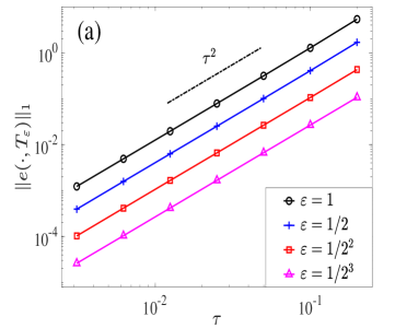
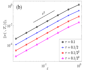
Figure 4.1. Temporal errors of the TSFP (2.31)–(2.32) for the NKGE (2.1) with $\beta=0$ for different $\varepsilon$ and $\tau$.

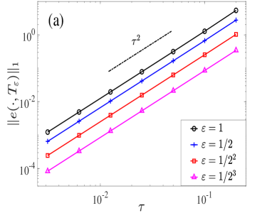
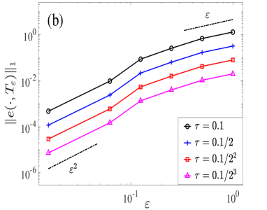
Figure 4.2. Temporal errors of the TSFP (2.31)–(2.32) for the NKGE (2.1) with $\beta=1$ for different $\varepsilon$ and $\tau$.

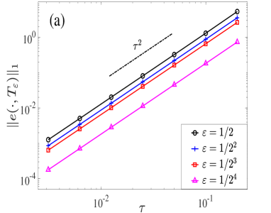
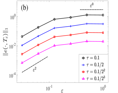
Figure 4.3. Temporal errors of the TSFP (2.31)–(2.32) for the NKGE (2.1) with $\beta=2$ for different $\varepsilon$ and $\tau$.

From Table 1 and Figures 4.1–4.3, we can draw the following observations:

(1) The TSFP method converges uniformly for $0<\varepsilon\leq 1$ in space with exponential convergence rate (cf. each row in Table 1).

(2) For any fixed $\varepsilon=\varepsilon_{0}>0$, the TSFP method (2.31)–(2.32) is second-order accurate in time (cf. each line in Figures 4.1(a)–4.3(a)). When $\beta=0$, the temporal error behaves like $O(\varepsilon^{2}\tau^{2})$ (cf. Figure 4.1(b)), which agrees with the theoretical result in Theorem 3.2. Figure 4.2(b) and Figure 4.3(b) show that the temporal error is at $O(\varepsilon\tau^{2})$ and $O(\tau^{2})$ for $\beta=1$ and $\beta=2$, respectively.

(3) Our numerical results confirm the uniform error bounds in Theorem 3.2.

Table 2. Comparison of the properties of the TSFP method (2.31)–(2.32) for the NKGE (1.1) at different long-time dynamics regimes with $T_{0}$ and $\tau_{0}$ are fixed and independent of $0<\varepsilon\leq 1$.

	$O(1)$-time with $\beta=0$	intermediate long-time with $0<\beta\leq\frac{p}{3}$	long-time with $\frac{p}{3}<\beta<p$	super long-time with $\beta=p$
final time $T_{\varepsilon}=\frac{T_{0}}{\varepsilon^{\beta}}$	$O(1)$	long-time $O(\varepsilon^{-\beta})$	longer-time $O(\varepsilon^{-\beta})$	longest-time $O(\varepsilon^{-p})$
largest time step size $\tau_{\varepsilon}=\tau_{0}\varepsilon^{\frac{\beta-p}{2}}$	largest time step size at $O(\varepsilon^{-p/2})$	larger time  step size at $O(\varepsilon^{\frac{\beta-p}{2}})$	large time  step size at $O(\varepsilon^{\frac{\beta-p}{2}})$	$O(1)$
total time steps $N_{\varepsilon}=\frac{T_{\varepsilon}}{\tau_{\varepsilon}}=\frac{T_{0}}{\tau_{0}}\varepsilon^{\frac{p-3\beta}{2}}$	$O(1)$	$O(1)$	$O(\varepsilon^{\frac{p-3\beta}{2}})$	$O(\varepsilon^{-p})$
total computational cost	$O(N\ln N)$	$O(N\ln N)$	$O(\varepsilon^{\frac{p-3\beta}{2}}N\ln N)$	$O(\varepsilon^{-p}N\ln N)$
spatial error	uniform spectral	uniform spectral	uniform spectral	uniform spectral
temporal error in term of $\tau_{0}$	uniform second-order	uniform second-order	uniform second-order	uniform second-order

We remark here that, when $0<\varepsilon\ll 1$, our numerical results suggest a better error bound as (cf. left-bottom parts in Figures 4.2(b)–4.3(b))

$$\|u(\cdot,t_{n})-I_{N}(u^{n})\|_{s}\lesssim h^{1+m-s}+\varepsilon^{p}\tau^{2},\quad 0\leq n\leq\frac{T_{0}/\varepsilon^{\beta}}{\tau}.$$

We emphasized this improved convergence when $\varepsilon\ll 1$ is missing for the EWI-FP method presented in [32], which shows the superiority of the TSFP method.

For convenience of readers, Table 2 summarizes the properties of the TSFP method (2.31)–(2.32) for the NKGE (1.1) at different long-time dynamics regimes.

5. Extension to an oscillatory complex NKGE in the whole space

In this section, we begin with a complex NKGE in the whole space, re-scale it into an oscillatory complex NKGE, compare properties of the NKGE under different scalings and extend the TSFP method and its error bounds to the oscillatory complex NKGE.

5.1. Comparisons of the complex NKGE under different scalings

Consider the following complex NKGE with a power-type nonlinearity in the whole space $\mathbb{R}^{d}$ ($d=1,2,3$) as

(5.1) $$\left\{\begin{aligned} &\partial_{tt}u({\bm{x}},t)-\Delta u({\bm{x}},t)+u({\bm{x}},t)+\varepsilon^{p}|u({\bm{x}},t)|^{p}u({\bm{x}},t)=0,\quad{\bm{x}}\in\mathbb{R}^{d},\quad t>0,\\ &u({\bm{x}},0)=u_{0}({\bm{x}})=O(1),\quad\partial_{t}u({\bm{x}},0)=u_{1}({\bm{x}})=O(1),\quad{\bm{x}}\in\mathbb{R}^{d}.\end{aligned}\right.$$

Here, $u:=u(\bm{x},t)$ is a complex-valued scalar field, and the initial datum $u_{0}({\bm{x}})$ and $u_{1}({\bm{x}})$ are two given complex-valued functions which are independent of the parameter $\varepsilon$. Again formally, the amplitude of the solution $u$ is at $O(1)$. The local/global well-posedness of the Cauchy problem (5.1) and scattering properties have been extensively studied in a considerable literature [34, 37, 38, 41, 48, 45, 49, 51]. Particularly, under appropriate assumptions on $p$, $d$, $\varepsilon$ and the initial conditions, the solutions of (5.1) are global [17] and scatter as $|t|\rightarrow\infty$ for small initial values (low energy scattering) [38, 45], or for all initial values (asymptotic completeness) [48, 49]. In addition, under proper regularity of the solution, the complex NKGE (5.1) is time symmetric or time reversible and conserves the energy [5, 6, 26] as

$$E_{1}(t) :=E_{1}(u(\cdot,t))=\int_{\mathbb{R}^{d}}\left[|\partial_{t}u(\bm{x},t)|^{2}+|\nabla u(\bm{x},t)|^{2}+|u(\bm{x},t)|^{2}+\frac{2\varepsilon^{p}}{p+2}|u(\bm{x},t)|^{p+2}\right]d\bm{x}$$

(5.2) $$\equiv\int_{\mathbb{R}^{d}}\left[|u_{1}(\bm{x})|^{2}+|\nabla u_{0}(\bm{x})|^{2}+|u_{0}(\bm{x})|^{2}+\frac{2\varepsilon^{p}}{p+2}|u_{0}(\bm{x})|^{p+2}\right]d\bm{x}$$

$$=E_{1}(0)=O(1),\qquad t\geq 0.$$

Plugging the plane wave solution $u(\bm{x},t)=Ae^{i(\bm{\xi}\cdot{\bm{x}}-\omega_{1}t)}$ (with $A$ the amplitude, $\bm{\xi}$ the spatial wave number and $\omega_{1}:=\omega_{1}(\bm{\xi})$ the time frequency) into the complex NKGE (5.1), we get the dispersion relation:

(5.3) $$\omega_{1}=\omega_{1}({\bm{\xi}})=\pm\sqrt{1+|{\bm{\xi}}|^{2}+\varepsilon^{p}A^{p}}=O(1),\quad\varepsilon\in(0,1],\quad\mathrm{for\,\,\,fixed}\,\,\,\bm{\xi}\in\mathbb{R}^{d},$$

which immediately implies the group velocity

(5.4) $$\bm{v}_{1}:=\bm{v}_{1}(\xi)=\nabla\omega_{1}(\bm{\xi})=\pm\frac{\bm{\xi}}{\sqrt{1+|\bm{\xi}|^{2}+\varepsilon^{p}A^{p}}}=O(1).$$

Thus the solution of the complex NKGE (5.1) propagates waves with amplitude at $O(1)$, wavelength in space and time at $O(1)$ and wave velocity at $O(1)$.

By introducing $w({\bm{x}},t)=\varepsilon u({\bm{x}},t)$, we can reformulate the complex NKGE (5.1) with weak nonlinearity (and initial data with amplitude at $O(1)$) into the following complex NKGE with small initial data (and $O(1)$ nonlinearity):

(5.5) $$\left\{\begin{aligned} &\partial_{tt}w({\bm{x}},t)-\Delta w({\bm{x}},t)+w({\bm{x}},t)+|w({\bm{x}},t)|^{p}w({\bm{x}},t)=0,\quad\bm{x}\in\mathbb{R}^{d},\quad t>0,\\ &w({\bm{x}},0)=\varepsilon u_{0}({\bm{x}})=O(\varepsilon),\quad\partial_{t}w({\bm{x}},0)=\varepsilon u_{1}({\bm{x}})=O(\varepsilon),\quad{\bm{x}}\in\mathbb{R}^{d}.\end{aligned}\right.$$

Noticing that the amplitude of the initial data in (5.5) is at $O(\varepsilon)$, formally we can get the amplitude of the solution $w$ of (5.5) is at $O(\varepsilon)$, too. Similarly, the complex NKGE (5.5) is time symmetric or time reversible and conserves the energy [5, 6, 26] as

$$E_{2}(t) :=E_{2}(w(\cdot,t))=\int_{\mathbb{R}^{d}}\big{[}|\partial_{t}w(\bm{x},t)|^{2}+|\nabla w(\bm{x},t)|^{2}+|w(\bm{x},t)|^{2}+\frac{2}{p+2}|w(\bm{x},t)|^{p+2}\big{]}d\bm{x}$$

$$\equiv\varepsilon^{2}\int_{\mathbb{R}^{d}}\left[|u_{1}(\bm{x})|^{2}+|\nabla u_{0}(\bm{x})|^{2}+|u_{0}(\bm{x})|^{2}+\frac{2\varepsilon^{p}}{p+2}|u_{0}(\bm{x})|^{p+2}\right]d\bm{x}$$

$$=E_{2}(0)=\varepsilon^{2}E_{1}(0)=O(\varepsilon^{2}),\qquad t\geq 0.$$

In addition, plugging the plane wave solution $w(\bm{x},t)=\varepsilon Ae^{i(\bm{\xi}\cdot{\bm{x}}-\omega_{1}t)}$ into the complex NKGE (5.5), we get the same dispersion relation (5.3) and the same group velocity (5.4) of the complex NKGE (5.5), i.e., the complex NKGEs (5.5) and (5.1) share the same dispersion relation (5.3) and the same group velocity (5.4). Again, the solution of the complex NKGE (5.5) propagates waves with amplitude at $O(\varepsilon)$, wavelength in space and time at $O(1)$ and wave velocity at $O(1)$.

Introducing a re-scale in time

(5.6) $$t=\frac{s}{\varepsilon^{\beta}}\Leftrightarrow s=\varepsilon^{\beta}t,\qquad\nu(\bm{x},s)=u(\bm{x},t),$$

with $0<\beta\leq p$ fixed, we can re-formulate the complex NKGE (5.1) into the following oscillatory complex NKGE

(5.7) $$\left\{\begin{split}&\partial_{ss}\nu(\bm{x},s)+\frac{1}{\varepsilon^{2\beta}}(-\Delta+1)\nu(\bm{x},s)+\varepsilon^{p-2\beta}|\nu(\bm{x},s)|^{p}\nu(\bm{x},s)=0,\,\,\,\,\bm{x}\in\mathbb{R}^{d},\,\,\,\,s>0,\\ &\nu(\bm{x},0)=u_{0}(\bm{x})=O(1),\quad\partial_{s}\nu(\bm{x},0)={\varepsilon}^{-\beta}u_{1}(\bm{x})=O({\varepsilon}^{-\beta}),\quad\bm{x}\in\mathbb{R}^{d}.\end{split}\right.$$

Formally, the amplitude of the solution $\nu$ of the oscillatory complex NKGE (5.7) is at $O(1)$. Again, the oscillatory complex NKGE (5.7) is time symmetric or time reversible and conserves the energy [5, 6, 26] as

$$E_{3}(s) :=E_{3}(\nu(\cdot,s))=\int_{\mathbb{R}^{d}}\left[|\partial_{s}\nu|^{2}+\frac{1}{\varepsilon^{2\beta}}\left(|\nabla\nu|^{2}+|\nu|^{2}\right)+\frac{2\varepsilon^{p-2\beta}}{p+2}|\nu|^{p+2}\right]d\bm{x}$$

(5.8) $$\equiv\frac{1}{\varepsilon^{2\beta}}\int_{\mathbb{R}^{d}}\left[|u_{1}(\bm{x})|^{2}+|\nabla u_{0}(\bm{x})|^{2}+|u_{0}(\bm{x})|^{2}+\frac{2\varepsilon^{p}}{p+2}|u_{0}(\bm{x})|^{p+2}\right]d\bm{x}$$

$$=E_{3}(0)=\varepsilon^{-2\beta}E_{1}(0)=O(\varepsilon^{-2\beta}),\qquad s\geq 0.$$

Again, plugging the plane wave solution $\nu(\bm{x},s)=Ae^{i(\bm{\xi}\cdot{\bm{x}}-\omega_{2}s)}$ (with $A$ the amplitude, $\bm{\xi}$ the spatial wave number and $\omega_{2}:=\omega_{2}(\bm{\xi})$ the time frequency) into the oscillatory complex NKGE (5.7), we get the dispersion relation:

(5.9) $$\omega_{2}=\omega_{2}(\bm{\xi})=\pm\frac{1}{\varepsilon^{\beta}}\sqrt{1+|\bm{\xi}|^{2}+\varepsilon^{p}A^{p}}=O(\varepsilon^{-\beta}),\qquad\bm{\xi}\in\mathbb{R}^{d},$$

which immediately implies the group velocity

(5.10) $$\bm{v}_{2}:=\bm{v}_{2}(\bm{\xi})=\nabla\omega_{2}(\bm{\xi})=\pm\frac{\bm{\xi}}{\varepsilon^{\beta}\sqrt{1+|\bm{\xi}|^{2}+\varepsilon^{p}A^{p}}}=O(\varepsilon^{-\beta}).$$

Thus the solution of the oscillatory complex NKGE (5.7) propagates waves with amplitude at $O(1)$, wavelength in space and time at $O(1)$ and $O(\varepsilon^{\beta})$, respectively, and wave velocity at $O(\varepsilon^{-\beta})$.

Remark 5.1.

We remark here that the above scalings of the complex NKGE are different from the following complex NKGE in the nonrelativistic regime, which has been widely used and studied in the literature [4, 5, 12, 10, 11, 46, 53]:

(5.11) $$\left\{\begin{aligned} &\partial_{tt}u({\bm{x}},t)-\frac{1}{\varepsilon^{2}}\Delta u({\bm{x}},t)+\frac{1}{\varepsilon^{4}}u({\bm{x}},t)+\frac{1}{\varepsilon^{2}}|u({\bm{x}},t)|^{2}u({\bm{x}},t)=0,\quad t>0,\\ &u({\bm{x}},0)=u_{0}({\bm{x}})=O(1),\quad\partial_{t}u({\bm{x}},0)=\varepsilon^{-2}u_{1}({\bm{x}})=O(\varepsilon^{-2}),\quad{\bm{x}}\in\mathbb{R}^{d}.\end{aligned}\right.$$

The above complex NKGE conserves the energy [5, 6, 26] as

$$E_{4}(t) :=E_{4}(u(\cdot,t))=\int_{\mathbb{R}^{d}}\Big{[}|\partial_{t}u(\bm{x},t)|^{2}+\frac{|\nabla u(\bm{x},t)|^{2}}{\varepsilon^{2}}+\frac{1}{\varepsilon^{4}}|u(\bm{x},t)|^{2}+\frac{1}{2\varepsilon^{2}}|u(\bm{x},t)|^{4}\Big{]}d\bm{x}$$

(5.12) $$\equiv\frac{1}{\varepsilon^{4}}\int_{\mathbb{R}^{d}}\left[|u_{1}(\bm{x})|^{2}+\varepsilon^{2}|\nabla u_{0}(\bm{x})|^{2}+|u_{0}(\bm{x})|^{2}+\frac{\varepsilon^{2}}{2}|u_{0}(\bm{x})|^{4}\right]d\bm{x}$$

$$=E_{5}(0)=O(\varepsilon^{-4}),\qquad t\geq 0.$$

Plugging the plane wave solution $u(\bm{x},t)=Ae^{i(\bm{\xi}\cdot{\bm{x}}-\omega_{3}t)}$ into the complex NKGE (5.11), we get the dispersion relation:

(5.13) $$\omega_{3}=\omega_{3}(\bm{\xi})=\pm\frac{1}{\varepsilon^{2}}\sqrt{1+\varepsilon^{2}|\bm{\xi}|^{2}+\varepsilon^{2}A^{2}}=O(\varepsilon^{-2}),\qquad\bm{\xi}\in\mathbb{R}^{d},$$

which immediately implies the group velocity

(5.14) $$\bm{v}_{3}:=\bm{v}_{3}(\bm{\xi})=\nabla\omega_{3}(\bm{\xi})=\pm\frac{\bm{\xi}}{\sqrt{1+\varepsilon^{2}|\bm{\xi}|^{2}+\varepsilon^{2}A^{2}}}=O(1).$$

Thus the solution of the complex NKGE (5.11) propagates waves with amplitude at $O(1)$, wavelength in space and time at $O(1)$ and $O(\varepsilon^{2})$, respectively, and wave velocity at $O(1)$.

For convenience of readers, Table 3 shows the properties of the complex NKGE under different scalings.

Table 3. Comparison of the complex NKGE under different scalings.

  (5.1) (5.5) (5.7) (5.11) amplitude $O(1)$ $O(\varepsilon)$ $O(1)$ $O(1)$ wavelength in space $O(1)$ $O(1)$ $O(1)$ $O(1)$ wavelength in time $O(1)$ $O(1)$ $O(\varepsilon^{\beta})$ $O(\varepsilon^{2})$ wave velocity $O(1)$ $O(1)$ $O(\varepsilon^{-\beta})$ $O(1)$ energy $O(1)$ $O(\varepsilon^{2})$ $O(\varepsilon^{-2\beta})$ $O(\varepsilon^{-4})$  

5.2. The TSFP method for the complex NKGE (5.7) and main results

Similar to those in the literature, we truncate the oscillatory complex NKGE (5.7) in 1D onto a bounded interval $\Omega=(a,b)$ with periodic boundary conditions as

(5.15) $$\left\{\begin{split}&\partial_{ss}\nu(x,s)+\frac{1}{\varepsilon^{2\beta}}(-\partial_{xx}+1)\nu(x,s)+\varepsilon^{p-2\beta}|\nu(x,s)|^{p}\nu(x,s)=0,\,\,\,s>0,\\ &\nu(a,t)=\nu(b,t),\quad\partial_{x}\nu(a,t)=\partial_{x}\nu(b,t),\qquad t\geq 0,\\ &\nu(x,0)=u_{0}(x),\quad\partial_{s}\nu(x,0)=\varepsilon^{-\beta}u_{1}(x),\quad x\in\overline{\Omega}=[a,b].\end{split}\right.$$

Denote $q(x,s)=\partial_{s}\nu(x,s)$, by taking $k=\varepsilon^{\beta}\tau$ and assuming $u_{0}$ and $u_{1}$ to be real-valued in (5.15), the TSFP discretization can be similarly obtained via (2.31). Under the following reasonable assumptions on the exact solution $\nu$ of the oscillatory NKGE (5.15)

$${\rm(B)}\begin{split}&\nu\in\ L^{\infty}\left([0,T_{0}];H^{m+1}_{\rm per}\right),\qquad\partial_{s}\nu\in L^{\infty}\left([0,T_{0}];H^{m}_{\rm per}\right),\\ &\|\nu\|_{L^{\infty}\left([0,T_{0}];H^{m+1}_{\rm per}\right)}\lesssim 1,\qquad\,\,\,\,\|\partial_{s}\nu\|_{L^{\infty}\left([0,T_{0}];H^{m}_{\rm per}\right)}\lesssim\frac{1}{\varepsilon^{\beta}},\end{split}$$

with $m\geq 1$, we can establish the following error bounds of the TSFP method for the oscillatory complex NKGE (5.15) (the proof is omitted here for brevity).

Theorem 5.2.

Let $\nu^{n}$, $q^{n}$ be the numerical approximation obtained from the TSFP method. Under the assumption (B), there exist $h_{0}>0$ and $k_{0}>0$ sufficiently small and independent of $\varepsilon$ such that, for any $0<\varepsilon\leq 1$, when $0<h\leq h_{0}$ and $0<k\leq k_{0}\varepsilon^{\frac{3\beta-p}{2}}$, we have the error estimates for $l\in(1/2,m]$

$$\|\nu(\cdot,s_{n})-I_{N}(\nu^{n})\|_{l}+\varepsilon^{\beta}\|\partial_{s}\nu(\cdot,s_{n})-I_{N}(q^{n})\|_{l-1}\lesssim h^{1+m-l}+\varepsilon^{p-3\beta}k^{2},\quad 0\leq n\leq\frac{T_{0}}{k}.$$

Remark 5.3.

From Theorem 5.2, we clearly see that the TSFP is uniformly second-order accurate in the weakly oscillatory case, i.e., $0\leq\beta\leq\frac{p}{3}$. Furthermore, large time step size at $k\sim\varepsilon^{\frac{3\beta-p}{2}}$ is allowed in practical computation when $0\leq\beta<\frac{p}{3}$. While for $\beta\in(\frac{p}{3},p]$, the TSFP method fails to be uniformly convergent and tiny time step is required as $k\lesssim\varepsilon^{\frac{3\beta-p}{2}}$.

5.3. Numerical results

In order to verify the error bounds in Theorem 5.2, we take $d=1$ and $p=3$ in (5.7) and the initial data

(5.16) $$u_{0}(x)=(2+i)e^{-x^{2}/2},\quad u_{1}(x)=\,{\mathrm{sech}}(x^{2}),\quad x\in\mathbb{R}.$$

The problem is solved on a bounded interval $\Omega_{\varepsilon}=[-8-\varepsilon^{-\beta},8+\varepsilon^{-\beta}]$ since the wave velocity is at $O(\varepsilon^{-\beta})$, which is large enough to guarantee that the periodic boundary condition does not introduce a significant truncation error relative to the original problem. The ‘exact’ solution $v(x,s)$ is obtained numerically by using the TSFP method with a fine mesh size $h_{e}=1/16$ and a very small time step $k_{e}={10}^{-5}$. We also measure the $H^{1}$-norm and the errors are displayed at $T_{0}=1$ with different $\varepsilon$ and $\beta$. For the oscillatory complex NKGE (5.7), we study the following three cases:

Case I. Weakly oscillatory regime, i.e., $\beta=1$;

Case II. Intermediate oscillatory regime, i.e., $\beta=2$;

Case III. Highly oscillatory regime, i.e., $\beta=3$.

For spatial error analysis, we fix the time step as $k={10}^{-5}$ such that the temporal errors can be neglected; for temporal error analysis, a very fine mesh size $h=1/16$ is chosen such that the spatial error can be ignored. Table 4 shows the spatial errors under different mesh size for these three cases and Tables 5-7 depict the temporal errors for $\beta=1,2,3$, respectively. In order to quantify the error, we introduce

$$e_{\infty}(t):=\max_{0<\varepsilon\leq 1}\{\|e(\cdot,t)\|_{1}\}.$$

Table 4. Spatial errors of the TSFP method for the oscillatory complex NKGE (5.15) with (5.16) for different $\beta$ and $\varepsilon$.

  $\|e(\cdot,1)\|_{1}$ $h_{0}=1$ $h_{0}/2$ $h_{0}/2^{2}$ $h_{0}/2^{3}$ $\beta=1$ $\varepsilon_{0}=1/2$ 1.57E-1 2.40E-3 5.82E-6 1.77E-9 $\varepsilon_{0}/2^{1}$ 9.52E-2 2.91E-3 8.47E-6 2.59E-10 $\varepsilon_{0}/2^{2}$ 5.85E-2 3.31E-3 1.11E-5 3.32E-10 $\varepsilon_{0}/2^{3}$ 1.03E-1 1.63E-3 1.18E-5 4.10E-10 $\beta=2$ $\varepsilon_{0}=1/2$ 2.01E-1 3.24E-3 1.02E-5 1.52E-9 $\varepsilon_{0}/2^{1}$ 1.11E-1 1.64E-3 1.19E-5 4.34E-10 $\varepsilon_{0}/2^{2}$ 1.28E-1 3.57E-3 1.55E-5 1.61E-10 $\varepsilon_{0}/2^{3}$ 1.18E-1 3.81E-3 1.34E-5 2.21E-10 $\beta=3$ $\varepsilon_{0}=1/2$ 1.91E-1 3.90E-3 1.40E-5 6.95E-9 $\varepsilon_{0}/2^{1}$ 1.55E-1 3.43E-3 1.58E-5 1.66E-10 $\varepsilon_{0}/2^{2}$ 1.30E-1 5.79E-3 5.94E-6 4.32E-10 $\varepsilon_{0}/2^{3}$ 1.25E-1 5.15E-3 1.59E-5 5.95E-10  

Table 5. Temporal errors of the TSFP method for the oscillatory complex NKGE (5.15) with (5.16) and $\beta=1$.

  $\|e(\cdot,1)\|_{1}$ $k_{0}=0.1$ $k_{0}/2$ $k_{0}/2^{2}$ $k_{0}/2^{3}$ $k_{0}/2^{4}$ $k_{0}/2^{5}$ $k_{0}/2^{6}$ $\varepsilon_{0}=1$ 2.82E-1 6.71E-2 1.66E-2 4.13E-3 1.03E-3 2.58E-4 6.45E-5 order - 2.07 2.02 2.01 2.00 2.00 2.00 $\varepsilon_{0}/2$ 1.15E-1 2.77E-2 6.85E-3 1.71E-3 4.27E-3 1.07E-4 2.67E-5 order - 2.05 2.02 2.00 2.00 2.00 2.00 $\varepsilon_{0}/2^{2}$ 4.20E-2 9.45E-3 2.31E-3 5.75E-4 1.43E-4 3.58E-5 8.96E-6 order - 2.15 2.03 2.01 2.01 2.00 2.00 $\varepsilon_{0}/2^{3}$ 4.91E-2 6.43E-3 1.46E-3 3.57E-4 8.89E-5 2.22E-5 5.54E-6 order - 2.93 2.14 2.03 2.01 2.00 2.00 $\varepsilon_{0}/2^{4}$ 2.29E-2 8.02E-3 1.01E-3 2.29E-4 5.60E-5 1.39E-5 3.48E-6 order - 1.51 2.99 2.14 2.03 2.01 2.00 $\varepsilon_{0}/2^{5}$ 8.77E-3 3.48E-3 1.21E-3 1.51E-4 3.43E-5 8.40E-6 2.09E-6 order - 1.33 1.52 3.00 2.14 2.03 2.01 $\varepsilon_{0}/2^{6}$ 9.87E-4 1.25E-3 4.88E-4 1.70E-4 2.10E-5 4.78E-6 1.17E-6 order - -0.34 1.36 1.52 3.02 2.14 2.03 $e_{\infty}(t=1)$ 2.82E-1 6.71E-2 1.66E-2 4.13E-3 1.03E-3 2.58E-4 6.45E-5 order - 2.07 2.02 2.01 2.00 2.00 2.00  

Table 6. Temporal errors of the TSFP method for the oscillatory complex NKGE (5.15) with (5.16) and $\beta=2$.

  $\|e(\cdot,1)\|_{1}$ $k_{0}=0.1$ $k_{0}/2$ $k_{0}/2^{2}$ $k_{0}/2^{3}$ $k_{0}/2^{4}$ $k_{0}/2^{5}$ $\varepsilon_{0}=1$ 2.82E-1 6.71E-2 1.66E-2 4.13E-3 1.03E-3 2.58E-4 order - 2.07 2.02 2.01 2.00 2.00 $\varepsilon_{0}/4^{1/3}$ 5.15E-1 1.14E-1 2.77E-2 6.89E-3 1.72E-3 4.30E-4 order - 2.18 2.04 2.01 2.00 2.00 $\varepsilon_{0}/4^{2/3}$ 1.52 2.20E-1 5.08E-2 1.25E-2 3.11E-3 7.76E-4 order - 2.79 2.11 2.02 2.01 2.00 $\varepsilon_{0}/4$ 1.40 6.80E-1 8.95E-2 2.03E-2 4.96E-3 1.23E-3 order - 1.04 2.93 2.14 2.03 2.01 $\varepsilon_{0}/4^{4/3}$ 9.33E-1 6.94E-1 3.18E-1 3.88E-2 8.11E-3 1.96E-3 order - 0.43 1.13 3.03 2.26 2.05 $\varepsilon_{0}/4^{5/3}$ 3.10E-1 2.48E-1 2.85E-1 1.19E-1 2.07E-2 3.45E-3 order - 0.32 -0.20 1.26 2.52 2.58  

Table 7. Temporal errors of the TSFP method for the oscillatory complex NKGE (5.15) with (5.16) and $\beta=3$.

  $\|e(\cdot,1)\|_{1}$ $k_{0}=0.1$ $k_{0}/4$ $k_{0}/4^{2}$ $k_{0}/4^{3}$ $k_{0}/4^{4}$ $k_{0}/4^{5}$ $\varepsilon_{0}=1$ 2.82E-1 1.66E-2 1.03E-3 6.45E-5 4.03E-6 2.50E-7 order - 2.04 2.01 2.00 2.00 2.01 $\varepsilon_{0}/4^{1/3}$ 3.82 1.34E-1 8.23E-3 5.14E-4 3.21E-5 1.99E-6 order - 2.42 2.01 2.00 2.00 2.01 $\varepsilon_{0}/4^{2/3}$ 8.46 6.37E-1 3.35E-2 2.08E-3 1.30E-4 8.03E-6 order - 1.87 2.12 2.00 2.00 2.01 $\varepsilon_{0}/4$ 4.08 1.95 1.22E-1 6.76E-3 4.20E-4 2.60E-5 order - 0.53 2.00 2.09 2.00 2.01 $\varepsilon_{0}/4^{4/3}$ 1.39 1.15 5.40E-1 2.61E-2 1.45E-3 8.92E-5 order - 0.14 0.55 2.19 2.08 2.01 $\varepsilon_{0}/4^{5/3}$ 4.26E-1 3.59E-1 2.98E-1 1.39E-1 6.17E-3 3.40E-4 order - 0.12 0.13 0.55 2.25 2.09  

From Tables 4-6 and additional similar results not shown here for brevity, we can draw the following observations for the TSFP method:

(1) The TSFP method is uniformly and spectrally accurate in space for any $0\leq\beta\leq p$ (cf. Table 4).

(2) When $\beta=1$, the TSFP method converges quadratically in time, which is uniformly for $0<\varepsilon\leq 1$ (cf. last row in Table 5). While for cases $\beta=2$ and $\beta=3$, second-order convergence can only be observed when $k\lesssim\varepsilon^{3/2}$ and $k\lesssim\varepsilon^{3}$, respectively (cf. the upper triangle above the main diagonal in Tables 6-7). This agrees with the analytical result in Theorem 5.2.

(3) For $\beta=2$ and $\beta=3$, when $0<\varepsilon\ll 1$ and $k\lesssim\varepsilon^{\frac{3\beta-p}{2}}$, Tables 6–7 suggest the following improved error bound

$$\|v(\cdot,s_{n})-I_{N}(v^{n})\|_{l}\lesssim h^{1+m-l}+\varepsilon^{p-2\beta}k^{2},\quad 0\leq n\leq T_{0}/k.$$

Again, for convenience of readers, Table 8 summarizes the properties of the TSFP method for the oscillatory NKGE (5.7) at different parameter regimes.

Table 8. Comparison of the properties of the TSFP method for the oscillatory NKGE (5.15) at different parameter regimes, while $T_{0}$ and $k_{0}$ are fixed and independent of $0<\varepsilon\leq 1$.

	$\beta=0$	$0<\beta<\frac{p}{3}$	$\beta=\frac{p}{3}$	$\frac{p}{3}<\beta<\frac{p}{2}$	$\beta=\frac{p}{2}$	$\frac{p}{2}<\beta\leq p$
nonlinearity strength $\varepsilon^{p-2\beta}$	weakest $O(\varepsilon^{p})$	weaker $O(\varepsilon^{p-2\beta})$	weak $O(\varepsilon^{p/3})$	weak $O(\varepsilon^{p-2\beta})$	$O(1)$	strong $O(\varepsilon^{p-2\beta})$
time step size $k_{\varepsilon}=k_{0}\varepsilon^{\frac{3\beta-p}{2}}$	larger $O(\varepsilon^{-p/2})$	large $O(\varepsilon^{\frac{3\beta-p}{2}})$	$O(1)$	small $O(\varepsilon^{\frac{3\beta-p}{2}})$	smaller $O(\varepsilon^{p/4})$	smallest $O(\varepsilon^{\frac{3\beta-p}{2}})$
total time steps $N_{\varepsilon}=\frac{T_{0}}{k_{\varepsilon}}=\frac{T_{0}}{k_{0}}\varepsilon^{\frac{p-3\beta}{2}}$	$O(1)$	$O(1)$	$O(1)$	many steps at $O(\varepsilon^{\frac{p-3\beta}{2}})$	many steps at $O(\varepsilon^{-\frac{p}{4}})$	many steps at $O(\varepsilon^{\frac{p-3\beta}{2}})$
total cost	$O(N\ln N)$	$O(N\ln N)$	$O(N\ln N)$	$O\left(\frac{N\ln N}{\varepsilon^{\frac{3\beta-p}{2}}}\right)$	$O\left(\varepsilon^{\frac{p}{4}}N\ln N\right)$	$O\left(\frac{N\ln N}{\varepsilon^{\frac{3\beta-p}{2}}}\right)$
spatial error	uniform spectral	uniform spectral	uniform spectral	uniform spectral	uniform spectral	uniform spectral
temporal error	uniform	uniform	uniform	non-uniform	non-uniform	non-uniform

6. Conclusion

An efficient and accurate time-splitting Fourier pseudospectral (TSFP) method was proposed and analyzed for the long-time dynamics of the nonlinear Klein–Gordon equation (NKGE) with weak nonlinearity or small initial data. Uniform error bounds of the TSFP method were established up to the time at $O(\varepsilon^{-p})$ with $0<\varepsilon\leq 1$ a dimensionless parameter used to characterize the nonlinearity strength. Numerical results were reported to confirm our error bounds in the long-time regime. Extension of the method and its error bounds to an oscillatory complex NKGE in the whole space was discussed.

References

- [1] W. Bao and Y. Cai, Mathematical theory and numerical methods for Bose-Einstein condensation, Kinet. Relat. Models 6 (2013), no. 1, 1–135.
- [2] W. Bao, Y. Cai, X. Jia, and Q. Tang, Numerical methods and comparison for the Dirac equation in the nonrelativistic limit regime, J. Sci. Comput. 71 (2017), no. 3, 1094–1134.
- [3] W. Bao, Y. Cai, X. Jia, and J. Yin, Error estimates of numerical methods for the nonlinear Dirac equation in the nonrelativistic limit regime, Sci. China Math. 59 (2016), no. 8, 1461–1494.
- [4] W. Bao, Y. Cai, and X. Zhao, A uniformly accurate multiscale time integrator pseudospectral method for the Klein–Gordon equation in the nonrelativistic limit regime, SIAM J. Numer. Anal. 52 (2014), no. 5, 2488–2511.
- [5] W. Bao and X. Dong, Analysis and comparison of numerical methods for the Klein–Gordon equation in the nonrelativistic limit regime, Numer. Math. 120 (2012), no. 2, 189–229.
- [6] W. Bao, Y. Feng, and W. Yi, Long time error analysis of finite difference time domain methods for the nonlinear Klein-Gordon equation with weak nonlinearity, Commun. Comput. Phys. 26 (2019), no. 5, 1307–1334.
- [7] W. Bao, S. Jin, and P. A. Markowich, Numerical study of time-splitting spectral discretizations of nonlinear Schrödinger equations in the semiclassical regimes, SIAM J. Sci. Comput. 25 (2003), no. 1, 27–64.
- [8] W. Bao and J. Shen, A fourth-order time-splitting Laguerre–Hermite pseudospectral method for Bose–Einstein condensates, SIAM J. Sci. Comput. 26 (2005), no. 6, 2010–2028.
- [9] W. Bao and C. Su, A uniformly and optimally accurate method for the Zakharov system in the subsonic limit regime, SIAM J. Sci. Comput. 40 (2018), no. 2, A929–A953.
- [10] W. Bao and X. Zhao, Comparison of numerical methods for the nonlinear Klein–Gordon equation in the nonrelativistic limit regime, J. Comput. Phys. 398 (2019), article 108886.
- [11] S. Baumstark, E. Faou, and K. Schratz, Uniformly accurate exponential-type integrators for Klein-Gordon equations with asymptotic convergence to the classical NLS splitting, Math. Comp. 87 (2018), no. 311, 1227–1254.
- [12] P. Bechouche, N. J. Mauser, and S. Selberg, Nonrelativistic limit of Klein-Gordon-Maxwell to Schrödinger-Poisson, Amer. J. Math. 126 (2004), no. 1, 31–64.
- [13] J. Bernier, E. Faou, and B. Grébert, Long time behavior of the solutions of NLW on the d-dimensional torus, Forum Math. Sigma, 8 (2020), 12.
- [14] J. Bourgain, Construction of approximative and almost periodic solutions of perturbed linear Schrödinger and wave equations, Geom. Funct. Anal. 6 (1996), no. 2, 201–230.
- [15] P. Brenner and W. von Wahl, Global classical solutions of nonlinear wave equations, Math. Z. 176 (1981), no. 1, 87–121.
- [16] R. Carles and C. Gallo, On Fourier time-splitting methods for nonlinear Schrödinger equations in the semi-classical limit II. Analytic regularity, Numer. Math. 136 (2017), no. 1, 315–342.
- [17] T. Cazenave and I. Naumkin, Local smooth solutions of the nonlinear Klein-Gordon equation, Discrete Cont. Dyn. Syst. S 14 (2021), no. 5, 1649–1672.
- [18] P. Chartier, N. Crouseilles, M. Lemou, and F. Méhats, Uniformly accurate numerical schemes for highly oscillatory Klein–Gordon and nonlinear Schrödinger equations, Numer. Math. 129 (2015), no. 2, 211–250.
- [19] P. Chartier, F., Méhats, M. Thalhammer, and Y. Zhang, Improved error estimates for splitting methods applied to highly-oscillatory nonlinear Schrödinger equations, Math. Comp. 85 (2016), no. 302, 2863–2885.
- [20] S. C. Chikwendu and C. V. Easwaran, Multiple-scale solution of initial-boundary value problems for weakly nonlinear wave equations on the semi-infinite line, SIAM J. Appl. Math. 52 (1992), no. 4, 946–958.
- [21] D. Cohen, E. Hairer, and C. Lubich, Conservation of energy, momentum and actions in numerical discretizations of nonlinear wave equations, Numer. Math. 110 (2008), no. 2, 113–143.
- [22] D. Cohen, E. Hairer, and C. Lubich, Long-time analysis of nonlinearly perturbed wave equations via modulated Fourier expansions, Arch. Rat. Mech. Anal. 187 (2008), no. 2, 341–368.
- [23] J.-M. Delort, Temps d’existence pour l’équation de Klein-Gordon semi-linéaire à données petites périodiques, Amer. J. Math. 120 (1998), no. 3, 663–689.
- [24] J.-M. Delort, On long time existence for small solutions of semi-linear Klein-Gordon equations on the torus, J. Anal. Math. 107 (2009), no. 1, 161–194.
- [25] J.-M. Delort and J. Szeftel, Long time existence for small data nonlinear Klein-Gordon equations on tori and spheres, Int. Math. Res. Not. IMRN 2004 (2004), no. 37, 1897–1966.
- [26] X. Dong, Z. Xu, and X. Zhao, On time-splitting pseudospectral discretization for nonlinear Klein-Gordon equation in nonrelativistic limit regime, Commun. Comput. Phys. 16 (2014), no. 2, 440–466.
- [27] D. B. Duncan, Symplectic finite difference approximations of the nonlinear Klein–Gordon equation, SIAM J. Numer. Anal. 34 (1997), no. 5, 1742–1760.
- [28] M. Faccioli and L. Salasnich, Spontaneous symmetry breaking and Higgs mode: comparing Gross-Pitaevskii and nonlinear Klein-Gordon equations, Symmetry, 10 (2018), no. 4, 80.
- [29] D. Fang and Q. Zhang, Long-time existence for semi-linear Klein–Gordon equations on tori, J. Differential Equations 249 (2010), no. 1, 151–179.
- [30] E. Faou and K. Schratz, Asymptotic preserving schemes for the Klein–Gordon equation in the non-relativistic limit regime, Numer. Math. 126 (2014), no. 3, 441–469.
- [31] Y. Feng, Long time error analysis of the fourth-order compact finite difference methods for the nonlinear Klein-Gordon equation with weak nonlinearity, Numer. Methods Partial Differential Equations 37 (2021), no. 1, 897–914.
- [32] Y. Feng and W. Yi, Uniform error bounds of an exponential wave integrator Fourier pseudospectral method for the long-time dynamics of the nonlinear Klein-Gordon equation, Multiscale Model. Simul. 19 (2021), no. 3, 1212 – 1235.
- [33] H. Feshbach and F. Villars, Elementary relativistic wave mechanics of spin 0 and spin 1/2 particles, Rev. Modern Phys. 30 (1958), no. 1, 24–45.
- [34] J. Ginibre and G. Velo, The global Cauchy problem for the non linear Klein-Gordon equation, Math Z. 189 (1985), no. 4, 487–505.
- [35] E. Hairer and C. Lubich, Spectral semi-discretizations of weakly non-linear wave equations over long times, Found. Comput. Math. 8 (2008), no. 3, 319–334.
- [36] Z. Huang, S. Jin, P. A. Markowich, C. Sparber, and C. Zheng, A time-splitting spectral scheme for the Maxwell–Dirac system, J. Comput. Phys. 208 (2005), no, 2, 761–789.
- [37] M. Keel and T. Tao, Small data blow-up for semilinear Klein-Gordon equations, Amer. J. Math. 121 (1999), no. 3, 629–669.
- [38] S. Klainerman, Global existence of small amplitude solutions to nonlinear Klein-Gordon equations in four space-time dimensions, Comm. Pure Appl. Math. 38 (1985), no. 5, 631–641.
- [39] V. V. Konotop, A. Sànchez, and L. Vàzquez, Kink dynamics in the weakly stochastic model, Phys. Rev. B 44 (1991), no. 6, 2554-2566.
- [40] P. S. Landa, Nonlinear Oscillations and Waves in Dynamical Systems, Kluwer Academic Publishers, Boston, MA, 1996.
- [41] H. J. Landau, Necessary density conditions for sampling and interpolation of certain entire functions, Acta Math. 117 (1967), no. 1, 37–52.
- [42] K. Li and Q. Zhang, Existence and nonexistence of global solutions for the equation of dislocation of crystals, J. Differential Equations 146 (1998), no. 1, 5–21.
- [43] H. Lindblad, On the lifespan of solutions of nonlinear wave equations with small initial data, Comm. Pure Appl. Math. 43 (1990), no. 4, 445–472.
- [44] C. Lubich, On splitting methods for Schrödinger-Poisson and cubic nonlinear Schrödinger equations, Math. Comp. 77 (2008), no. 264, 2141–2153.
- [45] S. Masaki and J. Segata, Modified scattering for the quadratic nonlinear Klein–Gordon equation in two dimensions, Trans. Amer. Math. Soc. 370 (2018), no. 11, 8155–8170.
- [46] N. Masmoudi and K. Nakanishi, From nonlinear Klein-Gordon equation to a system of coupled nonlinear Schrödinger equations, Math. Ann. 324 (2002), no. 2, 359–389.
- [47] R. I. McLachlan, and G. R. W. Quispel, Splitting methods, Acta Numer., 11 (2002), 341–434.
- [48] C. S. Morawetz and W. A. Strauss, Decay and scattering of solutions of a nonlinear relativistic wave equation, Comm. Pure Appl. Math. 25 (1972), no. 1, 1–31.
- [49] K. Nakanishi, Energy scattering for nonlinear Klein–Gordon and Schrödinger equations in spatial dimensions 1 and 2, J. Funct. Anal. 169 (1999), no. 1, 201–225.
- [50] K. Ono, Global existence and asymptotic behavior of small solutions for semilinear dissipative wave equations, Discrete Cont. Dyn. Syst. 9 (2003), no. 3, 651–662.
- [51] T. Ozawa, K. Tsutaya, and Y. Tsutsumi, Global existence and asymptotic behavior of solutions for the Klein-Gordon equations with quadratic nonlinearity in two space dimensions, Math. Z. 222 (1996), no. 3, 341–362.
- [52] J. J. Sakurai, Advanced Quantum Mechanics, Addison-Wesley, New York, 1967.
- [53] A. Y. Schoene, On the nonrelativistic limits of the Klein–Gordon and Dirac equations, J. Math. Anal. Appl. 71 (1979), no. 1, 36–47.
- [54] C. E. Shannon, A mathematical theory of communication, Bell Syst. Tech. J. 27 (1948), 379–423, 623–656.
- [55] J. Shen and T. Tang, Spectral and High-Order Methods with Applications, Science Press, Beijing, 2006.
- [56] J. Shen and Z. Wang, Error analysis of the Strang time-splitting Laguerre–Hermite/Hermite collocation methods for the Gross–Pitaevskii equation, Found. Comput. Math. 13 (2013), no. 1, 99–137.
- [57] W. Strauss and L. Vázquez, Numerical solution of a nonlinear Klein–Gordon equation, J. Comput. Phys. 28 (1978), no. 2, 271–278.
- [58] C. Su and X. Zhao, On time-splitting methods for nonlinear Schrödinger equation with highly oscillatory potential, ESAIM: Math. Model. Numer. Anal. 54 (2020), no. 5, 1491–1508.
- [59] W. von Wahl, Regular solutions of initial-boundary value problems for linear and nonlinear wave-equations II, Math. Z. 142 (1975), no. 2, 121–130.
- [60] A. M. Wazwaz, The tanh and the sine–cosine methods for compact and noncompact solutions of the nonlinear Klein–Gordon equation, Appl. Math. Comput. 167 (2005), no. 2, 1179–1195.
- [61] W. Yi, X. Ruan and C. Su, Optimal resolution methods for the Klein–Gordon–Dirac system in the nonrelativistic limit regime, J. Sci. Comput. 79 (2019), no. 3, 1907–1935.