Identifying trending coefficients with an ensemble Kalman filter

Abstract

This paper extends the ensemble Kalman filter (EnKF) for inverse problems to identify trending model coefficients. This is done by repeatedly inflating the ensemble while maintaining the mean of the particles. As a benchmark serves a classic EnKF and a recursive least squares (RLS) on the example of identifying a force model in milling, which changes due to the progression of tool wear. For a proper comparison, the true values are simulated and augmented with white Gaussian noise. The results demonstrate the feasibility of the approach for dynamic identification while still achieving good accuracy in the static case. Further, the inflated EnKF shows a remarkably insensitivity on the starting set but a less smooth convergence compared to the classic EnKF.

1 Introduction

In milling, a rotating cutting movement is overlaid with a translatory feed movement resulting in an cyclically intermittent cutting process. It is a flexible and highly dynamic manufacturing process for free-form surfaces. This leads to a continuously varying thickness of the removed chip and with it a varying force.

The force is the most important parameter to analyze and evaluate the cutting process. Ever since there were machine tools, researchers aimed at describing the force through models in order to better understand and design the process. Nowadays, those models are also used for advanced control of the milling process, be it adaptive control (Altintas and Aslan, 2017) or even model-based predictive control (MPC) (Stemmler et al., 2017). The semi-empirical models must be calibrated for every tool-workpiece material combination. They represent a certain tool state and change as the tool wears. Historically, the identification was conducted off-line but new approaches have paved the way for an on-line identification in the manufacturing process.
This work discusses the problem of identifying changing coefficients. For this a constrained EnKF is repeatedly inflated and benchmarked against a RLS. The overall objective is to present a method for continuous identification of time-variant models.

2 State of the art

2.1 Force model

So-called mechanistic models relate the force to the cross-section of the undeformed chip. The most popular examples are the exponential force model according to Kienzle (1952) and the linear approach according to Altintas and Lee (1996):

$$F_{i,Kienzle} =k_{i}\,b\,h^{1-m_{i}}\hskip 28.45274pt i\in t,r,$$ (1)

$$F_{i,Altintas} =b\,\left(K_{i,e}+K_{i,c}\,h\right) i\in t,r.$$ (2)

The parameters $k_{i}$ and $m_{i}$, or $K_{i,e}$ and $K_{i,c}$ respectively, represent material-specific coefficients. The indices $i=t,r$ indicate the tangential and the radial component of the force vector. The undeformed chip thickness $h$ and the undeformed chip width $b$ form the cross-section of the chip.

Often, the admissibility range of linear models is extended by assuming the coefficients to be themselves again a function of the undeformed chip thickness $h$, e.g. as a linear (Grossi, 2017), an exponential (Wan et al., 2007, 2009; Campatelli and Scippa, 2012; Zhang et al., 2018), or a polynomial relation (Wei et al., 2018; Wang et al., 2018). This converts the linear model with varying coefficients $K=f(h)$ into a non-linear – often exponential – model with constant coefficients (Wan et al., 2007; Yao et al., 2013).

2.2 Model identification

The great majority of the work on how to identify the coefficients of mechanistic force models has been done for linear models, namely the force model of Altintas (Eq. 2). Few works identify a non-linear force model (Jayaram et al., 2001; Dotcheva et al., 2008; Wang et al., 2013; Adem et al., 2015; Zhang et al., 2017b, 2018) or the Kienzle-model explicitly (Shin and Waters, 1997; Perez et al., 2013; Schwenzer et al., 2018).

There exist two ways to identify such mechanistic force models in milling: the method of average force and the method of instantaneous undeformed chip thickness. The first is inspired from turning where the chip geometry does not vary resulting in a static cutting force. In milling this is approximated by averaging the dynamic force signal over a revolution. The method requires several dedicated experiments and is not on-line capable.
The method of instantaneous undeformed chip thickness is essentially a curve fit between measurements and a simulated force signal. They have been dominated by global optimization, such as evolutionary algorithms (Grossi, 2017; Chen et al., 2018), or particle swarm algorithms (Zhang et al., 2017b) for both presented models (Eq. 1, Eq. 2). Nevertheless, local optimization algorithms have a significant advantage in computation with no loss in accuracy (Freiburg et al., 2015; Schwenzer et al., 2018).

Adem et al. (2015) compared both models and identification methods. They concluded that a non-linear force model is generally more accurate than a linear model and that the optimization-based curve fit results in more accurate models than the average forces approach. Gonzalo et al. (2010) focused on the latter comparing identification methods. They define a “true” reference by identifying the coefficients in turning. Though the improvement is small, they argue that the method of instantaneous undeformed chip thickness has a better physical credibility due to the correspondence to the turning coefficients.

First studies on a continuous formulation of the method of instantaneous undeformed chip thickness propose an EnKF as a non-linear estimator to identify the Kienzle-model (Schwenzer et al., 2019b, a). The studies revealed the extraordinary insensitivity of the EnKF to measurement noise. They used an unscaled version of the filter as a trade-off for fast convergence against stability.

3 Approach

Progressive tool wear changes the model coefficients gradually. Therefore, we examine the case of trending coefficients as a special case of changing coefficients. For this, we suggest three different approaches for a continuous identification of a time-varying model:

• RLS,

• classic EnKF,

• EnKF with repeated ensemble inflation (EnKF^⋆).

In order to meet generality, we use the non-linear Kienzle-model, which is in fact not observable. Neither the RLS, nor the EnKF require observability of the system as they do not demand uniqueness of the solution of the inverse problem.

3.1 Recursive least square

The RLS algorithm is a least square fit taking the estimate of the previous time instance into account. It works as similar to an exponential smoothing with a decreased weighting of the previous information.

Assume an arbitrary measurement system

$$\hat{\bm{y}}_{k} =f(\hat{\bm{x}}_{k})\approx\bm{M}_{k}^{\intercal}\,\hat{\bm{x}}_{k}\text{,}$$ (3)

with a measurement $\hat{\bm{y}}_{k}$ that has non-linear relationship to the estimated state vector $\hat{\bm{x}}_{k}$ for time instance $k$ (Strejc, 1979). For a proper state-space representation, the relationship is linearized through the measurement-matrix $\bm{M}_{k}^{\intercal}$. The model-matrix weights the error between the measurement and the prediction through the gain $\bm{G}_{k}$

$$\hat{\bm{x}}_{k} =\hat{\bm{x}}_{k-1}+\bm{G}_{k}\,\left(\bm{z}_{k}-f(\hat{\bm{x}}_{k})\right),$$ (4)

$$\bm{G}_{k} =\frac{\bm{P}_{k-1}\,\bm{M}_{k}}{\rho+\bm{M}_{k}^{\intercal}\,\bm{P}_{k-1}\,\bm{M}_{k}},$$ (5)

$$\bm{P}_{k} =\frac{1}{\rho}\,\left[\bm{I}-\bm{G}_{k}\,\bm{M}_{k}^{\intercal}\right]\,\bm{P}_{k-1}.$$ (6)

The recursive approximation of the covariance matrix $\bm{P}_{k}$ limits the computational complexity. In the case on hand, the state vector becomes $\hat{\bm{x}}_{k}=\left[k_{i}\quad m_{i}\right]^{\intercal}$. The forgetting factor $0<\rho\leq 1$ (here $\rho=0.98$) weights the samples. The initial value of the covariance matrix is set to $\bm{P}_{0}=10^{5}\,\bm{I}$, with the identity matrix $\bm{I}$. Applying this to

3.2 Ensemble Kalman filter

Instead of integrating a single state vector forward in time, the EnKF propagates an ensemble of state vectors and takes its mean as the best-guess (Evensen, 1994). The backbone of the EnKF is a Markov chain Monte Carlo simulation of the evolution in time of individual state vectors, which approximate the true probability density of the states (Evensen, 2003). The EnKF is a special case of a particle filter without re-sampling and with Gaussian distribution for the measurement likelihood.

Assuming an ensemble matrix

$$\bm{X}_{k|k-1}=(\bm{x}_{k|k-1}^{1},\dots,\bm{x}_{k|k-1}^{J}),$$ (7)

with $J$ individual state vectors $\bm{x}_{k|k-1}^{j},\ j\in\{1,\dots,J\}$ at time step $k$ based on the information from time step $k-1$. In the case on hand, the state vector is

$$\bm{x}$$ = [ ,

(8)

consisting out of the measurable forces $F_{i}$ and the non-observable parameters $k_{i}$, $m_{i}$. The RLS does not require the measurements to be a member of the state vector.

The EnKF is a truly non-linear estimator, using the model function $f(\bm{x},\bm{u})$ to propagate every member of the ensemble forward in time based on the current input $\bm{u}_{k}$:

$$\hat{\bm{X}}_{k|k-1} =f\left(\bm{X}_{k-1|k-1},\bm{u}_{k}\right),$$ (9)

$$\bm{P}_{k|k-1} =\frac{1}{J}~{}(\hat{\bm{X}}_{k|k-1}-\overline{\bm{X}}_{k|k-1})\,(\hat{\bm{X}}_{k|k-1}-\overline{\bm{X}}_{k|k-1})^{\intercal}.$$ (10)

The error covariance matrix is approximated by the empirical covariance matrix of the ensemble $\bm{P}$. It represents the spread to the mean of the ensemble $\overline{\bm{X}}$. Recent studies (Schwenzer et al., 2019b, a) resign from scaling the covariance $\bm{P}$, which favors the convergence speed but comes at the cost of a higher instability. The unscaled version of the filter looses the feature of mathematical well-posedness, that is why it is not further considered.

The predicted state vectors are updated through the measurements weighted by the Kalman gain $\bm{G}_{k}$:

$$\bm{G}_{k} =\bm{P}_{k|k-1}\,\bm{H}_{k}^{\intercal}~{}\left[\bm{H}_{k}\,\bm{P}_{k|k-1}\,\bm{H}_{k}^{\intercal}+\overline{\bm{R}}_{k}\right]^{-1},$$ (11)

$$\bm{x}_{k|k}^{j} =\hat{\bm{x}}_{k|k-1}^{j}+\bm{G}_{k}\left[\bm{z}_{k}^{j}-\bm{H}_{k}\,\hat{\bm{x}}_{k|k-1}^{j}\right]$$ (12)

where $\bm{H}_{k}$ is the linear observation operator and the single measurement vector $\bm{y}_{k}$ is augmented with artificial zero-mean Gaussian noise $\bm{\varepsilon}\sim\mathcal{N}(\bm{0},\,\bm{\Gamma})$:

$$\bm{z}_{k}^{j} =\bm{y}_{k}+\bm{\varepsilon}_{k}^{j},\qquad j\in\{1,\dots,J\}$$ (13)

$$\bm{Z}_{k} =\left(\bm{z}_{k}^{1},\dots,\bm{z}_{k}^{n}\right)^{\intercal},\quad\text{and}$$ (14)

$$\overline{\bm{R}}_{k} =\frac{1}{J}\,\left(\bm{\varepsilon}_{k}\,\bm{\varepsilon}_{k}^{\intercal}\right).$$ (15)

The update of the empirical covariance matrix $\bm{P}_{k|k}$ is calculated as before, but now uses the information of the current time step $k$

$$\bm{P}_{k|k} =\frac{1}{J}\,(\bm{X}_{k|k}-\overline{\bm{X}}_{k|k})\,(\bm{X}_{k|k}-\overline{\bm{X}}_{k|k})^{\intercal}.$$ (16)

Note that the Kalman gain $\bm{G}_{k}$, Eq. 11, and the covariances $\bm{P}_{k|k-1}$, Eq. 10, and $\bm{P}_{k|k}$, Eq. 16, are the same for all ensemble members and only need to be calculated once.

In the case of application to inverse problems, the EnKF can be written in the following formulation

$$\bm{X}_{k+1|k+1}= \bm{X}_{k|k}+\bm{C}_{k|k}\,\left(\bm{D}_{k|k}+\bm{\Gamma}\right)^{-1}\,\left(\bm{Z}_{k+1}-\hat{\bm{Y}}_{k}\right),$$ (17)

$$\bm{C}_{k|k}= \frac{1}{J}(\hat{\bm{Y}}_{k}-\overline{\hat{\bm{Y}}}_{k})\,(\hat{\bm{Y}}_{k}-\overline{\hat{\bm{Y}}}_{k})^{\intercal},$$ (18)

$$\bm{D}_{k|k}= \frac{1}{J}(\bm{X}_{k|k}-\overline{\bm{X}}_{k|k})\,(\hat{\bm{Y}}_{k}-\overline{\hat{\bm{Y}}}_{k})^{\intercal},$$ (19)

which is often used in the field of mathematics in order to analyse the general behavior of the filter and to provide a comprehensive theoretical background. Whereas often the measurements $\bm{y}_{k}$ are not augmented: $\bm{\varepsilon}_{k}=\bm{0}\Rightarrow\bm{Z}_{k}=\bm{y}_{k}$. This facilitates the analysis of the stability and well-posedness of the EnKF. However, perturbing the measurements creates individual observations for every member and prevents particles from synchronizing and collapsing completely to a potentially non-optimal solution (Kelly et al., 2014).

Although the filter converges within the subspace spanned by the initial ensemble – i.e. the mean value of the ensemble converges to a value within this subset – it is not guaranteed that all ensemble members stay within this subset at all times. This makes it fragile if the model used is not defined for all states or exhibits singularities.
Enforcing box constraints, hoping that the particular member does not get saturated but will (eventually) move back into the subspace some time, is reasonable if the initial ensemble is chosen properly. That is if the solution lays within the limits, so that the whole ensemble is drawn towards its mean by the common covariance. Further, if the ensemble is large enough, it is unlikely that many members are affected by artificial box constraints and; thus, distort the expected behavior of the filter. In fact, Chada et al. (2019) showed that the EnKF can impose box-constraints by projecting states that violate a constraint back onto the boundary (this is the projected Newton method). This might affect the convergence because it changes the direction and the step-size of the particle. Considering the EnKF as a sequential optimization, it becomes obvious that the optimization gets affected. Nevertheless, it is still ensured that the ensembles collapse to their mean and that the method converges to a Karush-Kuhn-Tucker (KKT) point of the optimization problem.

In the case of identifying mechanistic force models in milling, the box-constraints for the state vector $\bm{x}$ were set to

$$\bm{x}_{lb}$$ = [ 500 100 0.1 0.1 ,

= [ 3500 2100 1 1 .

(20)

3.3 Ensemble Kalman filter with repeated ensemble inflation

The problem of identifying time-variant models could be approached by restarting the EnKF if the model accuracy runs out of bound. This would neglect all prior gained information and reset the filter. In contrast to restarting the EnKF over and over again, the ensemble inflation should maintain the current mean $\overline{\bm{X}}_{k}^{\star}\approx\overline{\bm{X}}_{k}$ but be brought back to the initial spread, i.e. covariance $\bm{P}_{0}$.

On a regular basis, the ensemble $\hat{\bm{X}}_{k}$ is substituted by an ensemble $\hat{\bm{X}}_{k}^{\star}$ with the covariance

$$\bm{P}_{k|k}^{\star}=\frac{1}{\lambda}\,\bm{P}_{0}$$ (21)

In contrast to this, variance inflation scales the covariance ahead of the analysis, Eq. 11 or Eq. 17 respectively. It keeps the particles from collapsing too fast, which is of importance at problems of high dimensions (large number of states) and a comparatively small ensemble size.
Ensemble inflation replaces the complete ensemble in discrete steps after analysis.

The idea of the mean field theory is that many small random subsets of particles on average represent the behavior of the whole particle cloud (Herty and Visconti, 2019). Following the mean field theory, we inflate only a small subset of the ensemble set $\bm{\mathcal{X}}\subset\{\bm{x}^{j}\}_{j=1}^{J}$, $|\bm{\mathcal{X}}|=M\ll J$, with regard to its mean. This should smooth the inflation or the immediate effect of the inflation respectively. The ensemble size was set to $J=100$ and the subset $M$ to $10\text{\,}\mathrm{\char 37\relax}$.

3.4 Simulation for validation

In general, three distinct cases must be considered for identification:

• static coefficients,

• ascending coefficients, and

• alternating coefficients.

For validation, this paper simulates 10 revolutions of a straight milling operation with a flat end-mill emulating a machining of stainless steel (X5CrNi18-10) with a two-fluted solid carbide tool, Tab. 1. Those are the same conditions as in (Schwenzer et al., 2019b, a) for reasons of consistency and a better comparison.

Table 1: Tool and process parameters

Tool geometry			Process parameter
Diameter	$D$	$10\text{\,}\mathrm{mm}$	Feed	$f$	$0.1\text{\,}\mathrm{mm}$
Number of teeth	$N_{z}$	2	Cutting velocity	$v_{c}$	$2.44\text{\,}\mathrm{m}\text{\,}{\mathrm{s}}^{-1}$
Helix angle	$\beta$		Depth of cut	$a_{p}$	$2\text{\,}\mathrm{mm}$
Rake angle	$\gamma$		Width of cut	$a_{e}$	$3\text{\,}\mathrm{mm}$

Since mechanistic force models are defined for straight cutting edges, the helix angle of the tool is approximated as a spiral staircase, in this case with 23 disk elements. The force measurements were simulated assuming the coefficients given in Tab. 2, which were taken from one of the most extensive work on coefficients of the Kienzle-model (König et al., 1982). Using a sample frequency of $f_{s}=$10\text{\,}\mathrm{kHz}$$, a revolution translates to approximately $234$ samples. Artificial Gaussian noise with signal-to-noise ratio (S/N) of 15 was added to the simulated force signals in order to mimic severe measurement noise. Fig. 1 illustrates the different cases and the added noise. Simulating the force signals allows to use the coordinate system of the cutting edge, in which the model is defined, and to evaluate if the identification tends towards the true coefficients.

Table 2: Force coefficients for the Kienzle force model for X5CrNi18-10

	$k_{t}$	$m_{t}$	$k_{r}$	$m_{r}$
upper bound	1800	0.6	1200	0.3
lower bound	800	0.05	600	0.01
X5CrNi18-10 (König et al., 1982, s. 95)	1700	0.18	350	0.55

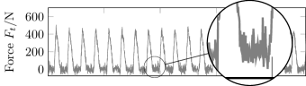
static ascending alternating

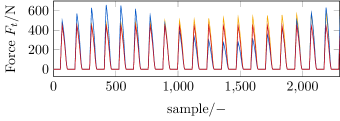
Figure 1: Simulated force signals: added white Gaussian noise with S/N = 15 for the static case (top); different cases without Gaussian noise (bottom)

The EnKF embraces randomness as it depends on the choice of the initial ensemble and of the random perturbations at every step. In order to perform a sensitivity analysis, the EnKF is restarted with $N_{init}=1000{}$ different initial ensembles for every simulation case. The initial ensembles were generated as a uniform random distribution within the boundaries given in Tab. 2. They were generated once beforehand and the pseudo-random generator is initialized to the same value for every simulation case. For the RLS, the mean of the initial ensemble served as the starting value.

When the undeformed chip thickness is tool small, cutting turns into ploughing and models loose their validity. Therefore, the identification was set to transit when the undeformed chip thickness (the sum along the disk elements) was smaller than a threshold $h_{TH}=$0.01\text{\,}\mathrm{mm}$$. Those corrected samples are denoted as samples^′.

For the sake of conciseness and without loss of generality, the discussion is limited to the tangential component of the force and the coefficients $i=t$. All calculations were performed with the software MATLAB R2018b from The MathWorks on an AMD Ryzen7-2700 ($3\text{\,}\mathrm{GHz}$) computer running Windows 10.

4 Results and discussion

From a grid-search we learned that large steps and a small inflation (large $\lambda$) are better for slowly changing model coefficients; while small steps and a large inflation is required for dynamic and drastic changes, Tab. 3. Though this finding is intuitive, it is difficult to choose the optimal parameters. A good compromise were small steps and a small inflation because the increase in accuracy for quasi-static problems is much smaller than the loss in accuracy for a dynamic problem. Therefore, the step-size, in which the ensemble is inflated, was set to 50 samples^′ and the inflation factor to $\lambda=10$.

Table 3: Root-mean-square of the error, Eq. 22, for different inflation steps and fractions

Method	step	$\lambda$	static	ascending	alternating
EnKF⋆	50	1.5	7.6	8.4	8.5
EnKF⋆	50	1	7.8	8.6	8.6
EnKF⋆	50	10	6.4	7.2	8.9
EnKF⋆	50	2	7.5	8.3	8.5
EnKF⋆	50	5	6.9	7.7	8.4
EnKF⋆	100	1.5	6.5	7.2	11.9
EnKF⋆	100	1	6.6	7.3	11.5
EnKF⋆	100	10	5.6	6.6	14.1
EnKF⋆	100	2	6.4	7.1	12.2
EnKF⋆	100	5	6.0	6.8	13.0
EnKF⋆	200	1.5	4.6	7.3	20.2
EnKF⋆	200	1	4.7	7.3	19.6
EnKF⋆	200	10	4.2	7.3	23.6
EnKF⋆	200	2	4.6	7.3	20.6
EnKF⋆	200	5	4.4	7.2	22.2
EnKF	$\infty$	-	3.8	23.2	50.7

Figure. 2 illustrates the evolution of the error for the different identification methods in all three cases. The transparent tubes indicate the variance within the 1000 simulations with different initial ensembles ($\overline{\Delta\bm{F}_{t}}\pm 2\,\sigma(\Delta\bm{F}_{t})$). That are $95.45\text{\,}\mathrm{\char 37\relax}$ if this Monte Carlo simulation is normally distributed. The error is defined as the difference in the force between the identified and the ideal coefficients

$$\Delta F_{t}=F_{t,sim}-F_{t,ideal}=\hat{k}_{t}\,b\,h^{1-\hat{m}_{t}}-k_{t}\,b\,h^{1-m_{t}}.$$ (22)

One can see that the RLS (yellow lines) hardly depends on the initial value. Therefrom, it is remarkable how drastic the variation of the mean became; in particular when identifying static coefficients. The error even ran out of the box and broke down in a singularity as no box-constraints were imposed. In general, the RLS exhibited a high oscillation in the mean error (thick lines) with no sign of convergence. Previous studies suggested that it is particularly prone to measurement noise (Schwenzer et al., 2019a).
The dynamic cases (“ascending” and “alternating”) revealed that the classic EnKF (blue lines) was not sufficient but only worked ideal in the case of static model coefficients. However, inflating the ensemble repeatedly (red) decreased the accuracy in the static case but was the only option to achieve accurate results for identifying trending coefficients. The samples where the ensemble was inflated are marked by the dotted grid-lines.

	RLS EnKF EnKF⋆
static
ascending
alternating

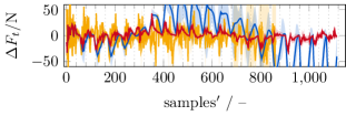
Figure 2: Evolution of the error in the tangential force $\Delta F_{t}$ with the Kienzle-model

Examining the evolution of the identified coefficients, Fig. 3, suggested an even worse performance of the RLS than by just considering the model error. It was not capable of following the trending coefficients. However, the EnKF seemed to follow the trend in the exponential coefficient $m_{t}$ quite well – perfectly in the case of the linear ascent. This might have been due to the comparatively small change, since the exponential model coefficient has a narrow range and a $20\text{\,}\mathrm{\char 37\relax}$ linear change did not require to maintain a large spread of the ensemble. However, it fails to follow the linearly ascending coefficient $k_{t}$ and revealed an extraordinary variance in the case of an alternating coefficient $k_{t}$ (light blue area). It appears that the changes are too drastic and too fast; in particular the alternating case of $k_{t}$ suggests a time-delay of the identification. The repeated inflation of the ensemble (abbreviated here as EnKF^⋆, red lines) shows a small variance tube. The filter follows the trending coefficients and still exhibits good convergence in the static case. In general, the EnKF^⋆ leads to an unsteady convergence, which becomes especially obvious in comparison to the classic EnKF in the static case.

	RLS EnKF EnKF⋆ original
static
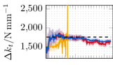
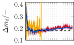
ascending
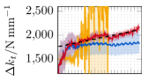
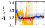
alternating

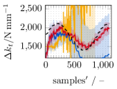
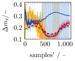
Figure 3: Evolution of the tangential coefficients of the Kienzle-model

5 Conclusion

A repeated inflation of (a subset of) the ensemble allows to identify time-varying coefficients. Instead of restarting the identification on a regular basis, the inflation maintains the ensemble mean as its current best-guess while enlarging the spread of the ensemble. This ensures that the ensemble explores the whole search-space at all times. Inflating the ensemble consistently changes the subspace; therefore, convergence within the initial ensemble cannot be guaranteed anymore. To regain control of the identification, it is important to impose box-constraints on the filter. Furthermore, the amount of inflation is set to a fraction of the variance of the initial ensemble to limit the spread. The fraction can be smaller the smaller the step-size of the ensemble inflation. As an idea from the mean-field theory, only a subset of the ensemble is inflated in order to smooth the continuous identification.

The results show that the classic EnKF is only able to follow trending coefficient in exceptional cases, i.e. slow and small changes and with a high sensitivity to the initial ensemble. A repeated inflation of the ensemble drastically reduced this sensitivity and presented the only option to follow all cases of trending coefficients. However, at the cost of a slightly worse accuracy in the static case compared to the classic EnKF. The RLS, which served as a benchmark, revealed an immense proneness to the artificial white Gaussian noise in the measurements.

Future research will be placed on the integrating the mean field theory to the EnKF in order to decrease oscillation and increasing stability through an adaptive time-step within the filter. In milling, identification of a time-varying force model must be combined with the quasi-static identification of a model of the radial deviation of the tool. Eventually, the application to real measurement signals remain due.

The authors would like to thank the German Research Foundation DFG for the kind support within the Cluster of Excellence “Internet of Production” (Project ID: 390621612).

References

- Adem et al. (2015) Adem, K.A.M., Fales, R., and El-Gizawy, A.S. (2015). Identification of cutting force coefficients for the linear and nonlinear force models in end milling process using average forces and optimization technique methods. The International Journal of Advanced Manufacturing Technology, 79(9-12), 1671–1687. 10.1007/s00170-015-6935-3.
- Altintas and Aslan (2017) Altintas, Y. and Aslan, D. (2017). Integration of virtual and on-line machining process control and monitoring. CIRP Annals - Manufacturing Technology, 66(1), 349–352. 10.1016/j.cirp.2017.04.047.
- Altintas and Lee (1996) Altintas, Y. and Lee, P. (1996). A General Mechanics and Dynamics Model for Helical End Mills. CIRP Annals - Manufacturing Technology, 45(1), 59–64. 10.1016/S0007-8506(07)63017-0.
- Campatelli and Scippa (2012) Campatelli, G. and Scippa, A. (2012). Prediction of Milling Cutting Force Coefficients for Aluminum 6082-T4. Procedia CIRP, 1, 563–568. 10.1016/j.procir.2012.04.100.
- Chada et al. (2019) Chada, N.K., Schillings, C., and Weissmann, S. (2019). On the Incorporation of Box-Constraints for Ensemble Kalman Inversion. arXiv:1908.00696 [cs, math]. ArXiv: 1908.00696.
- Chen et al. (2018) Chen, D., Zhang, X., Xie, Y., and Ding, H. (2018). Precise Estimation of Cutting Force Coefficients and Cutter Runout in Milling using Differential Evolution Algorithm. Procedia CIRP, 77, 283–286. 10.1016/j.procir.2018.09.016.
- Dotcheva et al. (2008) Dotcheva, M., Millward, H., and Lewis, A. (2008). The evaluation of cutting-force coefficients using surface error measurements. Journal of Materials Processing Technology, 196(1-3), 42–51. 10.1016/j.jmatprotec.2007.04.136.
- Evensen (1994) Evensen, G. (1994). Sequential data assimilation with a nonlinear quasi-geostrophic model using Monte Carlo methods to forecast error statistics. Journal of Geophysical Research, 99(C5), 10143. 10.1029/94JC00572.
- Evensen (2003) Evensen, G. (2003). The Ensemble Kalman Filter: theoretical formulation and practical implementation. Ocean Dynamics, 53(4), 343–367. 10.1007/s10236-003-0036-9.
- Freiburg et al. (2015) Freiburg, D., Hense, R., Kersting, P., and Biermann, D. (2015). Determination of Force Parameters for Milling Simulations by Combining Optimization and Simulation Techniques. Journal of Manufacturing Science and Engineering, 138(4), 044502. 10.1115/1.4031336.
- Gonzalo et al. (2010) Gonzalo, O., Beristain, J., Jauregi, H., and Sanz, C. (2010). A method for the identification of the specific force coefficients for mechanistic milling simulation. International Journal of Machine Tools and Manufacture, 50(9), 765–774. 10.1016/j.ijmachtools.2010.05.009.
- Grossi (2017) Grossi, N. (2017). Accurate and fast measurement of specific cutting force coefficients changing with spindle speed. International Journal of Precision Engineering and Manufacturing, 18(8), 1173–1180. 10.1007/s12541-017-0137-x.
- Herty and Visconti (2019) Herty, M. and Visconti, G. (2019). Kinetic Methods for Inverse Problems. Kinet. Relat. Models, 12(5), 1109–1130.
- Jayaram et al. (2001) Jayaram, S., Kapoor, S., and DeVor, R. (2001). Estimation of the specific cutting pressures for mechanistic cutting force models. International Journal of Machine Tools and Manufacture, 41(2), 265–281. 10.1016/S0890-6955(00)00076-6.
- Kelly et al. (2014) Kelly, D.T.B., Law, K.J.H., and Stuart, A.M. (2014). Well-posedness and accuracy of the ensemble Kalman filter in discrete and continuous time. Nonlinearity, 27(10), 2579–2603. 10.1088/0951-7715/27/10/2579.
- Kienzle (1952) Kienzle, O. (1952). Die Bestimmung von Kräften und Leistungen an spanenden Werkzeugmaschinen. In VDI-Z, volume 96 of VDI-Z, 299–305. VDI-Verlag. Eines Vortrages von Prof. O. Kienzle auf der 81. VDI-Hauptversammlung der Fachgruppe Betriebstechnik. Quelle: VDI-Z 96 (1952) 11-12, S. 299-305.
- König et al. (1982) König, W., Essel, K., Witte, L., and Verein Deutscher Eisenhüttenleute (1982). Spezifische Schnittkraftwerte für die Zerspanung metallischer Werkstoffe. Verlag Stahleisen, Düsseldorf. OCLC: 64323901.
- Perez et al. (2013) Perez, H., Diez, E., Marquez, J.J., and Vizan, A. (2013). An enhanced method for cutting force estimation in peripheral milling. The International Journal of Advanced Manufacturing Technology, 69(5-8), 1731–1741. 10.1007/s00170-013-5153-0.
- Schwenzer et al. (2018) Schwenzer, M., Auerbach, T., Döbbeler, B., and Bergs, T. (2018). Comparative study on optimization algorithms for online identification of an instantaneous force model in milling. The International Journal of Advanced Manufacturing Technology. 10.1007/s00170-018-3109-0.
- Schwenzer et al. (2019a) Schwenzer, M., Stemmler, S., Ay, M., Bergs, T., and Abel, D. (2019a). Continuous identification for mechanistic force models in milling. IFAC, Berlin. Not yet published.
- Schwenzer et al. (2019b) Schwenzer, M., Stemmler, S., Ay, M., Bergs, T., and Abel, D. (2019b). Ensemble Kalman filtering for force model identification in milling. Procedia CIRP, 82, 296–301. 10.1016/j.procir.2019.04.028.
- Shin and Waters (1997) Shin, Y.C. and Waters, A.J. (1997). A new procedure to determine instantaneous cutting force coefficients for machining force prediction. International Journal of Machine Tools and Manufacture, 37(9), 1337–1351. 10.1016/S0890-6955(96)00093-4.
- Stemmler et al. (2017) Stemmler, S., Abel, D., Schwenzer, M., Adams, O., and Klocke, F. (2017). Model Predictive Control for Force Control in Milling. IFAC-PapersOnLine, 50(1), 15871–15876. 10.1016/j.ifacol.2017.08.2336.
- Strejc (1979) Strejc, V. (1979). Least Squares Parameter Estimation. IFAC Proceedings Volumes, 12(8), 535–550. 10.1016/S1474-6670(17)53975-0.
- Wan et al. (2007) Wan, M., Zhang, W.H., Tan, G., and Qin, G.H. (2007). New algorithm for calibration of instantaneous cutting-force coefficients and radial run-out parameters in flat end milling. Proceedings of the Institution of Mechanical Engineers, Part B: Journal of Engineering Manufacture, 221(6), 1007–1019. 10.1243/09544054JEM515.
- Wan et al. (2009) Wan, M., Zhang, W.H., Dang, J.W., and Yang, Y. (2009). New procedures for calibration of instantaneous cutting force coefficients and cutter runout parameters in peripheral milling. International Journal of Machine Tools and Manufacture, 49(14), 1144–1151. 10.1016/j.ijmachtools.2009.08.005.
- Wang et al. (2013) Wang, B., Hao, H., Wang, M., Hou, J., and Feng, Y. (2013). Identification of instantaneous cutting force coefficients using surface error. The International Journal of Advanced Manufacturing Technology, 68(1-4), 701–709. 10.1007/s00170-013-4792-5.
- Wang et al. (2018) Wang, L., Si, H., Guan, L., and Liu, Z. (2018). Comparison of different polynomial functions for predicting cutting coefficients in the milling process. The International Journal of Advanced Manufacturing Technology, 94(5-8), 2961–2972. 10.1007/s00170-017-1086-3.
- Wei et al. (2018) Wei, Z.C., Guo, M.L., Wang, M.J., Li, S.Q., and Liu, S.X. (2018). Prediction of cutting force in five-axis flat-end milling. The International Journal of Advanced Manufacturing Technology. 10.1007/s00170-017-1380-0.
- Yao et al. (2013) Yao, Z.Q., Liang, X.G., Luo, L., and Hu, J. (2013). A chatter free calibration method for determining cutter runout and cutting force coefficients in ball-end milling. Journal of Materials Processing Technology, 213(9), 1575–1587. 10.1016/j.jmatprotec.2013.03.023.
- Zhang et al. (2018) Zhang, X., Zhang, J., Zhang, W., Li, J., and Zhao, W. (2018). A non-contact calibration method for cutter runout with spindle speed dependent effect and analysis of its influence on milling process. Precision Engineering, 51, 280–290. 10.1016/j.precisioneng.2017.08.020.
- Zhang et al. (2017a) Zhang, X., Zhang, W., Zhang, J., Pang, B., and Zhao, W. (2017a). General Modeling and Calibration Method for Cutting Force Prediction With Flat-End Cutter. Journal of Manufacturing Science and Engineering, 140(2), 021007. 10.1115/1.4038371.
- Zhang et al. (2017b) Zhang, Z., Li, H., Meng, G., Ren, S., and Zhou, J. (2017b). A new procedure for the prediction of the cutting forces in peripheral milling. The International Journal of Advanced Manufacturing Technology, 89(5-8), 1709–1715. 10.1007/s00170-016-9186-z.