Einselection from incompatible decoherence channels

Abstract

Decoherence of quantum systems from entanglement with an unmonitored environment is to date the most compelling explanation of the emergence of a classical picture from a quantum world. While it is well understood for a single Lindblad operator, the role in the einselection process of a complex system-environment interaction remains to be clarified. In this paper, we analyze an open quantum dynamics inspired by CQED experiments with two non-commuting Lindblad operators modeling decoherence in the number basis and dissipative decoherence in the coherent state basis. We study and solve exactly the problem using quantum trajectories and phase-space techniques. The einselection optimization problem, which we consider to be about finding states minimizing the variation of some entanglement witness at a given energy, is studied numerically. We show that Fock states remain the most robust states to decoherence up to a critical coupling.

I Introduction

The strangeness of the quantum world comes from the principle of superposition and entanglement. Explaining the absence of those characteristic features in the classical world is the key point of the quantum-to-classical transition problem. The fairly recent theoretical and experimental progresses have largely reshaped our understanding of the emergence of a classical world from quantum theory alone. Indeed, decoherence theory Zurek (2003) has greatly clarified how quantum coherence is apparently lost for an observer through the entanglement of the system with a large unmonitored environment. At the same time, this interaction with the environment allows to understand the emergence of specific classical pointer states, a process called einselection.

However, in the case of complex environments, the physics of decoherence can be much more involved. It is then necessary to consider the structure of the environment. A recent approach exploring this path, called quantum Darwinism Zurek (2008, 2009), considers an environment composed of elementary fragments accessing a partial information about the system. While a lot of insights were originally model-based Zwolak et al. (2009); Riedel and Zurek (2010, 2011); Riedel et al. (2012, 2016), it has been proved that some basic assumptions of the quantum Darwinism approach, like the existence of a common objective observable, come directly from the theoretical framework of quantum theory Brandão et al. (2015); Knott et al. (2018); Qi and Ranard (2020).

Another possible source of complexity comes from the possibility that the environment can measure different observables of the system. Formally, the effective dynamics of the system will be described by many Lindblad operators which may be non commuting. When right eigenvectors of a Lindblad operator exist, which correspond to exact pointer states, we say that the operator describes a decoherence channel. Non-commuting Lindblad operators will give rise to what we call incompatible decoherence channels Arthurs and Kelly (1965); Briegel and Englert (1993); Torres (2014); Torres et al. (2019). Interesting physical effects are coming from the subtle interplay between those incompatible channels. For instance, the physics of a quantum magnetic impurity in a magnetic medium can be modeled as an open quantum system problem in which the environment probes all three Pauli matrices, instead of only one as in the standard spin-boson model Neto et al. (2003); Novais et al. (2005). Depending on the relative values of the coupling constants, different classical regimes emerge at low energy with one channel dominating the others. What’s more, for some fine tuned cases, the more interesting phenomena of decoherence frustration occurs Novais et al. (2005) where all channels contribute to suppress the loss of coherence of the system at all energy scales. This kind of subtleties in the einselection process have also been studied in circuit QED Bonzom et al. (2008); Jordan and Büttiker (2005); Ruskov et al. (2010); Hacohen-Gourgy et al. (2016); Essig et al. (2020) where, once again, the emergent classical picture is strongly dependent on the structure of the environment and the relative strength of its decoherence channels.

Thus, in the case of several incompatible decoherence channels, the problem of the emergence of a privileged basis is far from trivial. In this paper, we analyze the einselection process of a system in contact with two competing decoherence channels inspired by cavity QED experiments. The system a mode of the electromagnetic field confined in a high-quality cavity. The two sources of decoherence, one in the coherent state family and the other in the number basis, comes for the imperfections of this cavity and the atoms used to probe the field that are sent through the cavity. We base our analysis on the Lindblad equation to describe the effective open quantum dynamics. The problem is solved exactly using the quantum trajectory, the characteristic function and the quantum channel approaches allowing to properly characterize the different parameter regimes. These methods allow to go beyond the formal solution Torres (2014); Torres et al. (2019) by offering a clearer physical representation of the dynamics and the relevant timescales of the the problem. Still, the einselection problem, which is about finding the most robust (approximate) states to the interaction with the environment, has to be solved numerically. We choose those states as the pure states that minimize the short-time variation of some entanglement witness (the purity) with the environment at a given fixed energy. Depending on the relative values of the coupling constant, we find the intuitive result that the einselected states interpolate between Fock and coherent states. However, we uncover the remarkable fact that Fock states remain exactly the optimal einselected states up to a critical value of the couplings that can be obtained analytically. Finally, in the long-term dynamics, the einselection process appears to be much more complicated.

The paper is structured as follows. In Section II, we present a summary of techniques to derive the reduced dynamics from the full system-environment unitary evolution. This section can be skipped if the reader accepts Eq. 4. The core results are presented in Section III where the model is solved exactly. The einselection process is analyzed in Section IV and we present numerical evaluation of the Wigner function of the system which are used to properly analyze the different einselection regimes. We conclude in Section V by discussing how our analysis could be generalized and understood from a more abstract perspective through the algebraic structure of the jump operators.

II Motivations from CQED

By managing to entangle a single mode of the electromagnetic field and an atom, cavity quantum electrodynamics (CQED) is a nice experimental setup to explore the foundations of quantum theory, quantum information and the physics of the quantum to classical transition.

One implementation of CQED Haroche and Raimond (2013) uses an electromagnetic mode trapped in high quality factor mirrors as a system which is probed by a train of atoms acting as two-level systems (qubits) conveniently prepared. The setup can work in different regimes where the qubit is in resonance or not with the field. The off-resonance functioning mode, also called the dispersive regime, is particularly interesting since the atoms can be thought as small transparent dielectric medium with respect to the field with an index of refraction depending on its state. The atom is able to register some phase information about the field making it a small measurement device. In fact, a train of atoms can be thought as a non-destructive measurement device probing the number of photons in the field. Focusing our attention on the field itself, the atoms have to be considered as part of the environment of the field (even if it is well controlled by the experimentalist) giving rise to a decoherence channel having the Fock states as pointer states Haroche and Raimond (2013); Nogues et al. (1999); Guerlin et al. (2007). Similar experiments can also now be performed on circuit QED platforms Essig et al. (2020).

However, a second source of decoherence exists, not controlled by the experimentalist this time, and has its origin in the imperfections of the cavity. Indeed, while the quality factor is high enough to see subtle quantum phenomenon, photons can still get lost over time in the remaining electromagnetic environment. This second decoherence channel leads to a decoherence of the field mode on the coherent state basis of the electromagnetic field Caldeira and Leggett (1985), and introduces dissipation.

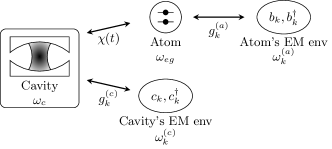
Figure 1: Dynamics of the cavity. The cavity is coupled to its own electromagnetic environment and to an atom, itself coupled to its own electromagnetic environment. We suppose that the two electromagnetic baths are not coupled. Eventually, the coupling of the cavity to its bath leads to photon losses. The coupling with the atom, in the dispersive regime, leads to decoherence on the photon basis.

We thus have two natural decoherence channels in this experimental setup, one which selects photon number states and the other coherent states. However, those two basis are incompatible in the sense that they are associated to complementary operators, the phase and number operators. This strong incompatibility between those classical states motivates the question on which classical pictures, if any, emerge from such a constrained dynamics.

Before analyzing this problem in details, let’s first put the previous discussion on firmer ground by deriving an open quantum system dynamics of the Lindblad form. We use a Born-Markov approximation of an effective Hamiltonian describing a CQED experiment represented on Fig. 1. As a starting point, consider the following Hamiltonian:

$$H =H_{S}+H_{E}+H_{SE}\,,$$ (1a)

$$H_{S} =\hbar\omega_{c}\,N\,,$$ (1b)

$$H_{E} =\frac{1}{2}\hbar\omega_{eg}\,\sigma_{z}+\sum_{k}\hbar\omega^{(c)}_{k}c^{\dagger}_{k}c_{k}+\sum_{k}\hbar\omega^{(a)}_{k}b^{\dagger}_{k}b_{k}$$

$$+\sigma_{z}\cdot\sum_{k}\hbar g^{(a)}_{k}(b^{\dagger}_{k}+b_{k})\,,$$ (1c)

$$H_{SE} =\hbar\chi(t)\,N\cdot\sigma_{z}+a\cdot\sum_{k}g^{(c)}_{k}c^{\dagger}_{k}+h.c.\,,$$ (1d)

with $(a,b,c)$ ladder operators of harmonic oscillators associated to the system and two environments respectively, $N=a^{\dagger}a$ the number operator for the system oscillator $a$ and $\sigma_{z}$ the $z$ Pauli matrix. The system of interest is the mode confined in the cavity. Its free Hamiltonian $H_{S}$ is just the free harmonic oscillator at frequency $\omega_{c}$. The cavity mode is coupled to two other systems:

1. The atom at frequency $\omega_{eg}$. It is coupled to the cavity in the dispersive regime defined as a non zero dephasing $\Delta=\omega_{eg}-\omega_{c}$ between the qubit and the cavity. This is the first term of $H_{SE}$. The coupling constant $\chi(t)$ is given by $g^{2}(t)/4\Delta$ where $g(t)$ is the coupling constant in the Jaynes-Cummings model. This atom is subjected to an electromagnetic environment described by the harmonic modes $(\omega^{(a)}_{k},g^{(a)}_{k})$ coupled to it by a spin-boson model. Both the atom and its electromagnetic environment form the first decoherence channel.

2. Other harmonic modes $\omega^{(c)}_{k}$ describing the electromagnetic environment of the cavity. In the secular approximation, this environment leads to photon losses in the cavity. This is the second decoherence channel.

The first decoherence channel is given by the atom passing through the cavity. Its effect on the field is characterized by a correlation function of the form:

$$G^{(a)}_{\rho}(t,t^{\prime})=\langle\chi(t)\sigma_{z}(t)\,\chi(t^{\prime})\sigma_{z}(t^{\prime})\rangle_{\rho}=\chi(t)\chi(t^{\prime})\,.$$ (2)

We remark that, in this case, the correlation function is independent of the state of the qubit $\rho$. We will rewrite the correlation function in terms of the variable $\tau=t-t^{\prime}$. Supposing that $G^{(a)}_{\rho}(t,t^{\prime})$ satisfies the usual assumptions of the Born-Markov approximation scheme (stationnarity and fast decay), the operators appearing in the Born-Markov equation are of the form $\int_{0}^{+\infty}G^{(a)}(t,\tau)\,\mathrm{e}^{-\mathrm{i}\omega\tau}\,\mathrm{d}\tau\,N$. From there follows a Lindblad equation with the jump operator $L_{n}(\omega)=\sqrt{2G^{(a)}(-\omega)}N$. Unfortunately, it is not possible to satisfy those requirement for the function $\chi(t)$ (indeed, stationarity implies that $\chi$ should be a phase but, being real, it must be a constant which cannot satisfy the decay requirement). Thus, the time dependence must be kept in full generality in this model, breaking the usual stationarity assumption. This is not a problem for the derivation of a master equation of the Lindblad form, the only difference being that the rates will be time dependent. Still making the assumption of fast decay in the time coordinate $\tau$, the usual steps of the derivation can be followed. We then end up with a time-dependent Lindblad term proportional to the operator $N$: $L_{n}(t,\omega)=\sqrt{2G^{(a)}(t,-\omega)}N$.

A sufficient condition for the fast decay assumption to be valid is to have an exponential decay. This is the case in the Rydberg atoms experiment where the coupling constant follows the Gaussian beam in the cavity. If we send a stream of atoms, we still have to make sure that the assumption of fast decay in $\tau$ is valid. This implies that the atoms must be sent as a group to have the exponential decay of the correlation function.

The second decoherence channel comes from the leaky cavity and does not present any analytical difficulties. Supposing that those degrees of freedom are at equilibrium and at zero temperature, the Born-Markov equation then reduces to a Lindblad term with the jump operator $L_{a}(\omega)=\sqrt{2G^{(c)}(-\omega)}\,a$ with $G^{(c)}$ the correlation function of the environment field modes at zero temperature.

Before going to the main analysis of the model, two remarks have to be made. The first remark is that if we were to prepare the experimental setup in the resonant regime $\Delta=0$, the atom-field interaction is modified in such a way that the atom can emit or absorb a photon from the mode. Staying in the Markovian regime would result in a dissipative dynamics equivalent to a photon emission and absorption albeit with very different transition rates. Thus, running the experiment in the resonant regime will not result in the dynamics we are interested in. The second one refers to the system-environment cut and the Markovian hypothesis. Here, we chose to consider as the system only the field mode, all the other degrees of freedom then being part of the Markovian environment. However, as it was done in Bonzom et al. (2008), it is also possible to consider as the system the field and the qubit while all the other electromagnetic field modes form the Markovian environment. Different decoherence channels acting on the qubit and/or on the field can be considered while the non-trivial internal Jaynes-Cummings dynamics adds another level on complexity.

III Dissipative dynamics

III.1 Position of the problem

The previous discussion shows that it is possible in principle to engineer a complex open quantum dynamics with two incompatible decoherence channels. Building on this motivating example, the problem we are interested in is to understand the einselection process of a field mode modeled by a simple harmonic oscillator subject to two decoherence channels: one is induced by the dispersive interaction with a train of atoms leading to decoherence on Fock states and the other is induced by loss of photons in the cavity leading to decoherence on coherent states. Abstracting ourselves from the CQED context, we consider from now on an open quantum dynamics modeled by a Lindblad equation with the Hamiltonian $H_{S}$ and two time-independent jump operators:

$$L_{a}=\sqrt{\kappa_{a}}\,a\quad L_{n}=\sqrt{\kappa_{n}}\,a^{\dagger}a=\sqrt{\kappa_{n}}\,N\,.$$ (3)

Those two operators do not commute with each others and therefore can’t be simultaneously diagonalised. The incompatibility between decoherence channels we are referring to has to be understood in this sense. Still, their commutator $[L_{n},L_{a}]\propto L_{a}$ remains simple enough and this is the key to find an exact solution Torres (2014).

Given the two quantum jumps $L_{a}$ and $L_{n}$, the Lindblad equation we want to analyze is:

$$\partial_{t}\rho=-\mathrm{i}\omega_{c}\,[N,\rho] +\kappa_{n}\left(N\rho N-\frac{1}{2}\{N^{2},\rho\}\right)$$

$$+\kappa_{a}\left(a\rho a^{\dagger}-\frac{1}{2}\{N,\rho\}\right)\,,$$ (4)

where $N$ is the number operator and $\omega_{c}$ the frequency of the field mode.

To gain some intuition on the physics behind this dynamics, let’s study the evolution of some average values. We will focus on the average position in phase space, which can be recovered directly from the average value of the annihilation operator $\braket{a}$, as well as the variance around this position which are related to the average photon number $\braket{N}$ and the square of the annihilation operator $\braket{a^{2}}$. From those values, we can extract the average position and the fluctuations on an arbitrary axis $\hat{x}_{\theta}=\cos\theta\,\hat{x}+\sin\theta\,\hat{p}$.

The observable $N$ is in this case of particular interest. First of all, it gives access to the average energy of the cavity. Second, it is not affected by the proper dynamics of the cavity nor by the $L_{n}$ jumps. A direct computation gives the standard exponential decay of a damped harmonic oscillator with rate $\kappa_{a}$:

$$\langle N(t)\rangle=\mathrm{e}^{-\kappa_{a}t}\langle N(0)\rangle\,.$$ (5)

This solutions gives the intuitive result that photon loss induces a decrease of the average number of photons in the cavity.

On the contrary, both decoherence channels affect the average values of the annihilation operator $a$ and its square:

$$\langle a(t)\rangle =\mathrm{e}^{-\mathrm{i}\omega_{c}t}\mathrm{e}^{-\kappa_{n}t/2}\mathrm{e}^{-\kappa_{a}t/2}\,\langle a(0)\rangle\,,$$ (6)

$$\langle a^{2}(t)\rangle =\mathrm{e}^{-2\mathrm{i}\omega_{c}t}\mathrm{e}^{-2\kappa_{n}t}\mathrm{e}^{-\kappa_{a}t}\,\langle a^{2}(0)\rangle\,.$$ (7)

We see that the average position in phase space oscillates at the frequency of the cavity and is exponentially suppressed at a rate $(\kappa_{a}+\kappa_{n})/2$, different than the decay rate of the average energy. We expect that, for some states, this separation of timescales will lead to an increase of fluctuations at intermediate times.

To put this statement on firmer ground, it is instructive to compute the average fluctuations along an axis $x_{\theta}$ making an angle $\theta$ with the horizontal in phase space. A direct computation gives:

$$\Delta x_{\theta}^{2}(t)=\frac{1}{2} +\left(\langle N(t)\rangle-|\langle a(t)\rangle|^{2}\right)$$

$$+\text{Re}\left[\left(\langle a^{2}(t)\rangle-\langle a(t)\rangle^{2}\right)\mathrm{e}^{-2\mathrm{i}\theta}\right]\,.$$ (8)

The first term $1/2$ remains even when the cavity is empty and corresponds to the fluctuations of the vacuum. It is also the minimal isotropic fluctuations that satisfy the Heisenberg principle. The second term corresponds to isotropic fluctuations above the vacuum state and are, for instance, zero for coherent states but not for a thermal density matrix. Finally, the last term is the anisotropic part of the fluctuations and can be either positive or negative. Even though the overall fluctuations must satisfy Heisenberg inequalities, states can exhibit fluctuations below the vacuum ones in some directions. This property is called squeezing and is of particular interest for quantum technologies.

If the initial state at $t=0$ is a Fock state $\ket{n_{0}}$, only the isotropic contribution $\braket{N(t)}=n_{0}\,\mathrm{e}^{-\kappa_{a}t}$ survives. In this case, the fluctuations are decreased solely because of the loss of energy in the cavity. This is due to the fact that the $L_{a}$ channel does not create any coherences between different Fock states, while the $L_{n}$ channel does not affect statistical mixtures of Fock states.

However, the situation is more subtle if we prepare a coherent state. A coherent state $\ket{\alpha}$ such that $\alpha=\sqrt{n_{0}}\mathrm{e}^{\mathrm{i}\varphi}$ gives the values $\braket{N(0)}=n_{0}$ and $\braket{a^{2}(0)}=n_{0}\mathrm{e}^{2\mathrm{i}\varphi}$. The fluctuations for such a state are evolving according to:

$$\Delta x_{\theta}^{2}(t)=\frac{1}{2}+\\ n_{0}\mathrm{e}^{-\kappa_{a}t}(1-\mathrm{e}^{-\kappa_{n}t})\left[1-\mathrm{e}^{-\kappa_{n}t}\cos\left(2(\varphi-\theta-\omega_{c}t)\right)\right]\,.$$ (9)

As in the Fock state case, the fluctuations are exponentially suppressed in time as the cavity looses energy with a rate $\kappa_{a}$. However, the situation is more interesting, because of the competition between both channels on the isotropic part of the fluctuations: on top of the exponential suppression, the $L_{n}$ channel tends to increase fluctuations up to the maximum possible for the average energy still stored in the cavity. As we will see later, this comes from the fact that the coherences between different photon numbers are suppressed over a timescale $1/\kappa_{n}$.

The anisotropic part of the fluctuations, in this case, is always smaller than the isotropic part over the vacuum. The fluctuations will thus stay always above the vacuum fluctuations in any directions: this dynamics does not exhibit squeezing. At short times, however, the fluctuations behave as $\Delta x^{2}_{\theta}(t)\simeq 1/2+2n_{0}\kappa_{n}t\sin^{2}(\varphi-\theta-\omega_{c}t)$. They stay identical in the axis given by $(0,\alpha)$, but are increased with a rate $n_{0}\kappa_{n}$ in the orthogonal direction. At longer times, the anisotropic fluctuations decay, with an exponential rate $(\kappa_{a}+\kappa_{n})$, faster than the isotropic decay rate $\kappa_{a}$.

Those timescales are very important to properly follow the einselection process and we will analyze them in detail after having obtained the general solution.

III.2 Quantum trajectory approach

The Lindblad equation 4 can be solved exactly from the quantum trajectory approach Dalibard et al. (1992). One of the motivations for using this approach is that it is now possible to explore the dynamics of well-controlled quantum systems at the level of a single experimental realization Ficheux et al. (2018). In this sense, it is closer to the latest experiments studying decoherence. The strategy will be to first write the stochastic Schrödinger equation for the system, parametrise properly a trajectory, write its relative state and finally average over all possible trajectories to obtain the reduced density matrix.

The stochastic Schrödinger equation associated to the Lindblad Eq. 4 can be written as:

$$\ket{\psi_{c}(t+\mathrm{d}t,[\mu])}=\\ \begin{cases}\left(\mathbbm{1}-\mathrm{d}t\left[\mathrm{i}\omega a^{\dagger}a+\frac{\kappa_{a}}{2}a^{\dagger}a+\frac{\kappa_{n}}{2}(a^{\dagger}a)^{2}\right]\right)\ket{\psi_{c}(t,[\mu])}\\ \hfill\text{if $\mu(t)=0$,}\\ -\mathrm{i}\sqrt{\mathrm{d}t\kappa_{n}}\,a^{\dagger}a\ket{\psi_{c}(t,[\mu])}\hfill\text{if $\mu(t)=1$,}\\ -\mathrm{i}\sqrt{\mathrm{d}t\kappa_{a}}\,a\ket{\psi_{c}(t,[\mu])}\hfill\text{if $\mu(t)=2$.}\end{cases}$$ (10)

where $\mu(t)$ takes the values $0$, $1$, and $2$ if there is no quantum jump, a jump $L_{a}$ or a jump $L_{n}$ respectively. A trajectory will be then parametrized by the type of jump and their occurrence time. We stress that the state $\ket{\psi_{c}(t,[\mu])}$ is not normalized, the probability of the trajectory $t\mapsto\mu(t)$ being given by $p[\mu]=\braket{\psi_{c}(t,[\mu])}{\psi_{c}(t,[\mu])}$.

To have a better intuition of how a state evolves, let’s start from a Fock state $\ket{m}$. Since it is an eigenstate of $a^{\dagger}a$, the trajectories $\mu=0$ and $\mu=1$ do not change the state and only induce a phase. However, the jump $\mu=2$ induces a photon loss and the state is changed into $\ket{m-1}$ with a phase. Thus, a proper parametrization of a trajectory is to slice the evolution according to the $L_{a}$ jumps, as shown in Fig. 2. There, a trajectory is parametrized by:

• $N_{a}$ jumps $L_{a}$, indexed by the letter $\sigma$, occurring at times $\tau_{\sigma}$,

• $N_{\sigma}$ jumps $L_{n}$ in the slice $\sigma$, indexed by the letter $s$, occurring at times $t_{\sigma,s}\in]\tau_{\sigma},\tau_{\sigma+1}[$.

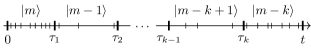
Figure 2: Parametrization of a quantum trajectory build from two types of quantum jumps $L_{a}=\sqrt{\kappa_{a}}\,a$ and $L_{n}=\sqrt{\kappa_{n}}\,a^{\dagger}a$. The times $\tau_{\sigma}$ correspond to the $L_{a}$ jumps and the quantum state between each jump is above each slice.

For a given slice $\sigma\in[\![1,k+1]\!]$ where $\tau_{k+1}=t$ and $\tau_{0}=0$, the relative state obtained from Eq. 10 is proportional to the Fock state $\ket{m-\sigma}$. By denoting $\alpha(t,[\mu])$ the proportionality constant, we find:

$$\ket{\psi_{c}(\tau_{\sigma},[\mu])}=\prod_{s=1}^{N_{\sigma-1}}\left(-\mathrm{i}\sqrt{\kappa_{n}\mathrm{d}t_{\sigma-1,s}}(m-\sigma+1)\right)$$

$$\times\left(-\mathrm{i}\sqrt{\kappa_{a}\mathrm{d}\tau_{\sigma}(m-\sigma+1)}\right)$$

$$\times\mathrm{e}^{-\left(\mathrm{i}(m-\sigma+1)\omega_{c}+(m-\sigma+1)^{2}\kappa_{n}/2+(m-\sigma+1)\kappa_{a}/2\right)(\tau_{\sigma}-\tau_{\sigma-1})}$$

$$\times\alpha(\tau_{\sigma-1},[\mu])\ket{m-\sigma}\,.$$ (11)

Having the formal form of the state of the system relative to a given quantum trajectory, we can obtain the reduced density matrix by summing over all possible trajectories. Our parametrization is such that we can re-sum all the phases accumulated between each $L_{a}$ jumps easily and then average over all $L_{a}$ jump events. For the initial Fock state $\ket{m}$, only the diagonal elements of the reduced density matrix can be non zero. No coherences are induced since a Fock state remains a Fock state and no superposition appears. This immensely simplifying feature comes directly from the special commutation relation of the jump operators. We obtain:

$$\rho_{m-k,m-k}={m\choose k}(1-\mathrm{e}^{-\kappa_{a}t})^{k}\mathrm{e}^{-\kappa_{a}t(m-k)}\,.$$ (12)

Starting from a Fock state $\ket{m}$, the state $\ket{m-k}$ is reached if $k$ photons have leaked. The associated probability is given by $p(t,k)={m\choose k}(1-\mathrm{e}^{-\kappa_{a}t})^{k}\mathrm{e}^{-\kappa_{a}t(m-k)}$, which is the classical probability for a binomial experience $B(m,p)$, where the probability $p$ for a photon to leak between $0$ and $t$ is $p=1-\mathrm{e}^{-\kappa_{a}t}$. We recover the standard evolution of a damped harmonic oscillator prepared in a Fock state.

The coupling constant $\kappa_{n}$ does not appear in this expression which means that the dephasing induced by an atom flux has no effect on a Fock state. Indeed, we saw that $L_{n}$ jumps induce a dephasing between Fock states. Since a unique trajectory keeps the cavity in a single Fock state, this dephasing is only a global phase shift and thus has no effect at all.

Since Fock states form a basis of the Hilbert space of the system, an analogous computation starting from any superposition of Fock states gives the general solution:

$$\rho_{m,n}(t) =\mathrm{e}^{-\mathrm{i}\omega(m-n)t}\mathrm{e}^{-\kappa_{a}\frac{m+n}{2}t}\mathrm{e}^{-\frac{\kappa_{n}}{2}(m-n)^{2}t}$$

$$\times\sum_{N_{a}}\sqrt{{m+N_{a}\choose N_{a}}{n+N_{a}\choose N_{a}}}(1-\mathrm{e}^{-\kappa_{a}t})^{N_{a}}$$

$$\times\rho_{m+N_{a},n+N_{a}}(0)\,.$$ (13)

The physical content of this general exact expression is more transparent if we initially prepare a superposition of coherent states. What’s more, those are the typical quantum states that are used in cavity quantum electrodynamics to study the decoherence process. Let’s then consider the state $\ket{\Psi_{c}}=\frac{\ket{\alpha_{+}}+\ket{\alpha_{-}}}{\sqrt{\mathcal{N}}}$ where $\alpha_{\pm}=\alpha\,\mathrm{e}^{\pm\mathrm{i}\theta/2}$, $\alpha\in\mathbb{C}$ and $\mathcal{N}$ is a normalization factor. The initial density matrix is then given by:

$$\rho_{m,n}(0) =\frac{1}{\mathcal{N}}\big{(}\rho_{m,n}(\alpha_{+})+\rho_{m,n}(\alpha_{-})$$

$$+\rho_{m,n}(\alpha_{+},\alpha_{-})+\rho_{m,n}(\alpha_{-},\alpha_{+})\big{)}\,,$$ (14)

where $\rho_{m,n}(\alpha)=\langle m|\alpha\rangle\langle\alpha|n\rangle$ refers to the matrix element $mn$ in the Fock basis of the density matrix of the coherent state $\ket{\alpha}$. The last two terms correspond to interferences between the two coherent states, with $\rho_{m,n}(\alpha_{+},\alpha_{-})=\langle m|\alpha_{+}\rangle\langle\alpha_{-}|n\rangle$. Using Eq. 13, the time-evolved density matrix at time $t$ is given by:

$$\rho_{m,n}(t)=\frac{1}{\mathcal{N}}\mathrm{e}^{-\kappa_{n}\frac{(m-n)^{2}}{2}t}\big{[}\rho_{m,n}(\alpha_{+}(t))+\rho_{m,n}(\alpha_{-}(t))\\ +\mathrm{e}^{-|\alpha|^{2}(1-\mathrm{e}^{-\kappa_{a}t})(1-\mathrm{e}^{\mathrm{i}\theta})}\rho_{m,n}(\alpha_{+}(t),\alpha_{-}(t))+\text{h.c.}\big{]}\,,$$ (15)

where $\alpha_{\pm}(t)=\alpha_{\pm}\,\mathrm{e}^{-\mathrm{i}\omega_{c}t}\mathrm{e}^{-\frac{\kappa_{a}}{2}t}$. The effect of the two decoherence channels can be clearly identified. First, the term $d_{a}(t)=\mathrm{e}^{-|\alpha|^{2}(1-\mathrm{e}^{-\kappa_{a}t})(1-\mathrm{e}^{\mathrm{i}\theta})}$ is the usual decoherence factor coming from the jump $L_{a}=\sqrt{\kappa_{a}}a$ (damped harmonic oscillator) which tends to destroy coherences between coherent states. On the other hand, the term $\mathrm{e}^{-\kappa_{n}\frac{(m-n)^{2}}{2}t}$ tends to destroy coherences between Fock states which are the natural pointer states of the channel $L_{n}=\sqrt{\kappa_{n}}N$.

The interesting and surprising aspect of Eq. 15 is that, while the Lindblad jump operators do not commute, the overall evolution is, in a sense, decoupled. This can be made precise by using the quantum channels perspective. Indeed, by considering the superoperators $\boldsymbol{H}=-\mathrm{i}(\bar{H}\otimes\mathbbm{1}-\mathbbm{1}\otimes H)$ and $\boldsymbol{D}=\sum_{\mu}\bar{L}_{\mu}\otimes L_{\mu}-\frac{1}{2}\mathbbm{1}\otimes L_{\mu}^{\dagger}L_{\mu}-\frac{1}{2}\bar{L}_{\mu}^{\dagger}\bar{L}_{\mu}\otimes\mathbbm{1}$ (the bar notation corresponds to complex conjugation), the Lindbald equation can be formally integrated as Havel (2003):

$$\rho(t)=\mathrm{e}^{(\boldsymbol{H}+\boldsymbol{D})t}\rho(0)=\mathcal{L}_{H,[L_{\mu}]}(t)\rho(0)\,.$$ (16)

The notation $\mathcal{L}_{H,[L_{\mu}]}(t)$ is here to remind us that the quantum channel depends on the set of jump operators $L_{\mu}$ through the operator $\mathcal{D}$. In our problem, we have two non-commuting jump operators $L_{a}=\sqrt{\kappa_{a}}\,a$ and $L_{n}=\sqrt{\kappa_{n}}N$. Astonishingly, their respective quantum channels do commute, leading to:

$$\mathcal{L}_{H,L_{a},L_{N}}(t)=\mathcal{L}_{H,L_{a}}(t)\mathcal{L}_{L_{N}}(t)=\mathcal{L}_{L_{N}}(t)\mathcal{L}_{H,L_{a}}(t)\,.$$ (17)

Thus, while the generators of the open quantum dynamics do not commute, the associated quantum channels do (and decouple in this sense). The full dynamics of the model can be solved by parts by looking at the evolution of both quantum channels separately, which is an easy task. Nevertheless, this does not trivialize the einselection problem of finding the exact or approximate pointer states that entangle the least with the environment. The emergence of a classical picture does depend on the “fine structure” of the dynamics.

Table 1: Comparison of the timescales relative to the classes of exact pointer states

Timescale	Expression	Coherent state (C)	Fock state (F)
Decoherence of coherence states	$\tau_{a}=1/2\,\langle n\rangle\kappa_{a}\sin^{2}(\theta/2)$	Decoherence (C)	Spreading
Relaxation	$\tau_{r}=1/\kappa_{a}$	Relaxation	Relaxation & Decoherence (C)
Spreading in angle	$\tau_{s}=2/\kappa_{n}\langle n\rangle$	Spreading	Decoherence (F)
Crown formation	$\tau_{c}=1/\kappa_{n}$	Decoherence (F)	✗

Two natural decoherence timescales can be defined, still considering the initial state to be the superposition of coherent states $\ket{\Psi_{c}}$. The first one is the usual decoherence timescale $\tau_{a}$ of a superposition of coherent states induced by the decoherence channel $L_{a}$. Its expression is directly given by the exponential modulation of the coherence term in the general solution Eq. 15:

$$\tau_{a}=\frac{1}{2\,\langle n\rangle\,\kappa_{a}\,\sin^{2}(\theta/2)}\,,$$ (18)

using that $|\alpha|^{2}=\langle n\rangle$. Over time, this channel tends to empty the cavity. The relaxation timescale $\tau_{r}$ deduced from the equation $\alpha(t)=\mathrm{e}^{-\kappa_{a}t/2}\alpha$ is such that:

$$\tau_{r}=\frac{1}{\kappa_{a}}\,.$$ (19)

A second decoherence timescale $\tau_{n}$ is associated to the $L_{n}$ channel. In the Fock basis, its expression is straightforwardly given by $\tau_{s}=2/\kappa_{n}(m-n)^{2}$. Still, we can rewrite it in a form more suitable for coherent states. Indeed, coherent states have a Poissonian distribution of photons with an average $\langle n\rangle=|\alpha|^{2}$ and a variance $\Delta n=\sqrt{|\alpha|^{2}}=\sqrt{\langle n\rangle}$. Thus, the characteristic width $\Delta n$ of a coherent state gives a characteristic upper bound $m-n\leq\Delta n$. This allows us to extract a characteristic time which, as we will see, correspond to a spreading in the angle variable in phase space:

$$\tau_{s}=\frac{2}{\kappa_{n}\langle n\rangle}\,.$$ (20)

This timescale corresponds to the short time effect of $L_{n}$. The long time effect is given for $m-n=1$ and corresponds to a disappearance of the Fock states superposition. The associated timescale $\tau_{c}$, which corresponds to the formation of a rotation-invariant crown in phase space, is given from Eq. 15 by:

$$\tau_{c}=\frac{1}{\kappa_{n}}\,.$$ (21)

Thus, the two natural decoherence timescales for coherent states are $\tau_{a}$ and $\tau_{c}$, corresponding to the loss of coherence on the coherent state and number state basis respectively. The scaling $\tau_{a}/\tau_{c}\simeq\kappa_{n}/\kappa_{a}\langle n\rangle$ implies that for sufficiently high energy, we can have a separation of decoherence times, by first seeing a decoherence over the coherent states followed by one on the number basis. Table 1 summarizes the different timescales, their expression and interpretation when a superposition of coherent states is initially prepared. However, as we will see over the next sections, the interpretation of those timescales is relative to the class of pointer states we use like, for instance, when we initially prepare Fock states.

III.3 Phase-space approach

III.3.1 The general solution

Last section presented the general solution of the Lindblad Eq. 4 using the quantum trajectories approach. It is also possible to solve the same problem from a phase-space perspective using characteristic functions of the density matrix. This approach offers interesting physical insights on the dynamical evolution imposed by the two incompatible channels.

Given a density operator $\rho$, we associate a function $C_{\rho}(\lambda,\lambda^{*})$, with $\lambda\in\mathbb{C}$, defined as:

$$C_{\rho}(\lambda,\lambda^{*})=\operatorname{tr}\left(\rho\mathrm{e}^{\lambda b^{\dagger}}\mathrm{e}^{-\lambda^{*}b}\right)\,.$$ (22)

This function is called the characteristic function adapted to the normal order. All the normally-ordered average values can be recovered from it. It is an integral transform of the Wigner function that we will define and use extensively latter on. Now, by taking each term of the Lindblad Eq. 4, it is a straightforward computation, using the BCH formula, to write it in terms of the characteristic function as:

$$\partial_{t}C_{\rho}+\lambda\left(\frac{\kappa_{a}}{2}-\mathrm{i}\omega_{c}\right)\,\partial_{\lambda}C_{\rho}+\lambda^{*}\left(\frac{\kappa_{a}}{2}+\mathrm{i}\omega_{c}\right)\,\partial_{\lambda^{*}}C_{\rho}\\ =-\frac{\kappa_{n}}{2}(\lambda\partial_{\lambda}-\lambda^{*}\partial_{\lambda^{*}})^{2}\,C_{\rho}\,.$$ (23)

By using polar coordinates $\lambda=r\,\mathrm{e}^{\mathrm{i}\theta}$, we obtain the more transparent form:

$$\left(\partial_{t}+\frac{\kappa_{a}}{2}r\partial_{r}-\omega_{c}\partial_{\theta}\right)C_{\rho}(r,\theta,t)=\frac{\kappa_{n}}{2}\partial^{2}_{\theta}C_{\rho}(r,\theta,t)\,.$$ (24)

This equation is of the Fokker-Planck type with the right-hand side being a diffusion term with a diffusion coefficient given by the coupling constant $\kappa_{n}$. Thus, the channel $L_{n}$ tends to spread in angle the characteristic function. This is in accord with the first discussion of the evolution of fluctuations given through the average values. Note that we could even consider an environment at finite temperature and obtain a similar equation (with an inhomogeneous term) that can also be solved exactly.

When only the channel $L_{a}$ is present, the differential equation is first order and can be solved by the method of characteristics Carmichael (1999); Arnol’d (2013). This is not directly the case here but can be remedied by going to the Fourier domain with respect to the variable $\theta$. Doing this is indeed quite intuitive if we remember that the conjugated observable associated to $\theta$ is the number operator $N$ which is the natural observable of the problem, and that both are related by a Fourier transform.

Let’s then define a new characteristic function $C_{\rho}(r,n)=\int C_{\rho}(r,\theta)\,\mathrm{e}^{\mathrm{i}n\theta}\,\mathrm{d}\theta$ which is the Fourier series of $C_{\rho}(r,\theta)$. We then end up with an in-homogeneous first-order partial differential equation:

$$\left(\partial_{t}+\frac{\kappa_{a}}{2}r\partial_{r}\right)C_{\rho}(r,n,t)=\left(\mathrm{i}\omega_{c}n-n^{2}\right)\frac{\kappa_{n}}{2}C_{\rho}(r,n,t)\,.$$ (25)

By applying the method of characteristics, solving the equations $\dot{r}=\kappa_{a}$ and $\dot{n}=0$, we obtain the general solution for an initial condition $C_{0}(r_{0},n_{0})$:

$$C_{\rho}(r,n,t)=C_{0}(r\mathrm{e}^{-\kappa_{a}t/2},n)\,\mathrm{e}^{\left(\mathrm{i}\omega_{c}n-\frac{\kappa_{n}}{2}n^{2}\right)t}\,.$$ (26)

From the radial damping, we recover the usual damping rate leading to decoherence on the coherent state basis. Besides this usual behavior, we have a new damping term depending on the square of the Fock variable $n$ which leads to the decoherence in the Fock basis with the characteristic angle-spreading timescale $\tau_{s}$ already uncovered in Section III.2.

III.3.2 Fock state decoherence

Different initial states can be prepared. We will naturally focus on two classes of states, Fock states $\ket{n}$ and coherent states $\ket{\alpha}$. As a warm up example, suppose that only the channel $L_{n}$ is present. If we prepare a Fock state $\ket{n}$, whose characteristic function is given by $C_{\ket{n}}(\lambda)=\mathcal{L}_{n}(|\lambda|^{2})$ where $\mathcal{L}_{n}$ is the Laguerre polynomial of order $n$, we know that it will not be affected by the environment and will evolve freely as can be readily checked from Eq. 26. The important remark here is that the phase-space representation of a Fock state or any statistical mixture of them is rotation invariant.

If we now prepare a quantum superposition of Fock states $(\ket{n_{0}}+\ket{n_{1}})/\sqrt{2}$, it is straighforward to show that the coherence part of the characteristic function ${C_{01}(\lambda,\lambda^{*})=\operatorname{tr}\left(\ket{n_{0}}\!\!\bra{n_{1}}\mathrm{e}^{\lambda b^{\dagger}}\mathrm{e}^{-\lambda^{*}b}\right)}$ evolves as:

$$C_{01}(\lambda,\lambda^{*})=\mathrm{e}^{-\frac{\kappa_{n}}{2}(n_{1}-n_{0})^{2}t}C_{01}(r,(\omega_{c}-\theta)t)\,.$$

The coherence term between Fock states are damped by an exponential factor with a characteristic timescale $2/(n_{0}-n_{1})^{2}\kappa_{n}$ scaling as the quadratic inverse of the “distance” between the two components of the state. The is the expected decoherence dynamics for the exact pointer states of a decoherence channel.

III.3.3 Coherent states and the Wigner representation

In the spirit of cavity quantum electrodynamics experiments, it is more appropriate to study the evolution of coherent states and their superposition. Before discussing the dynamics of such states, it is necessary to introduce a better-suited phase-space representation then the one defined by Eq. 22. Indeed, this latter function is a complex-valued function which is not the best choice for representation purposes. From the characteristic function $C_{\rho}(\lambda,\lambda^{*})$, we can recover an equivalent, real-valued, phase-space representation called the Wigner function $W_{\rho}(\alpha)$ of the state $\rho$ (with the parameter $\alpha\in\mathbb{C}$) defined as the following integral transform Wigner (1932); Carmichael (1999):

$$W_{\rho}(\alpha)=\frac{1}{\pi^{2}}\int C_{\rho}(\lambda)\,\mathrm{e}^{-|\lambda|^{2}/2}\,\mathrm{e}^{\alpha\lambda^{*}-\alpha^{*}\lambda}\,\mathrm{d}^{2}\lambda\,.$$ (27)

Using the position and momentum coordinates in phase space $\alpha=x+\mathrm{i}p$, we recover the common expression:

$$W_{\rho}(x,p)=\int\langle x+u/2|\rho|x-u/2\rangle\,\mathrm{e}^{-\mathrm{i}up}\,\frac{\mathrm{d}u}{2\pi}\,,$$ (28)

where the states $\ket{x}$ are eigenstates of the position operator $x\propto a+a^{\dagger}$. The Wigner function is used in a wider context than quantum optics Ville (1948); Flandrin (1998) and possesses a nice set of properties to represent quantum interferences in a transparent way. We will use it throughout this paper to represent our analytical and numerical results. Furthermore, since the proper dynamics of the field mode can be factored out, the dynamics is pictured without the rotation in phase space that it introduces.

Both for the numerical calculations as well as for understanding the dynamics in phase space, it is helpful to write the Wigner function in terms of its Fourier components of the polar angle $\theta$. Thus, let’s decompose the Wigner function on the Fock state basis as:

$$W(x,p) =\sum_{m,n}\rho_{mn}W_{mn}\,,$$ (29)

$$W_{mn}(x,p) =\int\Braket{x+\chi/2}{m}\Braket{n}{x-\chi/2}\mathrm{e}^{-\mathrm{i}p\chi}\,\frac{\mathrm{d}\chi}{2\pi}\,.$$ (30)

If we denote $x+\mathrm{i}p=r\mathrm{e}^{\mathrm{i}\theta}$, we find that for $l\geq 0$:

$$W_{k,k+l}(r,\theta)=\frac{(-1)^{k}}{\pi}\sqrt{2^{l}\frac{k!}{(k+l)!}}\mathrm{e}^{-\mathrm{i}l\theta}r^{k}L_{k}^{l}(2r^{2})\,,$$ (31)

where $L_{m}^{k}$ are generalized Laguerre polynomials. This implies that the coherence given by $\rho_{k,k+l}$ ($k\in\mathbb{N},l\geq 0$) and $\rho_{k-l,k}$ ($k\in\mathbb{N},l\leq 0$) corresponds to the $l$th harmonics of the angle variable in the Wigner function.

Notably, since the $L_{n}$ channel acts by multiplying all the elements situated at a distance $l$ from the diagonal by the same quantity, it corresponds to reduce the different harmonics of the angle variable by an exponential amount. This corresponds of the idea of a spread in the angle variable.

If we now prepare a coherent state $\ket{\alpha}$ whose characteristic function is given by $C_{\ket{\alpha}}(\lambda)=\mathrm{e}^{\alpha^{*}\lambda-\alpha\lambda^{*}}$, its evolution in the presence of only the $L_{n}$ decoherence channel is given by the convolution of the initial characteristic function with a Gaussian function $\mathcal{N}_{\sigma}(\theta)=\mathrm{e}^{-\theta^{2}/2\sigma^{2}}/\sqrt{2\pi\sigma^{2}}$ of the angle variable $\theta$ spreading in time with a variance $\sigma^{2}=\kappa_{n}t$ (see Section A.1). In terms of the Wigner function, we have:

$$W(r,\theta,t)=\int_{-\infty}^{+\infty}W_{0}(r,\theta^{\prime})\,\mathcal{N}_{\sigma^{2}=\kappa_{n}t}\left(\theta-\theta^{\prime}\right)\,\mathrm{d}\theta^{\prime}\,.$$ (32)

with $W_{0}$ the initial Wigner function. This form displays clearly the diffusive dynamics induced by the $L_{n}$ decoherence channel in the phase angle, putting the initial intuition on firm ground.

Figure 3 represents the evolution of the Wigner function of a superposition of coherent states. At a time scale $\tau_{s}=2/\kappa_{n}\langle n\rangle$, the Gaussian spots start to spread along circles with a radius given by their respective amplitude. The same can be said for the Gaussian interference spot which is centered at the mid-point in phase space. At later times $t\gtrsim\tau_{c}$, the coherent states spread uniformly and are completely decohered as a statistical mixture of Fock states.

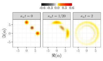
Figure 3: Evolution of a superposition of coherent states from $t=0$, subject to the $L_{n}$ channel only ($\kappa_{a}=0$) in the Wigner function representation. The Gaussian spots are spread over a timescale given by $\kappa_{n}\tau_{s}=2/\langle n\rangle$. For the chosen parameters $\alpha=\sqrt{40}$, it is given by $\kappa_{n}\tau_{s}=1/20$. At longer times $\kappa_{n}t=2$, the superposition evolves toward a statistical mixture of Fock states with the characteristic rotation invariance in phase space.

In fact, we can better understand the structure of the Wigner function at finite times by explicitly writing the periodicity in the variable $\theta$ hidden in Eq. 32. Indeed, we have $W(r,\theta,t)=\int_{0}^{2\pi}W_{0}(r,\theta^{\prime})\,\vartheta\left(\frac{\theta-\theta^{\prime}}{2\pi};\mathrm{i}\frac{\kappa_{n}t}{2\pi}\right)\,\frac{\mathrm{d}\theta^{\prime}}{2\pi}$ with $\vartheta(z;\tau)=\sum_{n\in\mathbb{Z}}\exp(\pi\mathrm{i}n^{2}\tau+2\pi\mathrm{i}nz)$ the Jacobi theta function. When $\kappa_{n}t\gg 1$, the expansion $\vartheta\left(\frac{\theta}{2\pi};\mathrm{i}\frac{\kappa_{n}t}{2\pi}\right)\simeq 1+2\sum_{n\in\mathbb{N}^{*}}\left(\mathrm{e}^{-\kappa_{n}t/2}\right)^{n^{2}}\cos n\theta$ can be used to approximate the Wigner function. For instance, if $\kappa_{n}t=2$, only the first harmonic of the Wigner function dominates with oscillations in amplitude of $74\text{\,}\mathrm{\char 37\relax}$ of the average value, the second harmonic being less than $2\text{\,}\mathrm{\char 37\relax}$, as can be seen on Figs. 3 and 4. This harmonic decomposition also shows that in the presence of symmetries in angle, for instance $W(r,\theta+2\pi/p)=W(r,\theta)$ for an integer $p\geq 2$, the first non-zero modulation term scales as $\mathrm{e}^{-\kappa_{n}tp^{2}/2}$. Thus, symmetric initial states will decohere much quicker than the ones that are not.

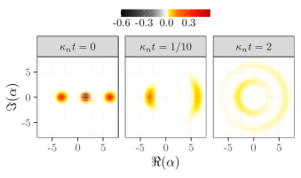
Figure 4: Depending on the preparation, with for instance here $\alpha_{+}=\sqrt{40}$ and $\alpha_{-}=-\sqrt{10}$, the interference spot is totally washed out by the $L_{n}$ channel ($\kappa_{a}=0$) after the spreading timescale $\kappa_{n}t=1/10$ leading at longer times $\kappa_{n}t=2$ to a mixture of Fock states.

Finally, note that the presence of an interference pattern on Fig. 3 is not a signature of coherence between Fock state. For a different preparation like the one on Fig. 4, the interference spot is completely washed out over a timescale of $\tau_{s}$.

IV Einselection process

Now that we have a proper analytic solution of the problem and that we completely understand the evolution and characteristic timescales of each decoherence channel separately, which is summarized in Fig. 5, we can analyze the einselection process in its full generality.

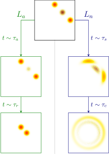
Figure 5: Summary of different evolution and timescales of a superposition of coherent states under the effects of two decoherence channels: the $L_{n}$ channel induces a spreading of the wavepacket while the $L_{a}$ channel destroys interferences and makes the system relaxes to the vacuum.

IV.1 Pointer states dynamics

Intuitively, we expect the classical picture that emerges must be dominated by the quantum channel which has the strongest coupling constant Novais et al. (2005). We can in fact play with two parameters, the ratio $\kappa_{n}/\kappa_{a}$ and the average energy of the state $\langle n\rangle$.

One regime is when we have $\tau_{a}/\tau_{c}\approx\kappa_{n}/\kappa_{a}\langle n\rangle\gg 1$ or equally $\langle n\rangle\ll\kappa_{n}/\kappa_{a}$. We expect in this case that Fock state decoherence dominates the dynamics. We can refine our statement by unraveling two subregimes with respect to the relaxation timescale $\tau_{r}$:

• In the range $\tau_{c}\ll\tau_{a},\tau_{r}$, or equally $\langle n\rangle\ll\kappa_{n}/\kappa_{a}$ and $\tau_{r}/\tau_{c}\approx\kappa_{n}/\kappa_{a}\gg 1$, we have a proper decoherence on the Fock basis as we expected.

• However, for $\tau_{r}\ll\tau_{c}\ll\tau_{a}$, or equally $\langle n\rangle\ll\kappa_{n}/\kappa_{a}$ and $\tau_{r}/\tau_{c}\approx\kappa_{n}/\kappa_{a}\ll 1$, we end up in the almost degenerate case $\langle n\rangle\ll 1$ where we relax on the vacuum state.

Thus, in the regime $\tau_{a}\gg\tau_{c}$ where the Fock decoherence dominates initially, we see that the relaxation induced by the $L_{a}$ channel forbids to transition toward a proper non-trivial coherent-state classical picture: before evolving towards a proper statistical mixture of coherent states, the system relaxes to the vacuum. All in all, the emergent physically meaningful classical picture is given by Fock states.

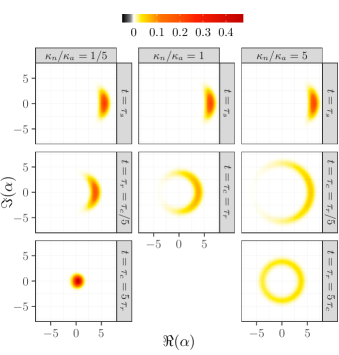
Figure 6: Coherent state dynamics for $\alpha=\sqrt{40}\gg\kappa_{n}/\kappa_{a}$. Depending on the relative ratio of the coupling constants $\kappa_{n}/\kappa_{a}$ we either see a emergent classical picture based solely on coherent states $\kappa_{n}/\kappa_{a}<1$ or both coherent and then Fock states ($\kappa_{n}/\kappa_{a}>1$).

From the einselection perspective, a richer dynamics can be found in the complementary regime where $\tau_{a}/\tau_{c}\approx\kappa_{n}/\kappa_{a}\langle n\rangle\ll 1$ or equally $\langle n\rangle\gg\kappa_{n}/\kappa_{a}$. Figure 6 shows the evolution of the Wigner function of a coherent state (with initially 40 photons on average) for this situation. We can at least see three different regimes:

• The regime with $\kappa_{a}\gg\kappa_{n}$ (first column with $\kappa_{a}=5\,\kappa_{n}$). In this case, we see that coherent states remain largely unaffected by the environment and evolves according to the dynamics of the $L_{a}$ channel with the characteristic dissipation timescale $\tau_{r}$.

• The complementary regime with $\kappa_{n}\gg\kappa_{a}$ (third column with $\kappa_{n}=5\,\kappa_{a}$) where the $L_{n}$ rules the dynamical evolution. We see that the coherent state is spread into a statistical mixture of Fock states over a timescale $\tau_{c}$ which is then followed by the much slower process of relaxation.

• The intermediate regime with $\kappa_{a}\approx\kappa_{n}$. In this case, it is not possible to clearly conclude which basis is the most classical one.

The previous discussion focused mainly on a preparation of coherent states. A similar discussion can be made if we prepare a Fock state. As expected, if the $L_{n}$ channel dominates, we observe a decoherence over the Fock basis with a slow relaxation towards the vacuum induce by the $L_{a}$ channel. Nonetheless, some subtleties, detailed in Section A.2, occur in the opposite situation because coherent states do not form a proper orthogonal basis. In the same way that a very close superposition of coherent states will not properly decohere under the influence of the $L_{a}$ channel, a Fock state, being a continuous superposition of coherent states, cannot properly evolve toward a classical mixture of coherent states.

IV.2 Approximate pointer states

For a general dynamics, exact pointer states, defined as states that do not get entangled with the environment if they are initially prepared, do not exist. Instead, we have to rely on an approximate notion of pointer states to give a meaningful notion of an emergent classical description. Approximate pointer states are defined as the states that entangle the least with the environment according to a given entanglement measure. This definition of approximate pointer states, called the predictability sieve and used in different contexts Kiefer et al. (2007); Riedel (2016), is one definition among different proposal to formalize the idea of robustness against the environment. For instance, the Hilbert-Schmidt robustness criterion Gisin and Rigo (1995); Busse and Hornberger (2009) defines pointer states to be time-dependent pure states that best approximate according to the Hilbert-Schmidt norm the impure state generated by infinitesimal time evaluation. Fortunately, those different approaches were shown to be consistent for physically meaningful models Diósi and Kiefer (2000).

Many different measures of entanglement exist in quantum information theory and it is not yet totally clear which one is the proper one to use in the predictability sieve approach. For the sake of simplicity, we will consider the purity $\gamma$ defined as :

$$\gamma=\operatorname{tr}\rho^{2}\,.$$ (33)

Approximate pointer states are then defined by searching for pure states that minimize the initial variation of the entropy or, in our case, maximize the variation of purity. It’s worth noting that the purity variation, for a pure state, is also equal to twice the variation of the principal eigenvalue of the density matrix.

Before proceeding, we could inquire about the dependence of the approximate pointer states that we find on the entanglement witness that we choose. For instance, we could have chosen a whole class of entropies $S_{\alpha}$ called the Rényi entropies Rényi et al. (1961) defined as $S_{\alpha}(\rho)=\frac{1}{1-\alpha}\operatorname{tr}\rho^{\alpha}$. Using those entropies to find approximate pointer state do not change the conclusion if we are looking at the short-time evolution of a pure state. Indeed, if we prepare at $t=0$ a pure state, we have that $\rho^{\alpha}=\rho$ for $\alpha\neq 0$. Then $\dot{S}_{\alpha}=\frac{\alpha}{1-\alpha}\operatorname{tr}\dot{\rho}\rho^{\alpha-1}=\frac{\alpha}{1-\alpha}\operatorname{tr}\dot{\rho}\rho$ which is equal, apart from a proportionality factor, to the evolution of purity. The approximate pointer states do not then depend on which measure we choose.

Coming back to the purity, its derivative $\dot{\gamma}$, which is, up to a constant factor, just the derivative of the largest eingenvalue for an initial pure state, is linear in $\partial_{t}\rho$. We thus have $\dot{\gamma}=\dot{\gamma}_{a}+\dot{\gamma}_{n}$, where $\dot{\gamma}_{a}$ (resp. $\dot{\gamma}_{n}$) is the contribution solely due to the $L_{a}$ (resp. $L_{n}$) channel. First of all, since each of these contributions is non positive, a pure state will stay pure if and only if it stays pure for each channel. In this case, it is easy to see that, unless one of the two constants $\kappa_{a}$ or $\kappa_{n}$ is zero, the only state staying pure is the vacuum state. That’s why, in general, no exact pointer states exist for a complex open quantum dynamics and we have to look for approximate ones. Having said that, we now have to search for pure states that maximize the evolution of the purity at initial time. As a function of the matrix elements $\rho_{mn}$ of the initial state written in the Fock basis, the purities satisfy the equations:

$$\dot{\gamma}_{n} =-\kappa_{n}\sum_{m,n}|\rho_{m,n}|^{2}(m-n)^{2}\,,$$ (34a)

$$\dot{\gamma}_{a} =-\kappa_{a}\sum_{m,n}\Big{[}|\rho_{m,n}|^{2}(m+n)$$

$$-2\rho_{m,n}^{*}\rho_{m+1,n+1}\sqrt{(m+1)(n+1)}\Big{]}\,.$$ (34b)

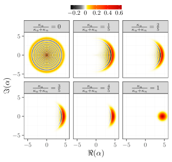
Figure 7: Wavepacket that minimizes the loss of purity at initial time, for an average energy of $20$ photons, obtained by numerical optimization techniques. The optimal (with respect to the purity) state $\dot{\gamma}_{\text{opt}}$ interpolates between Fock states and coherent states depending on the relative value $\kappa_{a}/(\kappa_{a}+\kappa_{n})$ of the coupling constants.

To find the approximate pointer states, we thus have to optimize the initial pure state that minimize the absolute purity variation, under the constraint of a unit norm. It is also natural to fix the average energy of the wavepacket (otherwise, the vacuum is a trivial optimum). Since it is difficult to perform this optimization analytically, we performed it numerically using the Pagmo library Biscani et al. (2019) with the SNOPT algorithm Gill et al. (2005). We see on Fig. 7 that, when the average energy is a multiple of the number of photons, the optimal state deforms from a coherent state to a Fock state. The optimal purity variation, $\dot{\gamma}_{\text{opt}}$ as a function of $(\kappa_{a},\kappa_{n})$, can be seen for different number of photons on Fig. 9.

The time evolution of the approximate pointer states is featured on Fig. 8. This illustrates that on short timescales, the optimal state keeps its shape and, as such, is quite robust to both interactions.

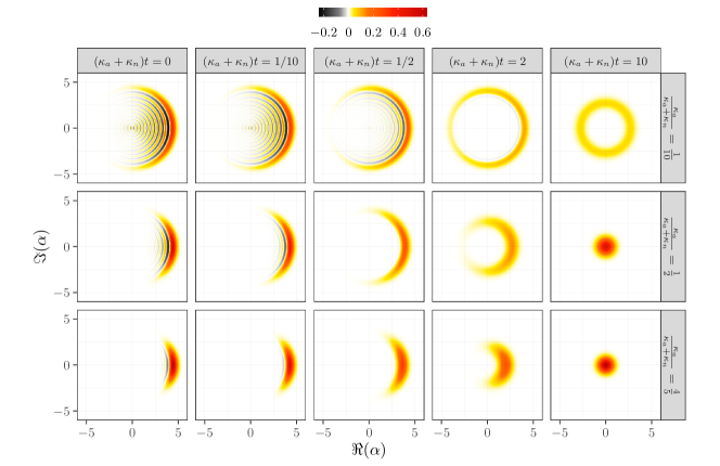
Figure 8: Evolution of the approximate pointer states for several $(\kappa_{a},\kappa_{n})$ parameter regimes, for an initial energy of $n_{0}=20$ photons.

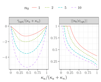
Figure 9: Purity and scalar product of the approximate pointer state with Fock states for energies of $n_{0}=1,2,5,10$ photons. We see that in the low $\kappa_{a}$ regime, the approximate pointer state $\ket{\psi_{\text{opt}}}$ is still a Fock state, until the critical value $\kappa_{n}/\kappa_{a}=n_{0}+\sqrt{n_{0}(n_{0}+1)}+1/2$. As expected, the variation of purity linearly decreases on this plateau.

Furthermore, a remarkable fact can be seen by looking at the overlap between the Fock state of energy $n_{0}$ and the optimal pure state $\ket{\psi_{\text{opt}}}$: Fock states remain the approximate pointer states even in the presence of the $L_{a}$ decoherence channel at small coupling $\kappa_{a}\ll\kappa_{n}$. This is characterized by the presence of a plateau on the overlap $|\langle n_{0}|\psi_{\text{opt}}\rangle|$ as a function of $\kappa_{a}/(\kappa_{a}+\kappa_{n})$ as shown on Fig. 9.

To better understand this phenomenon, it is instructive to look at the evolution of the purity for a state not far away from the Fock state $\ket{n_{0}}$ and see how this small perturbation changes or not the optimal problem. Assuming that the state $\ket{\psi}=\sum_{n}c_{n}\ket{n}$ has coefficients $c_{n}=\delta_{n,n_{0}}+\epsilon_{n}$, with $|\epsilon_{n}|\ll 1$, we have:

$$\dot{\gamma}_{n} =-2\,\kappa_{n}\sum_{n}|\epsilon_{n}|^{2}(n-n_{0})^{2}\,,$$ (35)

$$\dot{\gamma}_{a} =-2\,\kappa_{a}\Big{(}n_{0}(1+2\Re\epsilon_{n_{0}})^{2}+\sum_{n}|\epsilon_{n}|^{2}(n+n_{0})$$

$$-|\epsilon_{n_{0}+1}|^{2}(n_{0}+1)-|\epsilon_{n_{0}-1}|^{2}n_{0}$$

$$-2\Re\epsilon_{n_{0}+1}\epsilon_{n_{0}-1}^{*}\sqrt{n_{0}(n_{0}+1)}\Big{)}\,.$$ (36)

The norm and energy constraints can be rewritten as the equation system:

$$2\Re\epsilon_{n_{0}}+\sum_{n}|\epsilon_{n}|^{2} =0\,,$$ (37a)

$$\sum_{n}(n-n_{0})|\epsilon_{n}|^{2} =0\,.$$ (37b)

Using the global phase symmetry of the quantum state, we can fix $\epsilon_{n_{0}}$ (an imaginary part on $\epsilon_{n_{0}}$ corresponds to changing the phase of the initial Fock state). Furthermore, using both constraints, we can eliminate all the terms containing $\epsilon_{n_{0}}$. The variation of purity takes the form:

$$\frac{\dot{\gamma}}{2} =\kappa_{a}n_{0}-\sum_{n}|\epsilon_{n}|^{2}\kappa_{n}(n-n_{0})^{2}$$

$$+\kappa_{a}\Big{(}|\epsilon_{n_{0}+1}|^{2}(n_{0}+1)+|\epsilon_{n_{0}-1}|^{2}n_{0}$$

$$+2\Re\epsilon_{n_{0}+1}\epsilon_{n_{0}-1}^{*}\sqrt{n_{0}(n_{0}+1)}\Big{)}\,.$$ (38)

We see that under the normalization constraint, Fock states are always stationary points of the purity variation. Furthermore, provided that $\kappa_{n}>4\kappa_{a}$, the purity variation is a maximum along all directions except possibly on the plane $(\epsilon_{n_{0}-1},\epsilon_{n_{0}+1})$. We can thus concentrate on this plane. In this case, the constraint Eq. 37b is simply $|\epsilon_{n_{0}-1}|^{2}=|\epsilon_{n_{0}+1}|^{2}$. If we denote $\theta$ the phase difference between $\epsilon_{n_{0}-1}$ and $\epsilon_{n_{0}+1}$, the tipping point occurs when:

$$\kappa_{n}/\kappa_{a}=n_{0}+\frac{1}{2}+\sqrt{n_{0}(n_{0}+1)}\cos\theta\,.$$ (39)

Since $\kappa_{n}$ has to be maximum, we can keep $\theta=0$. And thus:

$$\kappa_{n}/\kappa_{a}=n_{0}+\frac{1}{2}+\sqrt{n_{0}(n_{0}+1)}\approx 2\left(n_{0}+\frac{1}{2}\right)\,.$$ (40)

This equation gives the critical point where Fock states are no longer the einselected states of our dynamics and explains the qualitative features of Fig. 9. Actually, what we just shown is that a Fock state is always a stationary point of the purity variation. Given the norm and energy constraints, it moves from an extremum to a saddle point exactly when $\kappa_{n}/\kappa_{a}=n_{0}+\sqrt{n_{0}(n_{0}+1)}+1/2$, with $n_{0}$ the average energy of the state. When $n_{0}\gg 1$, $\kappa_{n}/\kappa_{a}\approx 2n_{0}+1$. As such, when $n_{0}$ becomes bigger, the size of the plateau on which the Fock state remains the einselected state becomes smaller. Away from the critical point, the most robust state becomes the state that interpolate between a number and coherent state of Fig. 7.

However, when the average number of photon $\bar{n}_{0}$ in the cavity is not an integer, the behavior is quite different. First, even when $\kappa_{a}=0$, there is no exact pointer state satisfying this constraint. The approximate pointer states in this case are superpositions of Fock states $\ket{\psi_{\text{sf}}}=\alpha\ket{\lfloor n_{0}\rfloor}+\beta\ket{\lceil n_{0}\rceil}$ with $(\alpha,\beta)$ such that the energy constraint is satisfied. Another difference is that in this case, the optimal state deforms smoothly from the superposition $\ket{\psi_{\text{sf}}}$ to the coherent state. Contrarily to the integer case, there is no tipping point, as can be seen on Fig. 10.

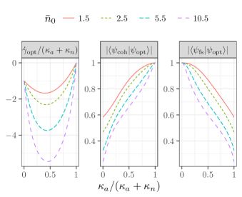
Figure 10: Purity variation, and scalar product of the approximate pointer state with the approximate pointer states when one of the coupling constant is zero. The average energy corresponds to $\bar{n}_{0}=1.5,2.5,5.5,10.5$ photons. In this case, the optimal state when $\kappa_{a}=0$ is $\ket{\psi_{\text{sf}}}=(\ket{\lfloor\bar{n}_{0}\rfloor}+\ket{\lceil\bar{n}_{0}\rceil})/\sqrt{2}$. Conversely, when $\kappa_{n}=0$, we have a coherent state whose average energy is $\bar{n}_{0}$. Contrarily to the integer case, there is no plateau appearing in the low $\kappa_{a}$ regime.

V Discussions and conclusion

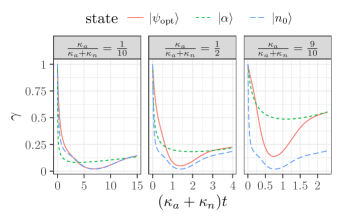
Figure 11: Evolution of the purity for the coherent state, the Fock state and the approximate pointer state for the energy $n_{0}=20$ photons.

We discussed here the einselection process in the presence of two incompatible decoherence channels and used the characterization of approximate pointer states as states that entangle the least with the environment. By choosing an entanglement measure, they are found by solving an optimization problem from the short-time open evolution of pure states (under natural constraints). Two drawbacks of this approach to the einselection problem can be stated: how the choice of the entanglement measure influences the answer and does an optimal state remain robust over time (validity of the short-time hypothesis)? As we already discussed, focusing on the short-time evolution basically solves the issue of which entanglement measure to choose, but the problem remains open in general.

From the exact solution of the model, we can compare the evolution over time of the purity between the optimal, the Fock and the coherent state of a given energy as shown in Fig. 11. As expected, we observe that, at short times, the evolution of purity is the slowest for the optimal state (by construction) while, at very long time compared to the relaxation time, everything converges toward the same value since we are basically in the vacuum. However, at intermediate timescales, the evolution of purity gets quite involved and we see that it may even be possible that the optimal state does not remain so and this is strongly dependent on the coupling constants. In this case, one can get an intuition of this behavior because the optimal states have a smaller spreading on the Fock basis than the coherent states and as such, contract to the vacuum slower. Thus, while the definition of approximate pointer states is physically intuitive, the question remains on how to properly characterize them from an information perspective but also from a dynamical perspective.

A general question that we can also ask in the perspective we adopted here on understanding the emergence of a classical picture from a complex environment would be the following: what can we learn about the dynamics and the einselection process of the model through the general features of the model like the algebraic relations between the jump operators? Naturally, the whole problem depends on the kind of dynamical approximations we do, if we start from the exact Hamiltonian dynamics or from an approximate master equation like the Lindblad equation as we did and still have in mind here.

Focusing on the general dynamics first, we saw that, given the Lindblad equation and the commutation relations of the jump operators, the dynamics can be exactly solved algebraically by adopting a quantum channel perspective: the full dynamics of the model decouples and we can look at the evolution of both quantum channels separately, which is an easy task. In fact, our solution can be abstracted in the following sense. Consider an open quantum dynamics with a damping channel encoded by the jump operator $L$ and a number decoherence channel encoded by the jump operator $L^{\dagger}L$. Our approach can then be followed steps by steps again. It however opens the question on how to defined a proper phase space associated to a jump operator (through, for instance, generalized coherent states Perelomov (2012)), how to generalize characteristic functions like the Wigner representation and verify if the phase space perspective on decoherence developed throughout our analysis still holds in this generalized context.

Concerning the einselection process however, note that having a general solution does not mean that finding the approximate pointer states is also solved. The problem remains here largely open when we have many incompatible decoherence channels. Indeed, not only does the algebraic structure influences the einselection process but also the set of coupling constants and how they run as a function of the energy Neto et al. (2003); Novais et al. (2005).

We can start to grasp those subtleties already when a thermal environment is present. Indeed, absorption processes can occur which forces us to consider a jump operator of the form $L_{a^{\dagger}}=\sqrt{\kappa_{a}\bar{n}}\,a^{\dagger}$. However, such a jump taken alone is hardly meaningful (the state evolves toward an infinite energy configuration). Relaxation processes have to be taken into account and this is summed up by the usual commutation relations between $a$ and $a^{\dagger}$. Still, this is not sufficient to reach equilibrium and proper relations between the coupling constants of the different processes must exist. This well known example already shows that relating the general features of the open quantum dynamics to the einselection process is not that straightforward.

The model studied in this paper behaves quite intuitively: when one of the coupling dominates, the associated decoherence channel controls the einselection process. However, when both couplings are comparable, the non-trivial commutation relations between the jump operators enter the game. No exact pointer basis exists and the robust states interpolate between the extreme cases and how far they are from them depends on the relative values of the coupling constants again. Still, we also unraveled the fact that, given some constraints, the transition from one class of pointer states to another as a function of the relative values of the couplings is not smooth: below a critical value, Fock states remains exactly the most robust states. How can such a behavior be anticipated from the structure of the dynamics remains to be explored. In the end, this shows that the question of predicting general features of the emergent classical picture only from the structure of the interaction (algebraic relations between jump operators, set of coupling constants) still calls for a deeper understanding.

In summary, we solved exactly a model of decoherence for an open quantum system composed of two incompatible decoherence channels using quantum trajectories and phase-space techniques. We then studied numerically the dynamical emergence of a classical picture. We were then able to see how the selection of approximate pointer states depends on the relative values of the coupling constants. This unraveled the remarkable robustness of Fock states relative to a decoherence on the coherent state basis and we were able to analyze quantitatively the critical coupling where this robustness gets lost. Our results show that the physics of decoherence and einselection still has a lot to offer when a complex dynamics is at play.

Appendix A Details on the Wigner representation

A.1 Decoherence on the Fock basis

If decoherence occurs on the Fock basis, the components are modulated by an exponential factor with a decohrence timescale inversely proportional to the “distance” between two Fock states. We can then write the Wigner function as:

$$W_{t}(r,\theta) =\sum_{l\in\mathbb{Z}}W_{l}(r)\mathrm{e}^{-\kappa_{n}l^{2}t/2}\mathrm{e}^{\mathrm{i}l\theta}$$ (41)

$$=\int_{0}^{2\pi}W_{0}(r,\theta^{\prime})\,\vartheta\left(\frac{\theta-\theta^{\prime}}{2\pi};\mathrm{i}\frac{\kappa_{n}t}{2\pi}\right)\,\frac{\mathrm{d}\theta^{\prime}}{2\pi}$$ (42)

$$=\int_{-\infty}^{+\infty}W_{0}(r,\theta^{\prime})\,\mathcal{N}_{\sigma^{2}=\kappa_{n}t}\left(\theta-\theta^{\prime}\right)\,\mathrm{d}\theta^{\prime}\,,$$ (43)

where $W_{l}(r)$ is the $l$th harmonics of the angle variable of the Wigner function at time $t=0$, $\vartheta(z;\tau)=\sum_{n\in\mathbb{Z}}\exp(\pi\mathrm{i}n^{2}\tau+2\pi\mathrm{i}nz)$ is the Jacobi theta function and $\mathcal{N}_{\sigma^{2}}$ is the centered normal distribution of variance $\sigma^{2}$.

In phase space, the dynamics induced by the $L_{n}$ channel is thus the expected Gaussian spreading of a diffusive evolution. When $\kappa_{n}t\ll 1$, the periodicity can be forgotten. However, when $\kappa_{n}t\gg 1$, we have the interesting expansion of the Jacobi function:

$$\vartheta\left(\frac{\theta}{2\pi};\mathrm{i}\frac{\kappa_{n}t}{2\pi}\right)=1+2\sum_{n\in\mathbb{N}^{*}}\left(\mathrm{e}^{-\kappa_{n}t/2}\right)^{n^{2}}\cos n\theta\,.$$ (44)

Consequently, for $\kappa_{n}t=2$, only the first harmonics dominates with amplitude oscillations of $74\text{\,}\mathrm{\char 37\relax}$ of the average value, as can be seen on Fig. 4.

Note that, if there is a discrete symmetry in the angle variable of the Wigner function, such as $W(r,\theta+2\pi/p)=W(r,\theta)$ for an integer $p\geq 2$, the first non-zero modulation term scales as $\mathrm{e}^{-\kappa_{n}tp^{2}/2}$. Here, the scaling is not linear but quadratic. This could be in fact directly recovered by noting that , the symmetry $W(r,\theta+2\pi/p)=W(r,\theta)$ is equivalent to having $\rho_{k,k+l}=0$ if $l$ is not a multiple of $p$. In the end, initial states possessing a symmetry will thus form a crown much quicker than the ones that don’t.

A.2 Decoherence on the coherent states basis

If we initially prepare the cavity in the Fock state $\ket{m}$, then the $L_{n}$ dynamics is trivial. As we have seen on Eq. 12, the state inside the cavity can be described as a classical mixture of Fock state, the probability to have the state $\ket{k}$ being given by:

$$p_{k}={m\choose k}(1-\mathrm{e}^{-\kappa_{a}t})^{(m-k)}\mathrm{e}^{-\kappa_{a}kt}\,,$$ (45)

which is a binomial distribution of parameters $m$ and $p=\mathrm{e}^{-\kappa_{a}t}$. The mean of such a distribution is $mp$ and its variance is $\sigma^{2}=mp(1-p)$.

For small times, we have $\sigma^{2}\simeq m\kappa_{a}t$. This timescale is comparable to the decoherence timescale $\tau_{a}$ we introduced in Eq. 18 for the coherent states. We see that in this case, it corresponds to the time it takes for the probability distribution to spread over several Fock states. In the Wigner function, it corresponds to the attenuation of the oscillations near the origin (see Fig. 12).

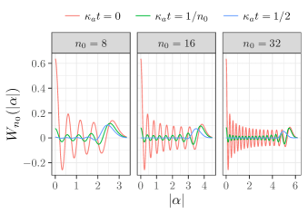
Figure 12: Radial part of the Wigner function for different initial Fock states $\ket{n_{0}}$.

On the contrary, this does not correspond to a fast decoherence over coherent states. Since the Fock states have no definite phase, it is natural to look for a mixture of coherent states which is uniform in its phase distribution. A natural expression for any state without phase preference would thus be:

$$\rho=\int q(n_{0})\ket{\sqrt{n_{0}}\mathrm{e}^{\mathrm{i}\theta}}\!\bra{\sqrt{n_{0}}\mathrm{e}^{\mathrm{i}\theta}}\,\mathrm{d}\theta\mathrm{d}n_{0}\,.$$ (46)

We can easily show that

$$\rho=\sum_{n}\int q(n_{0})P_{n_{0}}(n)\,\mathrm{d}n_{0}\ket{n}\!\bra{n}\,,$$ (47)

where $P_{n_{0}}$ is the Poisson distribution of rate $n_{0}$. The resulting distribution over Fock states thus has a variance equal to its mean. This is approximately the case for the binomial distribution only when $p\simeq 0$.

As such, the timescale to have decoherence over coherent states from an initial Fock states is $1/\kappa_{a}$, the same as the relaxation scale. This situation is actually similar as the one for coherent states in respect to the $L_{n}$ dynamics: the short timescale governs the spreading in phase space, while the long timescale governs the decoherence between the Fock states. This is summarized on Table 1.

References

- Zurek (2003) W. Zurek, Rev. Mod. Phys. 75 (2003).
- Zurek (2008) W. Zurek, arXiv preprint arXiv:0707.2832 (2008).
- Zurek (2009) W. Zurek, Nature Physics 5, 181-188 (2009).
- Zwolak et al. (2009) M. Zwolak, H. Quan, and W. H. Zurek, arXiv preprint arXiv:0911.4307 (2009).
- Riedel and Zurek (2010) C. J. Riedel and W. H. Zurek, Physical review letters 105, 020404 (2010).
- Riedel and Zurek (2011) C. J. Riedel and W. H. Zurek, New Journal of Physics 13, 073038 (2011).
- Riedel et al. (2012) C. J. Riedel, W. H. Zurek, and M. Zwolak, New Journal of physics 14, 083010 (2012).
- Riedel et al. (2016) C. J. Riedel, W. H. Zurek, and M. Zwolak, Physical Review A 93, 032126 (2016).
- Brandão et al. (2015) F. G. Brandão, M. Piani, and P. Horodecki, Nature communications 6, 7908 (2015).
- Knott et al. (2018) P. A. Knott, T. Tufarelli, M. Piani, and G. Adesso, Physical review letters 121, 160401 (2018).
- Qi and Ranard (2020) X. Qi and D. Ranard, arXiv preprint arXiv:2001.01507 (2020).
- Arthurs and Kelly (1965) E. Arthurs and J. Kelly, The Bell System Technical Journal 44, 725 (1965).
- Briegel and Englert (1993) H.-J. Briegel and B.-G. Englert, Phys. Rev. A 47, 3311 (1993), URL https://link.aps.org/doi/10.1103/PhysRevA.47.3311.
- Torres (2014) J. M. Torres, Physical Review A 89, 052133 (2014).
- Torres et al. (2019) J. M. Torres, R. Betzholz, and M. Bienert, Journal of Physics A: Mathematical and Theoretical 52, 08LT02 (2019), URL https://doi.org/10.1088%2F1751-8121%2Faafffe.
- Neto et al. (2003) A. H. C. Neto, E. Novais, L. Borda, G. Zaránd, and I. Affleck, Physical review letters 91, 096401 (2003).
- Novais et al. (2005) E. Novais, A. H. Castro Neto, L. Borda, I. Affleck, and G. Zarand, Phys. Rev. B 72, 014417 (2005), URL https://link.aps.org/doi/10.1103/PhysRevB.72.014417.
- Bonzom et al. (2008) V. Bonzom, H. Bouzidi, and P. Degiovanni, The European Physical Journal D 47, 133 (2008).
- Jordan and Büttiker (2005) A. N. Jordan and M. Büttiker, Physical review letters 95, 220401 (2005).
- Ruskov et al. (2010) R. Ruskov, A. N. Korotkov, and K. Mølmer, Physical review letters 105, 100506 (2010).
- Hacohen-Gourgy et al. (2016) S. Hacohen-Gourgy, L. S. Martin, E. Flurin, V. V. Ramasesh, K. B. Whaley, and I. Siddiqi, Nature 538, 491 (2016).
- Essig et al. (2020) A. Essig, Q. Ficheux, T. Peronnin, N. Cottet, R. Lescanne, A. Sarlette, P. Rouchon, Z. Leghtas, and B. Huard, Multiplexed photon number measurement (2020), eprint 2001.03217.
- Haroche and Raimond (2013) S. Haroche and J.-M. Raimond, Exploring the quantum: atoms, cavities, and photons (Oxford University Press, USA, 2013).
- Nogues et al. (1999) G. Nogues, A. Rauschenbeutel, S. Osnaghi, M. Brune, J. Raimond, and S. Haroche, Nature 400, 239 (1999).
- Guerlin et al. (2007) C. Guerlin, J. Bernu, S. Deleglise, C. Sayrin, S. Gleyzes, S. Kuhr, M. Brune, J.-M. Raimond, and S. Haroche, Nature 448, 889 (2007).
- Caldeira and Leggett (1985) A. O. Caldeira and A. J. Leggett, Physical Review A 31, 1059 (1985).
- Dalibard et al. (1992) J. Dalibard, Y. Castin, and K. Mølmer, Phys. Rev. Lett. 68, 580 (1992), URL https://link.aps.org/doi/10.1103/PhysRevLett.68.580.
- Ficheux et al. (2018) Q. Ficheux, S. Jezouin, Z. Leghtas, and B. Huard, Nature communications 9, 1926 (2018).
- Havel (2003) T. F. Havel, Journal of Mathematical Physics 44, 534 (2003).
- Carmichael (1999) H. J. Carmichael, Statistical Methods in Quantum Optics 1: Master Equations and Fokker-Planck Equations, vol. 1 (Springer Science & Business Media, 1999).
- Arnol’d (2013) V. I. Arnol’d, Mathematical methods of classical mechanics, vol. 60 (Springer Science & Business Media, 2013).
- Wigner (1932) E. Wigner, Physical Review 40, 749 (1932).
- Ville (1948) J. Ville, Câbles et transmissions 2, 61 (1948).
- Flandrin (1998) P. Flandrin, Time-frequency/time-scale analysis, vol. 10 (Academic press, 1998).
- Kiefer et al. (2007) C. Kiefer, I. Lohmar, D. Polarski, and A. A. Starobinsky, Classical and Quantum Gravity 24, 1699 (2007).
- Riedel (2016) C. J. Riedel, Physical Review A 93, 012107 (2016).
- Gisin and Rigo (1995) N. Gisin and M. Rigo, Journal of Physics A: Mathematical and General 28, 7375 (1995).
- Busse and Hornberger (2009) M. Busse and K. Hornberger, Journal of Physics A: Mathematical and Theoretical 43, 015303 (2009).
- Diósi and Kiefer (2000) L. Diósi and C. Kiefer, Physical review letters 85, 3552 (2000).
- Rényi et al. (1961) A. Rényi et al., in Proceedings of the Fourth Berkeley Symposium on Mathematical Statistics and Probability, Volume 1: Contributions to the Theory of Statistics (The Regents of the University of California, 1961).
- Biscani et al. (2019) F. Biscani, D. Izzo, W. Jakob, GiacomoAcciarini, M. Märtens, M. C, A. Mereta, C. Kaldemeyer, S. Lyskov, G. Acciarini, et al., esa/pagmo2: pagmo 2.12.0 (2019), URL https://doi.org/10.5281/zenodo.3582877.
- Gill et al. (2005) P. E. Gill, W. Murray, and M. A. Saunders, SIAM review 47, 99 (2005).
- Perelomov (2012) A. Perelomov, Generalized coherent states and their applications (Springer Science & Business Media, 2012).