Stochastic Analysis of an Adaptive Cubic Regularisation Method under Inexact Gradient Evaluations and Dynamic Hessian Accuracy

Abstract

We here adapt an extended version of the adaptive cubic regularisation method with dynamic inexact Hessian information for nonconvex optimisation in [3] to the stochastic optimisation setting. While exact function evaluations are still considered, this novel variant inherits the innovative use of adaptive accuracy requirements for Hessian approximations introduced in [3] and additionally employs inexact computations of the gradient. Without restrictions on the variance of the errors, we assume that these approximations are available within a sufficiently large, but fixed, probability and we extend, in the spirit of [18], the deterministic analysis of the framework to its stochastic counterpart, showing that the expected number of iterations to reach a first-order stationary point matches the well known worst-case optimal complexity. This is, in fact, still given by $O(\epsilon^{-3/2})$, with respect to the first-order $\epsilon$ tolerance. Finally, numerical tests on nonconvex finite-sum minimisation confirm that using inexact first and second-order derivatives can be beneficial in terms of the computational savings.

1 Introduction

Adaptive Cubic Regularisation (ARC) methods are Newton-type procedures for solving unconstrained optimisation problems of the form

$$\min_{x\in\mathbb{R}^{n}}f(x),$$ (1.1)

in which $f:\mathbb{R}^{n}\rightarrow\mathbb{R}$ is a sufficiently smooth, bounded below and, possibly, nonconvex function. In the seminal work by [26] the iterative scheme of the method is based on the minimisation of a cubic model, relying on the Taylor series, for predicting the objective function values, and is a globally convergent second-order procedure. The main reason to consider the ARC framework in place of other globalisation strategies, such as Newton-type methods embedded into a linesearch or a trust-region scheme, lies on its optimal complexity. In fact, given the first-order $\epsilon$ tolerance and assuming Lipschitz continuity of the Hessian of the objective function, an $\epsilon$-approximate first-order stationary point is reached, in the worst-case, in at most $O(\epsilon^{-3/2})$ iterations, instead of the $O(\epsilon^{-2})$ bound gained by trust-region and linesearch methods [12, 17]. More in depth, an $(\epsilon,\epsilon_{H})$-approximate first- and second-order critical point is found in at most $O(\max(\epsilon^{-3/2},\epsilon_{H}^{-3}))$ iterations, where $\epsilon_{H}$ is the positive prefixed second-order optimality tolerance [16, 12, 14, 26]. We observe that, in [9] it has been shown that the bound $O(\epsilon^{-3/2})$ for computing an $\epsilon$-approximate first-order stationary point is optimal among methods operating on functions with Lipschitz continuous Hessian. Experimentally, second-order methods can be more efficient than first-order ones on badly scaled and ill-conditioned problems, since they take advantage of curvature information to easily escape from saddle points to search for local minima ([11, 12, 33]) and this feature is in practice quite robust to the use of inexact Hessian information. On the other hand, their per-iteration cost is expected to be higher than first-order procedures, due to the computation of the Hessian-vector products. Consequently, literature has recently focused on ARC variants with inexact derivative information, starting from schemes employing Hessian approximations [3, 21, 32] though conserving optimal complexity. ARC methods with inexact gradient and Hessian approximations and still preserving optimal complexity are given in [4, 18, 25, 33, 34, 35]. These approaches have mostly been applied to large-scale finite-sum minimisation problems

$$\min_{x\in\mathbb{R}^{n}}f(x)=\frac{1}{N}\sum_{i=1}^{N}{\varphi_{i}(x)},$$ (1.2)

widely used in machine learning applications. In this setting, the objective function $f$ is the mean of $N$ component functions $\varphi_{i}:\mathbb{R}^{n}\rightarrow\mathbb{R}$ and, hence, the evaluation of the exact derivatives might be, for larger values of $N$, computationally expensive. In the papers cited above the derivatives approximations are required to fulfil given accuracy requirements and are computed by random sampling. The size of the sample is determined as to satisfy the prescribed accuracy with a sufficiently large prefixed probability exploiting the operator Bernstein inequality for tensors (see [30]). To deal with the nondeterministic aspects of these algorithms, in [18, 35] probabilistic models are considered and it is proved that, in expectation, optimal complexity applies as in the deterministic case; in [3, 4, 21, 32, 34] high probability results are given and it is shown that the optimal complexity result is restored in probability. Nevertheless, this latter analysis does not provide information on the behaviour of the method when the desired accuracy levels in derivatives approximations are not fulfilled. With the aim of filling this gap, we here perform the stochastic analysis of the framework in [3], where approximated Hessians are employed. To make the method more general, inexactness is allowed in first-order information, too. The analysis aims at bounding the expected number of iterations required by the algorithm to reach a first-order stationary point, under the assumption that gradient and Hessian approximations are available within a sufficiently large, but fixed, probability, recovering optimal complexity in the spirit of [18].

The rest of the paper is organised as follows. In section 1.1 we briefly survey the related works and in section 1.2 we summarise our contributions. In Section 2 we introduce a stochastic ARC algorithm with inexact gradients and dynamic Hessian accuracy and state the main assumptions on the stochastic process induced by the algorithm. Relying on several existing results and deriving some additional outcomes, Section 3 is then devoted to perform the complexity analysis of the framework, while Section 4 proposes a practical guideline to apply the method for solving finite-sum minimisation problems. Numerical results for nonconvex finite-sum minimisation problems are discussed in Section 5 and concluding remarks are finally given in Section 6. Notations. The Euclidean vector and matrix norm is denoted as $\|\cdot\|$. Given the scalar or vector or matrix $v$, and the non-negative scalar $\chi$, we write $v=O(\chi)$ if there is a constant $g$ such that $\|v\|\leq g\chi$. Given any set ${\cal{S}}$, $|{\cal{S}}|$ denotes its cardinality. As usual, $\mathbb{R}^{+}$ denotes the set of positive real numbers.

1.1 Related works

The interest in ARC methods with inexact derivatives has been steadily increasing. We are here interested in computable accuracy requirements for gradient and Hessian approximations, preserving optimal complexity of these procedures. Focusing on the Hessian approximation, in [16] it has been proved that optimal complexity is conserved provided that, at each iteration $k$, the Hessian approximation $\overline{\nabla^{2}f}(x_{k})$ satisfies

$$\|(\overline{\nabla^{2}f}(x_{k})-\nabla^{2}f(x_{k}))s_{k}\|\leq\chi\|s_{k}\|^{2},$$ (1.3)

where ${\nabla^{2}f}(x_{k})$ denotes the true Hessian at $x_{k}$. The method in [25], specifically designed to minimise finite-sum problems, assume that $\overline{\nabla^{2}f}(x_{k})$ satisfies

$$\|\overline{\nabla^{2}f}(x_{k})-\nabla^{2}f(x_{k})\|\leq\chi\|s_{k}\|$$ (1.4)

with $\chi$ a positive constant, leading to (1.3). Unfortunately, the upper bound in use depends on the steplength $\|s_{k}\|$ which is unknown when forming the Hessian approximation $\overline{\nabla^{2}f}(x_{k})$. Finite-differences versions of ARC method have been investigated in [13]. The Hessian approximation satisfies (1.4) and its computation requires an inner-loop to meet the accuracy requirement. This mismatch is circumvented, in practical implementations of the method in [25], by taking the step length at the previous iteration. Hence, this approach is unreliable when the norm of the step varies significantly from an iteration to the other, as also noticed in the numerical tests of [3]. To overcome this practical issue, Xu and others replace in [32] the accuracy requirement (1.4) with

$$\|\overline{\nabla^{2}f}(x_{k})-\nabla^{2}f(x_{k})\|\leq\chi\epsilon,$$ (1.5)

where $\epsilon$ is the first-order tolerance. This provides them with $\|(\overline{\nabla^{2}f}(x_{k})-\nabla^{2}f(x_{k}))s_{k}\|\leq\chi\epsilon\|s_{k}\|$, used to prove optimal complexity. In this situation, the estimate $\overline{\nabla^{2}f}(x_{k})$ is practically computable, independently of the step length, but at the cost of a very restrictive accuracy requirement (it is defined in terms of the $\epsilon$ tolerance) to fulfil at each iteration of the method. We further note that, in [31], optimal complexity results for a cubic regularisation method employing the implementable condition

$$\|\overline{\nabla^{2}f}(x_{k})-\nabla^{2}f(x_{k})\|\leq\chi\|s_{k-1}\|$$ (1.6)

are given under the assumption that the constant regularisation parameter is greater than the Hessian Lipschitz constant. Then, the knowledge of the Lipschitz constant is assumed. Such an assumption can be quite stringent, especially when minimising nonconvex objective functions. On the contrary, adaptive cubic regularisation frameworks get rid of the Lipschitz constant, trying to overestimate it by an adaptive procedure that is well defined provided that the approximated Hessian is accurate enough. To our knowledge, accuracy requirements depending on the current step, as those in (1.3)-(1.5), are needed to prove that the step acceptance criterion is well-defined and the regularisation parameter is bounded above.

Regarding the gradient approximation, the accuracy requirement in [13, 25] has the following form

$$\|\overline{\nabla f}(x_{k})-\nabla f(x_{k})\|\leq\mu\|s_{k}\|^{2},$$ (1.7)

where $\overline{\nabla f}(x_{k})$ denotes the gradient approximation and $\mu$ is a positive constant. Then, the accuracy requirement depends on the norm of the step again.

In [34], as for the Hessian approximation, in order to get rid of the norm of the step, a very tight accuracy requirement in used as the absolute error has to be of the order of $\epsilon^{2}$ at each iteration, i.e.

$$\|\overline{\nabla f}(x_{k})-\nabla f(x_{k})\|\leq\mu\epsilon^{2}.$$ (1.8)

As already noticed, in [32, 34], a complexity analysis in high probability is carried out in order to cover the situation where accuracy requirements (1.5) and (1.8) are satisfied only with a sufficiently large probability. While the behaviour of cubic regularisation approaches employing approximated derivatives is analysed in expectation in [18], assuming that (1.3) and (1.7) are satisfied with high probability. In the finite-sum minimisation context, accuracy requirements (1.3), (1.4) and (1.7) can be enforced with high probability by subsampling via an inner iterative process. Namely, the approximated derivative is computed using a predicted accuracy, the step $s_{k}$ is computed and, if the predicted accuracy is larger than the required accuracy, the predicted accuracy is progressively decreased (and the sample size progressively increased) until the accuracy requirement is satisfied.

The cubic regularisation variant proposed in [3] employs exact gradient and ensures condition (1.3), avoiding the above vicious cycle, requiring that

$$\|\overline{\nabla^{2}f}(x_{k})-\nabla^{2}f(x_{k})\|\leq c_{k},$$ (1.9)

where the guideline for choosing $c_{k}$ is as follows:

$$c_{k}\leq\left\{\begin{array}[]{ll}c,\quad c>0,\qquad\qquad~{}~{}~{}\mbox{if }\ \ \|s_{k}\|\geq 1,\\ \alpha(1-\beta)\|\nabla f(x_{k})\|,\quad\mbox{if }\ \ \|s_{k}\|<1,\end{array}\right.$$ (1.10)

with $0\leq\alpha<\frac{2}{3}$ and $0<\beta<1$. Note that, for a sufficiently large constant $c$, the accuracy requirement $c_{k}$ can be less stringent than $\epsilon$ when $\|s_{k}\|\geq 1$ or, otherwise, as long as $\alpha(1-\beta)\|\nabla f(x_{k})\|>\epsilon$. Despite condition (1.10) still involves the norm of the step, the accuracy requirement (1.9) can be implemented without requiring an inner loop (see, [3] and Algorithm 2).

We finally mention that regularisation methods employing inexact derivatives and also inexact function values are proposed in [4] and the complexity analysis carried out covers arbitrary optimality order and arbitrary degree of the available approximate derivatives. Also in this latter approach, the accuracy requirement in derivatives approximation depends on the norm of the step and an inner loop is needed in order to increase the accuracy and meet the accuracy requirements. A different approach based on the Inexact Restoration framework is given in [8] where, in the context of finite-sums problems, the sample size rather than the approximation accuracy is adaptively chosen.

1.2 Contributions

In light of the related works the main contributions of this paper are the following:

• We generalise the method given in [3]. In particular, we kept the practical adaptive criterion (1.9), which is implemented without including an inner loop, allowing inexactness in the gradient as well. Namely, inspired by [4], we require that the gradient approximation satisfies the following relative implicit condition:

  $$\|\overline{\nabla f}(x_{k})-\nabla f(x_{k})\|\leq\zeta_{k}\|\overline{\nabla}f(x_{k})\|^{2},$$ (1.11)

  where $\zeta_{k}$ is an iteration-dependent nonnegative parameter. Unlike [18] and [25] (see (1.7)), this latter condition does not depend on the norm of the step. Thus, its practical implementation calls for an inner loop that can be performed before the step computation and extra-computations of the step are not needed. A detailed description of a practical implementation of this accuracy requirement in subsampling scheme for finite-sum minimisation is given in Section 4.

• We assume that the accuracy requirements (1.9) and (1.11) are satisfied with high probability and we perform, in the spirit of [18], the stochastic analysis of the resulting method, showing that the expected number of iterations needed to reach an $\epsilon$-approximate first-order critical point is, in the worst-case, of the order of $\epsilon^{-3/2}$. This analysis also applies to the method given in [3].

2 A stochastic cubic regularisation algorithm with inexact derivatives evaluations

Before introducing our stochastic algorithm, we consider the following hypotheses on $f$.

Assumption 2.1.

With reference to problem (1.1), the objective function $f$ is assumed to be:

• bounded below by $f_{low}$, for all $x\in\hbox{I\hskip-2.0ptR}^{n}$;

• twice continuously differentiable, i.e. $f\in\mathcal{C}^{2}(\mathbb{R}^{n})$;

Moreover,

• the Hessian is globally Lipschitz continuous with Lipschitz constant $L_{H}>0$, i.e.,

  $$\qquad\|\nabla^{2}f(x)-\nabla^{2}f(y)\|\leq L_{H}\|x-y\|,$$ (2.1)

  for all $x$, $y\in\mathbb{R}^{n}$.

The iterative method we are going to introduce is, basically, the stochastic counterpart of an extension of the one proposed in [3], based on first and second-order inexact information. More in depth at iteration $k$, given the trial step $s$, the value of the objective function at $x_{k}+s$ is predicted by mean of a cubic model $m_{k}(x_{k},s,\sigma_{k})$ defined in terms of an approximate Taylor expansion of $f$ centered at $x_{k}$ with increment $s$, truncated to the second order, namely

$$m_{k}(x_{k},s,\sigma_{k})=f(x_{k})+\overline{\nabla f}(x_{k})^{T}s+\frac{1}{2}s^{T}\overline{\nabla^{2}f}(x_{k})s+\frac{\sigma_{k}}{3}\|s\|^{3}\stackrel{{\scriptstyle\rm def}}{{=}}\overline{T}_{2}(x_{k},s)+\frac{\sigma_{k}}{3}\|s\|^{3},$$ (2.2)

in which both the gradient $\overline{\nabla f}(x_{k})$ and the Hessian matrix $\overline{\nabla^{2}f}(x_{k})$ represent approximations of $\nabla f(x_{k})$ and $\nabla^{2}f(x_{k})$, respectively. According to the basic ARC framework in [15], the main idea is to approximately minimise, at each iteration, the cubic model and to adaptively search for a regulariser $\sigma_{k}$ such that the following overestimation property is satisfied:

$$f(x_{k}+s)\leq m_{k}(x_{k},s,\sigma_{k}),$$

in which $s$ denotes the approximate minimiser of $m_{k}(x_{k},s,\sigma_{k})$. Within these requirements, it follows that

$$f(x_{k})=m_{k}(x_{k},0,\sigma_{k})\geq m_{k}(x_{k},s,\sigma_{k})\geq f(x_{k}+s),$$

so that the objective function is not increased when moving from $x_{k}$ to $x_{k}+s$. To get more insight, the cubic model (2.2) is approximately minimised in the sense that the minimiser $s_{k}$ satisfies

$$m_{k}(x_{k},s_{k},\sigma_{k})<m_{k}(x_{k},0,\sigma_{k}),$$ (2.3)

$$\|\nabla_{s}m_{k}(x_{k},s_{k},\sigma_{k})\|\leq\beta_{k}\|\overline{\nabla f}(x_{k})\|,$$ (2.4)

for all $k\geq 0$ and some $0\leq\beta_{k}\leq\beta$, $\beta\in[0,1)$. Practical choices for $\beta_{k}$ are, for instance, $\beta_{k}=\beta\min\left(1,\frac{\|s_{k}\|^{2}}{\|\overline{\nabla f}(x_{k})\|}\right)$ or $\beta_{k}=\beta\min(1,\|s_{k}\|)$ (see, e.g., [3]), leading to

$$\|\nabla_{s}m_{k}(x_{k},s_{k},\sigma_{k})\|\leq\beta\min\left(\|s_{k}\|^{2},\|\overline{\nabla f}(x_{k})\|\right),$$ (2.5)

and

$$\|\nabla_{s}m_{k}(x_{k},s_{k},\sigma_{k})\|\leq\beta\min(1,\|s_{k}\|)\|\overline{\nabla f}(x_{k})\|,$$ (2.6)

respectively. We notice that, if the overestimation property $f(x_{k}+s)\leq m_{k}(x_{k},s,\sigma_{k})$ is satisfied, the requirement (2.3) implies that $f(x_{k})=m_{k}(x_{k},0,\sigma_{k})>m_{k}(x_{k},s,\sigma_{k})\geq f(x_{k}+s)$, resulting in a decrease of the objective. The trial point $x_{k}+s_{k}$ is then used to compute the relative decrease [7]

$$\rho_{k}=\frac{f(x_{k})-f(x_{k}+s_{k})}{\overline{T}_{2}(x_{k},0)-\overline{T}_{2}(x_{k},s_{k})}.$$ (2.7)

If $\rho_{k}\geq\eta$, with $\eta\in(0,1)$ a prescribed decrease fraction, then the trial point is accepted, the iteration is declared successful, the regularisation parameter is decreased by a factor $\gamma$ and we go on recomputing the approximate model at the updated iterate; otherwise, an unsuccessful iteration occurs: the point $x_{k}+s_{k}$ is rejected, the regulariser is increased by a factor $\gamma$, a new approximate model at $x_{k}$ is computed and a new trial step $s_{k}$ is recomputed. At each iteration, the model $m_{k}(x_{k},s,\sigma_{k})$ involved relies on inexact quantities, that can be considered as realisations of random variables. Hereafter, all random quantities are denoted by capital letters, while the use of small letters is reserved for their realisations. In particular, let us denote a random model at iteration $k$ as $M_{k}$, while we use the notation $m_{k}=M_{k}(\omega)$ for its realisation, with $\omega$ a random sample taken from a context-dependent probability space $\Omega$. In particular, we denote by $\overline{\nabla f}(X_{k})$ and $\overline{\nabla^{2}f}(X_{k})$ the random variables for $\overline{\nabla f}(x_{k})$ and $\overline{\nabla^{2}f}(x_{k})$, respectively. Consequently, the iterates $X_{k}$, as well as the regularisers $\Sigma_{k}$ and the steps $S_{k}$ are the random variables such that $x_{k}=X_{k}(\omega)$, $\sigma_{k}=\Sigma_{k}(\omega)$ and $s_{k}=S_{k}(\omega)$.

The focus of this paper is to derive the expected worst-case complexity bound to approach a first-order optimality point, that is, given a tolerance $\epsilon\in(0,1)$, the number of steps $\overline{k}$ (in the worst-case) such that an iterate $x_{\overline{k}}$ satisfying

$$\|\nabla f(x_{\overline{k}})\|\leq\epsilon$$

is reached. To this purpose, after the description of the algorithm, we state the main definitions and hypotheses needed to carry on with the analysis up to the complexity result. Our algorithm is reported below.

Algorithm 2.1: Stochastic ARC algorithm with inexact gradient and dynamic Hessian accuracy
Step 0: Initialisation. An initial point $x_{0}\in\mathbb{R}^{n}$ and an initial regularisation parameter $\sigma_{0}>0$ are given. The constants $\beta$, $\alpha$, $\eta$, $\gamma$, $\sigma_{\textrm{min}}$ and $c$ are also given such that $\displaystyle 0<\beta<1,~{}\alpha\in\left[0,\displaystyle\frac{2}{3}\right),~{}\sigma_{\min}\in(0,\sigma_{0}],~{}0<\eta<\frac{2-3\alpha}{2},~{}\gamma>1,~{}c>0.$ (2.8) Compute $f(x_{0})$ and set $k=0$, ${\rm flag}=1$. Step 1: Gradient approximation. Compute an approximate gradient $\overline{\nabla f}(x_{k})$ Step 2: Hessian approximation (model costruction). If ${\rm flag}=1$ set $c_{k}=c$, else set $c_{k}=\alpha(1-\beta)\|\overline{\nabla f}(x_{k})\|$.
Compute an approximate Hessian $\overline{\nabla^{2}f}(x_{k})$ that satisfies condition (1.9) with a prefixed probability. Form the model $m_{k}(x_{k},s,\sigma_{k})$ defined in (2.2). Step 3: Step calculation. Choose $\beta_{k}\leq\beta$. Compute the step $s_{k}$ satisfying (2.3)-(2.4). Step 4: Check on the norm of the trial step. If $\|s_{k}\|<1$ and ${\rm flag}=1$ and $c>\alpha(1-\beta)\|\overline{\nabla f}(x_{k})\|$ set $x_{k+1}=x_{k}$, $\sigma_{k+1}=\sigma_{k}$, ${\rm flag}=0$ (unsuccessful iteration) set $k=k+1$ and go to Step $1$. Step 5: Acceptance of the trial point and parameters update. Compute $f(x_{k}+s_{k})$ and the relative decrease defined in (2.7). If $\rho_{k}\geq\eta$ define $x_{k+1}=x_{k}+s_{k}$, set $\sigma_{k+1}=\max[\sigma_{\min},\frac{1}{\gamma}\sigma_{k}]$. (successful iteration) If $\|s_{k}\|\geq 1$ set ${\rm flag}=1$, otherwise set ${\rm flag}=0$. else define $x_{k+1}=x_{k}$, $\sigma_{k+1}=\gamma\sigma_{k}.\quad$ (unsuccessful iteration) Set $k=k+1$ and go to Step $1$.

Some comments on this algorithm are useful at this stage. We first note that the Algorithm 2 generates a random process

$$\{X_{k},S_{k},M_{k},\Sigma_{k},C_{k}\},$$ (2.9)

where $C_{k}=c_{k}(\omega)$ refers to the random variable for the dynamic Hessian accuracy $c_{k}$, that is adaptively defined in Step 2 of Algorithm 2. Since its definition relies on random quantities, $c_{k}$ constitutes a random variable too. We recall that, in the deterministic counterpart given in [3], the Hessian approximation $\overline{\nabla^{2}f}(x_{k})$ computed at iteration $k$ has to satisfy the absolute accuracy requirement (1.9). Here, this condition is assumed to be satisfied only with a certain probability (see, e.g., Assumption 2.2).

The main goal is thus to prove that, if $M_{k}$ is sufficiently accurate with a sufficiently high probability conditioned to the past, then the stochastic process preserves the expected optimal complexity. To this scope, the next section is devoted to state the basic probabilistic accuracy assumptions and definitions. In what follows, we use the notation $\mathbb{E}[X]$ to indicate the expected value of a random variable $X$. In addition, given a random event $A$, $Pr(A)$ denotes the probability of $A$, while $\mathbbm{1}_{A}$ refers to the indicator of the random event $A$ occurring (i.e. $\mathbbm{1}_{A}(a)=1$ if $a\in A$, otherwise $\mathbbm{1}_{A}(a)=0$). The notation $A^{c}$ indicates the complement of the event $A$.

2.1 Main assumptions on the stochastic ARC algorithm

For $k\geq 0$, to formalise the conditioning on the past, let $\mathcal{F}_{k-1}^{M}$ denote the $\hat{\sigma}$-algebra induced by the random variables $M_{0}$, $M_{1}$,…, $M_{k-1}$, with $\mathcal{F}_{-1}^{M}=\hat{\sigma}(x_{0})$.
We first consider the following definitions for measuring the accuracy of the model estimates.

Definition 2.1 (Accurate model).

A sequence of random models $\{M_{k}\}$ is said to be $p$-probabilistically sufficiently accurate for Algorithm 2, with respect to the corresponding sequence $\{X_{k},S_{k},\Sigma_{k},C_{k}\}$, if the event $I_{k}=I_{k}^{(1)}\cap I_{k}^{(2)}\cap I_{k}^{(3)}$, with

$$I_{k}^{(1)} = \left\{\|\overline{\nabla f}(X_{k})-\nabla f(X_{k})\|\leq\kappa(1-\beta)^{2}\left(\frac{\|\overline{\nabla f}(X_{k})\|}{\Sigma_{k}}\right)^{2},\quad\kappa>0\right\},$$ (2.10)

$$I_{k}^{(2)} = \left\{\|\overline{\nabla^{2}f}(X_{k})-\nabla^{2}f(X_{k})\|\leq C_{k}\right\},$$ (2.11)

$$I_{k}^{(3)} = \left\{\|\overline{\nabla f}(x_{k})\|\leq\kappa_{g},\quad\|\overline{\nabla^{2}f}(x_{k})\|\leq\kappa_{B},\quad\quad\kappa_{g}>0,~{}\kappa_{B}>0\right\},$$ (2.12)

satisfies

$$Pr(I_{k}|\mathcal{F}_{k-1}^{M})=\mathbb{E}[\mathbbm{1}_{I_{k}}|\mathcal{F}_{k-1}^{M}]\geq p.$$ (2.13)

What follows is an assumption regarding the nature of the stochastic information used by Algorithm 2.

Assumption 2.2.

We assume that the sequence of random models $\{M_{k}\}$, generated by Algorithm 2, is $p$-probabilistically sufficiently accurate for some sufficiently high probability $p\in(0,1]$.

3 Complexity analysis of the algorithm

For a given level of tolerance $\epsilon$, the aim of this section is to derive a bound on the expected number of iterations $\mathbb{E}[N_{\epsilon}]$ which is needed, in the worst-case, to reach an $\epsilon$-approximate first-order stationary point. Specifically, $N_{\epsilon}$ denotes a random variable corresponding to the number of steps required by the process until $\|\nabla f(X_{k})\|\leq\epsilon$ occurs for the first time, namely

$$N_{\epsilon}=\inf\{k\geq 0~{}|~{}\|\nabla f(X_{k})\|\leq\epsilon\};$$ (3.14)

indeed, $N_{\epsilon}$ can be seen as a stopping time for the stochastic process generated by Algorithm 2 (see [10, Definition 2.1]). The analysis follows the path of [18], but some results need to be proved as for the adopted accuracy requirements for gradient and Hessian and failures in the sense of Step 4. It is preliminarly useful to sum up a series of existing lemmas from [18] and [3] and to derive some of their suitable extensions, which will be of paramount importance to perform the complexity analysis of our stochastic method. These lemmas are recalled in the following subsection.

3.1 Existing and preliminary results

We observe that each iteration $k$ of Algorithm 2 such that $\mathbbm{1}_{I_{k}}=1$ corresponds to an iteration of the ARC Algorithm $3.1$ in [3], before termination, except for the fact that in Algorithm 2 the model (2.2) is defined not only using inexact Hessian information, but also considering an approximate gradient. In particular, the nature of the accuracy requirement for the gradient approximation given by (2.10) is different from the one for the Hessian approximation, namely (2.11). In fact, a realisation $c_{k}$ of the upper bound $C_{k}$ in (2.11), needed to obtain an approximate Hessian $\overline{\nabla^{2}f}(x_{k})$, is determined by the mechanism of the algorithm and is available when forming the Hessian approximation $\overline{\nabla^{2}f}(x_{k})$. On the other hand, (2.10) is an implicit condition and can be practically gained computing the gradient approximation within a prescribed absolute accuracy level, that is eventually reduced to recompute the inexact gradient $\overline{\nabla f}(x_{k})$; but, in contrast with [18, Algorithm $4.1$], without additional step computation, which is performed only once per iteration at Step $3$ of Algorithm 2. We will see that, for any realisation of the algorithm, if the model is accurate, i.e. $\mathbbm{1}_{I_{k}}=1$, then there exist $\delta\geq 0$ and $\xi_{k}>0$ such that

$$\|(\overline{\nabla f}(x_{k})-\nabla f(x_{k}))s_{k}\|\leq\delta\|s_{k}\|^{3},\qquad\|(\overline{\nabla^{2}f}(x_{k})-\nabla^{2}f(x_{k}))s_{k}\|\leq\xi_{k}\|s_{k}\|^{2},$$

which will be fundamental to recover optimal complexity. At this regard, let us consider the following definitions and state the lemma below.

Definition 3.1.

With reference to Algorithm 2, for all $0\leq k\leq l$, $l\in\{0,...,N_{\epsilon}-1\}$, we define the events

• $\mathcal{S}_{k}=\{\textrm{iteration~{}}k~{}\textrm{is successful}\}$;

• $\mathcal{U}_{k,1}=\{\textrm{iteration~{}}k~{}\textrm{is unsuccessful}~{}\textrm{in~{}the~{}sense~{}of~{}Step}~{}5\}$;

• $\mathcal{U}_{k,2}=\{\textrm{iteration~{}}k~{}\textrm{is unsuccessful}~{}\textrm{in~{}the~{}sense~{}of~{}Step}~{}4\}$.

We underline that if $k\in{\cal U}_{k,1}$ then $\rho_{k}<\eta$, while $k\in{\cal U}_{k,2}$ if and only if $\|s_{k}\|<1$, ${\rm flag}=1$ and $c>\alpha(1-\beta)\|\overline{\nabla f}(x_{k})\|$. Moreover, if $\rho_{k}<\eta$ and a failure in Step 4 does not occur, then $k\in{\cal U}_{k,1}$.

Lemma 3.1.

Consider any realisation of Algorithm 2. Then, at each iteration $k$ such that $\mathbbm{1}_{I_{k}^{(1)}\cap I_{k}^{(3)}}=1$ (accurate gradient and bounded inexact derivatives) we have $$\|\overline{\nabla f}(x_{k})-\nabla f(x_{k})\|\leq\delta\|s_{k}\|^{2},\qquad\delta\stackrel{{\scriptstyle\rm def}}{{=}}\kappa\left(\frac{\kappa_{B}}{\sigma_{\min}}+1\right)\max\left[\frac{\kappa_{g}}{\sigma_{\min}},\frac{\kappa_{B}}{\sigma_{\min}}+1\right],$$ (3.15) and, thus, $\displaystyle\|(\overline{\nabla f}(x_{k})-\nabla f(x_{k}))s_{k}\|\leq\delta\|s_{k}\|^{3}.$ (3.16)

Proof.

Let us consider $k$ such that $\mathbbm{1}_{I_{k}^{(1)}\cap I_{k}^{(3)}}=1$. Using (2.4) we obtain

$$\beta\|\overline{\nabla f}(x_{k})\| \geq \|\nabla_{s}m(x_{k},s_{k},\sigma_{k})\|=\left\|\,\overline{\nabla f}(x_{k})+\overline{\nabla^{2}f}(x_{k})s_{k}+\sigma_{k}s_{k}\|s_{k}\|\,\right\|$$ (3.17)

$$\geq \|\overline{\nabla f}(x_{k})\|-\|\overline{\nabla^{2}f}(x_{k})\|\,\|s_{k}\|-\sigma_{k}\|s_{k}\|^{2}.$$

We can then distinguish between two different cases. If $\|s_{k}\|\geq 1$, from (3.17) and (2.12) we have that

$$\beta\|\overline{\nabla f}(x_{k})\|\geq\|\overline{\nabla f}(x_{k})\|-\|\overline{\nabla^{2}f}(x_{k})\|\,\|s_{k}\|^{2}-\sigma_{k}\|s_{k}\|^{2}\geq\|\overline{\nabla f}(x_{k})\|-(\kappa_{B}+\sigma_{k})\|s_{k}\|^{2}$$

which is equivalent to

$$\|s_{k}\|^{2}\geq\frac{(1-\beta)\|\overline{\nabla f}(x_{k})\|}{\kappa_{B}+\sigma_{k}}.$$

Consequently, by (2.10) and (2.12)

$$\|\overline{\nabla f}(x_{k})-\nabla f(x_{k})\| \leq \kappa\left(\frac{1-\beta}{\sigma_{k}}\right)^{2}\|\overline{\nabla f}(x_{k})\|^{2}\leq\frac{\kappa\kappa_{g}(1-\beta)^{2}\|\overline{\nabla f}(x_{k})\|}{\sigma_{k}^{2}\|s_{k}\|^{2}}\|s_{k}\|^{2}$$ (3.18)

$$\leq \kappa\kappa_{g}(1-\beta)\frac{\kappa_{B}+\sigma_{k}}{\sigma_{k}^{2}}\|s_{k}\|^{2}\leq\kappa\frac{\kappa_{g}}{\sigma_{\min}}\left(\frac{\kappa_{B}}{\sigma_{\min}}+1\right)\|s_{k}\|^{2},$$

where in the last inequality we have used that $\beta\in(0,1)$ and $\sigma_{k}\geq\sigma_{min}$. If, instead, $\|s_{k}\|<1$, inequality (3.17) and (2.12) lead to

$$\beta\|\overline{\nabla f}(x_{k})\|\geq\|\overline{\nabla f}(x_{k})\|-\|\overline{\nabla^{2}f}(x_{k})\|\,\|s_{k}\|-\sigma_{k}\|s_{k}\|\geq\|\overline{\nabla f}(x_{k})\|-(\kappa_{B}+\sigma_{k})\|s_{k}\|,$$

obtaining that

$$\|s_{k}\|\geq\frac{(1-\beta)\|\overline{\nabla f}(x_{k})\|}{\kappa_{B}+\sigma_{k}}.$$ (3.19)

Hence, by squaring both sides in the above inequality and using (2.10), $\beta\in(0,1)$ and $\sigma_{k}\geq\sigma_{min}$, we obtain

$$\|\overline{\nabla f}(x_{k})-\nabla f(x_{k})\| \leq \kappa\left(\frac{1-\beta}{\sigma_{k}}\right)^{2}\|\overline{\nabla f}(x_{k})\|^{2}=\frac{\kappa(1-\beta)^{2}\|\overline{\nabla f}(x_{k})\|^{2}}{\sigma_{k}^{2}\|s_{k}\|^{2}}\|s_{k}\|^{2}$$ (3.20)

$$\leq \kappa\left(\frac{\kappa_{B}+\sigma_{k}}{\sigma_{k}}\right)^{2}\|s_{k}\|^{2}\leq\kappa\left(\frac{\kappa_{B}}{\sigma_{\min}}+1\right)^{2}\|s_{k}\|^{2}.$$

Inequality (3.15) then follows by virtue of (3.18) and (3.20), while (3.16) stems from (3.15) by means of the triangle inequality. ∎

The following Lemma is a slight modification of [3, Lemma 3.1].

Lemma 3.2.

Consider any realisation of Algorithm 2 and assume that $c\geq\alpha(1-\beta)\kappa_{g}$. Then, at each iteration $k$ such that $\mathbbm{1}_{I_{k}^{(2)}\cap I_{k}^{(3)}}(1-\mathbbm{1}_{\mathcal{U}_{k,2}})=1$ (successful or unsuccessful in the sense of Step $5$, with accurate Hessian and bounded inexact derivatives) we have $$\|\overline{\nabla^{2}f}(x_{k})-\nabla^{2}f(x_{k})\|\leq c_{k}\leq\xi_{k}\|s_{k}\|,\qquad\xi_{k}\stackrel{{\scriptstyle\rm def}}{{=}}\max[c,\alpha(\kappa_{B}+\sigma_{k})],$$ (3.21) and, thus, $\displaystyle\|(\overline{\nabla^{2}f}(x_{k})-\nabla^{2}f(x_{k}))s_{k}\|\leq\xi_{k}\|s_{k}\|^{2}.$ (3.22)

Proof.

Let us consider $k$ such that $\mathbbm{1}_{I_{k}^{(2)}\cap I_{k}^{(3)}}(1-\mathbbm{1}_{\mathcal{U}_{k,2}})=1$. Algorithm 2 ensures that, if $\|s_{k}\|\geq 1$, then $c_{k}=c$ or

$$c_{k}=\alpha(1-\beta)\|\overline{\nabla f}(x_{k})\|.$$ (3.23)

Trivially, (3.23), $\|s_{k}\|\geq 1$ and (2.12) give

$$\|\overline{\nabla^{2}f}(x_{k})-\nabla^{2}f(x_{k})\|\leq c_{k}\leq\max[c,\alpha(1-\beta)\|\overline{\nabla f}(x_{k})\|]\leq\max[c,\alpha(1-\beta)\kappa_{g}]\leq c\|s_{k}\|,$$ (3.24)

where we have considered the assumption $c\geq\alpha(1-\beta)\kappa_{g}$. On the other hand, Step $4$ guarantees the choice

$$c_{k}\leq\alpha(1-\beta)\|\overline{\nabla f}(x_{k})\|,$$ (3.25)

when $\|s_{k}\|<1$. In this case, inequality (3.19) still holds. Thus,

$$\|\overline{\nabla^{2}f}(x_{k})-\nabla^{2}f(x_{k})\|\leq c_{k}=\frac{c_{k}}{\|s_{k}\|}\|s_{k}\|\leq\frac{c_{k}(\kappa_{B}+\sigma_{k})}{(1-\beta)\|\overline{\nabla f}(x_{k})\|}\|s_{k}\|\leq\alpha(\kappa_{B}+\sigma_{k})\|s_{k}\|,$$ (3.26)

where the last inequality is due to (3.25). Finally, (3.24) and (3.26) imply (3.21), while (3.22) follows by (3.21) using the triangle inequality. ∎

The next lemma bounds the decrease of the objective function on successful iterations, irrespectively of the satisfaction of the accuracy requirements for gradient and Hessian approximations.

Lemma 3.3.

Consider any realisation of Algorithm 2. At each iteration $k$ we have $$\overline{T}_{2}(x_{k},0)-\overline{T}_{2}(x_{k},s_{k})>\frac{\sigma_{k}}{3}\|s_{k}\|^{3}\geq\frac{\sigma_{\min}}{3}\|s_{k}\|^{3}>0.$$ (3.27) Hence, on every successful iteration $k$: $$f(x_{k})-f(x_{k+1})>\eta\frac{\sigma_{k}}{3}\|s_{k}\|^{3}\geq\eta\frac{\sigma_{\min}}{3}\|s_{k}\|^{3}>0.$$ (3.28)

Proof.

We first notice that, by (2.3), we have that $\|s_{k}\|\neq 0$. Moreover, Lemma 2.1 in [7] coupled with (2.2) yields (3.27). The second part of the thesis is easily proved taking into account that, if $k$ is successful, then (3.27) implies

$$f(x_{k})-f(x_{k+1})\geq\eta(\overline{T}_{2}(x_{k},0)-\overline{T}_{2}(x_{k},s_{k}))>\eta\frac{\sigma_{k}}{3}\|s_{k}\|^{3}.$$

∎

As a corollary, because of the fact that $x_{k+1}=x_{k}$ on each unsuccessful iteration $k$, for any realisation of Algorithm 2 we have that

$$f(x_{k})-f(x_{k+1})\geq 0.$$

We now show that, if the model is accurate, there exists a constant $\overline{\sigma}>0$ such that an iteration is successful or unsuccessful in the sense of Step 4 ($\mathbbm{1}_{I_{k}}(1-\mathbbm{1}_{\mathcal{U}_{k,1}})=1$), whenever $\sigma_{k}\geq\overline{\sigma}$. In other words, it is an iteration at which the regulariser is not increased.

Lemma 3.4.

Let Assumption 2.1 (ii) hold. Let $\delta$ be given in (3.15), assume $c\geq\alpha(1-\beta)\kappa_{g}$ and the validity of (2.1). For any realisation of Algorithm 2, if the model is accurate and $$\sigma_{k}\geq\overline{\sigma}\stackrel{{\scriptstyle\rm def}}{{=}}\max\left[\frac{6\delta+3\alpha\kappa_{B}+L_{H}}{2(1-\eta)-3\alpha},\frac{6\delta+3c+L_{H}}{2(1-\eta)}\right]>0,$$ (3.29) then the iteration $k$ is successful or a failure in the sense of Step 4 occurs.

Proof.

Let us consider an iteration $k$ such that $\mathbbm{1}_{I_{k}}(1-\mathbbm{1}_{\mathcal{U}_{k,1}})=1$ and the definition of $\rho_{k}$ in (2.7). Assume that a failure in the sense of Step 4 does not occur. If $\rho_{k}-1\geq 0$, then iteration $k$ is successful by definition. We can thus focus on the case in which $\rho_{k}-1<0$. In this situation, the iteration $k$ is successful provided that $1-\rho_{k}\leq 1-\eta$. From (2.1) and the Taylor expansion of $f$ centered at $x_{k}$ with increment $s$ it first follows that

$$f(x_{k}+s)\leq f(x_{k})+\nabla f(x_{k})^{\top}s+\frac{1}{2}s^{\top}\nabla^{2}f(x_{k})s+\frac{L_{H}}{6}\|s\|^{3}.$$ (3.30)

Therefore, since $\mathbbm{1}_{I_{k}}=1$,

$$f(x_{k}+s_{k})-\overline{T}_{2}(x_{k},s_{k}) \leq (\nabla f(x_{k})-\overline{\nabla f}(x_{k}))^{\top}s_{k}+\frac{1}{2}s_{k}^{\top}(\nabla^{2}f(x_{k})-\overline{\nabla^{2}f}(x_{k}))s_{k}+\frac{L_{H}}{6}\|s_{k}\|^{3}$$ (3.31)

$$\leq \|\overline{\nabla f}(x_{k})-\nabla f(x_{k})\|\|s_{k}\|+\frac{1}{2}\|\overline{\nabla^{2}f}(x_{k})-\nabla^{2}f(x_{k})\|\|s_{k}\|^{2}+\frac{L_{H}}{6}\|s_{k}\|^{3}$$

$$\leq \left(\delta+\frac{L_{H}}{6}+\frac{\xi_{k}}{2}\right)\|s_{k}\|^{3},$$

where we have used (3.15) and (3.21). Thus, by (3.31) and (3.27),

$$1-\rho_{k}=\frac{f(x_{k}+s_{k})-\overline{T}_{2}(x_{k},s_{k})}{\overline{T}_{2}(x_{k},0)-\overline{T}_{2}(x_{k},s_{k})}<\frac{\left(6\delta+3\xi_{k}+L_{H}\right)\|s_{k}\|^{3}}{2\sigma_{k}\|s_{k}\|^{3}}=\frac{6\delta+3\xi_{k}+L_{H}}{2\sigma_{k}}.$$

Depending on the maximum in the definition of $\xi_{k}$ in (3.21), two different cases can then occur. If $\xi_{k}=c$, $1-\rho_{k}\leq 1-\eta$, provided that

$$\sigma_{k}\geq\frac{6\delta+3c+L_{H}}{2(1-\eta)}.$$

Otherwise, if $c<\alpha(\kappa_{B}+\sigma_{k})$, so that $\xi_{k}=\alpha(\kappa_{B}+\sigma_{k})$, then

$$1-\rho_{k}<\frac{6\delta+3\alpha(\kappa_{B}+\sigma_{k})+L_{H}}{2\sigma_{k}}\leq 1-\eta,$$

provided that

$$\sigma_{k}\geq\frac{6\delta+3\alpha\kappa_{B}+L_{H}}{2(1-\eta)-3\alpha}.$$

In conclusion, iteration $k$ is successful if (3.29) holds. Note that $\overline{\sigma}$ is a positive lower bound for $\sigma_{k}$ because of the ranges for the values of $\eta$ and $\alpha$ in (2.8). ∎

Using some of the results from the proof of the previous lemma, we can now prove the following, giving a crucial relation between the step length $\|s_{k}\|$ and the true gradient norm $\|\nabla f(x_{k}+s_{k})\|$ at the next iteration.

Lemma 3.5.

Let Assumption 2.1 (ii)-(iii) hold and assume $c\geq\alpha(1-\beta)\kappa_{g}$. For any realisation of Algorithm 2, at each iteration $k$ such that $\mathbbm{1}_{I_{k}}(1-\mathbbm{1}_{\mathcal{U}_{k,2}})=1$ (accurate in which the iteration is successful or a failure in the sense of Step 5 occurs), we have $$\|s_{k}\|\geq\sqrt{\nu_{k}\|\nabla f(x_{k}+s_{k})\|},$$ (3.32) for some positive $\nu_{k}$, whenever $s_{k}$ satisfies (2.5). Moreover, (3.32) holds even in case $s_{k}$ satisfies (2.6) provided that there exists $L_{g}>0$ such that $$\|\nabla f(x)-\nabla f(y)\|\leq L_{g}\|x-y\|,$$ (3.33) for all $x$, $y\in\mathbb{R}^{n}$.

Proof.

Let us consider an iteration $k$ such that $\mathbbm{1}_{I_{k}}(1-\mathbbm{1}_{\mathcal{U}_{k,2}})=1$. From the Taylor series of $\nabla f(x)$ centered at $x_{k}$ with increment $s$, and the definition of the model (2.2), proceeding as in the proof of Lemma 4.1 in [3] we obtain

$$\|\nabla f(x_{k}+s_{k})-\nabla_{s}\overline{T}_{2}(x_{k}+s_{k})\| \leq \|\nabla f(x_{k})-\overline{\nabla f}(x_{k})\|+\|(\nabla^{2}f(x_{k})-\overline{\nabla^{2}f}(x_{k}))s_{k}\|$$ (3.34)

$$~{}~{}~{}+ \int_{0}^{1}\|\nabla^{2}f(x_{k}+\tau s)-\nabla^{2}f(x_{k})\|\|s_{k}\|\,d\tau$$

$$\leq \left(\delta+\xi_{k}+\frac{L_{H}}{2}\right)\|s_{k}\|^{2},$$

where we have used (3.15), (3.22) and (2.1). Moreover, since $\nabla_{s}m(x_{k},s_{k},\sigma_{k})=\nabla_{s}\overline{T}_{2}(x_{k},s_{k})+\sigma_{k}\|s_{k}\|s_{k}$, it follows:

$$\|\nabla f(x_{k}+s_{k})\|\leq\|\nabla f(x_{k}+s_{k})-\nabla_{s}\overline{T}_{2}(x_{k},s_{k})\|+\|\nabla_{s}m(x_{k},s_{k},\sigma_{k})\|+\sigma_{k}\|s_{k}\|^{2}.$$ (3.35)

As a consequence, the thesis follows from (3.34)–(3.35) with

$$\nu_{k}^{-1}=\left(\delta+\xi_{k}+\frac{L_{H}}{2}+\beta+\sigma_{k}\right)>0,$$ (3.36)

when the stopping criterion (2.5) is considered. Assume now that (2.6) is used for Step $3$ of Algorithm 2. Inequalities (3.15) and (3.33) imply that

$$\|\overline{\nabla f}(x_{k})\| \leq \|\overline{\nabla f}(x_{k})-\nabla f(x_{k})\|+\|\nabla f(x_{k})-\nabla f(x_{k}+s_{k})\|+\|\nabla f(x_{k}+s_{k})\|$$ (3.37)

$$\leq \delta\|s_{k}\|^{2}+L_{g}\|s_{k}\|+\|\nabla f(x_{k}+s_{k})\|.$$

By using (3.34)–(3.35) and plugging (3.37) into (2.6), we finally have

$$\|\nabla f(x_{k}+s_{k})\|(1-\beta)\leq\left[(1+\beta)\delta+\xi_{k}+\frac{L_{H}}{2}+\beta L_{g}+\sigma_{k}\right]\|s_{k}\|^{2},$$

which is equivalent to (3.32), with

$$\nu_{k}=\frac{1-\beta}{(1+\beta)\delta+\xi_{k}+L_{H}/2+\beta L_{g}+\sigma_{k}}>0.$$ (3.38)

∎

It is worth noticing that the global Lipschitz continuity of the gradient, namely, (3.33), is needed only when condition (2.6) is used in Step 3 of Algorithm 2. We finally recall a result from [18] that will be of key importance to carry out the complexity analysis addressed in the following two subsections.

Lemma 3.6.

[18, Lemma 2.1] Let $N_{\epsilon}$ be the hitting time defined as in (3.14). For all $k<N_{\epsilon}$, let $\{I_{k}\}$ be the sequence of events in Definition 2.1 so that (2.13) holds. Let $\mathbbm{1}_{W_{k}}$ be a nonnegative stochastic process such that $\hat{\sigma}(\mathbbm{1}_{W_{k}})\subseteq\mathcal{F}_{k-1}^{M}$, for any $k\geq 0$. Then, $$\mathbb{E}\left[\sum_{k=0}^{N_{\epsilon}-1}\mathbbm{1}_{W_{k}}\mathbbm{1}_{I_{k}}\right]\geq p\mathbb{E}\left[\sum_{k=0}^{N_{\epsilon}-1}\mathbbm{1}_{W_{k}}\right].$$ Similarly, $$\mathbb{E}\left[\sum_{k=0}^{N_{\epsilon}-1}\mathbbm{1}_{W_{k}}(1-\mathbbm{1}_{I_{k}})\right]\leq(1-p)\mathbb{E}\left[\sum_{k=0}^{N_{\epsilon}-1}\mathbbm{1}_{W_{k}}\right].$$

3.2 Bound on the expected number of steps with $\Sigma_{k}\geq\overline{\sigma}$

In this section we derive an upper bound for the expected number of steps in the process generated by Algorithm 2 with $\Sigma_{k}\geq\overline{\sigma}$. Given $l\in\{0,...,N_{\epsilon}-1\}$, for all $0\leq k\leq l$, let us define the event

$$\Lambda_{k}=\{\textrm{iteration~{}}k~{}\textrm{is such that}~{}\Sigma_{k}<\overline{\sigma}\}$$

and let

$$N_{\overline{\sigma}}\stackrel{{\scriptstyle\rm def}}{{=}}\sum_{k=0}^{N_{\epsilon}-1}(1-\mathbbm{1}_{\Lambda_{k}}),\qquad N_{\overline{\sigma}}^{{}^{C}}\stackrel{{\scriptstyle\rm def}}{{=}}\sum_{k=0}^{N_{\epsilon}-1}\mathbbm{1}_{{\Lambda}_{k}},$$ (3.39)

be the number of steps, in the stochastic process induced by Algorithm 2, with $\Sigma_{k}\geq\overline{\sigma}$ and $\Sigma_{k}<\overline{\sigma}$, before $N_{\epsilon}$ is met, respectively. In what follows we consider the validity of Assumption 2.1, Assumption 2.2 and the following assumption on $\Sigma_{0}$.

Assumption 3.1.

With reference to the stochastic process generated by Algorithm 2 and the definition of $\overline{\sigma}$ in (3.29), we assume that

$$\Sigma_{0}=\gamma^{-i}\overline{\sigma},$$ (3.40)

for some positive integer $i$. We additionally assume that $c\geq\alpha(1-\beta)\kappa_{g}$.

By referring to Lemma 3.6 and some additional lemmas from [18], we can first obtain an upper bound on $\mathbb{E}[N_{\overline{\sigma}}]$. In particular, rearranging [18, Lemma 2.2], given a generic iteration $l$, we derive a bound on the number of iterations successful and unsuccessful in the sense of Step 4, in terms of the overall number of iterations $l+1$. At this regard, we underline that in case of unsuccessful iterations in Step 4, the value of $\Sigma_{k}$ is not modified and such an iteration occurs at most once between two successful iterations (not necessary consecutive) with the first one having the norm of the step not smaller than one or once before the first successful iteration of the process (since flag is initially 1). In fact, a failure in the sense of Step 4 may occur only if flag=1; except for the first step, flag is reassigned only at the end of a successful iteration and can be set to one only in case of successful iteration with $\|s_{k}\|\geq 1$ (see Step 5 of Algorithm 2), except for the first iteration. If the case flag = 1 and $\|s_{k}\|<1$ occurs then flag is set to zero, preventing a failure in Step 4 at the subsequent iteration, and it is not further changed until a subsequent successful iteration.

Lemma 3.7.

Assume that $\Sigma_{0}<\overline{\sigma}$. Given $l\in\{0,...,N_{\epsilon}-1\}$, for all realisations of Algorithm 2, $$\sum_{k=0}^{l}\left(1-\mathbbm{1}_{\Lambda_{k}}\right)\mathbbm{1}_{\mathcal{S}_{k}\cup\mathcal{U}_{k,2}}\leq\frac{2}{3}(l+1).$$

Proof.

Each iteration $k$ such that $(1-\mathbbm{1}_{\Lambda_{k}})\mathbbm{1}_{\mathcal{S}_{k}\cup\mathcal{U}_{k,2}}=1$ is an iteration with $\Sigma_{k}\geq\overline{\sigma}$ that can be a successful iteration, leading to $\Sigma_{k+1}=\max[\sigma_{\min},\frac{1}{\gamma}\Sigma_{k}]$ ($\Sigma_{k}$ is decreased), or an unsuccessful iteration in the sense of Step $4$. In the latter case, $\Sigma_{k}$ is left unchanged ($\Sigma_{k+1}=\Sigma_{k}$). Moreover, $\Sigma_{k}$ in successful/unsuccessful in the sense of Step $5$ iterations is decreased/increased by the same factor $\gamma$. More in depth, since $\Sigma_{0}<\overline{\sigma}$, we have two possible scenarios. In the first one we have $\Sigma_{k}<\overline{\sigma}$, $k=0,\ldots,l$ and the thesis obviously follows. In the second scenario there exists at least one index $k$ such that $\Sigma_{k}\geq\overline{\sigma}$ and at least one unsuccessful iteration at iteration $j\in\{0,\ldots,k-1\}$ in which $\Sigma_{k}$ has been increased by the factor $\gamma$. In case $\mathbbm{1}_{\mathcal{U}_{k,2}}=1$, $\Sigma_{k}$ is left unchanged, flag is set to $0$ and $\mathbbm{1}_{\mathcal{U}_{k+1,2}}=0$. Then, at any iteration $j$ such that $\mathbbm{1}_{\mathcal{U}_{j,1}}=1$ corresponds at most one successful iteration and one unsuccessful iteration in the sense of Step 4, with $\Sigma_{k}\geq\overline{\sigma}$ and this yields the thesis.∎

We note that in the stochastic ARC method in [18] each iteration can be successful or unsuccessful according to the satisfaction of the decrease condition $\rho_{k}\geq\eta$. On the contrary, in Algorithm 2 also failures in Step 4 may occur and this yields the bound $2/3(l+1)$ in Lemma 3.7, while the corresponding bound in [18] is $1/2(l+1)$.

As in [18], we note that $\hat{\sigma}(\mathbbm{1}_{\Lambda_{k}})\subseteq\mathcal{F}_{k-1}^{M}$, that is the variable $\Lambda_{k}$ is fully determined by the first $k-1$ iterations of the Algorithm 2. Then, setting $l=N_{\epsilon}-1$ we can rely on Lemma 3.6 (with $W_{k}=\Lambda_{k}^{c}$) to deduce that

$$\mathbb{E}\left[\sum_{k=0}^{N_{\epsilon}-1}(1-\mathbbm{1}_{\Lambda_{k}})\mathbbm{1}_{I_{k}}\right]\geq p\mathbb{E}\left[\sum_{k=0}^{N_{\epsilon}-1}(1-\mathbbm{1}_{\Lambda_{k}})\right].$$ (3.41)

Considering the bound in Lemma 3.7 and the fact that Lemma 3.4 and the mechanism of Step $4$ in Algorithm 2 ensure that each iteration $k$ such that $\mathbbm{1}_{I_{k}}=1$ with $\sigma_{k}\geq\overline{\sigma}$ can be successful or unsuccessful in the sense of Step $4$ (i.e., $\mathbbm{1}_{\mathcal{S}_{k}\cup\mathcal{U}_{k,2}}=1$), we have that

$$\sum_{k=0}^{N_{\epsilon}-1}(1-\mathbbm{1}_{\Lambda_{k}})\mathbbm{1}_{I_{k}}\leq\sum_{k=0}^{N_{\epsilon}-1}(1-\mathbbm{1}_{\Lambda_{k}})\mathbbm{1}_{\mathcal{S}_{k}\cup\mathcal{U}_{k,2}}\leq\frac{2}{3}N_{\epsilon}.$$

Taking expectation in the above inequality and recalling the definition of $N_{\overline{\sigma}}$ in (3.39), from (3.41) we conclude that:

$$\mathbb{E}[N_{\overline{\sigma}}]\leq\frac{2}{3p}\mathbb{E}[N_{\epsilon}].$$ (3.42)

The remaining bound for $\mathbb{E}\big{[}N_{\overline{\sigma}}^{{}^{C}}\big{]}$ will be derived in the next section.

3.3 Bound on the expected number of steps with $\Sigma_{k}<\overline{\sigma}$

Let us now obtain an upper bound for $\mathbb{E}\big{[}N_{\overline{\sigma}}^{{}^{C}}\big{]}$, with $N_{\overline{\sigma}}^{{}^{C}}$ defined in (3.39). To this purpose, the following additional definitions are needed.

Definition 3.2.

Let ${\cal U}_{k,1}$, ${\cal U}_{k,2}$ and ${\cal S}_{k}$ be as defined in Definition 3.1. With reference to the process (2.9) generated by Algorithm 2 let us define:

• the event $\overline{\Lambda}_{k}=\{\textrm{iteration~{}}k~{}\textrm{is such that}~{}\Sigma_{k}\leq\overline{\sigma}\}$, i.e. $\overline{\Lambda}_{k}$ is the closure of $\Lambda_{k}$.

• $M_{1}=\sum_{k=0}^{N_{\epsilon}-1}\mathbbm{1}_{\overline{\Lambda}_{k}}(1-\mathbbm{1}_{I_{k}})$: number of inaccurate iterations with $\Sigma_{k}\leq\overline{\sigma}$;

• $M_{2}=\sum_{k=0}^{N_{\epsilon}-1}\mathbbm{1}_{\overline{\Lambda}_{k}}\mathbbm{1}_{I_{k}}$: number of accurate iterations with $\Sigma_{k}\leq\overline{\sigma}$;

• $N_{1}=\sum_{k=0}^{N_{\epsilon}-1}\mathbbm{1}_{\overline{\Lambda}_{k}}\mathbbm{1}_{I_{k}}\mathbbm{1}_{\mathcal{S}_{k}}$: number of accurate successful iterations with $\Sigma_{k}\leq\overline{\sigma}$;

• $N_{2}=\sum_{k=0}^{N_{\epsilon}-1}\mathbbm{1}_{\overline{\Lambda}_{k}}\mathbbm{1}_{I_{k}}\mathbbm{1}_{\mathcal{U}_{k,2}}$: number of accurate unsuccessful iterations, in the sense of $\textrm{Step}~{}4$, with $\Sigma_{k}\leq\overline{\sigma}$;

• $N_{3}=\sum_{k=0}^{N_{\epsilon}-1}\mathbbm{1}_{\Lambda_{k}}\mathbbm{1}_{I_{k}}\mathbbm{1}_{\mathcal{U}_{k,1}}$: number of accurate unsuccessful iterations, in the sense of $\textrm{Step}~{}5$, with $\Sigma_{k}<\overline{\sigma}$;

• $M_{3}=\sum_{k=0}^{N_{\epsilon}-1}\mathbbm{1}_{\overline{\Lambda}_{k}}(1-\mathbbm{1}_{I_{k}})\mathbbm{1}_{\mathcal{S}_{k}}$: number of inaccurate successful iterations, with $\Sigma_{k}\leq\overline{\sigma}$;

• $S=\sum_{k=0}^{N_{\epsilon}-1}\mathbbm{1}_{\overline{\Lambda}_{k}}\mathbbm{1}_{\mathcal{S}_{k}}$: number of successful iterations, with $\Sigma_{k}\leq\overline{\sigma}$;

• $H=\sum_{k=0}^{N_{\epsilon}-1}\mathbbm{1}_{\mathcal{U}_{k,2}}$: number of unsuccessful iterations in the sense of Step $4$;

• $U=\sum_{k=0}^{N_{\epsilon}-1}\mathbbm{1}_{\Lambda_{k}}\mathbbm{1}_{\mathcal{U}_{k,1}}$: number of unsuccessful iterations, in the sense of Step $5$, with $\Sigma_{k}<\overline{\sigma}$.

It is worth noting that an upper bound on $\mathbb{E}\big{[}N_{\overline{\sigma}}^{{}^{C}}\big{]}$ is given, once an upper bound on $\mathbb{E}[M_{1}]+\mathbb{E}[M_{2}]$ is provided, since

$$\mathbb{E}\big{[}N_{\overline{\sigma}}^{{}^{C}}\big{]}\leq\mathbbm{E}\left[\sum_{k=0}^{N_{\epsilon}-1}\mathbbm{1}_{\overline{\Lambda}_{k}}\right]=\mathbbm{E}\left[\sum_{k=0}^{N_{\epsilon}-1}\mathbbm{1}_{\overline{\Lambda}_{k}}(1-\mathbbm{1}_{I_{k}})+\sum_{k=0}^{N_{\epsilon}-1}\mathbbm{1}_{\overline{\Lambda}_{k}}\mathbbm{1}_{I_{k}}\right]=\mathbb{E}[M_{1}]+\mathbb{E}[M_{2}].$$ (3.43)

where $M_{1}$ and $M_{2}$ are given in Definition 3.2. Following [18], to bound $\mathbb{E}[M_{1}]$ we can still refer to the central Lemma 3.6 (with $W_{k}=\overline{\Lambda}_{k}$), of which the result stated below is a direct consequence.

Lemma 3.8.

[18, Lemma 2.6] With reference to the stochastic process (2.9) generated by Algorithm 2 and the definitions of $M_{1}$, $M_{2}$ in Definition 3.2, $$\mathbb{E}[M_{1}]\leq\frac{1-p}{p}\mathbb{E}[M_{2}].$$ (3.44)

Concerning the upper bound for $\mathbb{E}[M_{2}]$ we observe that

$$\mathbb{E}[M_{2}]=\sum_{i=1}^{3}\mathbb{E}[N_{i}]\leq\mathbb{E}[N_{1}]+\mathbb{E}[N_{2}]+\mathbb{E}[U].$$ (3.45)

In the following Lemma we provide upper bounds for $N_{1}$ and $N_{2}$, given in Definition 3.2.

Lemma 3.9.

Let Assumption 2.1 hold and that the stopping criterion (2.5) is used to perform each Step $3$ of Algorithm 2. With reference to the stochastic process (2.9) induced by the Algorithm there exists $\kappa_{s}>0$ such that $$N_{1}\leq\kappa_{s}(f_{0}-f_{low})\epsilon^{-3/2}+1.$$ (3.46) Moreover, in case the stopping criterion (2.6) is used in Step 3, (3.46) still holds provided that there exists $L_{g}>0$ such that (3.33) is satisfied for all $x$, $y\in\mathbb{R}^{n}$. Finally, let Assumption 2.1 (i)-(ii) hold, independently of the stopping criterion used to perform Step 3 there exists $\kappa_{u}>0$ such that $$N_{2}\leq\kappa_{u}(f_{0}-f_{low}).$$ (3.47)

Proof.

Taking into account that (3.28) holds for each realisation of Algorithm 2, (3.32) is valid for each realisation of Algorithm 2 with $\mathbbm{1}_{I_{k}}(1-\mathbbm{1}_{\mathcal{U}_{k,2}})=1$, recalling that $f(X_{k})=f(X_{k+1})$ for all $k\in\mathcal{U}_{k,1}\cup\mathcal{U}_{k,2}$ and setting $f_{0}\stackrel{{\scriptstyle\rm def}}{{=}}f(X_{0})$, it follows:

$$\begin{split}f_{0}-f_{low}&\geq f_{0}-f(X_{N_{\epsilon}})=\sum_{k=0}^{N_{\epsilon}-1}(f(X_{k})-f(X_{k+1}))\mathbbm{1}_{\mathcal{S}_{k}}\geq\sum_{k=0}^{N_{\epsilon}-1}\overbrace{\eta\frac{\sigma_{\min}}{3}\|S_{k}\|^{3}}^{>0}\mathbbm{1}_{\mathcal{S}_{k}}\\ &\geq\sum_{k=0}^{N_{\epsilon}-2}\eta\frac{\sigma_{\min}}{3}\|S_{k}\|^{3}\mathbbm{1}_{\mathcal{S}_{k}}\mathbbm{1}_{I_{k}}\geq\sum_{k=0}^{N_{\epsilon}-2}\eta\frac{\sigma_{\min}}{3}\nu_{k}^{3/2}\|\nabla f(X_{k+1})\|^{3/2}\mathbbm{1}_{\mathcal{S}_{k}}\mathbbm{1}_{I_{k}}\\ &\geq\sum_{k=0}^{N_{\epsilon}-2}\eta\frac{\sigma_{\min}}{3}\nu^{3/2}\|\nabla f(X_{k+1})\|^{3/2}\mathbbm{1}_{\mathcal{S}_{k}}\mathbbm{1}_{I_{k}}\mathbbm{1}_{\overline{\Lambda}_{k}}\\ &\geq(N_{1}-1)\kappa_{s}^{-1}\epsilon^{3/2},\end{split}$$

in which $\nu_{k}$ is defined in (3.36) when $s_{k}$ satisfies (2.5) and in (3.38) when $s_{k}$ satisfies (2.6) and

$$\kappa_{s}^{-1}\stackrel{{\scriptstyle\rm def}}{{=}}\eta\frac{\sigma_{\min}}{3}\nu^{3/2}$$ (3.48)

where

$$\nu=\frac{1}{\delta+\max[c,\alpha(\kappa_{B}+\overline{\sigma})]+L_{H}/2+\beta+\overline{\sigma}}>0,$$

in case (2.5) is used and

$$\nu=\frac{1-\beta}{(1+\beta)\delta+\max[c,\alpha(\kappa_{B}+\overline{\sigma})]+L_{H}/2+\beta L_{g}+\overline{\sigma}}>0,$$

whenever (2.6) is adopted. Hence, (3.46) holds.

Moreover, an upper bound for $N_{2}$ can be obtained taking into account that, as already noticed, an iteration $k\geq 1$ in the process such that $\mathbbm{1}_{\mathcal{U}_{k,2}}=1$ occurs at most once between two successful iterations with the first one having the norm of the trial step not smaller than $1$, plus at most once before the first successful iteration in the process (since in Algorithm 2 flag is initialised at $1$). Therefore, by means of (3.28),

$$\begin{split}f_{0}-f_{low}&\geq f_{0}-f(X_{N_{\epsilon}})=\sum_{k=0}^{N_{\epsilon}-1}(f(X_{k})-f(X_{k+1}))\mathbbm{1}_{\mathcal{S}_{k}}\geq\sum_{\small\begin{array}[]{c}k=0\\ \|S_{k}\|\geq 1\end{array}}^{N_{\epsilon}-1}(f(X_{k})-f(X_{k}+S_{k}))\mathbbm{1}_{\mathcal{S}_{k}}\\ &\geq\eta\frac{\sigma_{\min}}{3}\sum_{\small\begin{array}[]{c}k=0\\ \|S_{k}\|\geq 1\end{array}}^{N_{\epsilon}-1}\mathbbm{1}_{\mathcal{S}_{k}}\|S_{k}\|^{3}\geq\kappa_{u}^{-1}H,\end{split}$$

where $H$ denotes (see Definition 3.2) the number of unsuccessful iterations in the sense of Step $4$. Then, since $H\geq N_{2}$, (3.47) follows.

∎

An upper bound for $U$ can be still derived using [18, Lemma 2.5], provided that (3.40) holds. This is because the process induced by Algorithm 2 ensures that $\Sigma_{k}$ is decreased by a factor $\gamma$ on successful steps, increased by the same factor on unsuccessful ones in the sense of Step $5$ and left unchanged if an unsuccessful iteration in the sense of Step $4$ occurs.

Lemma 3.10.

[18, Lemma 2.5] Consider the validity of (3.40). For any $l\in\{0,...,N_{\epsilon}-1\}$ and for all realisations of Algorithm 2, we have that $$\sum_{k=0}^{l}\mathbbm{1}_{\Lambda_{k}}\mathbbm{1}_{\mathcal{U}_{k,1}}\leq\sum_{k=0}^{l}\mathbbm{1}_{\overline{\Lambda}_{k}}\mathbbm{1}_{\mathcal{S}_{k}}+\log_{\gamma}\left(\frac{\overline{\sigma}}{\sigma_{0}}\right).$$

Consequently, considering $l=N_{\epsilon}-1$ and Definition 3.2,

$$U\leq S+\log_{\gamma}\left(\frac{\overline{\sigma}}{\sigma_{0}}\right)=N_{1}+M_{3}+\log_{\gamma}\left(\frac{\overline{\sigma}}{\sigma_{0}}\right).$$ (3.49)

We underline that the right-hand side in (3.49) involves $M_{3}$, that has not been bounded yet. To this aim we can proceed as in [18], obtaining that

$$\mathbb{E}[M_{3}]\leq\frac{1-p}{2p-1}\left(2\mathbb{E}[N_{1}]+\mathbb{E}[N_{2}]+\log_{\gamma}\left(\frac{\overline{\sigma}}{\sigma_{0}}\right)\right).$$ (3.50)

In fact, recalling the definition of $M_{3}$ and (3.45), the inequality (3.44) implies that

$$\mathbb{E}[M_{3}]\leq\mathbb{E}[M_{1}]\leq\frac{1-p}{p}\mathbb{E}[M_{2}]\leq\frac{1-p}{p}\left(\mathbb{E}[N_{1}]+\mathbb{E}[N_{2}]+\mathbb{E}[U]\right).$$ (3.51)

Indeed, taking expectation in (3.49) and plugging it into (3.51),

$$\mathbb{E}[M_{3}]\leq\frac{1-p}{p}\left(2\mathbb{E}[N_{1}]+\mathbb{E}[N_{2}]+\mathbb{E}[M_{3}]+\log_{\gamma}\left(\frac{\overline{\sigma}}{\sigma_{0}}\right)\right),$$

which yields(3.50). The upper bound on $\mathbb{E}[M_{2}]$ then follows:

$$\mathbb{E}[M_{2}] \leq \mathbb{E}[N_{1}]+\mathbb{E}[N_{2}]+\mathbb{E}[U]\leq 2\mathbb{E}[N_{1}]+\mathbb{E}[N_{2}]+\mathbb{E}[M_{3}]+\log_{\gamma}\left(\frac{\overline{\sigma}}{\sigma_{0}}\right)$$ (3.52)

$$\leq \left(\frac{1-p}{2p-1}+1\right)\left(2\mathbb{E}[N_{1}]+\mathbb{E}[N_{2}]+\log_{\gamma}\left(\frac{\overline{\sigma}}{\sigma_{0}}\right)\right)$$

$$= \frac{p}{2p-1}\left(2\mathbb{E}[N_{1}]+\mathbb{E}[N_{2}]+\log_{\gamma}\left(\frac{\overline{\sigma}}{\sigma_{0}}\right)\right)$$

$$\leq \frac{p}{2p-1}\left[(f_{0}-f_{low})\left(2\kappa_{s}\epsilon^{-3/2}+\kappa_{u}\right)+\log_{\gamma}\left(\frac{\overline{\sigma}}{\sigma_{0}}\right)+2\right],$$

in which we have used (3.45), (3.47), (3.46), (3.49) and (3.50). Therefore, recalling (3.43) and (3.44), we obtain that

$$\mathbb{E}\big{[}N_{\overline{\sigma}}^{{}^{C}}\big{]}\leq\frac{1}{p}\mathbb{E}[M_{2}]\leq\frac{1}{2p-1}\left[(f_{0}-f_{low})\left(2\kappa_{s}\epsilon^{-3/2}+\kappa_{u}\right)+\log_{\gamma}\left(\frac{\overline{\sigma}}{\sigma_{0}}\right)+2\right],$$ (3.53)

where the last inequality follows from (3.52). We are now in the position to state our final result, providing the complexity of the stochastic method associated with Algorithm 2, in accordance with the complexity bounds given by the deterministic analysis of an ARC framework with exact [7] and inexact [16, 12, 14, 3, 4] function and/or derivatives evaluations.

Theorem 3.11.

Let Assumptions 2.1 and 3.1 hold. Assume that Assumption 2.2 holds with $p>2/3$ and that the stopping criterion (2.5) is used to perform each Step $3$ of Algorithm 2. Then, the hitting time $N_{\epsilon}$ for the stochastic process generated by Algorithm 2 satisfies

$$\mathbb{E}[N_{\epsilon}]\leq\frac{3p}{(3p-2)(2p-1)}\left[(f_{0}-f_{low})\left(2\kappa_{s}\epsilon^{-3/2}+\kappa_{u}\right)+log_{\gamma}\left(\frac{\overline{\sigma}}{\sigma_{0}}\right)+2\right].$$ (3.54)

Moreover, in case the stopping criterion (2.6) is used to perform Step 3, (3.54) still holds provided that there exists $L_{g}>0$ such that (3.33) is satisfied for all $x$, $y\in\mathbb{R}^{n}$.

Proof.

By definition (see (3.39)), $\mathbb{E}[N_{\epsilon}]=\mathbb{E}\big{[}N_{\overline{\sigma}}\big{]}+\mathbb{E}\big{[}N_{\overline{\sigma}}^{{}^{C}}\big{]}$. Thus, considering (3.42),

$$\mathbb{E}[N_{\epsilon}]\leq\frac{2}{3p}\mathbb{E}[N_{\epsilon}]+\mathbb{E}\big{[}N_{\overline{\sigma}}^{{}^{C}}\big{]},$$

and, hence, by (3.53),

$$\mathbb{E}[N_{\epsilon}]\leq\frac{3p}{3p-2}\mathbb{E}\big{[}N_{\overline{\sigma}}^{{}^{C}}\big{]}=\frac{3p}{(3p-2)(2p-1)}\left[(f_{0}-f_{low})\left(2\kappa_{s}\epsilon^{-3/2}+\kappa_{u}\right)+log_{\gamma}\left(\frac{\overline{\sigma}}{\sigma_{0}}\right)+2\right],$$

which concludes the proof. ∎

4 Subsampling scheme for finite-sum minimisation

We now consider the solution of large-scale instances of the finite-sum minimisation problems arising in machine learning and data analysis, modelled by (1.2). In this context, the approximations $\overline{\nabla f}(x_{k})$ and $\overline{\nabla^{2}f}(x_{k})$ to the gradient and the Hessian used at Step $1$ and Step $2$ of Algorithm 2, respectively, are obtained by subsampling, using subsets of indexes ${\cal D}_{j,k}$, $j\in\{1,2\}$, randomly and uniformly chosen from $\{1,...,N\}$. I.e., for $j\in\{1,2\}$,

$$\overline{\nabla^{j}f}(x_{k})=\frac{1}{|{\cal D}_{j,k}|}\sum_{i\in{\cal D}_{j,k}}\overline{\nabla^{j}\varphi_{i}}(x_{k}),$$ (4.55)

are used in place of $\nabla^{j}f(x_{k})=\frac{1}{N}\sum_{i=0}^{N}\nabla^{j}\varphi_{i}(x_{k})$. Specifically, if we want $\overline{\nabla^{j}f}(x_{k})$ to be within an accuracy $\tau_{j,k}$ with probability at least $p_{j}$, $j\in\{1,2\}$, i.e.,

$$Pr\left(\|\overline{\nabla^{j}f}(x_{k})-\nabla^{j}f(x_{k})\|\leq\tau_{j,k}\right)\geq p_{j},$$

the sample size $|{\cal D}_{j,k}|$ can be determined by using the operator-Berstein inequality introduced in [30], so that $\overline{\nabla^{j}f}(x_{k})$ takes the form (see [4]) given by (4.55), with

$$|{\cal D}_{j,k}|\geq\min\left\{N,\left\lceil\frac{4\kappa_{\varphi,j}(x_{k})}{\tau_{j,k}}\left(\frac{2\kappa_{\varphi,j}(x_{k})}{\tau_{j,k}}+\frac{1}{3}\right)\,\log\left(\frac{d_{j}}{1-p_{j}}\right)\right\rceil\right\},$$ (4.56)

where

$$d_{j}=\left\{\begin{array}[]{ll}n+1,&\;\;\mbox{if}\;\;j=1,\\ 2n,&\;\;\mbox{if}\;\;j=2,\end{array}\right.$$

and under the assumption that, for any $x\in\mathbb{R}^{n}$, there exist non-negative upper bounds $\{\kappa_{\varphi,j}\}_{j=1}^{2}$ such that

$$\max_{i\in\{1,\ldots,N\}}\|\nabla^{j}\varphi_{i}(x)\|\leq\kappa_{\varphi,j}(x),\qquad j\in\{1,2\}.$$

Let us assume that there exist $\kappa_{g}>0$ and $\kappa_{B}>0$ such that $\kappa_{\varphi,1}(x)\leq\kappa_{g}$ and $\kappa_{\varphi,2}(x)\leq\kappa_{B}$ for any $x\in\mathbb{R}^{n}$. Since the subsampling procedures used at iteration $k$ to get ${\cal D}_{1,k}$ and ${\cal D}_{2,k}$ are independent, it follows that when $\{\tau_{j,k}\}_{j=1}^{2}$ are chosen as the right-hand sides in (2.10) and (2.11), respectively, the builded model (2.2) is $p$-probabilistically $\delta$-sufficiently accurate with $p=p_{1}p_{2}$. Therefore, a practical version of Algorithm 2 is for instance given by adding a suitable termination criterion and modifying the first three steps of Algorithm 2 as reported in Algorithm 4.1 below.

Algorithm 4.1: Modified Steps $0-2$ of Algorithm 2
Step 0: Initialisation. An initial point $x_{0}\in\mathbb{R}^{n}$ and an initial regularisation parameter $\sigma_{0}>0$ are given, as well as an accuracy level $\epsilon\in(0,1)$. The constants $\beta$, $\alpha$, $\eta$, $\gamma$, $\sigma_{\textrm{min}}$, $\kappa$, $\tau_{0}$, $\kappa_{\tau}$ and $c$ are also given such that $\displaystyle 0<\beta,\kappa_{\tau}<1,\quad 0\leq\alpha<\frac{2}{3},\quad\sigma_{\min}\in(0,\sigma_{0}],$ $\displaystyle 0<\eta<\frac{2-3\alpha}{2},\quad\gamma>1,\quad\kappa\in[0,1),\quad\tau_{0}>0,\quad c>0.$ Compute $f(x_{0})$ and set $k=0$, ${\rm flag}=1$. Step 1: Gradient approximation. Set $i=0$ and initialise $\tau_{1,k}^{(i)}=\tau_{0}$. Do 1.1 compute $\overline{\nabla f}(x_{k})$ such that (4.55)–(4.56) are satisfied with $j=1$, $\tau_{1,k}=\tau_{1,k}^{(i)}$; 1.2 if $\tau_{1,k}^{(i)}$ $\leq\kappa(1-\beta)^{2}\left(\frac{\|\overline{\nabla f}(x_{k})\|}{\sigma_{k}}\right)^{2}$, go to Step $2$; else, set $\tau_{1,k}^{(i+1)}=\kappa_{\tau}\tau_{1,k}^{(i)}$, increment $i$ by one and go to Step $1.1$; Step 2: Hessian approximation (model costruction). If ${\rm flag}=1$ set $c_{k}=c$, else set $c_{k}=\alpha(1-\beta)\|\overline{\nabla f}(x_{k})\|$.
Compute $\overline{\nabla^{2}f}(x_{k})$ using (4.55)–(4.56) with $j=2$, $\tau_{2,k}=c_{k}$ and form the model $m_{k}(s)$ defined in (2.2).

Concerning the gradient estimate, the scheme computes (Step $1$) an approximation $\overline{\nabla f}(x_{k})$ satisfying the accuracy criterion

$$\|\overline{\nabla f}(x_{k})-\nabla f(x_{k})\|\leq\kappa(1-\beta)^{2}\left(\frac{\|\overline{\nabla f}(x_{k})\|}{\sigma_{k}}\right)^{2},$$ (4.57)

which is independent of the step computation and based on the knowable quantities $\kappa$, $\beta$ and $\sigma_{k}$. This is done by reducing the accuracy $\tau_{1,k}^{(i)}$ and repeating the inner loop at Step $1$, until the fulfillment of the inequality at Step $1.2$. We underline that condition (4.57) is guaranteed by the algorithm, since (4.56) is a continuous and increasing function with respect to $\tau_{j,k}$, for fixed $j=1$, $k$, $p_{j}$ and $N$; hence, there exists a sufficiently small $\overline{\tau}_{1,k}$ such that the right-hand side term in (4.56) will reach, in the worst-case, the full sample size $N$, yielding $\overline{\nabla f}(x_{k})=\nabla f(x_{k})$. Moreover, if the stopping criterion $\|\overline{\nabla f}(x_{k})\|\leq\epsilon$ is used, the loop is ensured to terminate also whenever the predicted accuracy requirement $\tau_{1,k}^{(i)}$ becomes smaller than $\kappa(\frac{1-\beta}{\sigma_{k}})^{2}\epsilon^{2}$. On the other hand, in practice, we expect to use a small number of samples in the early stage of the iterative process, when the norm of the approximated gradient is not yet small. To summarise, if without loss of generality we assume that $\overline{\tau}_{1,k}\geq\hat{\tau}$ at each iteration $k$, we conclude that, in the worst case, Step $1$ will lead to at most $\lfloor\log(\hat{\tau})/\log(\kappa_{\tau}\tau_{0})\rfloor+1$ computations of $\overline{\nabla f}(x_{k})$. The Hessian approximation $\overline{\nabla^{2}f}(x_{k})$ is, instead, defined at Step $2$ and its computation relies on the reliable value of $c_{k}$. We remark that at iteration $k$ we have that:

• $\overline{\nabla^{2}f}(x_{k})$ is computed only once, irrespectively of the approximate gradient computation considered at Step $1$;

• a finite loop is considered at Step $1$ to obtain a gradient approximation satisfying (4.57), where the right-hand side is independent of the step length $\|s_{k}\|$, thou implying (3.15)–(3.16). Hence, the gradient approximation is fully determined at the end of Step $1$ and further recomputations due to the step calculation (see Algorithm 2, Step $3$) are not required.

We conclude this section by noticing that each iteration $k$ of Algorithm 2 with the modified steps introduced in Algorithm 4 can indeed be seen as an iteration of Algorithm 2 where the sequence of random models $\{M_{k}\}$ is $p$-probabilistically sufficiently accurate in the sense of Definition 2.1, with $p=p_{1}p_{2}$, and an iteration of [3, Algorithm 3.1], when $\kappa=0$ is considered in (2.10) (exact gradient evaluations).

5 Numerical tests

In this section we analyse the behaviour of the Stochastic ARC Algorithm (Algorithm (2)). Inexact gradient and Hessian evaluations are performed as sketched in modified Steps 0-2 of Algorithm 4. The performance of the proposed algorithm is compared with that of the corresponding version in [3] employing exact gradient, with the aim to provide numerical evidence that adding a further source of inexactness in gradient computation is beneficial in terms of computational cost saving. We consider nonconvex finite-sum minimisation problems. This is, in fact, a highly frequent scenario when dealing with binary classification tasks arising in machine learning applications. More in depth, given a training set of $N$ features $a_{i}\in\mathbb{R}^{n}$ and corresponding labels $y_{i}$, $i=1,\ldots,N$, we solve the following minimisation problem:

$$\min_{x\in\mathbb{R}^{n}}f(x)=\min_{x\in\mathbb{R}^{n}}\frac{1}{N}\sum_{i=1}^{N}{\varphi_{i}(x)}=\min_{x\in\mathbb{R}^{n}}\frac{1}{N}\sum_{i=1}^{N}\left(y_{i}-\sigma\left(a_{i}^{\top}x\right)\right)^{2},$$ (5.58)

where

$$\sigma(a^{\top}w)=\frac{1}{1+e^{-a^{\top}w}},\qquad a,w\in\mathbb{R}^{n}.$$ (5.59)

That is we use the sigmoid function (5.59) as the model for predicting the values of the labels and the least-squares loss as a measure of the error on such predictions, that has to be minimised by approximately solving (5.58) in order to come out with the parameter vector $x$, to be used for label predictions on new untested data. Moreover, a number $N_{T}$ of testing data $\{\overline{a}_{i},\overline{y}_{i}\}_{i=1}^{N_{T}}$ is used to validate the computed model. The values $\sigma(\overline{a}_{i}^{\top}x)$ are used to predict the testing labels $\overline{y}_{i}$, $i\in\{1,...,N_{T}\}$, and the corresponding error, measured by $\frac{1}{N_{T}}\sum_{i=1}^{N_{T}}\left(\overline{y}_{i}-\sigma\left(\overline{a}_{i}^{T}x\right)\right)^{2},$ is computed. Implementation issues concerning the considered procedures are the object of Subsection 5.1, while statistics of our runs are discussed in Subsection 5.2.

5.1 Implementation issues

The implementation of the main phases of Algorithm (2), equipped with the modified steps in Algorithm (4), respects the following specifications.
According to [3, Algorithm 3.1], the cubic regularisation parameter is initially $\sigma_{0}=10^{-1}$, its minimum value is $\sigma_{\min}=10^{-5}$ and the initial guess vector $x_{0}=(0,...,0)^{\top}\in\mathbb{R}^{n}$ is considered for all runs. Moreover, the probability of success $p_{j}$ in (4.56) is set equal to $0.8$, for $j\in\{1,2\}$, while the parameters $\alpha$, $\beta$, $\epsilon$, $\eta$ and $\gamma$ are fixed as $\alpha=0.1$, $\beta=0.5$, $\epsilon=5\cdot 10^{-3}$, $\eta=0.8$ and $\gamma=2$. The latter two correspond to the values of $\eta_{2}$ and $\gamma_{3}$ considered in [3, Algorithm 3.1], respectively. The minimisation of the cubic model at Step $3$ of Algorithm 2 is performed by the Barzilai-Borwein gradient method [2] combined with a nonmonotone linesearch following the proposal in [6]. The major per iteration cost of such Barzilai-Borwein process is one Hessian-vector product, needed to compute the gradient of the cubic model. The threshold used in the termination criterion (2.4) is $\beta_{k}=0.5$, $k\geq 0$. As for [3, Algorithm 3.1], we impose a maximum of $500$ iterations and a successful termination is declared when the following condition is met:

$$\|\overline{\nabla f}(x_{k})\|\leq\epsilon,\quad k\geq 0.$$

In case $\|\overline{\nabla f}(x_{k})\|\leq\epsilon$ and the model is accurate, then by (2.10)

$$\|{\nabla f}(x_{k})\|\leq\|\overline{\nabla f}(x_{k})\|+\|{\nabla f}(x_{k})-\overline{\nabla f}(x_{k})\|\leq\overline{\epsilon}:=\epsilon+\kappa[(1-\beta)/\sigma_{min}]^{2}\epsilon^{2}$$

and, hence, $x_{k}$ is an $\overline{\epsilon}$-approximate first-order optimality point. Since the model is accurate with probability at least $p$, $x_{k}$ is an $\overline{\epsilon}$-approximate first-order optimality point with probability at least $p$. We further note that the exact gradient and the Hessian of the component functions $\varphi_{i}(x)$, $i\in\{1,...,N\}$, are given by:

$$\nabla\varphi_{i}(x)=-2e^{-a_{i}^{\top}x}\left(1+e^{-a_{i}^{\top}x}\right)^{-2}\left(y_{i}-\left(1+e^{-a_{i}^{\top}x}\right)^{-1}\right)a_{i},$$ (5.60)

$$\nabla^{2}\varphi_{i}(x)=-2e^{-a_{i}^{\top}x}\left(1+e^{-a_{i}^{\top}x}\right)^{-4}\left(y_{i}\left(\left(e^{-a_{i}^{\top}x}\right)^{2}-1\right)+1-2e^{-a_{i}^{\top}x}\right)a_{i}a_{i}^{\top}.$$ (5.61)

Then, the gradient and the Hessian approximations $\overline{\nabla^{j}f}(x_{k})$, $j\in\{1,2\}$, computed at Step $1$ and Step $2$ of Algorithm 4 according to (4.55)–(4.56), involve the constants

$$\kappa_{\varphi,1}(x_{k}) = \max_{i\in\{1,...,N\}}\left\{2e^{-a_{i}^{\top}x_{k}}\left(1+e^{-a_{i}^{\top}x_{k}}\right)^{-2}\left|y_{i}-\left(1+e^{-a_{i}^{\top}x_{k}}\right)^{-1}\right|\|a_{i}\|\right\},$$

$$\kappa_{\varphi,2}(x_{k}) = \max_{i\in\{1,...,N\}}\left\{2e^{-a_{i}^{\top}x_{k}}\left(1+e^{-a_{i}^{\top}x_{k}}\right)^{-4}\left|y_{i}\left(\left(e^{-a_{i}^{\top}x_{k}}\right)^{2}-1\right)+1-2e^{-a_{i}^{\top}x_{k}}\right|\|a_{i}\|^{2}\right\},$$

whose computations can indeed be an issue in theirselves. Nevertheless, thank to the exactness and the specific form (see (5.58)) of the function evaluation $f(x_{k})$, the values $a_{i}^{\top}x_{k}$, $1\leq i\leq N$, are available at iteration $k$ and, hence, $\kappa_{\varphi,j}(x_{k})$, $j\in\{1,2\}$, can be determined at the (offline) extra cost of computing $\|a_{i}\|^{j}$, $j\in\{1,2\}$, for $1\leq i\leq N$. As in [3, Subsection 8.2], the value of $c$ used in (1.10), in order to reduce the iteration computational cost whenever $\|s_{k}\|\geq 1$, is such that $|\mathcal{D}_{2,0}|$ computed via (4.56) for $j=2$, with $\tau_{2,0}=c$ (first approximation of the Hessian), satisfies $|\mathcal{D}_{2,0}|/N=0.1$. We indeed start using the $10\%$ of the examples to approximate the Hessian. Concerning the gradient approximation performed at Step $1$ of Algorithm 4, the value of $\tau_{0}$ is chosen in order to use a prescribed percentage of the number of training samples $N$ to obtain $\overline{\nabla f}(x_{0})$. In all runs, such a percentage has been set to $0.4$. Then, we proceeded as follows. We computed $\overline{\nabla f}(x_{0})$, via (4.55), with $j=1$ and $|\mathcal{D}_{1,0}|/N=0.4$. Then, we compute $\tau_{0}$ so that (4.56), with $\tau_{1,0}=\tau_{0}$ is satisfied as an equality. Finally, the value of $\kappa$ at Step $1.2$ of Algorithm 4 has been correspondingly set to $4\tau_{1,0}^{(0)}\left(\sigma_{0}/\|\overline{\nabla f}(x_{0})\|\right)^{2}$, with $\tau_{1,0}^{(0)}=\tau_{0}$. This way, the acceptance criterion of Step $1.2$ is satisfied without further inner iterations (i.e., for $i=0$), when $k=0$, and $\tau_{0}$ is indeed considered as the starting accuracy level for gradient approximation at each execution of Step $1$ of Algorithm 4. We will hereafter refer to such implementation of Algorithm (2) coupled with Algorithm 4 as $SARC$. The numerical tests of this section compare $SARC$ with the corresponding variant in [3, Algorithm $3.1$], namely ARC-Dynamic, employing exact gradient evaluations, with $\gamma_{1}=1/\gamma$, $\gamma_{2}=\gamma_{3}=\gamma$ and $\eta_{1}=\eta_{2}=\eta$. It is worth noticing that the problem (5.58) arises in the training of an artificial neural network with no hidden layers and zero bias. Nevertheless, to cover the general situation where $SARC$ algorithm is applied to more complex neural networks, we have followed the approach in [33] for what concerns the cost measure. Going into more details, at the generic iteration $k$, we count the $N$ forward propagations needed to evaluate the objective in (5.58) at $x_{k}$ has a unit Cost Measure (CM), while the evaluation of the approximated gradient at the same point requires $|\mathcal{D}_{1,k}|$ additional backward propagations at the weighed cost $|\mathcal{D}_{1,k}|/N$ CM. Moreover, each vector-product $\overline{\nabla^{2}f}(x_{k})v$ ($v\in\mathbb{R}^{n}$), needed at each iteration of the Barzilai-Borwein method used to minimise the cubic model at Step $3$ of Algorithm 2, is performed via finite-differences, leading to additional $|\mathcal{D}_{2,k}|$ forward and backward propagations to compute $\overline{\nabla f}(x_{k}+hv)$, ($h\in\mathbb{R}^{+}$), at the price of the weighted cost $2|\mathcal{D}_{2,k}|/N$ CM and a potential extra-cost $|\mathcal{D}_{2,k}\smallsetminus(\mathcal{D}_{1,k}\cap\mathcal{D}_{2,k})|/N$ CM to approximate ${\nabla f}(x_{k})$ via uniform subsampling using the samples in $\mathcal{D}_{2,k}$. This latter approximation is computed once at the beginning of the Barzilai-Borwein procedure. Therefore, denoting by $r$ the number of Barzilai-Borwein iterations at iteration $k$, the increase of the CM at the $k$-th iteration of ARC-Dynamic and SARC related to the derivatives computation is reported in Table 1.

ARC-Dynamic	SARC
$1+2|\mathcal{D}_{2,k}|r/N$	$\left(|\mathcal{D}_{1,k}|+2|\mathcal{D}_{2,k}|r+|\mathcal{D}_{2,k}\smallsetminus(\mathcal{D}_{1,k}\cap\mathcal{D}_{2,k})|\right)/N$

Table 1: Increase of the CM at the $k$-th iteration of ARC-Dynamic and SARC related to the derivatives computation; $r$ denotes the number of performed Barzilai-Borwein iterations.

We will refer to the Cost Measure at Termination (CMT) as the main parameter to evaluate the efficiency of the method within the numerical tests of the next section. The algorithms have been implemented in Fortran language and run on an Intel Core i5, $1.8$ GHz $\times~{}1$ CPU, $8$ GB RAM.

5.2 Numerical results

In this section we finally report statistics of the numerical tests performed by SARC and ARC-Dynamic on the set of synthetic datasets from [3, 5], whose main characteristics are recalled in Table 2. They provide moderately ill-conditioned problems (see, e.g., Table 2) and motivate the use of second order methods.

Dataset	Training $N$	$n$	Testing $N_{T}$	$cond$
Synthetic1	9000	100	1000	$2.5\cdot 10^{4}$
Synthetic2	9000	100	1000	$1.4\cdot 10^{5}$
Synthetic3	9000	100	1000	$4.2\cdot 10^{7}$
Synthetic4	90000	100	10000	$4.1\cdot 10^{4}$
Synthetic6	90000	100	10000	$5.0\cdot 10^{6}$

Table 2: Number of training samples ($N$), feature dimension ($n$), number of testing samples ($N_{T}$), $2$-norm condition number of the Hessian matrix at computed solution ($cond$).

For fair comparisons, the values of $c$ used for each dataset in Table 2 to build the Hessian approximation according to Step $2$ of Algorithm 4 are chosen as in [3, Table $8.1$].
In Table 3 we report, for both $SARC$ and ARC-Dynamic algorithms, the total number of iterations (n-iter), the value of Cost Measure at Termination (CMT) and the mean percentage of saving (Save-M) obtained by SARC with respect to ARC-Dynamic on the synthetic datasets listed in Table 2. Since the selection of the subsets $\mathcal{D}_{j,k}$, $j\in\{1,2\}$, in (4.56) is uniformly and randomly made at each iteration of the method, statistics in the forthcoming tables are averaged over $20$ runs.

Dataset	ARC-Dynamic		SARC
	n-iter	CMT	n-ter	CMT	Save-M
Synthetic1	11.1	130.84	10.0	95.27	27%
Synthetic2	10.6	109.56	10.2	93.08	15%
Synthetic3	11.2	109.64	10.0	97.52	11%
Synthetic4	11.0	124.07	10.4	100.48	19%
Synthetic6	10.0	84.18	10.1	106.31	$-26\%$

Table 3: Synthetic datasets. The columns are divided in two different groups. ARC-Dynamic: average number of iterations (n-iter) and CMT. SARC: average number of iterations (n-iter), CMT and mean percentage of saving (Save-M) obtained by SARC over ARC-Dynamic. Mean values over $20$ runs.

Method	Synthetic1	Synthetic2	Synthetic3	Synthetic4	Synthetic6
ARC-Dynamic	94.34%	92.68%	94.64%	95.52%	$93.82\%$
SARC	93.18%	92.44%	93.62%	94.61%	$93.70\%$

Table 4: Synthetic datasets. Binary classification rate at termination on the testing set employed by ARC-Dynamic and SARC, mean values over $20$ runs.

Table 3 shows that the novel adaptive strategy employed by $SARC$ results more efficient than ARC-Dynamic, reaching an $\epsilon$-approximate first-order stationary point at a lower CMT, in all cases except from Synthetic6. This is obtained without affecting the classification accuracy on the testing sets as it is shown in Table 4, where the average binary accuracy on the testing sets achieved by methods under comparison is reported.

To give more evidence of the gain in terms of CMT provided by $SARC$ on Synthetic1-Synthetic4 along the iterative process, we display in Figure 1 the decrease of the training and the testing loss versus the adopted cost measure CM, while Figure 2 is reserved to the plot of the gradient norm versus CM. For such figures, a representative plot is considered among each series of $20$ runs obtained by $SARC$ and ARC-Dynamic on each of the considered dataset.

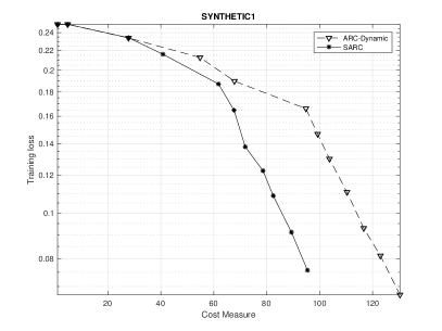
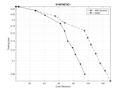
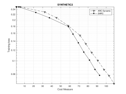
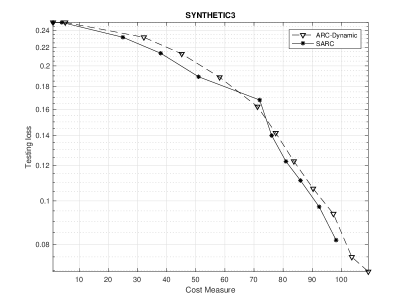
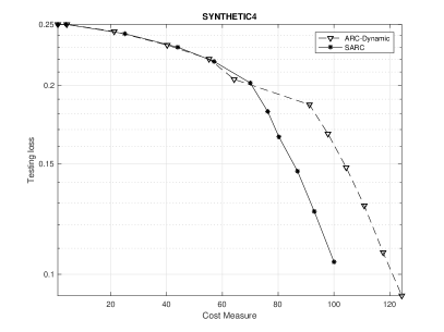
Figure 1: Synthetic datasets. Comparison of SARC (continuous line with asteriks) and ARC-Dynamic (dashed line with triangles) against the considered cost measure CM. Each row corresponds to a different synthetic dataset. Training loss (left) and testing loss (right) against CM with logarithmic scale on the $y$ axis.

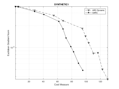
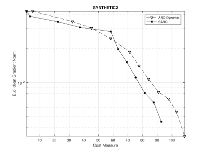
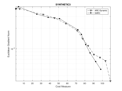
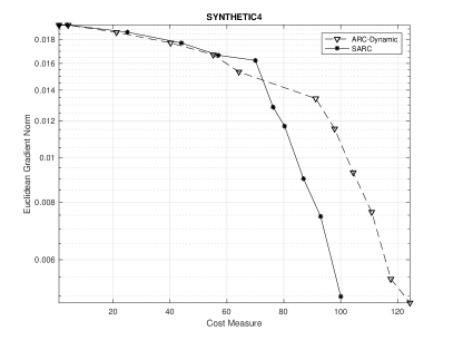
Figure 2: Synthetic datasets. Euclidean norm of the gradient against CM (training set) with logarithmic scale on the $y$ axis. SARC (continuous line with asteriks), ARC-Dynamic (dashed line with triangles).

In all cases, Figure 1 shows the savings gained by $SARC$ in terms of the overall computational cost, as well as the improvements in the training phase and the testing accuracy under the same cost measure. More in general, we stress that second order methods show their strength on these ill-conditioned datasets since all the tested procedures manage to reduce the norm of the gradient and reach high accuracies in the classification rate. Even if we believe that reporting binary classifications accuracy obtained by each of the considered methods at termination is relevant in itself, we remark that the higher accuracy obtained at termination by ARC-Dynamic (see Table 4) is just due to the fact the $SARC$ stops earlier. This should not be confused with a better performance of ARC-Dynamic, since Figure 1 highlights that, along all datasets, when $SARC$ stops its testing loss is sensibly below the corresponding one performed by ARC-Dynamic at the same CMT value.

In Figure 3, we finally analyse the adaptive choices of the sample sizes $\mathcal{D}_{j,k}$, $j\in\{1,2\}$, in (4.56). As expected, the two strategies are more or less comparable when selecting the sample sizes for Hessian approximations, while the number of samples used to compute gradient approximations by $SARC$ oscillates across all iterations, always remaining far below the full sample size. In so doing, we outline that too small values of $\tau_{0}$ seem to have a bad influence on the performance of $SARC$, while as $\tau_{0}$ increases it generally produces frequent saving in the CMT, once that it is above a certain threshold value. In support of this observation, we report in Figure 4 the variation of CMT against $\tau_{0}$ on Synthetic1 and Synthetic4. We finally notice that, except for a few iterations at the first stage of the iterative process, the sample size for Hessian approximation is lower than that used for gradient approximation. This is in line with the theory as the gradient is eventually required to be more accurate than the Hessian. In fact, the error in gradient approximation has to be of the order of $\|s_{k}\|^{2}$, while that in Hessian approximation has to be of the order of $\|s_{k}\|$, see Lemma 3.1 and 3.2.

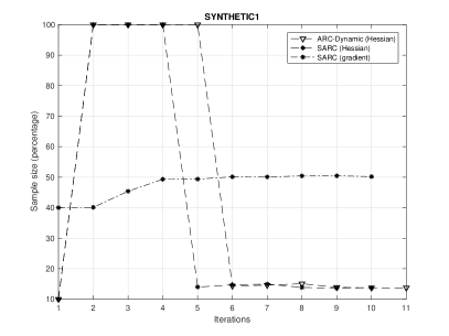
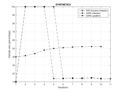
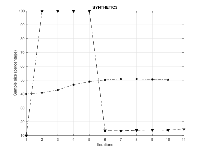
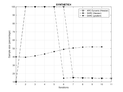
Figure 3: Synthetic datasets. Sample size for Hessian approximations employed by ARC-Dynamic (dashed line with triangles) and $SARC$ (dashed line with asteriks), together with the sample size for gradient approximations considered by $SARC$ (dotted dashed line with asteriks) against iterations.

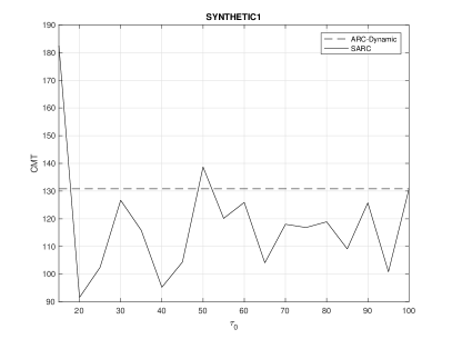
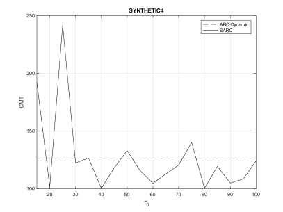
Figure 4: Cost Measure at Termination (CMT) against $\tau_{0}$ among $SARC$ (continuous line) and ARC-Dynamic (dashed line) on Synthetic1 and Synthetic4.

6 Conclusion and perspectives

We have proposed the stochastic analysis of the process generated by an ARC algorithm for solving unconstrained, nonconvex, optimisation problems under inexact derivatives information. The algorithm is an extension of the one in [3], since it employs approximated evaluations of the gradient with the main feature of mantaining the dynamic rule for building Hessian approximations, introduced and numerically tested in [3]. This kind of accuracy requirement is always reliable and computable when an approximation of the exact Hessian is needed by the scheme and, in contrast to other strategies such that the one in [18], does not require the inclusion of additional inner loops to be satisfied. With respect to the framework in [3], where in the finite-sum setting optimal complexity is restored with high probability, we have here provided properties of the method when the adaptive accuracy requirements of the derivatives involved in the model definition are not accomplished, with a view to search for the number of expected steps that the process takes to reach the prescribed accuracy level. The stochastic analysis is thus performed exploiting the theoretical framework given in [18], showing that the expected complexity bound matches the worst-case optimal complexity of the ARC framework. The possible lack of accuracy of the model has just the effect of scaling the optimal complexity we would derive from the deterministic analysis of the framework (see, e.g., [3, Theorem 4.2]), by a factor which depends on the probability $p$ of the model being sufficiently accurate. Numerical results confirm the theoretical achievements and highlight the improvements of the novel strategy on the computational cost in most of the tests with no worsening of the binary classification accuracy. This paper does not cover the case of noisy functions ([28, 20, 22]), as well as the second-order complexity analysis. The stochastic second-order complexity analysis of ARC methods with derivatives and function estimates will be a challenging line of investigation for future work. Concerning the latter point, we remark that a recent advance in [10], based on properties of supermartingales, has tackled with the second-order convergence rate analysis of a stochastic trust-region method. Funding: the authors are member of the INdAM Research Group GNCS and partially supported by INdAM-GNCS through Progetti di Ricerca 2019.

Acknowledgements. The authors dedicate this paper, in honor of his 70th birthday, to Alfredo Iusem. Thanks are due to Coralia Cartis, Benedetta Morini and Philippe Toint for fruitful discussion on stochastic complexity analysis and to two anonymous referees whose comments significantly improved the presentation of this paper.

References

• [1] A. Bandeira, K. Scheinberg, L. Vicente. Convergence of Trust-Region Methods Based on Probabilistic Models. SIAM Journal on Optimization 24(3), 1238–1264, 2014.
• [2] J. Barzilai, J. M. Borwein. Two-Point Step Size Gradient Methods. IMA Journal of Numerical Analysis 8, 14–148, 1998.
• [3] S. Bellavia, G.  Gurioli, B.  Morini. Adaptive Cubic Regularization Methods with Dynamic Inexact Hessian Information and Applications to Finite-Sum Minimization. IMA Journal of Numerical Analysis, https://doi.org/10.1093/imanum/drz076, 2019.
• [4] S. Bellavia, G. Gurioli, B. Morini, Ph. L. Toint. Adaptive Regularization Algorithms with Inexact Evaluations for Nonconvex Optimization. SIAM Journal on Optimization 29(4), 2281–2915, 2019.
• [5] A.S. Berahas, R. Bollapragada, J. Nocedal. An investigation of Newton-sketch and subsampled Newton methods. Optimization Methods and Software, 35, 661–680, 2020.
• [6] T. Bianconcini, G. Liuzzi, B. Morini, M. Sciandrone. On the use of iterative methods in cubic regularization for unconstrained optimization. Computational Optimization and Applications 60, 35–57, 2015.
• [7] E. G. Birgin, J. L. Gardenghi, J. M. Martínez, S. A. Santos, Ph. L. Toint. Worst-case evaluation complexity for unconstrained nonlinear optimization using high-order regularized models. Mathematical Programming, Ser. A, 163(1-2), 359-368, 2017.
• [8] E. G. Birgin, N. Krejić, J. M. Martínez. Iteration and evaluation complexity for the minimization of functions whose computation is intrinsically inexact. Mathematics of Computation 89 (321), 253–278, 2020.
• [9] Y. Carmon, J.C. Duchi, O. Hinder, A. Sidford. Lower bounds for finding stationary points I. Mathematical Programming, Series A, 1-50, 2019.
• [10] J. Blanchet, C. Cartis, M. Menickelly, K. Scheinberg. Convergence Rate Analysis of a Stochastic Trust-Region Method via Supermartingales. INFORMS Journal on Optimization 1(2), 92–119, 2019.
• [11] L. Bottou, F. E. Curtis, J. Nocedal. Optimization Methods for Large-Scale Machine Learning. SIAM Review 60(2), 223-311, 2018.
• [12] C. Cartis, N. I. M. Gould, Ph. L. Toint. Complexity bounds for second-order optimality in unconstrained optimization. Journal of Complexity 28(1), 93–108, 2012.
• [13] C. Cartis, N. I. M. Gould, Ph. L. Toint. On the oracle complexity of first-order and derivative-free algorithms for smooth nonconvex minimization SIAM Journal on Optimization 22(1), 66–86, 2012.
• [14] C. Cartis, N. I. M. Gould, Ph. L. Toint. An adaptive cubic regularisation algorithm for nonconvex optimization with convex constraints and its function-evaluation complexity. IMA Journal of Numerical Analysis 32(4), 1662–1695, 2012.
• [15] C. Cartis, N. I. M. Gould, Ph. L. Toint. Adaptive cubic overestimation methods for unconstrained optimization. Part I: motivation, convergence and numerical results. Mathematical Programming, Ser. A, 127, 245–295, 2011.
• [16] C. Cartis, N. I. M. Gould, Ph. L. Toint. Adaptive cubic overestimation methods for unconstrained optimization. Part II: worst-case function and derivative-evaluation complexity. Mathematical Programming, Ser. A, 130(2), 295–319, 2011.
• [17] C. Cartis, N. I. M. Gould, Ph. L. Toint. On the complexity of steepest descent, Newton’s and regularized Newton’s method for nonconvex unconstrained optimization. SIAM Journal on Optimization 20(6), 2833–2852, 2010.
• [18] C. Cartis, K. Scheinberg. Global convergence rate analysis of unconstrained optimization methods based on probabilistic models. Mathematical Programming, Ser. A, 159(2), 337–375, 2018.
• [19] K. H. Chang, M. K. Li, H. Wan. Stochastic Trust-Region Response-Surface Method (STRONG) – A New Response-Surface Framework for Simulation Optimization. INFORMS Journal on Computing 25(2), 193–393, 2013.
• [20] R. Chen. Stochastic Derivative-Free Optimization of Noisy Functions. Theses and Dissertations 2548, 2015.
• [21] X. Chen, B. Jiang, T. Lin, S. Zhang. On Adaptive Cubic Regularized Newton’s Methods for Convex Optimization via Random Sampling, arXiv:1802.05426, 2019.
• [22] R. Chen, M. Menickelly, K. Scheinberg. Stochastic optimization using a trust-region method and random models. Mathematical Programming 169(2), 447–487, 2018.
• [23] S. Gratton, C. W. Royer, L. N. Vicente, Z. Zhang. Complexity and global rates of trust-region methods based on probabilistic models. IMA Journal of Numerical Analysis 38(3), 1579–1597, 2018.
• [24] S. Gratton, C. W. Royer, L. N. Vicente, Z. Zhang. Direct Search Based on Probabilistic Descent. SIAM Journal on Optimization 25(3), 1515–1541, 2015.
• [25] J. M. Kohler, A. Lucchi. Sub-sampled cubic regularization for non-convex optimization. Proceedings of the 34th International Conference on Machine Learning 70, 1895–1904, 2017.
• [26] Y. Nesterov, B.T. Polyak. Cubic regularization of Newton method and its global performance. Mathematical Programming, Ser. A, 108, 177–205, 2006.
• [27] Y. Nesterov, V. Spokoiny. Random Gradient-Free Minimization of Convex Functions. Foundations of Computational Mathematics 17(2), 527–566, 2017.
• [28] C. Paquette, K. Scheinberg. A Stochastic Line Search Method with Expected Complexity Analysis. SIAM Journal on Optimization 30(1), 349–376, 2020.
• [29] S. Shashaani, F. S. Hashemi, R. Pasupathy. ASTRO-DF: A Class of Adaptive Sampling Trust-Region Algorithms for Derivative-Free Simulation Optimization. SIAM Journal on Optimization 28(4), 3145–3176, 2018.
• [30] J. Tropp. An Introduction to Matrix Concentration Inequalities. Foundations and Trends in Machine Learning 8(1-2), 1–230, 2015.
• [31] Z. Wang, Y. Zhou, Y. Liang, G. Lan. A note on inexact gradient and Hessian conditions for cubic regularized Newton’s method. Operations Research Letters 47, 146–149, 2019.
• [32] P. Xu, F. Roosta-Khorasani, M. W. Mahoney. Newton-type methods for non-convex optimization under inexact Hessian information. Mathematical Programming, https://doi.org/10.1007/s10107-019-01405-z, 2019.
• [33] P. Xu, F. Roosta-Khorasani, M. W. Mahoney. Second-Order Optimization for Non-Convex Machine Learning: An Empirical Study. Proceedings of the 2020 SIAM International Conference on Data Mining, 2020.
• [34] Z. Yao, P. Xu, F. Roosta-Khorasani, M. W. Mahoney. Inexact Non-Convex Newton-type Methods, arXiv:1802.06925, 2018.
• [35] D. Zhou, P. Xu, Q. Gu. Stochastic Variance-Reduced Cubic Regularization Methods. Journal of Machine Learning Research 20, 1–47, 2019.