From correlation functions to event shapes in QCD

Abstract

We present a method for calculating event shapes in QCD based on correlation functions of conserved currents. The method has been previously applied to the maximally supersymmetric Yang-Mills theory, but we demonstrate that supersymmetry is not essential. As a proof of concept, we consider the simplest example of a charge-charge correlation at one loop (leading order). We compute the correlation function of four electromagnetic currents and explain in detail the steps needed to extract the event shape from it. The result is compared to the standard amplitude calculation. The explicit four-point correlation function may also be of interest for the CFT community.

1 Introduction

Event shapes are important infrared safe observables in QCD Fox:1978vu ; Basham:1978bw ; Basham:1978zq ; Ellis:1980wv ; Kunszt:1989km ; Kunszt:1992tn ; Biebel:2001dm ; Belitsky:2001ij . For example, energy weighted cross sections can be used to measure the strong coupling constant, or to study jet physics. As such, they have the potential of connecting partonic and hadronic cross sections, especially within approaches that are valid non-perturbatively. One of the best known event shapes is the energy-energy correlation (EEC), widely studied in, e.g., $e^{+}e^{-}$ annihilation.

There has been considerable recent theoretical interest in event shapes. While numerical results are in principle enough for comparison with experiment, they may require heavy computer resources, or have intrinsic limitations as far as numerical accuracy is involved. Analytic results, on the other hand, are typically fast to evaluate to essentially arbitrary numerical precision.

To illustrate some of the recent analytic developments, let us mention that the next-to-leading-order (NLO) result for the EEC in QCD was obtained analytically in Dixon:2018qgp , 40 years after the leading-order (LO) result Basham:1978bw ; Basham:1978zq (the numerical result had been known earlier Kunszt:1992tn ; Glover:1994vz ). Remarkable progress was achieved in maximally supersymmetric Yang-Mills (${\cal N}=4$ sYM) theory, where the first ever NLO result was obtained in Belitsky:2013ofa . Moreover, while the EEC at NNLO is known only numerically in QCD DelDuca:2016ily , even an analytic NNLO result is available in the ${\cal N}=4$ sYM theory Henn:2019gkr . This progress was made possible by a novel approach Hofman:2008ar ; Belitsky:2013xxa ; Belitsky:2013bja that will also be central to this paper.

Furthermore, analytic approaches are much better suited to studying observables in extreme kinematic limits, such as the back-to-back limit or small angle limit, where large logarithms occur that need to be resummed in order to compare to experiment. Much recent progress has also been made in this direction, see Korchemsky:2019nzm ; Dixon:2019uzg ; Kologlu:2019mfz .

The traditional approach to computing event shapes uses amplitude methods and assembles the weighted cross sections from various ingredients, such as real and virtual contributions and phase-space integrals. While the final result is infrared finite, the intermediate expressions are infrared divergent and require intricate cancellations of singularities. The phase space integrals involved are often difficult to evaluate. In contrast, the novel approach is based on finite correlation functions. For example, in the case of the EEC, one starts with the correlation function of two currents representing the sources, and two energy-momentum tensors representing the detectors. The event shape is then obtained by sending the detectors to lightlike infinity and integrating over their working time. This is a conceptual improvement, as unnecessarily large intermediate expressions (involving unphysical regulated terms) are avoided.

Furthermore, this approach has the potential of exposing new structural properties of the observables: thanks to the connection between the two objects, the general properties of the four-point functions can inform us about the behavior of the event shapes, in particular beyond perturbation theory. For example, it was shown in Kologlu:2019mfz that the light-ray OPE gives a non-perturbative expansion for event shapes in terms of conformal blocks, and starting from OPE data they were able to make new four-loop predictions for the small angle expansion. Recently, a new integral representation for the EEC in the ${\cal N}=4$ sYM theory was found in Henn:2019gkr . It relates the EEC to a two-fold integral of the triple discontinuity of the four-point correlation function. In this way, information on the analytic properties of the correlation functions can be used to derive consequences for the event shapes.

In the literature, the correlation function approach was first proposed for energy and charge correlations in a generic conformal field theory in Hofman:2008ar . It was developed further in Belitsky:2013xxa and applied to these two event shapes (as well as to the mixed energy-charge correlation) in the particular framework of the ${\cal N}=4$ sYM theory in Belitsky:2013bja ; Belitsky:2013ofa . One should bear in mind that this theory is very special due to the extended super(conformal) symmetry, so one may doubt how useful the approach is in realistic QCD calculations. Moreover, supersymmetry relates different event shape observables, leaving no essential difference (a prefactor) between energy-energy and charge-charge correlations Belitsky:2013bja ; Belitsky:2014zha ; Korchemsky:2015ssa .

In this paper, we overcome these limitations. We work directly in QCD, and compute for the first time an event shape at one loop (or LO, i.e. order $O(g^{2})$ in the coupling) using the correlation function approach. Compared to other calculations, we observe that while supersymmetry has been helpful in the past and provided simplifications, it is not necessary for the method to work. Our main goal is the proof of a new concept, therefore we chose the simplest example of a charge-charge correlation (QQC). The method applies equally well to the EEC, although the computation of a correlation function with energy-momentum tensors is technically more involved.

This paper constitutes a first application of the new method to QCD, and therefore we also performed the calculation using standard amplitude methods, as a check. It should be emphasized that at the order we work in, the standard amplitude calculation is certainly more efficient. As we discuss in the outlook section, there are reasons to think that this will change at higher orders.

As a key ingredient of our analysis, we obtain the four-point correlation function of spin-one operators (electromagnetic currents) at one loop in QCD. This object is interesting in itself because the conserved currents are protected from UV renormalization. At the order $O(g^{2})$ the correlation function is conformally covariant because the beta function is of order $O(g^{3})$. Conformal four-point functions of operators of spin zero are well studied. They are very important in the context of the operator product expansion (OPE), and in particular for the conformal bootstrap. The general structure of conformal correlators of operators with spin has been discussed in, e.g., refs. Sotkov:1980qh ; Dymarsky:2013wla ; Kravchuk:2016qvl ; DK . As far as we are aware, our result is the first explicit loop-level non-supersymmetric example of such a four-point correlator. In principle, it could also be determined by the CFT data, i.e. the scaling dimensions and the structure constants, but this is yet to be worked out. We believe that our correlation function can serve as a first data point for OPE studies.

The paper is organized as follows. In Section 2 we review the definition of event shapes as weighted cross sections, and how they can be obtained from correlation functions. The following Section 3 is dedicated to the calculation of the correlation function of four currents at one loop in QCD using the Lagrangian insertion technique. The result for the four-point correlator, which may be of interest in itself to researchers in CFT, is given in eq. (3.25). In Section 4 we extract from this result the charge-charge correlation at LO in QCD, eq. (4.3), and we compare with the result of the traditional amplitude calculation, which can be found in Appendix B. Finally, we conclude and comment on future directions in Section 5.

2 Event shapes from correlation functions

In this section we review the basic definition of an event shape in QCD and its relationship to correlation functions. We restrict ourselves to the case of the electromagnetic current $J_{\mu}$ as the source and the associated electric charge ${\cal Q}$ as the detector. The generalization to other setups is straightforward Hofman:2008ar ; Belitsky:2013bja .

2.1 Event shapes as weighted cross sections

Let $P\cdot J(x)=P^{\mu}J_{\mu}(x)$ be a vector current $J_{\mu}(x)=\mbox{tr}\bar{\Psi}\gamma_{\mu}\Psi$ projected with a (complex) polarization vector $P^{\mu}$. Here $\Psi$ denotes a set of Dirac spinors describing the quarks and antiquarks in the fundamental representation of the color group. Further, let $|{X}\rangle$ be the final state created by this gauge invariant operator from the vacuum. To lowest order in the coupling it consists of a quark-antiquark pair. In general, the state $\int d^{4}xe^{iqx}P\cdot J(x)|{0}\rangle$ involves an arbitrary number of particles, with total momentum $q^{\mu}$ and zero color charge. The amplitude for the creation of a particular final state $|{X}\rangle$ with total momentum $k_{X}$ is

$$\langle{X|\int d^{4}xe^{iqx}P\cdot J(x)|0}\rangle=(2\pi)^{4}\delta^{(4)}(q-k_{X})\mathcal{M}_{J\to X}\,,$$ (2.1)

where

$$\mathcal{M}_{J\to X}=\langle{X|P\cdot J(0)|0}\rangle\,$$ (2.2)

is the form factor of the current on the on-shell state $X$. The total probability of this process is given by the sum over all the final states,

$$\sigma_{\rm tot}(q)=\sum_{X}(2\pi)^{4}\delta^{(4)}(q-k_{X})|\mathcal{M}_{J\to X}|^{2}\,.$$ (2.3)

Inserting the completeness relation

$$\sum_{X}|{X}\rangle\langle{X}|=1\,,$$ (2.4)

we can rewrite (2.3) as

$$\sigma_{\rm tot}(q) =\int d^{4}x\,e^{iqx}\langle{0|\bar{P}\cdot J(x)\ P\cdot J(0)|0}\rangle_{W}\,.$$ (2.5)

In other words, the total cross section can be interpreted as the Fourier transform of the two-point correlation function of the current, $\langle{J_{\mu}(x)J_{\nu}(0)}\rangle_{W}$, projected with the polarization matrix $\bar{P}^{\mu}P^{\nu}$. It is important to point out that this correlation function, defined in Minkowski space-time, is not time-ordered. This is denoted by the subscript $W$ meaning Wightman prescription. The alternative definition (2.5) of the total cross section (2.3) allows us to avoid infrared divergences at the intermediate steps and the necessity to sum over all the final states.

An event shape is defined as a weighted cross section with a weight factor $w(X)$ for the contribution of each state $|{X}\rangle$,

$$\sigma_{w}(q) =\sigma_{\rm tot}^{-1}\sum_{X}(2\pi)^{4}\delta^{(4)}(q-k_{X})w(X)|\mathcal{M}_{J\to X}|^{2}$$

$$=\sigma_{\rm tot}^{-1}\int d^{4}x\,e^{iqx}\sum_{X}\langle{0|\bar{P}\cdot J(x)|X}\rangle w(X)\langle{X|P\cdot J(0)|0}\rangle\,,$$ (2.6)

normalized so that $\sigma_{w}(q)=1$ for $w(X)=1$. The event shape $\sigma_{W}(q)$ describes the flow of the quantum numbers of the particles, i.e. energy, charges, etc. In this paper we study the case of charge flows.

For a given final state $|{X}\rangle=|{k_{1},\dots,k_{\ell}}\rangle$, consisting of $\ell$ massless particles, $k_{i}^{2}=0$, with charges $Q_{i}$ and total momentum $\sum_{i}k_{i}^{\mu}=q^{\mu}$, the weight factor is defined in the rest frame of the source $q^{\mu}=(q^{0},\vec{0})$ as

$$w_{\mathcal{Q}}(k_{1},\dots,k_{\ell})=\sum_{i=1}^{\ell}Q_{i}\,\delta^{(2)}(\Omega_{\vec{k}_{i}}-\Omega_{\vec{n}})\,,$$ (2.7)

where $k_{i}^{\mu}=(k_{i}^{0},\vec{k}_{i})$ and $\Omega_{\vec{k}_{i}}=\vec{k}_{i}/|\vec{k}_{i}|$ is the solid angle in the direction of $\vec{k}_{i}$. The unit vector $\vec{n}$ (with $\vec{n}^{2}=1$) indicates the direction of the charge flow. The weight (2.7) is the eigenvalue of the charge flow operator,

$$\mathcal{Q}(\vec{n})|{X}\rangle=w_{\mathcal{Q}}(X)|{X}\rangle\,.$$ (2.8)

The explicit expression for the operator $\mathcal{Q}(\vec{n})$ is given in terms of the time component of the current as an integral over the working time $t$ of the detector at the point $r\vec{n}$ infinitely far away from the collision point Ore:1979ry ; Sveshnikov:1995vi ; Korchemsky:1997sy ; Korchemsky:1999kt ; BelKorSte01 (see also Hofman:2008ar ) :

$$\mathcal{Q}(\vec{n})=\int_{0}^{\infty}dt\,\lim_{r\to\infty}r^{2}\,n^{i}\,J_{0}(t,r\vec{n})\,.$$ (2.9)

It satisfies the commutativity condition

$$[\mathcal{Q}(\vec{n}),\mathcal{Q}(\vec{n}^{\prime})]=0\qquad{\rm for}\ \vec{n}\neq\vec{n}^{\prime}\,,$$ (2.10)

meaning that the charge flows in the directions $\vec{n}$ and $\vec{n}^{\prime}$ can be measured separately.

Making use of (2.10) we can define a weight which measures the charge flows in two (or more) directions $\vec{n},\vec{n}^{\prime}$ simultaneously:

$$\mathcal{Q}(\vec{n})\mathcal{Q}(\vec{n}^{\prime})|{X}\rangle=w_{\mathcal{Q}(\vec{n})}(X)w_{\mathcal{Q}(\vec{n}^{\prime})}(X)|{X}\rangle\,.$$ (2.11)

Substituting eqs. (2.8) and (2.11) into (2.1) we can apply the completeness relation (2.4) and obtain the following representation of the corresponding weighted cross sections (or charge flow correlations)

$$\langle{\mathcal{Q}(\vec{n})}\rangle=\sigma_{\rm tot}^{-1}\int d^{4}x\,e^{iqx}\langle{0|\bar{P}\cdot J(x)\,\mathcal{Q}(\vec{n})\,P\cdot J(0)|0}\rangle_{W}\,,$$ (2.12)

$$\langle{\mathcal{Q}(\vec{n})\mathcal{Q}(\vec{n}^{\prime})}\rangle=\sigma_{\rm tot}^{-1}\int d^{4}x\,e^{iqx}\langle{0|\bar{P}\cdot J(x)\,\mathcal{Q}(\vec{n})\mathcal{Q}(\vec{n}^{\prime})\,P\cdot J(0)|0}\rangle_{W}\,,\quad\text{etc.}$$ (2.13)

We repeat that the product of operators in (2.12), (2.13) is not time ordered and their correlation functions are of the Wightman type. We will refer to the currents at points $x$ and $0$ as to the sink and source, respectively. The flow operators ${\cal Q}$ will be called detectors. The event shapes (2.12), (2.13), etc. are called single charge, charge-charge, etc. correlations.

In this paper we specialize to the lowest nontrivial perturbative level (LO), i.e. $O(g^{2})$. The standard calculation of the weighted cross section (2.13) from amplitudes is given in Appendix B. The bulk of the paper is devoted to obtaining the same result from the integrated correlation function of four electromagnetic currents.

2.2 Weighted cross sections from correlation functions

The underlying quantity in the definitions (2.12), (2.13), etc. of the weighted cross sections of $m$ charge flow detectors ${\cal Q}(\vec{n}_{1}),\ldots,{\cal Q}(\vec{n}_{m})$ are the Wightman correlation functions of $(m+2)$ currents $\langle{J_{\mu}(x)J_{\lambda_{1}}(x_{1})\ldots J_{\lambda_{m}}(x_{m})J_{\nu}(0)}\rangle_{W}$. In this subsection we explain how the Wightman correlation function in (2.12) can be obtained from its Euclidean counterpart by analytic continuation. We then apply it to computing the single-charge correlation at Born level (free theory). This simple example illustrates the procedure that we implement in the rest of the paper. At the end of the subsection we comment on the non-trivial analytic continuation of the four-point correlation function at loop level.

The Euclidean correlation functions have short-distance singularities when $x_{i}\to x_{j}$. In Minkowski space, additional singularities arise when the operators become lightlike separated, $x^{2}_{ij}\to 0$. In this case the analytic properties of the correlation function depend on the ordering of the operators.

In (2.9) we defined the charge flow operator in the rest frame of the source $q^{\mu}=(q^{0},\vec{0})$. The detector coordinates $x^{\mu}=(t,r\vec{n})$ can be decomposed in the basis of two lightlike vectors,

$$x^{\mu}=x_{+}n^{\mu}+x_{-}\bar{n}^{\mu}\,,\qquad n^{\mu}=(1,\vec{n})\,,\qquad\bar{n}^{\mu}=(1,-\vec{n})\,.$$ (2.14)

Manifest Lorentz covariance is restored by independent rescaling of these vectors,

$$n^{\mu}\to\rho\,n^{\mu}\,,\qquad\bar{n}^{\mu}\to\bar{\rho}\,\bar{n}^{\mu}\,,\qquad\rho,\bar{\rho}>0\,.$$ (2.15)

Then the covariant definition of the light-cone coordinates in (2.14) becomes

$$x_{+}={(x\bar{n})\over(n\bar{n})}\,,\qquad x_{-}={(xn)\over(n\bar{n})}\,.$$ (2.16)

We can now reformulate the detector limit $r\to\infty$ and the integration over the working time interval $0\leq t<\infty$ in terms of the light-cone variables $x_{\pm}$ (for the detailed physical motivation see Hofman:2008ar ; Belitsky:2013xxa ; Belitsky:2013bja ),

$$\mathcal{Q}(n)=\int_{-\infty}^{\infty}dx_{-}(n\bar{n})\lim_{x_{+}\to\infty}x_{+}^{2}\,J_{+}(x_{+}n+x_{-}\bar{n})\,.$$ (2.17)

Here $J_{+}\equiv\bar{n}^{\mu}J_{\mu}(x)/(n\bar{n})$ is the covariant light-cone projection of the current. Lorentz covariance requires that the charge flow operator transforms homogeneously under the rescaling (2.15), ${\cal Q}\to\rho^{-2}{\cal Q}$. As we shall see later on, the dependence on the auxiliary vector $\bar{n}$ is redundant and it drops out of the final result for the event shape.

2.3 A simple example: single charge correlation

Here we present a very simple example which illustrates all the main steps in obtaining an event shape from a Euclidean correlation function of currents. Consider the three-point function of currents made from a single Dirac fermion in the free theory (Born) approximation. According to (2.12), the single charge correlation is given by

$$\langle{\mathcal{Q}(\vec{n})}\rangle =\sigma_{\rm tot}^{-1}\int d^{4}x\,e^{iqx_{1}}\int_{-\infty}^{\infty}dx_{2-}(n\bar{n})$$

$$\times\lim_{x_{2+}\to\infty}x_{2+}^{2}\,\langle{0|\bar{P}\cdot J^{(v)}(x_{1})\,\bar{n}\cdot J^{(a)}(x_{2+}n+x_{2-}\bar{n})\,P\cdot J^{(v)}(0)|0}\rangle_{W}\,.$$ (2.18)

Using the Feynman rules from Section 3 we can easily compute the Euclidean correlation function. We find (up to a normalization factor)

$$G_{E} =\langle{\bar{P}\cdot J^{(v)}(x_{1})\ \bar{n}\cdot J^{(a)}(x_{2})\ P\cdot J^{(v)}(0)}\rangle_{E}$$

$$\sim\frac{1}{(x_{12}^{2}x_{1}^{2}x_{2}^{2})^{2}}\Big{[}\mbox{tr}(\bar{P}\tilde{x}_{12}\bar{n}\tilde{x}_{2}P\tilde{x}_{1})+\mbox{tr}(\bar{P}\tilde{x}_{1}P\tilde{x}_{2}\bar{n}\tilde{x}_{21})\Big{]}\,.$$ (2.19)

We need to perform the analytic continuation to the Wightman function in Minkowski space. To this end we replace each Euclidean interval by a Minkowski one, with the prescription

$$x^{2}_{ij}\ \rightarrow\ x^{2}_{ij}-i\epsilon x^{0}_{ij}\quad\text{for}\ i<j\,.$$ (2.20)

The next step is to take the detector limit of the Wightman function. The detector coordinate is $x_{2}^{\mu}=x_{2+}n^{\mu}+x_{2-}\bar{n}^{\mu}$. Then, for $x_{2+}\to\infty$ we have

$$x^{2}_{12}-i\epsilon x_{12}^{0}\ \to\ 2x_{2+}(x_{2-}(n\bar{n})-(x_{1}n)+i\epsilon)\,,$$

$$x^{2}_{2}-i\epsilon x_{2}^{0}\ \to\ 2x_{2+}(x_{2-}(n\bar{n})-i\epsilon)\,,$$ (2.21)

and we find from (2.19)

$$\lim_{x_{2+}\to\infty}x^{2}_{2+}G_{W}\sim\frac{(n\bar{n})\,i\epsilon_{\mu\nu\lambda\rho}\bar{P}^{\mu}P^{\nu}n^{\lambda}x_{1}^{\rho}}{(x_{2-}(n\bar{n})-(x_{1}n)+i\epsilon)^{2}(x_{2-}(n\bar{n})-i\epsilon)^{2}(x^{2}_{1}-i\epsilon x^{0}_{1})^{2}}\,.$$ (2.22)

According to (2.3), we have to integrate this expression over the detector time (or light-cone coordinate) $x_{2-}$. In (2.22) we see two double poles in $x_{2-}$ located on the two sides of the real axis. Closing the integration contour in the upper half-plane, we get

$$\int_{-\infty}^{\infty}dx_{2-}(n\bar{n})\lim_{x_{2+}\to\infty}x^{2}_{2+}G_{W}\sim\frac{i\epsilon_{\mu\nu\lambda\rho}\bar{P}^{\mu}P^{\nu}n^{\lambda}x_{1}^{\rho}}{((x_{1}n)-i\epsilon)^{3}(x_{1}^{2}-i\epsilon x_{1}^{0})^{2}}\ .$$ (2.23)

As expected, the auxiliary lightlike vector $\bar{n}$ has dropped out, and the result is homogeneous of degree $(-2)$ under the rescaling of the vector $n$. The Levi-Civita tensor originates from the parity-odd three-point correlation function that we started with.

The last step is the Fourier integral in (2.3), computed with the help of the formula

$$\int\frac{d^{4}x\,e^{iqx}}{(x^{2}-i\epsilon x^{0})^{a+1}((nx)-i\epsilon)^{b+1}}=\frac{(4\pi)^{3}\,(i/2)^{2a+b+3}}{\Gamma(a+1)\Gamma(a+b+1)}\theta(q^{2})\theta(q^{0})\frac{(q^{2})^{a+b}}{(nq)^{b+1}}\,.$$ (2.24)

Due to the current conservation condition we can identify $P_{\mu}\to P_{\mu}+\lambda q_{\mu}$. This allows us to choose a polarization vector orthogonal to the momentum, $(Pq)=(\bar{P}q)=0$. The total cross section in (2.3) is the Fourier transform of the two-point function of the source,

$$\int d^{4}x\,\langle{\bar{P}\cdot JP\cdot J}\rangle\sim\theta(q^{2})\theta(q^{0})(\bar{P}P)q^{2}\,.$$ (2.25)

In the rest frame $q^{\mu}=(q^{0},\vec{0})$ we have $P^{\mu}=(0,\vec{p})$ and $(\bar{P}P)=-|\vec{p}|^{2}$. Finally, the event shape is given by the expression

$$\langle{\mathcal{Q}(\vec{n})}\rangle\sim\frac{i}{|\vec{p}|^{2}}\,\epsilon_{ijk}p^{*}_{i}p_{j}n_{k}\,,$$ (2.26)

which exists only for a complex polarization vector Hofman:2008ar .

This concludes our pedagogical example. In Sect. 4 we apply the same procedure to the four-point correlation function of electromagnetic currents in QCD.

2.4 Charge-charge correlation for $e^{+}e^{-}$ annihilation

Let us recall the physics of the collider experiment $e^{+}e^{-}\to\gamma^{*}(q)\to X$. A pair of leptons $e^{+},e^{-}$ annihilates into a virtual photon $\gamma*$ with off-shell momentum $q^{\mu}$, which in turn decays into a number of quarks and gluons (final state $X$). The matrix element squared for this process can be written in the factorized form

$$\sum_{X}|{\cal M}_{e^{+}e^{-}\to X}|^{2}=L_{\mu\nu}H^{\mu\nu}\,.$$ (2.27)

The (symmetric) hadronic matrix $H$ accounts for the non-trivial decays $\gamma^{*}\to X$. In the case of charge-charge correlations under consideration, the charge-weighted hadronic matrix is identified with the correlation function of two currents and two charge operators (2.17),

$$H_{\mu\nu}(q,n,n^{\prime})=\int d^{4}x\,e^{iqx}\langle{0|J_{\mu}(x)\,\mathcal{Q}(n)\mathcal{Q}(n^{\prime})\,J_{\nu}(0)|0}\rangle_{W}\,.$$ (2.28)

The leptonic matrix $L$ is made from two vertices $e^{+}e^{-}\to\gamma^{*}$. In the typical case of an unpolarized beam (i.e. summing over the polarizations of the incoming particles) it has the following simple form Ellis:1991qj :

$$L_{\mu\nu}\sim\ell^{+}_{\mu}\ell^{-}_{\nu}+\ell^{+}_{\nu}\ell^{-}_{\mu}-\ell^{+}\cdot\ell^{-}\eta_{\mu\nu}\,.$$ (2.29)

Here $\ell^{\pm}$ (with $(\ell^{\pm})^{2}=0$ and $\ell^{+}+\ell^{-}=q$) are the on-shell momenta of the two leptons. The current conservation conditions $q^{\mu}L_{\mu\nu}=q^{\mu}H_{\mu\nu}=0$ become $L_{0\nu}=H_{0\nu}=0$ in the center-of-mass frame $q^{\mu}=(q^{0},\vec{0})$. In it $\ell^{\pm}=(q^{0}/2,\pm\vec{\ell})$ where the vector $\vec{\ell}$ defines the direction of the beam. Then (2.27), (2.29) yield

$$\sum_{X}|{\cal M}_{e^{+}e^{-}\to X}|^{2}\sim\left[\frac{(q^{0})^{2}}{4}\delta_{ij}+\vec{\ell}^{2}\delta_{ij}+2\ell_{i}\ell_{j}\right]H^{ij}(q^{0},\vec{n},\vec{n}^{\prime})\,.$$ (2.30)

The term in the brackets contains the information about the beam direction, relative to the directions of two detectors $\vec{n},\vec{n}^{\prime}$ (see Fig. 1). In some of the early papers Basham:1978bw ; Basham:1978zq the energy-energy correlation (EEC) was defined as a function of these three directions. Nowadays one considers a simplified observable (see, e.g., Fox:1978vu ; Ellis:1980wv ), in which one integrates over the direction of the beam $\vec{\ell}$, or equivalently, over the orientation of the detector plane relative to the beam. Rotation symmetry then tells us that the right-hand side of (2.30) is reduced to the trace $H^{ii}$. The Lorentz covariant version of this averaging procedure is

$$\int d^{2}\Omega_{\ell}\,\sum_{X}|{\cal M}_{e^{+}e^{-}\to X}|^{2}\sim\eta_{\mu\nu}H^{\mu\nu}=\int d^{4}x\,e^{iqx}\langle{0|J^{\mu}(x)\,\mathcal{Q}(n)\mathcal{Q}(n^{\prime})\,J_{\mu}(0)|0}\rangle_{W}\,.$$ (2.31)

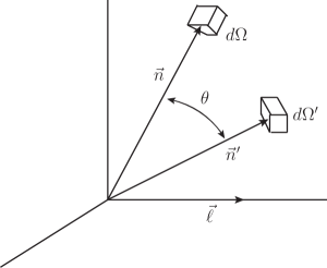
Figure 1: Two-detector configuration in $e^{+}e^{-}$ scattering. The vectors $\vec{n},\vec{n}^{\prime},\vec{\ell}$ denote the directions of the detectors and of the $e^{+}e^{-}$ beam, respectively.

In conclusion, the charge-charge correlation (2.13), averaged over the orientation of the detector plane, becomes

$$\langle{\mathcal{Q}(n)\mathcal{Q}(n^{\prime})}\rangle=\sigma_{\rm tot}^{-1}\int d^{4}x\,e^{iqx}\langle{0|J^{\mu}(x)\,\mathcal{Q}(n)\mathcal{Q}(n^{\prime})\,J_{\mu}(0)|0}\rangle_{W}\,.$$ (2.32)

This quantity depends on the virtual photon momentum $q$ and on the lightlike directions $n,n^{\prime}$ of the two detectors. Counting the dimensions of the operators involved in (2.32) and taking into account the scaling properties under (2.15), we conclude that

$$\langle{\mathcal{Q}(n)\mathcal{Q}(n^{\prime})}\rangle=\frac{F_{QQC}(\zeta)}{4\pi^{2}(nn^{\prime})^{2}}\,\,,\qquad\zeta=\frac{q^{2}(nn^{\prime})}{2(qn)(qn^{\prime})}\,.$$ (2.33)

In the center-of-mass frame the variable $\zeta$ is related to the angle between the two detectors,

$$2\zeta=(nn^{\prime})=1-\vec{n}\cdot\vec{n}^{\prime}\equiv 1-\cos\theta\,.$$ (2.34)

The purpose of the rest of the paper is to compute the event shape function $F_{QQC}(\zeta)$ at the leading order $O(g^{2})$ in massless QCD.

Before we move on, a comment is due on the analytic continuation of the four-point function in (2.32). At loop level the Euclidean correlator involves a non-trivial function with branch cuts (see (3.20) below). Its analytic continuation may seem to be a highly nontrivial task. A solution was found in Belitsky:2013xxa ; Belitsky:2013bja (following an idea of G. Mack Mack:2009mi ). It makes use of the Mellin representation of the function (3.20). Under the sign of the Mellin integral the analytic continuation is straightforward, according to the rule (2.20). We implement this procedure in Sect. 4.2.1. An alternative, even more efficient way is to replace the detector time integrations by the double discontinuity of the function (3.20) Caron-Huot:2017vep ; Alday:2017vkk ; Henn:2019gkr . This method is applied in Sect. 4.2.2.

3 Correlation function of four vector currents at one loop

In this section we calculate the four-point correlation function of electromagnetic currents in a massless gauge theory in the one-loop approximation. At this perturbative level non-abelian effects play no role, so our calculation is valid in QED as well as in QCD. The difference is only in the overall color factor.

The QCD Lagrangian contains gauge bosons (gluons) and fermions (quarks):

$$L=-\frac{1}{2}\mbox{tr}\,F_{\mu\nu}F^{\mu\nu}+\bar{\Psi}i\gamma^{\mu}{\cal D}_{\mu}\Psi\,.$$ (3.1)

Here ${\cal D}_{\mu}=\partial_{\mu}-igA_{\mu}$ is the covariant derivative with the gauge connection $A_{\mu}=A^{a}_{\mu}T_{a}$; $F_{\mu\nu}=\frac{i}{g}[{\cal D}_{\mu},{\cal D}_{\nu}]$ is the field-strength tensor; $\Psi$ is a Dirac spinor in the fundamental representation of the color group; the color generators of $SU(N_{c})$ are normalized as $\mbox{tr}(T_{a}T_{b})=\frac{1}{2}\delta_{ab}$.

The vector $J^{(v)}_{\mu}=\bar{\Psi}\gamma_{\mu}\Psi$ and axial vector $J^{(a)}_{\mu}=\bar{\Psi}\gamma_{\mu}\gamma_{5}\Psi$ currents are classically conserved and are associated with Noether charges. The conservation of the vector current $J^{(v)}_{\mu}$ takes place in the quantum theory as well. The corresponding composite operator is protected from infinite UV renormalization in perturbation theory. The conservation of the axial current at the quantum level is spoiled by the Adler-Bardeen anomaly.

The perturbative calculations in the gauge theory (3.1) usually require UV renormalization of the fields and coupling constant. However, in the one-loop approximation $O(g^{2})$ we can avoid these complications. Indeed, the interaction vertex renormalization effects play no role since $\beta(g)={O}(g^{3})$. Also, in our scheme the fermion propagator renormalization is finite at the one-loop level (see (3.22) below). Thus the correlation function of currents in the one-loop approximation

$$\langle{J_{\mu}(x_{1})\ldots J_{\nu}(x_{n})}\rangle=G^{\text{tree}}_{\mu\ldots\nu}(x_{1},\ldots,x_{n})+g^{2}\,G^{\text{1-loop}}_{\mu\ldots\nu}(x_{1},\ldots,x_{n})+O(g^{4})$$ (3.2)

is a finite four-dimensional quantity which does not require UV regularization. This is crucial for maintaining the conformal invariance of the classical Lagrangian at this perturbative level. As we show below, conformal invariance greatly facilitates our task.

In the following we use the two-component Lorentz spinor index notation, see Appendix A. We split the Dirac fermion in a pair of Weyl (or equivalently Majorana) fermions $\chi$ and $\psi$,

$$\Psi=(\chi_{\alpha}\,,\,\bar{\psi}^{{\dot{\alpha}}})\;\;\;,\;\;\;\;\;\;\bar{\Psi}=(\psi^{\alpha}\,,\,\bar{\chi}_{{\dot{\alpha}}})\,.$$ (3.3)

Then the Lagrangian (3.1) in the two-component notation takes the following form

$$L=L_{\rm YM}+i\psi^{\alpha}{\cal D}^{+}_{\alpha{\dot{\alpha}}}\bar{\psi}^{{\dot{\alpha}}}+i\chi^{\alpha}{\cal D}_{\alpha{\dot{\alpha}}}^{-}\bar{\chi}^{{\dot{\alpha}}}\,,\quad L_{\rm YM}\equiv-\frac{1}{2}\mbox{tr}\,F_{\mu\nu}F^{\mu\nu}\,,$$ (3.4)

where ${\cal D}^{\pm}_{\alpha{\dot{\alpha}}}=\sigma^{\mu}_{\alpha{\dot{\alpha}}}{\cal D}^{\pm}_{\mu}=\partial_{\alpha{\dot{\alpha}}}\mp igA_{\alpha{\dot{\alpha}}}$, so that the Weyl fermions $\psi$ and $\chi$ have opposite charges. The vector and axial vector currents

$$J^{(v)}_{\mu}=\psi^{\alpha}\sigma^{\mu}_{\alpha{\dot{\alpha}}}\bar{\psi}^{{\dot{\alpha}}}-\chi^{\alpha}\sigma^{\mu}_{\alpha{\dot{\alpha}}}\bar{\chi}^{{\dot{\alpha}}}\,,\qquad J^{(a)}_{\mu}=\psi^{\alpha}\sigma^{\mu}_{\alpha{\dot{\alpha}}}\bar{\psi}^{{\dot{\alpha}}}+\chi^{\alpha}\sigma^{\mu}_{\alpha{\dot{\alpha}}}\bar{\chi}^{{\dot{\alpha}}}$$ (3.5)

are independent linear combinations of the two Weyl currents. In the following we consider correlation functions of the currents $J_{\alpha{\dot{\alpha}}}\equiv\frac{1}{2}\sigma^{\mu}_{\alpha{\dot{\alpha}}}J_{\mu}=\psi_{\alpha}\bar{\psi}_{{\dot{\alpha}}}$ built out of one of the Weyl fermions. Since neither the interaction vertices nor the propagators mix the two kinds of fermions, we can immediately infer the correlation functions involving $J^{(v)}$ and/or $J^{(a)}$.

3.1 Computation of the one-loop correlation function via the Lagrangian insertion procedure

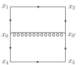
Figure 2: A typical Feynman graph of the correlator $\langle{JJJJ}\rangle$ at order $O(g^{2})$. It contains two interaction vertices corresponding to integrations $\int d^{4}x_{0}d^{4}x_{0^{\prime}}$.

The Feynman diagram calculations of correlation functions in coordinate space are quite different from the amplitude calculations in momentum space. In coordinate space we integrate over the space-time position of the interaction vertices. The typical Feynman graph depicted in Fig. 2 contributes to the four-point correlator of currents at order $O(g^{2})$. The integrations over $x_{0}$ and $x_{0^{\prime}}$ make this graph comparable to a two-loop amplitude Feynman graph. Fortunately, we can considerably simplify the task via the Lagrangian insertion method Eden:2000mv ; Eden:2010zz .

We start by rescaling the gauge field, $A_{\mu}\to\frac{1}{g}A_{\mu}$, after which the Lagrangian (3.1) takes the following form

$$L=\frac{1}{g^{2}}L_{\rm YM}+i\psi^{\alpha}{\cal D}^{+}_{\alpha{\dot{\alpha}}}\bar{\psi}^{{\dot{\alpha}}}+i\chi^{\alpha}{\cal D}^{-}_{\alpha{\dot{\alpha}}}\bar{\chi}^{{\dot{\alpha}}}\,,$$ (3.6)

where $L_{\rm YM}$ (3.4), the field strength $F$ and the covariant derivatives ${\cal D}$ do not depend on the coupling constant $g$. It is only present in (3.6) as an overall factor in front of $L_{\rm YM}$. We use the rescaled Lagrangian (3.6) in the path integral representation of the correlation function,

$$\langle{J_{\mu}(x_{1})\ldots J_{\nu}(x_{n})}\rangle=\int D\Phi\,e^{i\int d^{4}xL(x)}J_{\mu}(x_{1})\ldots J_{\nu}(x_{n})\,,$$ (3.7)

where $D\Phi$ denotes the integration measure for all the fields of the theory. Differentiating both sides of (3.7) with respect to $g^{2}$ we obtain

$$g^{2}\frac{\partial}{\partial g^{2}}\langle{J_{\mu}(x_{1})\ldots J_{\nu}(x_{n})}\rangle=-\frac{i}{g^{2}}\int D\Phi\,e^{i\int d^{4}xL(x)}\int d^{4}x\,L_{\rm YM}(x)J_{\mu}(x_{1})\ldots J_{\nu}(x_{n})$$

$$=-\frac{i}{g^{2}}\int d^{4}x\,\langle{L_{\rm YM}(x)J_{\mu}(x_{1})\ldots J_{\nu}(x_{n})}\rangle\,.$$ (3.8)

In this way we express the one-loop correction of the correlation function of currents (3.2) in terms of a correlator with one additional Lagrangian point, calculated at the lowest perturbative order (Born level),

$$g^{2}G^{\text{1-loop}}_{\mu\ldots\nu}(x_{1},\ldots,x_{n})=-i\int d^{4}x\,\langle{L_{\rm YM}(x)J_{\mu}(x_{1})\ldots J_{\nu}(x_{n})}\rangle_{\rm Born}\,.$$ (3.9)

The calculation of the $n-$point correlator of currents is done in two steps:

• Calculation of the $(n+1)-$point correlator with the operator $L_{\rm YM}$ at the insertion point at Born level,

  $$G_{\mu\ldots\nu}(x_{1},\ldots,x_{n}|x)=\langle{L_{\rm YM}(x)J_{\mu}(x_{1})\ldots J_{\nu}(x_{n})}\rangle_{\rm Born}\,.$$ (3.10)

  As we will see later on, this correlator is a rational function.

• Space-time integration over the Lagrangian insertion point,

  $$g^{2}G^{\text{1-loop}}_{\mu\ldots\nu}(x_{1},\ldots,x_{n})=-i\int d^{4}x\,G_{\mu\ldots\nu}(x_{1},\ldots,x_{n}|x)\,.$$ (3.11)

In the following subsections we proceed by successively implementing both tasks. As explained earlier, at this perturbative level the conformal symmetry of the Lagrangian (3.6) is preserved. Consequently, both the rational function in (3.10) and its integral in (3.11) enjoy manifest conformal covariance. This circumstance greatly facilitates the further steps in evaluating the charge-charge correlation.

3.2 Feynman diagrams at order $O(g^{2})$

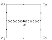
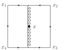
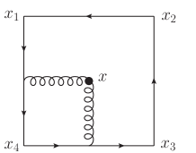
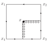
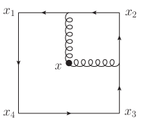
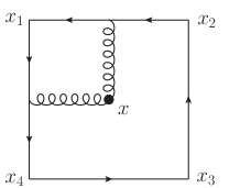
Figure 3: Feynman diagrams contributing to $\langle{L_{\rm YM}(x)J(x_{1})J(x_{2})J(x_{3})J(x_{4})}\rangle_{\rm Born}$ built out of fermion propagators and T-blocks shown in Fig. 5.A.

The tree-level correlator of currents $J_{\alpha{\dot{\alpha}}}=\psi_{\alpha}\bar{\psi}_{{\dot{\alpha}}}$ is a sum of products of fermion propagators. For example in the four-point case we obtain

$$\langle{J_{\alpha{\dot{\alpha}}}(x_{1})J_{\beta{\dot{\beta}}}(x_{2})J_{\gamma\dot{\gamma}}(x_{3})J_{\delta\dot{\delta}}(x_{4})}\rangle_{\text{tree}}=-\frac{N_{c}}{(2\pi^{2})^{4}}\sum_{\sigma\in S_{4}/\mathbb{Z}_{4}}\frac{(x_{\sigma_{1}\sigma_{2}})_{\alpha{\dot{\beta}}}(x_{\sigma_{2}\sigma_{3}})_{\beta\dot{\gamma}}(x_{\sigma_{3}\sigma_{4}})_{\gamma\dot{\delta}}(x_{\sigma_{4}\sigma_{1}})_{\delta\dot{\alpha}}}{x_{\sigma_{1}\sigma_{2}}^{4}x_{\sigma_{2}\sigma_{3}}^{4}x_{\sigma_{3}\sigma_{4}}^{4}x_{\sigma_{1}\sigma_{4}}^{4}}$$ (3.12)

where the sum over the inequivalent permutations amounts to Bose symmetrization. Here we tacitly imply permuting the Lorentz indices along with the points $x_{i}$. Expression (3.12) is manifestly conformal, carrying conformal weight $(+3)$ at each point.

Let us now consider the Born-level correlator of four currents with one Lagrangian insertion. The corresponding Feynman diagrams are shown in Figs. 3 and 4. We also need to Bose symmetrize them by adding five noncyclic permutations of the external points like at tree level. Each diagram contains two interaction vertices $g\psi A\bar{\psi}$ from the Lagrangian (3.4), so the Born-level correlator is of order $O(g^{2})$ in the coupling.

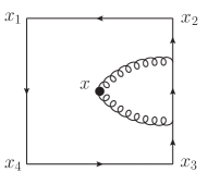
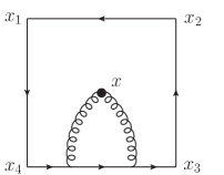
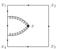
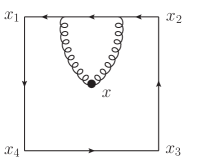
Figure 4: Feynman diagrams contributing to $\langle{L_{\rm YM}(x)J(x_{1})J(x_{2})J(x_{3})J(x_{4})}\rangle_{\rm Born}$ built out of fermion propagators and Lagrangian insertions of the type shown in Fig. 5.B.

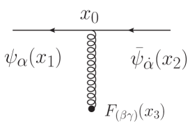
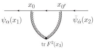
(A)		(B)

Figure 5: (A) T-block diagram (3.13) representing $\langle{\psi\bar{\psi}F}\rangle$ at Born level. (B) Lagrangian insertion in the fermion propagator (3.14).

Inspecting the Feynman diagrams in Fig. 3 we see that they are products of fermion propagators and the so-called T-blocks – an interaction vertex of two fermions and a gluon with the field strength at the gluon propagator end, see Fig. 5.A,

$$\langle{\psi_{\alpha}(x_{1})\bar{\psi}_{\dot{\alpha}}(x_{2})F_{a}^{\mu\nu}(x_{3})}\rangle_{g}=\frac{ig\,T_{a}}{(2\pi)^{6}}\int d^{4}x_{0}\,\partial_{\alpha}^{\dot{\beta}}\frac{1}{x_{10}^{2}}\partial^{\beta}_{{\dot{\alpha}}}\frac{1}{x_{20}^{2}}\sigma^{[\nu}_{\beta{\dot{\beta}}}\partial^{\mu]}\frac{1}{x_{30}^{2}}$$

$$=\frac{g\,T_{a}}{(2\pi)^{4}}\left\{\frac{4(x_{12})_{\alpha{\dot{\alpha}}}}{x^{4}_{12}}\frac{x_{31}^{[\mu}x_{32}^{\nu]}}{x^{2}_{13}x^{2}_{23}}-\frac{(x_{12}\tilde{x}_{23}\sigma^{[\mu}\tilde{\sigma}^{\nu]}x_{32})_{\alpha{\dot{\alpha}}}}{2x^{2}_{12}x^{2}_{13}x^{4}_{23}}-\frac{(\tilde{x}_{21}x_{13}\tilde{\sigma}^{[\mu}\sigma^{\nu]}\tilde{x}_{31})_{\alpha{\dot{\alpha}}}}{2x^{2}_{12}x^{4}_{13}x^{2}_{23}}\right\}\,.$$ (3.13)

The integration in eq. (3.13) is carried out by means of the star-triangle relation, which yields a rational function. This object is gauge covariant (not invariant), consequently it is not conformally covariant.

The diagrams in Fig. 4 contain another building block depicted in Fig. 5.B. It is a Born-level diagram representing the coupling of the Yang-Mills Lagrangian to the fermion propagator. This diagram contains two interaction vertices with integrations $\int d^{4}x_{0}d^{4}x_{0^{\prime}}$. Remarkably, it turns out to be a rational function,

$$\langle{\psi_{\alpha}(x_{1})\bar{\psi}_{\dot{\alpha}}(x_{2})\,\mbox{tr}\,(F_{\mu\nu}^{2})(x_{3})}\rangle_{g^{2}}$$

$$=\frac{2ig^{2}C_{F}}{(2\pi)^{10}}\int d^{4}x_{0}d^{4}x_{0^{\prime}}\partial_{\alpha{\dot{\beta}}}\frac{1}{x_{10}^{2}}\partial_{\beta\dot{\gamma}}\frac{1}{x_{00^{\prime}}^{2}}\partial_{\gamma{\dot{\alpha}}}\frac{1}{x_{20^{\prime}}^{2}}\left[2\epsilon^{\beta\gamma}\epsilon^{{\dot{\beta}}\dot{\gamma}}\partial_{\mu}\frac{1}{x_{30}^{2}}\partial^{\mu}\frac{1}{x_{30^{\prime}}^{2}}-\partial^{\dot{\gamma}\gamma}\frac{1}{x_{30}^{2}}\partial^{{\dot{\beta}}\beta}\frac{1}{x_{30^{\prime}}^{2}}\right]$$

$$=\frac{2ig^{2}C_{F}}{(2\pi)^{6}}\frac{(x_{12})_{\alpha{\dot{\alpha}}}}{x_{12}^{4}x_{13}^{4}x_{23}^{4}}[x_{12}^{4}+x_{13}^{4}+x_{23}^{4}-2x_{12}^{2}x_{13}^{2}-2x_{12}^{2}x_{23}^{2}-2x_{13}^{2}x_{23}^{2}]\,,$$ (3.14)

where

$$C_{F}=\frac{N_{c}^{2}-1}{2N_{c}}$$ (3.15)

is the Casimir invariant of the fundamental color representation of the fermions. Similarly to (3.13), expression (3.14) is not conformally covariant.

Combining all the ingredients above, we obtain a rather bulky expression for the $(4+1)$-point Born-level correlation function, which is the one-loop integrand of the correlator of four currents, see eq. (3.11). Let us emphasize once more that the integrand is a finite rational function living in four space-time dimensions. Despite of the fact that the individual Feynman graphs contributing to the integrand are not conformally covariant, the integrand itself (i.e. the gauge invariant sum of all the graphs) is conformal. We explicitly checked that this property holds.

$\begin{array}[]{c}\includegraphics[width=113.81102pt]{./figures/integrand4J_6_der.eps}\end{array}$

$\Longrightarrow$

$\begin{array}[]{c}\includegraphics[width=113.81102pt]{./figures/integrand4J_contr.eps}\end{array}$

$\Longleftarrow$

$\begin{array}[]{c}\includegraphics[width=113.81102pt]{./figures/integrand4J_9_der.eps}\end{array}$

Figure 6: The current conservation Ward identity (3.16) can be easily verified at the level of the correlator Feynman diagrams given in Figs. 3 and 4.

An additional check of our result for the integrand is provided by current conservation. The divergence of the correlator with respect to each current point must vanish (up to possible contact terms), e.g.

$$\partial^{{\dot{\alpha}}\alpha}_{1}\langle{L_{\rm YM}(x)\,J_{\alpha{\dot{\alpha}}}(x_{1})\ldots J_{\delta\dot{\delta}}(x_{4})}\rangle_{\rm Born}=0\,.$$ (3.16)

We checked that the integrand obtained has this property. The current conservation can be easily seen at the level of the Feynman graphs. Since by definition

$$\partial^{{\dot{\alpha}}\alpha}\langle{\psi_{\alpha}(x)\bar{\psi}_{{\dot{\beta}}}(0)}\rangle=\delta^{{\dot{\alpha}}}_{{\dot{\beta}}}\delta^{(4)}(x)\,,$$ (3.17)

the derivative shrinks the fermion propagator to a point, and the ‘shrunk’ Feynman diagrams cancel pairwise, as depicted in Fig. 6. Using eq. (3.17) we can derive first order differential equations for the building blocks (3.13) and (3.14). We checked that the provided rational expressions satisfy these differential equations.

3.3 Result for the four-point correlation function

Having obtained the one-loop integrand, at the next step we integrate over the Lagrangian insertion point, see eq. (3.11). Even though the correlator of four currents is UV finite in the one-loop approximation, the integration of some individual terms of the integrand could lead to UV divergences. So we need to introduce an intermediate regulator. We use dimensional regularization and integrate over the Lagrangian point in $D=4-2\epsilon$ dimensions. Since the integrand carries Lorentz spinor indices, we have to specify how to treat this objects in $D$ dimensions. We assume that the $\sigma$ matrices are four-dimensional and we do the spinor algebra in four space-time dimensions. When rewriting the integrand numerator we have the choice between two prescriptions: either $(x\tilde{x})_{\alpha}{}^{\beta}=\delta_{\alpha}^{\beta}x^{2}$ or $(x\tilde{x})_{\alpha}{}^{\beta}=\delta_{\alpha}^{\beta}(x^{2}-\mu^{2})$ where $x^{2}$ is $D$-dimensional and $\mu^{2}$ is the $(-2\epsilon)$-dimensional part of $x^{2}$ Bern:1995db . We did the calculations in both schemes and found identical results.

The integrals that we need can be mapped to the well-known families of one-loop amplitude integrals with massive legs and massless internal propagators. The numerators of the integrands are tensors of maximal rank two. We perform the tensor reduction procedure in coordinate space in order to reduce them to scalar one-loop integrals (see Appendix C). Then we do IBP reduction of the scalar integrals to a set of master integrals: bubble, three-mass triangle, and four-mass box integrals. Removing the regulator $\epsilon\to 0$ we find that the triangle integrals are suppressed, and all the $\epsilon$-poles in the individual terms cancel out in the sum. The logarithmic terms $\log(x_{ij}^{2})$ in the $\epsilon$-expansion of the bubble integrals combine together into logarithms of the conformal cross-ratios

$$u=\frac{x_{12}^{2}x_{34}^{2}}{x_{13}^{2}x_{24}^{2}}\;,\qquad v=\frac{x_{14}^{2}x_{23}^{2}}{x_{13}^{2}x_{24}^{2}}\;.$$ (3.18)

Thus the one-loop correlator takes the following form

$$G^{\text{1-loop}}(x_{1},\ldots,x_{4})$$

$$=-\frac{4N_{c}C_{F}}{(2\pi)^{10}}\left[R_{c}(x)\,\Phi^{(1)}(u,v)+R_{u}(x)\,\log(u)+R_{v}(x)\,\log(v)+R_{r}(x)\right]+R^{\prime}_{r}(x)\,,$$ (3.19)

where we omit the Lorentz indices. The various $R$’s are rational functions of the coordinates. They are conformally covariant tensors carrying spin 1 and weight $(+3)$ at each point. The function $\Phi^{(1)}$ is the well-known cross integral (four-mass box integral in the amplitude literature),

$$\Phi^{(1)}(u,v)=\frac{1}{\bar{z}-z}\left[2{\rm Li}_{2}\left(\frac{z}{z-1}\right)-2{\rm Li}_{2}\left(\frac{\bar{z}}{\bar{z}-1}\right)-\log\left(\frac{z\bar{z}}{(1-z)(1-\bar{z})}\right)\log\left(\frac{1-z}{1-\bar{z}}\right)\right]$$ (3.20)

given here in the $z,\bar{z}$ parametrization of the conformal cross-ratios

$$u=z\bar{z}\;,\qquad v=(1-z)(1-\bar{z})\,.$$ (3.21)

We remark that $\Phi^{(1)}$ is regular at $z=\bar{z}$. The rational term $R_{r}(x)$ in (3.19) comes from the $\epsilon\cdot\frac{1}{\epsilon}=1$ cancellations between the simple poles of the bubbles and the $D$-dependent coefficients of the IBP relations and the tensor reductions.

The conformal covariance of our final result (3.19) is a strong check of our calculation. Note however that the rational functions $R_{c},\,R_{u},\,R_{v},\,R_{r}$ do not arise in a manifestly conformal form in our Feynman graph calculation. To find a conformal representation for them we study their singularities, construct a conformal ansatz for their numerators, and match them with the ansatz. In the case of interest we need to list the conformal polynomial tensors of conformal weight $(-6)$ at each point. This is done as follows. We use the conformal expressions $(x_{ij})_{\alpha_{i}{\dot{\alpha}}_{j}}$, $(x_{ik}\tilde{x}_{kj})_{\alpha_{i}\alpha_{j}}$, and $(\tilde{x}_{ik}x_{kj})_{{\dot{\alpha}}_{i}{\dot{\alpha}}_{j}}$ as elementary constituents, and form products that are conformal tensors carrying the eight Lorentz spinor indices of the currents, $\alpha{\dot{\alpha}}\ldots\delta\dot{\delta}$. In this way we find 242 linearly independent over $\mathbb{Q}$ polynomial conformal tensors. Then we complement them with polynomials in $x_{ij}^{2}$ such that each tensor carries conformal weight $(-6)$ at each point, and we find that only 1024 of them are linearly independent over $\mathbb{Q}$. We take them as a basis of conformal structures for the numerators of $R_{c},\,R_{u},\,R_{v},\,R_{r}$.

The last rational term $R^{\prime}_{r}(x)$ in (3.19) stays apart. It comes from integrating out the Lagrangian insertion point in the Feynman diagrams in Fig. 4. Integrating the building block (3.14) we find the one-loop propagator correction

$$\int d^{4}x_{3}\,\langle{\psi_{\alpha}(x_{1})\bar{\psi}_{\dot{\alpha}}(x_{2})\,\mbox{tr}\,(F_{\mu\nu}^{2})(x_{3})}\rangle_{g^{2}}=-\frac{3g^{2}C_{F}}{(2\pi)^{4}}\frac{(x_{12})_{\alpha{\dot{\alpha}}}}{x_{12}^{4}}\,,$$ (3.22)

which is proportional to the free fermion propagator. Consequently, $R^{\prime}_{r}$ is proportional to the tree-level correlator (3.12),

$$R^{\prime}_{r}(x_{1},x_{2},x_{3},x_{4})=\frac{3g^{2}N_{c}C_{F}}{8(2\pi^{2})^{5}}\sum_{\sigma\in S_{4}/\mathbb{Z}_{4}}\frac{(x_{\sigma_{1}\sigma_{2}})_{\alpha{\dot{\beta}}}(x_{\sigma_{2}\sigma_{3}})_{\beta\dot{\gamma}}(x_{\sigma_{3}\sigma_{4}})_{\gamma\dot{\delta}}(x_{\sigma_{4}\sigma_{1}})_{\delta\dot{\alpha}}}{x_{\sigma_{1}\sigma_{2}}^{4}x_{\sigma_{2}\sigma_{3}}^{4}x_{\sigma_{3}\sigma_{4}}^{4}x_{\sigma_{1}\sigma_{4}}^{4}}\,.$$ (3.23)

Obviously, this term is conformal on its own and satisfies the current conservation.

Differentiating $\Phi^{(1)}$ with respect to the variables $u,v$ gives

$$\partial_{u}\Phi^{(1)}=\frac{1}{\lambda^{2}}\left[(1-u+v)\Phi^{(1)}+2\log u+\frac{1-u-v}{u}\log v\right],$$

$$\partial_{v}\Phi^{(1)}=\frac{1}{\lambda^{2}}\left[(1+u-v)\Phi^{(1)}+2\log v+\frac{1-u-v}{v}\log u\right],$$ (3.24)

where $\lambda^{2}(u,v)=1+u^{2}+v^{2}-2u-2v-2uv=(\bar{z}-z)^{2}$. Thus one sees that the current conservation Ward identity for (3.19) relies on a nontrivial system of differential equations relating the functions $R_{c},\,R_{u},\,R_{v},\,R_{r}$. We explicitly checked that (3.19) does satisfy current conservation with respect to each external point.

An essential drawback of the representation (3.19) of our result is that the rational functions $R_{c},\,R_{u},\,R_{v},\,R_{r}$ contain spurious poles at $z=\bar{z}$. We would like to obtain another representation for the correlator which has only the physical singularities determined by the OPE. By differentiating further eqs. (3.24) we obtain relations which allow us to express $\log(u)$, $\log(v)$, $\Phi^{(1)}$ in terms of the second-order derivatives $\partial^{2}_{uu}\Phi^{(1)}$, $\partial^{2}_{vv}\Phi^{(1)}$, $\partial^{2}_{uv}\Phi^{(1)}$. Substituting these expressions back in (3.19) we find that all the $(z-\bar{z})$ factors in the denominators of the rational coefficients disappear. The resulting expression contains only physical singularities. Finally, we assemble the $x_{ij}^{2}$ into conformal cross-ratios and the correlator takes the following form

$$G^{\text{1-loop}}(x_{1},\ldots,x_{4})= -\frac{4N_{c}C_{F}}{(2\pi)^{10}}\frac{1}{(x_{13}^{2}x_{24}^{2})^{4}}\biggl{[}\partial_{uu}^{2}\Phi^{(1)}\sum_{I}c_{uu}^{(I)}(u,v)T_{I}+\partial_{vv}^{2}\Phi^{(1)}\sum_{I}c_{vv}^{(I)}(u,v)T_{I}$$

$$+\partial_{uv}^{2}\Phi^{(1)}\sum_{I}c_{uv}^{(I)}(u,v)T_{I}+\sum_{I}c_{0}^{(I)}(u,v)T_{I}\biggr{]}+R^{\prime}_{r}\,.$$ (3.25)

The coefficients $c(u,v)$ are polynomial in $u,v,u^{-1},v^{-1}$. The Lorentz indices are carried by 31 conformal structures $\{T_{I}\}_{I=1}^{31}$ with conformal weight $(-1)$ at each point. We can write them down schematically in the following form

$$T_{I}=\sum_{J}(b^{(J)}_{0}+b^{(J)}_{u}u+b_{v}^{(J)}v)\,t_{J}\,,$$ (3.26)

where $b_{0},\,b_{u},\,b_{v}$ are integers and the tensors $t_{J}$ are formed from conformally covariant products of $(x_{ij})_{\alpha_{i}\dot{\alpha}_{j}}$, $(x_{ik}\tilde{x}_{kj})_{\alpha_{i}\alpha_{j}}$ and $(\tilde{x}_{ik}x_{kj})_{{\dot{\alpha}}_{i}{\dot{\alpha}}_{j}}$. The tensors $T_{I}$ are parity even and real in Minkowski kinematics, i.e. converting the spinor indices to vector indices,

$$(T_{I})_{\alpha{\dot{\alpha}}\ldots\delta\dot{\delta}}\;\tilde{\sigma}^{{\dot{\alpha}}\alpha}_{\mu}\,\tilde{\sigma}^{{\dot{\beta}}\beta}_{\nu}\tilde{\sigma}^{\dot{\gamma}\gamma}_{\lambda}\tilde{\sigma}^{\dot{\delta}\delta}_{\rho}\,,$$ (3.27)

we find that the resulting expressions do not involve the Levi-Civita tensor. The explicit expressions for $T_{I}$ and $c(u,v)$ are provided in the ancillary file. Of course, our choice of basis of conformal tensors in (3.25) is not unique. The main advantage of this choice is that the basis tensors and their coefficients do not have unphysical singularities.

We calculated the correlation function (3.25) of four currents $J_{\alpha{\dot{\alpha}}}=\psi_{\alpha}\bar{\psi}_{{\dot{\alpha}}}$ built from one Weyl spinor and its conjugate (or equivalently, from one Majorana fermion). One can easily see that the one-loop Feynman rules yield the same result for the correlator of four currents $\tilde{J}_{\alpha{\dot{\alpha}}}=\chi_{\alpha}\bar{\chi}_{{\dot{\alpha}}}$. Since the interactions do not mix the $\psi$ and $\chi$ fields, see (3.4), the connected components of the correlators involving a mixture of $J$ and $\tilde{J}$ have to vanish. We conclude that the correlator of four vector electromagnetic currents $J^{(v)}$ from (3.5) equals twice (3.25). If instead we use an odd number of axial currents from (3.5), the one-loop correlator vanishes.

4 From the correlation function to the charge-charge correlation

In this section we evaluate the event shape function (2.33) for the charge-charge correlation at one loop. We substitute our result (3.25) for the correlation function of four electromagnetic currents $J\equiv J^{(v)}$ in the definitions (2.32) and (2.17). The charge flow correlation between two detectors in the direction of $\vec{n}$ and $\vec{n}^{\prime}$ is given by

$$\langle{\mathcal{Q}(\vec{n})\mathcal{Q}(\vec{n}^{\prime})}\rangle=\sigma_{\text{tot}}^{-1}\int d^{4}x_{14}e^{iqx_{14}}\int_{-\infty}^{\infty}dx_{2-}dx_{3-}$$ (4.1)

$$\lim_{x_{2+},x_{3+}\rightarrow\infty}x_{2+}^{2}x_{3+}^{2}\langle{J_{\alpha{\dot{\alpha}}}(x_{1})\,J_{\beta{\dot{\beta}}}(x_{2})\,J_{\gamma{\dot{\gamma}}}(x_{3})\,J_{\delta{\dot{\delta}}}(x_{4})}\rangle\,\epsilon^{\alpha\delta}\epsilon^{{\dot{\alpha}}\dot{\delta}}\,\bar{n}^{{\dot{\beta}}\beta}\bar{n}^{\prime{\dot{\gamma}}\gamma}\,.$$

As explained in Sect. 2.4, we consider a rotationally invariant event shape, which allows us to contract the Lorentz indices at points 1 and 4.

4.1 Detector limit

In (4.1) the two detectors at points 2 and 3 are infinitely far away from the sink and source at points 1 and 4. In order to take the detector limit, we introduce the light-cone parametrization (2.14) of the detectors,

$$x_{2}^{\mu}=x_{2+}\,n^{\mu}+x_{2-}\,\bar{n}^{\mu}\;,\qquad x_{3}^{\mu}=x_{3+}\,n^{\prime\mu}+x_{3-}\,\bar{n}^{\prime\mu}\,,$$ (4.2)

in the basis of the lightlike vectors $n^{2}=\bar{n}^{2}=(n^{\prime})^{2}=(\bar{n}^{\prime})^{2}=0$. The detector currents are projected, $J_{+}(x_{2})=\bar{n}^{\mu}J_{\mu}(x_{2})$ and $J_{+}(x_{3})=\bar{n}^{\prime\mu}J_{\mu}(x_{3})$. Sending the detectors to infinity amounts to the limit $x_{2+},x_{3+}\to\infty$ in which

$$x_{12}^{2}\rightarrow\,2x_{2+}x_{21-},\;\;x_{13}^{2}\rightarrow\,2x_{3+}x_{31-},\;\;x_{24}^{2}\rightarrow\,2x_{2+}x_{24-},\;\;x_{34}^{2}\rightarrow\,2x_{3+}x_{34-},$$

$$x_{14}^{2}\rightarrow x_{14}^{2},\;\;x_{23}^{2}\rightarrow-2(nn^{\prime})x_{2+}x_{3+}\,.$$ (4.3)

Here we use the short-hand notations

$$x_{21-}=x_{2-}(n\bar{n})-(nx_{1})\;,\;x_{24-}=x_{2-}(n\bar{n})-(nx_{4})\;,$$

$$x_{31-}=x_{3-}(n^{\prime}\bar{n}^{\prime})-(n^{\prime}x_{1})\;,\;x_{34-}=x_{3-}(n^{\prime}\bar{n}^{\prime})-(n^{\prime}x_{4})\,.$$ (4.4)

We find that the detector limit takes the following form

$$\lim_{x_{2+},x_{3+}\rightarrow\infty}x_{2+}^{2}x_{3+}^{2}\,\langle{J^{\mu}(x_{1})J_{+}(x_{2})J_{+}(x_{3})J_{\mu}(x_{4})}\rangle=-\frac{g^{2}N_{c}C_{F}}{2^{4}\pi^{10}}\frac{(n\bar{n})(n^{\prime}\bar{n}^{\prime})}{x_{14}^{8}\,(nn^{\prime})^{3}}\,\mathcal{G}(u,v,\gamma)\,,$$ (4.5)

where (see (3.18))

$$u=\frac{x_{21-}x_{34-}}{x_{31-}x_{24-}}\;,\quad v=-\frac{x_{14}^{2}(nn^{\prime})}{2x_{31-}x_{24-}}\;,\quad\gamma=\frac{2(nx_{14})(n^{\prime}x_{14})}{x_{14}^{2}\,(nn^{\prime})}\,.$$ (4.6)

The dimensionless and inert under the rescalings (2.15) variable $\gamma$ is the space-time counterpart of the angular variable $\zeta$ in (2.33). The function $\mathcal{G}(u,v,\gamma)$ is given by

$$\mathcal{G}(u,v,\gamma)={\cal P}(u,v,\gamma)\,\Phi^{(1)}(u,v)+\frac{v^{2}}{u^{3}}r_{r}(u,v,\gamma)\,,$$ (4.7)

where ${\cal P}$ is a second-order differential operator,

$${\cal P}(u,v,\gamma)\equiv\frac{v^{4}}{u^{2}}\left[r_{uu}(u,v,\gamma)\,\partial_{uu}^{2}+r_{uv}(u,v,\gamma)\,\partial_{uv}^{2}+r_{vv}(u,v,\gamma)\,\partial_{vv}^{2}\right]$$ (4.8)

and $r_{uu},r_{uv},r_{vv}$ and $r_{r}$ are polynomials in $u,v,\gamma$:

$$r_{uu}=-u\left(2u^{3}+u^{2}(3-2\gamma v)+u((4-3\gamma)v+3)+(\gamma-2)v^{2}-2(\gamma-1)v+3\right)\,,$$

$$r_{uv}=-2u^{4}+u^{3}(2(\gamma+1)v+1)+u^{2}v(\gamma-2\gamma v+3)-uv(\gamma+2(\gamma-1)v-5)$$

$$\hskip 28.45274pt+(\gamma-2)v^{3}+(4-3\gamma)v^{2}-2\gamma v+v+1\,,$$ (4.9)

$$r_{vv}=v\left(-2\gamma+2u^{3}+u^{2}(1-2\gamma(v+1))-(\gamma-3)uv+u+(\gamma-3)v^{2}+v+1\right)\,,$$

$$r_{r}=-u^{3}-u^{2}(\gamma v+v-2)+u\left((3\gamma+4)v^{2}-(\gamma+1)v-1\right)+v\left((\gamma-2)v^{2}+2v+1\right).$$

We see that the detector limit drastically simplifies the correlation function.

4.2 Detector time integration

At the next step, we need to analytically continue the Euclidean result (4.5) to Minkowski space with Wightman prescription and then integrate over the detector times. This defines the integrated charge-flow correlation in position space,

$$\langle{J^{\mu}\mathcal{Q}\mathcal{Q}J_{\mu}}\rangle =-\frac{g^{2}N_{c}C_{F}}{2^{4}\pi^{10}}\frac{(n\bar{n})(n^{\prime}\bar{n}^{\prime})}{x_{14}^{8}\,(nn^{\prime})^{3}}\int_{-\infty}^{\infty}dx_{2-}\,dx_{3-}\,\mathcal{G}(u,v,\gamma)\,.$$ (4.10)

We present two different approaches to computing the integrated correlator. In subsection 4.2.1 we adopt the Mellin approach Belitsky:2013xxa ; Belitsky:2013bja . In subsection 4.2.2 we explain and apply the method of integrated double discontinuity Henn:2019gkr .

4.2.1 Analytic continuation via Mellin transform

In Minkowski space, the space-time intervals $x_{ij}^{2}$ have small imaginary parts which reflect the Wightman prescription (2.20), i.e. $x_{21-}\to x_{21-}+i\epsilon$, $x_{24-}\to x_{24-}-i\epsilon$, $x_{31-}\to x_{31-}+i\epsilon$, $x_{34-}\to x_{34-}-i\epsilon$ . The prescription specifies the integration contours over the detector time variables. The integration of the rational term in (4.7) is straightforward. The contour integrals can be done by taking the residues at $x_{21-}=0$ and $x_{34-}=0$.

The first term in (4.7) involves the second derivatives of $\Phi^{(1)}$. It contains polylogarithms, whose analytic continuation can be tricky and the time integration appears to be more difficult. Following Belitsky:2013xxa ; Belitsky:2013bja , we first convert the correlation function to Mellin space. The analytic continuation of the Mellin transform is straightforward Mack:2009mi because its space-time dependence is very simple. More specifically, we use the Mellin representation Usyukina:1993ch ; Usyukina:1992wz

$$\Phi^{(1)}(u,v)=\int_{\delta-i\infty}^{\delta+i\infty}\frac{dj_{1}dj_{2}}{(2\pi i)^{2}}M(j_{1},j_{2})u^{j_{1}}v^{j_{2}}\,,$$ (4.11)

where $-1/2<\delta<0$ and

$$M(j_{1},j_{2})=-\frac{1}{4}[\Gamma(-j_{1})\Gamma(-j_{2})\Gamma(j_{1}+j_{2}+1)]^{2}\,.$$ (4.12)

The derivatives of $\Phi^{(1)}$ in (4.8) are equivalent to the following substitutions in the Mellin representation

$$\partial^{2}_{uu}\to j_{1}(j_{1}-1)u^{-2}\;,\;\partial^{2}_{vv}\to j_{2}(j_{2}-1)v^{-2}\;,\;\partial^{2}_{uv}\to j_{1}j_{2}\,u^{-1}v^{-1}\,.$$ (4.13)

Schematically, we can write ${\cal P}(u,v,\gamma)\Phi^{(1)}$ in terms of the following Mellin integral,

$$[{\cal P}\Phi^{(1)}](u,v,\gamma) =\int_{\delta-i\infty}^{\delta+i\infty}\frac{dj_{1}dj_{2}}{(2\pi i)^{2}}M(j_{1},j_{2})\,\left[{\cal P}(u,v,\gamma)u^{j_{1}}v^{j_{2}}\right]$$

$$=\sum_{m,n}\int_{\delta-i\infty}^{\delta+i\infty}\frac{dj_{1}dj_{2}}{(2\pi i)^{2}}f_{m,n}(j_{1},j_{2},\gamma)\,u^{j_{1}-m}v^{j_{2}-n}\,,$$ (4.14)

where $m,n$ are integers whose range is determined by the polynomials $r_{uv},r_{uu},$ and $r_{vv}$. The crucial point is that the cross-ratios $u,v$ in (4.2.1) are immediately converted to the Wightman prescription above,

$$u=\frac{(x_{21-}+i\epsilon)(x_{34-}-i\epsilon)}{(x_{31-}+i\epsilon)(x_{24-}-i\epsilon)}\;,\quad v=-\frac{x_{14}^{2}(nn^{\prime})}{2(x_{31-}-i\epsilon)(x_{24-}+i\epsilon)}\,.$$ (4.15)

The next step is to carry out the time integration with the help of the formula

$$\frac{(n\bar{n})}{2\pi i}\,\int dx_{2-}(-x_{21-}-i\epsilon)^{p-1}(x_{24-}-i\epsilon)^{q-1}=\frac{\Gamma(1-p-q)}{\Gamma(1-p)\Gamma(1-q)}((nx_{14})-i\epsilon)^{p+q-1}\,,$$

and similarly for the detector point 3. We obtain the Mellin representation for the integrated correlator

$$\frac{2(n\bar{n})(n^{\prime}\bar{n}^{\prime})}{x^{2}_{14}(nn^{\prime})}\int_{-\infty}^{\infty}\hskip-2.84544ptdx_{2-}dx_{3-}[{\cal P}\Phi^{(1)}]$$

$$=-4\pi^{2}\sum_{m,n}\int_{\delta-i\infty}^{\delta+i\infty}\frac{dj_{1}dj_{2}}{(2\pi i)^{2}}f_{m,n}(j_{1},j_{2},\gamma)\,\left[\frac{\Gamma(j_{2}-n-1)}{\Gamma(m-j_{1})\Gamma(j_{1}+j_{2}-m-n)}\right]^{2}\gamma^{-j_{2}+n+1}\,.$$ (4.16)

Summing up all the pieces, the integrand in Mellin space is $\gamma^{-j_{2}-1}$ times a polynomial in $\gamma$ of degree 4 with rational coefficients in $j_{1},j_{2}$. Implementing the Mellin integrations over $j_{1},j_{2}$ and combining with the contribution from the rational term $r_{r}(u,v,\gamma)$ in (4.7), we obtain the charge-charge correlation in coordinate space,

$$\langle{J^{\mu}(x_{1})\mathcal{Q}(n)\mathcal{Q}(n^{\prime})J_{\mu}(x_{4})}\rangle=\frac{N_{c}C_{F}g^{2}}{2\pi^{8}x_{14}^{6}\gamma^{3}(nn^{\prime})^{2}}\left[{\rm Li}_{2}\left(1-\frac{1}{\gamma}\right)+\frac{3}{2}\log(\gamma)-\frac{\pi^{2}}{6}+\frac{\gamma}{2}+\frac{7}{4}\right].$$ (4.17)

It is a function of the variable $\gamma$ defined in (4.6) encoding the angular separation of the two detectors. The prefactor on the right-hand side gives it the required dimension and scaling weight under (2.15).

4.2.2 The method of double discontinuity

The Mellin approach described in the previous subsection is based on the Mellin representation of the correlation function. At higher loop orders it involves the evaluation of multi-fold Mellin integrals (e.g., four-fold at two loops), thus making the calculation inefficient. In Ref. Henn:2019gkr , a different approach to the time integration was applied to the NNLO calculation of the energy-energy correlation in ${\cal N}=4$ sYM where it proved to be very efficient. The idea is to convert the time integrals to the integrated double discontinuity Caron-Huot:2017vep ; Alday:2017vkk of the correlation function. It allows us to perform both the analytic continuation and the time integrals as one operation in position space, without referring to the explicit Mellin amplitude. Here we generalize the method to the QCD correlation function and provide some details not presented in Henn:2019gkr . In particular, we explain how to derive the two-fold integral representation of $\langle{J\mathcal{Q}\mathcal{Q}J}\rangle$ in terms of the double discontinuity of $\langle{JJJJ}\rangle$. In App. D we list the explicit rules for computing the double discontinuities of typical functions containing simple or higher-order poles.

Double discontinuity is an operation that takes twice the discontinuity of a multivalued function $g(w)$ across two adjacent Riemann sheets,

$$\text{dDisc}_{w=0}\equiv 2\,\text{disc}_{w=0}^{\circlearrowleft}\text{disc}_{w=0}^{\circlearrowright}\,,$$ (4.18)

$$\text{where}\hskip 12.80365pt\text{disc}^{\circlearrowleft}_{w=0}\,g\equiv\frac{1}{2i}\left[g(e^{2\pi i}w)-g(w)\right],\quad\text{disc}^{\circlearrowright}_{w=0}\,g\equiv-\frac{1}{2i}\left[g(e^{-2\pi i}w)-g(w)\right]\,.$$

This definition implies $\text{dDisc}_{w=0}[w^{j}]=2\sin^{2}(\pi j)\,w^{j}$, hence the Mellin representations of a function $g(w)$ and of its double discontinuity differ by a factor of $2\sin^{2}(\pi j)$.

Now we show that the integrated correlation function can be defined through its double discontinuity. Let us assume that the weightless correlation function ${\cal G}(u,v,\gamma)$ from (4.5) admits a Mellin representation,

$${\cal G}(u,v,\gamma)=\sum_{m,n}\int\frac{dj_{1}}{2\pi i}\frac{dj_{2}}{2\pi i}\,f_{m,n}(j_{1},j_{2},\gamma)\,u^{j_{1}-m}v^{j_{2}-n}\,,$$ (4.19)

where the sum goes over integers within a certain finite range. The two-fold time integral in (4.2.1) evaluates to

$$G(\gamma)\equiv\frac{2(n\bar{n})(n^{\prime}\bar{n}^{\prime})}{x^{2}(nn^{\prime})}\int dx_{2-}dx_{3-}\;{\cal G}(u,v,\gamma)$$ (4.20)

$$=\frac{1}{2\pi^{2}}\sum_{m,n}\hskip-2.84544pt\int\frac{dj_{1}dj_{2}}{(2\pi i)^{2}}\,f_{m,n}(j_{1},j_{2},\gamma)[2\sin^{2}(\pi j_{1})]\left[B(j_{1}-m+1,j_{2}-n-1)\right]^{2}\hskip-2.84544pt\gamma^{-j_{2}+n+1}\,,$$

where we encounter the Euler beta function

$$B(j_{1},j_{2})=\frac{\Gamma(j_{1})\Gamma(j_{2})}{\Gamma(j_{1}+j_{2})}=\int_{0}^{1}\,dt\,t^{j_{2}-1}(1-t)^{j_{1}-1}\,.$$ (4.21)

The integral representation on the right-hand side allows us to convert the Mellin contour integrals in (4.20) into a two-fold integration over a finite interval,

$$G(\gamma) =-\frac{1}{2\pi^{2}}\frac{1}{\gamma}\int_{0}^{1}dt\,d\bar{t}\;{\mbox{\boldmath$g$}}\Big{(}u(t,\bar{t},\gamma),v(t,\bar{t},\gamma),\gamma\Big{)},$$

$$\text{where}\quad u(t,\bar{t},\gamma)\equiv(1-t)(1-\bar{t}),\quad v(t,\bar{t},\gamma)\equiv\frac{1}{\gamma}t\bar{t}\,.$$ (4.22)

The function ${\mbox{\boldmath$g$}}(u,v,\gamma)$ is defined through its Mellin representation,

$${\mbox{\boldmath$g$}}(u,v,\gamma)=\sum_{m,n}\int\frac{dj_{1}dj_{2}}{(2\pi i)^{2}}\,f_{m,n}(j_{1},j_{2},\gamma)[2\sin^{2}\pi j_{1}]\,u^{j_{1}-m}v^{j_{2}-n-2}\,.$$ (4.23)

Comparing (4.23) with (4.19), we observe that ${\mbox{\boldmath$g$}}(u,v,\gamma)$ can be obtained by taking the double discontinuity of ${\cal G}(u,v,\gamma)$ at $u=0$,

$${\mbox{\boldmath$g$}}(u,v,\gamma)={\rm dDisc}_{u=0}\left[\frac{1}{v^{2}}{\cal G}(u,v,\gamma)\right]\,.$$ (4.24)

The main advantage of this method is that, given a Euclidean correlation function, the double discontinuity can be worked directly without referring to its explicit Mellin representation. To proceed, we set $u=(1-z)(1-\bar{z})$, $v=z\bar{z}$, and change variables

$$(z,\bar{z})\ \rightarrow\ (t,\bar{z})\quad\text{with}\ \ z=\frac{t(t-\bar{z})}{\gamma t\bar{z}-\gamma\bar{z}-t\bar{z}+t}\,.$$ (4.25)

Under such a reparametrization the integrand factorizes linearly. We arrive at a new representation of (4.2.2) that expresses the integrated correlator in terms of the double discontinuity at $\bar{z}=1$,

$$G(\gamma) =\int_{0}^{1}d\bar{z}\int_{0}^{\bar{z}}dt\,\frac{1}{\gamma\bar{z}(1-t)-t(1-\bar{z})}\text{dDisc}_{\bar{z}=1}\left[\frac{(\bar{z}-z)}{(z\bar{z})^{2}}\mathcal{G}(z,\bar{z},\gamma)\right]\,.$$ (4.26)

The correlation function (3.20) contains polylogarithms with branch cuts at $z,\bar{z}=0\;\text{or }1$. In order to take the double discontinuity, we extract the logarithmic singularities at $\bar{z}=1$, so that the correlation function takes the form

$$\frac{(\bar{z}-z)}{(z\bar{z})^{2}}\mathcal{G}(z,\bar{z},\gamma)=a(z,\bar{z},\gamma)+b(z,\bar{z},\gamma)\ln(1-\bar{z})\,,$$ (4.27)

where $a$ and $b$ are free from logarithmic singularities but they contain poles at $\bar{z}=1$ up to degree 3. We first carry out the integral over $t$, which does not increase the degree of the poles at $\bar{z}=1$ but produces additional powers of $\ln(1-\bar{z})$. After this we are left with a one-dimensional integral,

$$G(\gamma) =\int_{0}^{1}d\bar{z}\,\bigg{\{}{\rm dDisc}_{\bar{z}=1}\left[B_{0}(\bar{z},\gamma)\ln(1-\bar{z})+A_{0}(\bar{z},\gamma)\right]$$

$$+\ln(1-\bar{z})\,{\rm dDisc}_{\bar{z}=1}\left[B_{1}(\bar{z},\gamma)\ln(1-\bar{z})+A_{1}(\bar{z},\gamma)\right]\bigg{\}}\,,$$ (4.28)

where $A_{0,1}$ and $B_{0,1}$ contain only isolated poles but no branch cuts at $\bar{z}=1$. Taking the double discontinuity generates distributional terms at $\bar{z}=1$ (see Appendix D for detail). The integral in (4.2.2) picks the residues of $A_{1}$ and $B_{0}$ at $\bar{z}=1$. The result is

$$\langle{J^{\mu}\mathcal{Q}\mathcal{Q}J_{\mu}}\rangle =-\frac{N_{c}C_{F}g^{2}}{2^{5}\pi^{10}}\frac{1}{x_{14}^{6}\,(nn^{\prime})^{2}}G(\gamma)$$

$$=-\frac{N_{c}C_{F}g^{2}}{2^{4}\pi^{8}}\frac{1}{x_{14}^{6}\,(nn^{\prime})^{2}}\left[{\rm Res}_{\bar{z}=1}B_{0}(\bar{z},\gamma)-{\rm Res}_{\bar{z}=1}A_{1}(\bar{z},\gamma)\right]$$

$$=\frac{N_{c}C_{F}g^{2}}{2\pi^{8}x_{14}^{6}\gamma^{3}(nn^{\prime})^{2}}\left[{\rm Li}_{2}\left(1-\frac{1}{\gamma}\right)+\frac{3}{2}\log(\gamma)-\frac{\pi^{2}}{6}+\frac{\gamma}{2}+\frac{7}{4}\right]\,,$$ (4.29)

which fully agrees with the answer for the Mellin integral given in (4.17).

4.3 Fourier transform and final result

The last step in obtaining the event shape function $F_{\rm{QQC}}(\zeta)$ is converting the result (4.17) for the integrated correlation function to momentum space according to the definitions (2.32) and (2.33). In our one-loop calculation the normalization factor $\sigma_{\rm tot}$ is evaluated at Born level, since its finite $O(g^{2})$ correction contributes only to the contact terms in $F(\zeta)$. With the help of (2.24) we find

$$\sigma_{0}=\int d^{4}x\,e^{iqx}\langle{J_{\mu}(x)J^{\mu}(0)}\rangle_{\rm Born}=\frac{2N_{c}}{\pi^{4}}\int\frac{d^{4}x\,e^{iqx}}{(-x^{2}+i\epsilon x_{0})^{3}}=\frac{N_{c}}{2\pi}q^{2}\theta(q^{0})\theta(q^{2})\,.$$ (4.30)

The details of the Fourier transform of (4.17) are given in Appendix E. The result is

$$F^{\rm QCD}_{\rm{QQC}}(\zeta) =4\pi^{2}(nn^{\prime})^{2}\sigma_{0}^{-1}\int d^{4}x\,e^{iqx}\,\langle{J^{\mu}(x)\mathcal{Q}\mathcal{Q}J_{\mu}(0)}\rangle$$

$$=\frac{C_{F}g^{2}}{4\pi^{2}}\frac{2\log(1-\zeta)+\zeta(2+\zeta)}{\zeta(1-\zeta)}+O(g^{4})\,.$$ (4.31)

This is the main result of the present paper. In Appendix B we obtain the same result by the standard amplitude method.

For comparison we quote the $\mathcal{N}=4$ sYM result Belitsky:2013bja

$$F^{{\cal N}=4}_{\rm{QQC}}(\zeta) =\frac{g^{2}N_{c}}{\pi^{2}}\,{\ln(1-\zeta)}\left({2\zeta\over 1-\zeta}R_{1}+R_{2}\right)+O(g^{4})\,,$$ (4.32)

where $R_{1},R_{2}$ are constant R-symmetry factors. We see that the leading asymptotic singularity when $\zeta\to 1$ (back-to-back scattering) in (4.3) and in (4.32) is the same, up to numerical coefficients which differ due to the R-symmetry factor. The one- and two-loop results for the energy-energy correlations in ${\cal N}=4$ sYM and QCD coincide in the back-to-back regime Belitsky:2013bja ; Belitsky:2013ofa .

In conclusion we recall that the complete result for the event shape includes contact terms $C_{1}\delta(\xi)+C_{2}\delta(1-\xi)$ corresponding to the collinear and back-to-back regimes. These contributions are beyond the scope of the present paper. For more detail see Belitsky:2013xxa ; Kologlu:2019mfz ; Korchemsky:2019nzm ; Dixon:2019uzg .

5 Conclusion and future directions

In this paper, we provided a proof of principle that event shapes in QCD can be obtained from correlation functions. Contrary to the standard approach using amplitude methods, where one encounters in general infrared divergences in the virtual contributions and phase space integrals, our setup is completely infrared finite. This is a conceptual simplification.

In the paper we restricted ourselves to the simplest case of the one-loop charge-charge correlation. The next logical step is to go to the physically more interesting case of the energy-energy correlation. It requires the calculation of the four-point correlation function of two currents (source and sink) and two energy-momentum tensors (detectors of energy or calorimeters). This correlation function will have a more complicated tensor structure. Moreover, the energy-momentum tensor involves both the gauge field and the fermions, so we will have new types of Feynman diagrams. We plan to develop the necessary tools for such calculations.

At the order we computed, the traditional amplitude approach is without doubt more efficient. However, this may very well change at higher orders in perturbation theory. We may profit from the well developed methods for computing correlation functions in position space, see e.g. Drummond:2013nda for three-loop results of a scalar four-point function in the ${\cal N}=4$ sYM theory, certain higher-loop four-point integrals Eden:2016dir , or results on four- and five-loop anomalous dimensions from two-point functions Velizhanin:2014zla and splitting functions Herzog:2018kwj . Furthermore, additional simplifications can be expected due to the finiteness of our method, e.g. via special four-dimensional integral identities or methods Drummond:2006rz ; Schnetz:2013hqa .

We used conformal symmetry as an organizing principle for the result of the four-point correlator we evaluated. This was very useful, but not essential to our approach. In particular, the method of double discontinuity of Sect. 4.2.2 is universal, it can be applied to a non-conformal correlation function. One important change at higher loops in QCD is the appearance of a non-vanishing beta function and renormalization of the fields. This means that UV divergences will have to be dealt with. It also means further, non-conformal, structures can appear in the result for the correlator. It may be very interesting to study such terms at a conformal fixed point, see Braun:2003rp ; Grozin:2015kna ; Braun:2018mxm and references therein for related work.

An interesting question arises when comparing the correlator $\langle{J{\cal Q}{\cal Q}J}\rangle$ to the full four-point function $\langle{JJJJ}\rangle$. In Sect. 4.1 we have seen a dramatic simplification when two of the currents become charge detectors ${\cal Q}$. What is the deep reason for this? The answer may come from comparing the OPE of currents to the OPE of light-ray operators (for a recent study see Kologlu:2019mfz ). It appears that the latter captures only a small subset of the former.

Another direction for further application of the method is the study of multi-detector energy correlations (for some very recent results see Chen:2019bpb ). In our language it will require computing correlation functions of the type $\langle{JT\ldots TJ}\rangle$ with multiple energy-momentum tensor insertions. Already a Born level calculation can give us non-trivial information about such highly complex observables.

Appendix A Conventions and conformal properties in position space

We use the two-component spinor conventions of Galperin:1984av ; Galperin:2001uw . The relations between Lorentz four-vectors and $2\times 2$ matrices are defined by

$$x_{\alpha{\dot{\alpha}}}=x^{\mu}(\sigma_{\mu})_{\alpha{\dot{\alpha}}}\,,\qquad\tilde{x}^{{\dot{\alpha}}\alpha}=x^{\mu}(\tilde{\sigma}_{\mu})^{{\dot{\alpha}}\alpha}=\epsilon^{\alpha\beta}\epsilon^{{\dot{\alpha}}{\dot{\beta}}}x_{\beta{\dot{\beta}}}\,,$$ (A.1)

with the sigma matrices $\sigma_{\mu}=(1,\vec{\sigma})$ and $\tilde{\sigma}_{\mu}=(1,-\vec{\sigma})$. To raise and lower two-component indices we use the Levi-Civita tensors

$$\epsilon_{12}=-\epsilon^{12}=\epsilon_{\dot{1}\dot{2}}=-\epsilon^{\dot{1}\dot{2}}=1\,,\qquad\epsilon^{\alpha\beta}\epsilon_{\beta\gamma}=\delta^{\alpha}_{\gamma}\,,$$ (A.2)

satisfying the identities

$$x_{\alpha{\dot{\alpha}}}\tilde{y}^{{\dot{\alpha}}\beta}+y_{\alpha{\dot{\alpha}}}\tilde{x}^{{\dot{\alpha}}\beta}=2(x\cdot y)\delta_{\alpha}^{\beta}\,,\qquad\;x_{\alpha{\dot{\alpha}}}\tilde{x}^{{\dot{\alpha}}\beta}=x^{2}\delta_{\alpha}^{\beta}\,,\qquad x^{2}=\frac{1}{2}x_{\alpha{\dot{\alpha}}}\tilde{x}^{{\dot{\alpha}}\alpha}\,.$$ (A.3)

The space-time derivative is defined as $\partial_{\alpha{\dot{\alpha}}}=\sigma^{\mu}_{\alpha{\dot{\alpha}}}\partial_{\mu}$ and has the property

$$\partial_{\alpha{\dot{\alpha}}}\tilde{x}^{{\dot{\beta}}\beta}=2\delta_{\alpha}^{\beta}\delta_{\dot{\alpha}}^{\dot{\beta}}\,.$$ (A.4)

The easiest way to check conformal invariance is to make the discrete operation of conformal inversion

$$I[x^{\mu}]=\frac{x^{\mu}}{x^{2}}\,,\qquad I^{2}=\mathbb{I}\,.$$ (A.5)

The basic fields in a $D=4$ conformal theory transform with specific conformal weights:

$$I[\phi]=x^{2}\phi\,,\quad I[\psi_{\alpha}]=x^{2}\tilde{x}^{{\dot{\alpha}}\alpha}\psi_{\alpha}\,,\quad I[\bar{\psi}^{\dot{\alpha}}]=-x^{2}x_{\alpha{\dot{\alpha}}}\bar{\psi}^{\dot{\alpha}}\,,\quad I[F_{\alpha\beta}]=x^{2}\tilde{x}^{{\dot{\alpha}}\alpha}\tilde{x}^{{\dot{\beta}}\beta}F_{\alpha\beta}\,,$$ (A.6)

namely $(+1)$ for a scalar $\phi$, $(+3/2)$ for a spinor $\psi$ and $(+2)$ for a field strength. These weights are chosen so that the field equations are covariant. For example, let us check the covariance of the free Maxwell equation $\tilde{\partial}^{{\dot{\alpha}}\alpha}F_{\alpha\beta}=0$, where $F_{\alpha\beta}=F_{\beta\alpha}$ is the self-dual half of the Maxwell field strength. To this end we use the inversion property of the derivative

$$\partial_{\alpha{\dot{\alpha}}}\ \stackrel{{\scriptstyle I}}{{\rightarrow}}\ -\tilde{x}^{{\dot{\alpha}}\beta}\tilde{x}^{{\dot{\beta}}\alpha}\partial_{\beta{\dot{\beta}}}\,,$$ (A.7)

as follows from the identity

$$\partial_{\alpha{\dot{\alpha}}}x^{2}=2x_{\alpha{\dot{\alpha}}}\ \stackrel{{\scriptstyle I}}{{\rightarrow}}\ -\tilde{x}^{{\dot{\alpha}}\beta}\tilde{x}^{{\dot{\beta}}\alpha}\partial_{\beta{\dot{\beta}}}\left(\frac{1}{x^{2}}\right)=2\frac{x_{\alpha{\dot{\alpha}}}}{x^{2}}\,.$$ (A.8)

We then have

$$\tilde{\partial}^{{\dot{\alpha}}\alpha}F_{\alpha\beta}\ \stackrel{{\scriptstyle I}}{{\rightarrow}}\ -x_{\alpha\dot{\rho}}x_{\rho{\dot{\alpha}}}\tilde{\partial}^{\dot{\rho}\rho}(x^{2}\tilde{x}^{{\dot{\alpha}}\gamma}\tilde{x}^{{\dot{\beta}}\delta}F_{\gamma\delta})=-x^{4}x_{\alpha\dot{\rho}}\tilde{x}^{{\dot{\beta}}\delta}(\tilde{\partial}^{\dot{\rho}\gamma}F_{\gamma\delta})\,,$$ (A.9)

where we have used the property $\epsilon^{\alpha\beta}F_{\alpha\beta}=0$ of the self-dual tensor. Introducing a vector source term (conserved current) $j^{\dot{\alpha}}_{\beta}$ of the Maxwell equation, we deduce its inversion law

$$\tilde{\partial}^{{\dot{\alpha}}\alpha}F_{\alpha\beta}=j^{\dot{\alpha}}_{\beta}\ \Longrightarrow\ j^{\dot{\alpha}}_{\beta}\ \stackrel{{\scriptstyle I}}{{\rightarrow}}\ -x^{4}x_{\alpha\dot{\rho}}\tilde{x}^{{\dot{\beta}}\delta}\,j^{\dot{\rho}}_{\delta}\,.$$ (A.10)

The current transforms as a vector with conformal weight $(+3)$ which is the sum of the weights of the derivative and the field strength.

Appendix B Charge-charge event shape from LO amplitude calculation

As explained in Sect. 2, the standard approach to event shapes is to start from their definition as weighted cross sections. One computes the matrix element $|{\cal M}(X_{i}\rightarrow X_{f})|^{2}$, sums over all the final states $f$ and integrates over the phase space,

$$F_{w}(\zeta)\equiv\sum_{X_{f}}\hskip-2.84544pt\int\hskip-2.84544pt{\rm d}\Pi_{f}\,|{\cal M}(X_{i}\rightarrow X_{f})|^{2}\,{w}(\zeta;X_{f})\,,$$ (B.1)

where ${w}$ is a measurement function that determines how to weigh a given final state. In the case of two detectors the event shape is a function of the variable $\zeta$ defined in (2.33) and related to the angle $\theta$ between the two detectors. The calculation can be done in the center-of-mass frame $q^{\mu}=(q^{0},\vec{0})$, where the measurement function for charge correlations is given by

$$w_{\rm QQC}(\zeta;X_{f}) \equiv 16\pi^{2}\zeta^{2}\sigma_{\rm tot}^{-1}\hskip-2.84544pt\sum_{i,j}\hskip-1.42271ptQ_{i}Q_{j}\int d^{2}\vec{n}\,d^{2}\vec{n}^{\prime}\,\delta\big{(}2\zeta-(nn^{\prime})\big{)}$$

$$\hskip 113.81102pt\times\delta^{2}(\Omega_{\vec{k}_{i}}-\Omega_{\vec{n}})\,\delta^{2}(\Omega_{\vec{k}_{j}}-\Omega_{\vec{n}^{\prime}})\,.$$ (B.2)

Here $n=(1,\vec{n}),n^{\prime}=(1,\vec{n}^{\prime})$ and $\vec{n},\vec{n}^{\prime}$ are the unit vectors defining the directions of the detectors. The overall factor in (B) comes from our definition (2.33) of the event shape function $F(\zeta)$ (recall (2.34)). In (B), we sum over $i$ and $j$ running over all particles in the final state, and we integrate over the orientations of the detectors, fixing the angle between them. The charge correlation defined through (B.1) and (B) is consistent with the standard definition of a similar event shape, namely EEC (see e.g. Ellis:1991qj ; Ellis:1980wv ). More explicitly,

$$F_{\rm QQC}(\zeta)\equiv 2\zeta^{2}\sum_{i,j}\int d\cos\theta_{ij}\,Q_{i}Q_{j}\,\delta\Big{(}2\zeta-1+\cos\theta_{ij}\Big{)}\,\frac{1}{\sigma_{0}}\frac{d\sigma}{d\cos\theta_{ij}}\,.$$ (B.3)

The definition here is slightly different from (2.1) where $\vec{n},\vec{n}^{\prime}$ are fixed without being integrated over. This results in an extra overall factor, $\int d^{2}\vec{n}\,d^{2}\vec{n}^{\prime}\,\delta\big{(}2\zeta-(nn^{\prime})\big{)}\,F(\zeta)=8\pi^{2}\,F(\zeta)$, which has been incorporated in the normalization in (B.3).

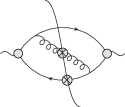
(a)

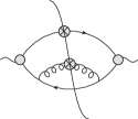
(b)

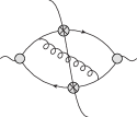
(c)

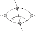
(d)

Figure 7: Representative cut real emission Feynman diagrams for the one-loop cross section in $e^{+}e^{-}$ annihilation where the final-state particles penetrate the two detectors. In (a) and (b) the detectors capture the gluon and (anti-)quark; in (c) and (d) they capture the quark and anti-quark.

We are interested in the charge-charge correlation at one-loop order, where the detectors are separated by a generic angle. In this case we do not consider the situation where both detectors are aligned and capture the same particle, i.e. if $\zeta=0$. At $\zeta\neq 0$, we also do not consider the pure virtual diagrams at this order. Their contribution is a contact term $\sim\delta(\zeta-1)$, since momentum conservation forces the two final-state particles to go back to back. For this reason we will focus on the process $\gamma^{*}(q)\rightarrow{q}(k_{1}){\bar{q}}(k_{2}){g}(k_{3})$ at tree level, whose contribution is a regular function for $0<\zeta<1$. First, we compute the matrix element of the initial state sourced by the vector electromagnetic current $J_{\mu}=\bar{\Psi}\gamma_{\mu}\Psi$ (with $\Psi,\bar{\Psi}$ standing for the quark/antiquark fields) and the three-particle final state. After summing over the final state helicities and taking the color trace, the matrix element squared reads

$$\sum_{\rm{helicity}}{\rm tr}\,|{\cal M}_{\mu}|^{2}={\sum_{\rm{helicity}}\rm tr}\,\big{|}\langle{0}|J_{\mu}(0)|{k_{1}\,k_{2}\,k_{3}}\rangle\big{|}^{2}$$

$$\hskip 14.22636pt={32\pi}{\alpha_{s}}N_{c}C_{F}\,Q_{f}^{2}\left[\frac{s_{23}}{s_{13}}+\frac{s_{13}}{s_{23}}+\frac{2q^{2}s_{12}}{s_{13}\,s_{23}}\right]\,,$$ (B.4)

where $\alpha_{s}={g^{2}}/({4\pi})$, and $Q_{f}$ is the (fractional) charge carried by a quark of a given flavor $f$. Let us introduce the dimensionless variables $\tau_{i},\;i=1,2,3$,

$$\hskip 14.22636pt\tau_{i}\equiv\frac{2q\cdot k_{i}}{q^{2}},\quad\text{so that}\quad\frac{s_{ij}}{q^{2}}=1-\tau_{n},\;\;n\neq i\neq j,\quad\text{and}\quad\tau_{1}+\tau_{2}+\tau_{3}=2\,.$$ (B.5)

In the center-of-mass frame $\tau_{i}$ defines the fraction of the total energy carried by the $i$th particle. The three $\tau-$variables also determine the angles between each pair of final-state particles. More explicitly,

$$\frac{2E_{i}}{q^{0}}=\tau_{i}\,,\quad\;\frac{1-\cos\theta_{ij}}{2}=\frac{1-\tau_{n}}{\tau_{i}\tau_{j}},\quad n\neq i\neq j\,.$$ (B.6)

The three-body final-state phase space is conveniently parametrized by the $\tau_{i}$’s,

$${\rm d}\Pi_{3}\equiv(2\pi)^{4}\delta^{4}(q-k_{1}-k_{2}-k_{3})\prod_{i=1}^{3}\frac{d^{4}k_{i}}{(2\pi)^{4}}2\pi\delta_{+}(k_{i}^{2})$$

$$=\frac{q^{2}}{(4\pi)^{5}}d\Omega_{1}d\phi_{12}\,d\tau_{1}d\tau_{2}d\tau_{3}\,\delta(2-\tau_{1}-\tau_{2}-\tau_{3})\prod_{i=1}^{3}\theta(\tau_{i})\theta(1-\tau_{i})\,,$$ (B.7)

where $\Omega_{1}$ is the direction of $\vec{k}_{1}$, and $\phi_{12}$ is the azimuthal angle of $\vec{k}_{2}$ in the coordinate system where $\vec{k}_{1}$ is the polar axis. To proceed, we combine the matrix element (B) and the phase-space measure (B), and thus define the tree-level differential cross section for $\gamma^{*}\rightarrow{q}_{f}{\bar{q}}_{f}{g}$ ($q_{f}/\bar{q}_{f}$ stands for (anti-)quark of a given flavor),

$$\frac{1}{\sigma_{0}}\frac{d\sigma^{f}_{\rm LO}}{d\tau_{1}d\tau_{2}}=\frac{\alpha_{s}}{2\pi}\,C_{F}\,\frac{Q_{f}^{2}}{\sum_{f}Q_{f}^{2}}\frac{\tau_{1}^{2}+\tau_{2}^{2}}{(1-\tau_{1})(1-\tau_{2})}\,.$$ (B.8)

Here $\sigma_{0}=\frac{N_{c}}{2\pi}\sum_{f}Q_{f}^{2}\,q^{2}$ is the Born-level total cross section where we sum over the flavors of the quarks.

Now we are ready to compute the charge-charge correlation. By definition, it measures the differential cross section weighted by the electric charge carried by particles $i$ and $j$ at a fixed angular separation (recall (B.3)),

$$F_{\rm{QQC}}(\zeta) \stackrel{{\scriptstyle\rm{LO}}}{{=}}2\zeta^{2}\sum_{f}\int_{0}^{1}d\tau_{1}\int_{1-\tau_{1}}^{1}\hskip-5.69046ptd\tau_{2}\,\delta\Big{(}\zeta-\frac{\tau_{1}+\tau_{2}-1}{\tau_{1}\tau_{2}}\Big{)}\cdot(-Q_{f})\cdot(Q_{f})\cdot\frac{1}{\sigma_{0}}\frac{d\sigma_{\rm LO}^{f}}{d\tau_{1}d\tau_{2}}\,.$$

Here we sum over unordered pairs $(ij)$ in the final state. The two-fold phase-space integral yields the one-loop charge-charge correlation

$$F_{\rm{QQC}}(\zeta) \stackrel{{\scriptstyle\rm{LO}}}{{=}}\frac{\alpha_{s}}{\pi}\,C_{F}\,R_{Q}\frac{2\log(1-\zeta)+\zeta(2+\zeta)}{\zeta(1-\zeta)}\,,$$ (B.9)

where $R_{Q}\equiv\frac{\sum_{f}Q_{f}^{4}}{\sum_{f}Q_{f}^{2}}$. This result agrees with (4.3), thus showing the consistency between the amplitude calculation and our approach based on correlation functions.

Appendix C Tensor reduction of the one-loop integrals

In order to evaluate the integrals with tensor numerators we need to reduce them to scalar integrals. We apply the following procedure for the tensor reduction. The most complicated tensors that we encounter have rank two. Poincaré invariance implies that the tensor integral is a sum of 10 tensor structures,

$$\int d^{4}x_{0}\frac{x^{\mu}_{0a_{1}}\,x^{\nu}_{0a_{2}}}{(x^{2}_{01})^{n_{1}}\,(x^{2}_{02})^{n_{2}}\,(x^{2}_{03})^{n_{3}}\,(x^{2}_{04})^{n_{4}}}=\sum_{k\neq a_{1},\,l\neq a_{2}}x_{k\,a_{1}}^{\mu}x_{l\,a_{2}}^{\nu}\,I_{k,l}+\delta^{\mu\nu}\,I_{0}\,,$$ (C.1)

where $I_{k,l}$ and $I_{0}$ are some scalar integrals. To find them we define the projectors

$$P^{\mu}_{k;a}= x_{ka}^{\mu}\,[(x_{i_{1}a}x_{i_{2}a})^{2}-x_{i_{1}a}^{2}x_{i_{2}a}^{2}]+x_{i_{1}a}^{\mu}\,[(x_{ka}x_{i_{1}a})x_{i_{2}a}^{2}-(x_{i_{1}a}x_{i_{2}a})(x_{ka}x_{i_{2}a})]$$

$$+x_{i_{2}a}^{\mu}\,[(x_{ka}x_{i_{2}a})x_{i_{1}a}^{2}-(x_{i_{1}a}x_{i_{2}a})(x_{ka}x_{i_{1}a})]\,,$$ (C.2)

where $k\neq a$ and $\{i_{1},i_{2},k,a\}$ is a permutation of $\{1,2,3,4\}$. They satisfy

$$P_{k;a}\cdot x_{ia}=0\qquad\text{for}\;\;i\neq k\,.$$ (C.3)

Then we define the set of 10 rank-two projectors

$$T^{\mu\nu}_{k,l}=P_{k;a_{1}}^{\mu}\,P_{l;a_{2}}^{\nu}\;,\qquad k\neq a_{1}\;,\quad l\neq a_{2}\,;$$

$$T^{\mu\nu}_{10}=-\delta^{\mu\nu}+\sum_{k\neq a_{1},\,l\neq a_{2}}\frac{(x_{ka_{1}}\cdot x_{la_{2}})}{(P_{k;a_{1}}\cdot x_{ka_{1}})(P_{l;a_{2}}\cdot x_{la_{2}})}P_{k;a_{1}}^{\mu}P_{l;a_{2}}^{\nu}\,.$$ (C.4)

The projector $T_{10}$ has the useful properties

$$T_{10}^{\mu\nu}\delta_{\mu\nu}=3-D\;,\qquad T_{10}^{\mu\nu}\,(x_{ka_{1}})_{\mu}(x_{la_{2}})_{\nu}=0\,.$$ (C.5)

Now we project eq. (C.1) with the 10 projectors,

$$\int d^{4}x_{0}\frac{x^{\mu}_{0a_{1}}\,(T_{k,l})_{\mu\nu}\,x^{\nu}_{0a_{2}}}{(x^{2}_{01})^{n_{1}}\,(x^{2}_{02})^{n_{2}}\,(x^{2}_{03})^{n_{3}}\,(x^{2}_{04})^{n_{4}}}=x_{k\,a_{1}}^{\mu}(T_{k,l})_{\mu\nu}\,x_{l\,a_{2}}^{\nu}\,I_{k,l}+T_{k,l}^{\mu\nu}\delta_{\mu\nu}\,I_{0}\;,$$

$$\int d^{4}x_{0}\frac{x^{\mu}_{0a_{1}}\,(T_{10})_{\mu\nu}\,x^{\nu}_{0a_{2}}}{(x^{2}_{01})^{n_{1}}\,(x^{2}_{02})^{n_{2}}\,(x^{2}_{03})^{n_{3}}\,(x^{2}_{04})^{n_{4}}}=(3-D)\,I_{0}\,.$$ (C.6)

This triangular system of equations is solved immediately and we find the scalar integrals $I_{k,l}$ and $I_{10}$.

Appendix D Rules for taking double discontinuity

Starting from the master formula, $\text{dDisc}[w^{-p+\epsilon}]=2\sin^{2}(\pi\epsilon)w^{-p+\epsilon}$ , we can generate logarithms terms via derivatives and work out the double discontinuity of pole times powers of logarithms (e.g. the integrand in (4.2.2)) efficiently. For $p,n,m\in N$, the general formula is

$$\text{dDisc}_{w=0}[w_{+}^{-p+\epsilon}\ln^{m}w_{+}]\ln^{n}w_{+}$$

$$=\partial^{m}_{\epsilon}\left[2\sin^{2}(\pi\epsilon)\,\partial^{n}_{\epsilon}\,\frac{\Gamma(\epsilon-p+1)}{\Gamma(\epsilon)}\,\partial_{w}^{p-1}\hskip-2.84544pt\left(\frac{1}{\epsilon}\delta(w)+\sum_{k=0}\frac{\epsilon^{k}}{k!}w^{-1}_{+}\ln^{k}w_{+}\right)\right]\,.$$ (D.1)

Taking the limit $\epsilon\to 0$, we obtain the double discontinuity of a $p-$th degree pole times multiple powers of logarithms. Here are a few examples of the application of (D) for $n=0,1$, $m=0,1$:

$$\text{dDisc}\,w_{+}^{-p+\epsilon}\ \stackrel{{\scriptstyle\epsilon\to 0}}{{\longrightarrow}}\ 0\,,$$

$$\text{dDisc}[w_{+}^{-p+\epsilon}]\ln w_{+}\ \stackrel{{\scriptstyle\epsilon\to 0}}{{\longrightarrow}}\ -2\pi^{2}\frac{(-1)^{p-1}}{(p-1)!}\,\delta^{(p-1)}(w)\,,$$

$$\text{dDisc}[w_{+}^{-p+\epsilon}\ln w_{+}]\ \stackrel{{\scriptstyle\epsilon\to 0}}{{\longrightarrow}}\ 2\pi^{2}\frac{(-1)^{p-1}}{(p-1)!}\,\delta(w)\,,$$

$$\text{dDisc}[w_{+}^{-p+\epsilon}\ln w_{+}]\ln w_{+}\ \stackrel{{\scriptstyle\epsilon\to 0}}{{\longrightarrow}}\ 0\,.$$ (D.2)

Applying these formulas to the integral in (4.2.2) we find

$$G(\gamma) =2\pi^{2}\sum_{p}\frac{1}{(p-1)!}\left[\partial_{\bar{z}}^{p-1}B_{0}(\bar{z},\gamma)-\partial_{\bar{z}}^{p-1}A_{1}(\bar{z},\gamma)\right]\bigg{|}_{\bar{z}=1}$$

$$=2\pi^{2}\,\text{Res}_{\bar{z}=1}\left[B_{0}(\bar{z},\gamma)-A_{1}(\bar{z},\gamma)\right]\,,$$ (D.3)

as stated in (4.2.2).

Appendix E Fourier transform in eq. (4.3)

We start with the Fourier integral

$$\int d^{4}x\frac{e^{iqx}\gamma^{j}}{(x^{2}-i\epsilon x^{0})^{3}\gamma^{3}}=-\frac{\pi^{3}q^{2}\zeta^{3-j}}{2\Gamma(j)\Gamma(5-j)}\,{}_{2}F_{1}\left(2-j,2-j;5-j|\zeta\right)\,,$$ (E.1)

with $\gamma$ and $\zeta$ defined in (4.6) and (2.33), respectively. This integral is obtained using Schwinger’s parametrization, with the help of the formula Belitsky:2013xxa

$$\int_{0}^{\infty}d\omega d\omega^{\prime}\,(\omega\omega^{\prime})^{a}\left[(q-n\omega-n^{\prime}\omega^{\prime})^{2}\right]^{b}\theta((q-n\omega-n^{\prime}\omega^{\prime})^{2})\theta(q_{0}-n_{0}\omega-n^{\prime}_{0}\omega^{\prime})$$

$$=\frac{\Gamma^{2}(a+1)\Gamma(b+1)}{\Gamma(2a+b+3)}\zeta^{a+1}(q^{2})^{a+b+1}(2(nn^{\prime}))^{-a-1}\,{}_{2}F_{1}\left(a+1,a+1;2a+b+3|\zeta\right)\,.$$ (E.2)

Using (E.1) we find

$$\int d^{4}x\frac{e^{iqx}}{(x^{2}-i\epsilon x^{0})^{3}\gamma^{3}}=0\,,$$

$$\int d^{4}x\frac{e^{iqx}\gamma}{(x^{2}-i\epsilon x^{0})^{3}\gamma^{3}}=-\frac{\pi^{3}q^{2}}{2\zeta}[(\zeta-2)\log(1-\zeta)-2\zeta]\,,$$

$$\int d^{4}x\frac{e^{iqx}\log(\gamma)}{(x^{2}-i\epsilon x^{0})^{3}\gamma^{3}}=-\frac{\pi^{3}q^{2}}{8\zeta(1-\zeta)}[\zeta(6-5\zeta)+(2\zeta^{2}-8\zeta+6)\log(1-\zeta)]\,.$$ (E.3)

To obtain the last identity we acted with $\partial_{j}|_{j=0}$ on both sides of (E.1).

The Fourier transform of the dilogarithm term in eq. (4.17) is found with the help of the relation Korchemsky:2015ssa

$$\left[\gamma^{2}(1-\gamma)^{2}G^{{}^{\prime\prime}}(\gamma)\right]^{{}^{\prime\prime}}=\frac{1}{16}(x^{2})^{3}\Box^{2}_{x}\frac{G(\gamma)}{x^{2}}\,.$$ (E.4)

We substitute $G(\gamma)=\frac{1}{\gamma}{\rm Li}_{2}\left(1-\frac{1}{\gamma}\right)$ in this equation and Fourier transform both sides,

$$\int d^{4}x\frac{e^{iqx}}{(x^{2}-i\epsilon x^{0})^{3}\gamma^{3}}\left[4{\rm Li}_{2}\left(1-\frac{1}{\gamma}\right)+12\log(\gamma)+6\gamma-13\right]$$

$$=\frac{(q^{2})^{2}}{16}\int d^{4}x\frac{e^{iqx}}{x^{2}-i\epsilon x^{0}}\frac{1}{\gamma}{\rm Li}_{2}\left(1-\frac{1}{\gamma}\right)=\frac{\pi^{3}q^{2}}{2}\frac{\zeta\log(1-\zeta)}{1-\zeta}\,,$$ (E.5)

where the second relation can be found in Belitsky:2013xxa . Thus we get

$$\int d^{4}x\frac{e^{iqx}}{(x^{2}-i\epsilon x^{0})^{3}\gamma^{3}}{\rm Li}_{2}\left(1-\frac{1}{\gamma}\right)=\frac{\pi^{3}q^{2}}{2}\frac{3(2-\zeta)\zeta+(6-6\zeta+\zeta^{2})\log(1-\zeta)}{\zeta(1-\zeta)}\,.$$ (E.6)

Combining these steps yields (4.3) in the main text.

References

• (1) G. C. Fox and S. Wolfram, “Observables for the Analysis of Event Shapes in e+ e- Annihilation and Other Processes,” Phys. Rev. Lett.  41 (1978) 1581.
• (2) C. L. Basham, L. S. Brown, S. D. Ellis and S. T. Love, “Energy Correlations in electron - Positron Annihilation: Testing QCD,” Phys. Rev. Lett.  41 (1978) 1585.
• (3) C. L. Basham, L. S. Brown, S. D. Ellis and S. T. Love, “Energy Correlations in electron-Positron Annihilation in Quantum Chromodynamics: Asymptotically Free Perturbation Theory,” Phys. Rev. D 19 (1979) 2018.
• (4) R. K. Ellis, D. A. Ross and A. E. Terrano, “The Perturbative Calculation of Jet Structure in e+ e- Annihilation,” Nucl. Phys. B 178 (1981) 421.
• (5) Z. Kunszt, P. Nason, G. Marchesini, B.R. Webber, “QCD at LEP,” In Geneva 1989, Proceedings, Z physics at LEP 1, vol. 1, pp. 373-453.
• (6) Z. Kunszt, D.E. Soper, “Calculation of jet cross sections in hadron collisions at order $\alpha_{s}^{3}$,” Phys. Rev. D 46 (1992) 192.
• (7) O. Biebel, “Experimental tests of the strong interaction and its energy dependence in electron positron annihilation,” Phys. Rept.  340 (2001) 165.
• (8) A. V. Belitsky, G. P. Korchemsky and G. F. Sterman, “Energy flow in QCD and event shape functions,” Phys. Lett. B 515 (2001) 297 [hep-ph/0106308].
• (9) L. J. Dixon, M. X. Luo, V. Shtabovenko, T. Z. Yang and H. X. Zhu, “Analytical Computation of Energy-Energy Correlation at Next-to-Leading Order in QCD,” Phys. Rev. Lett.  120, no. 10, 102001 (2018) [arXiv:1801.03219 [hep-ph]].
• (10) E. W. N. Glover and M. R. Sutton, “The Energy-energy correlation function revisited,” Phys. Lett. B 342 (1995) 375 [hep-ph/9410234].
• (11) A. V. Belitsky, S. Hohenegger, G. P. Korchemsky, E. Sokatchev and A. Zhiboedov, “Energy-Energy Correlations in N=4 Supersymmetric Yang-Mills Theory,” Phys. Rev. Lett.  112 (2014) 7, 071601 [arXiv:1311.6800 [hep-th]].
• (12) V. Del Duca, C. Duhr, A. Kardos, G. Somogyi, Z. Szőr, Z. Trócsányi and Z. Tulipánt, “Jet production in the CoLoRFulNNLO method: event shapes in electron-positron collisions,” Phys. Rev. D 94 (2016) no.7, 074019 [arXiv:1606.03453 [hep-ph]].
• (13) J. M. Henn, E. Sokatchev, K. Yan and A. Zhiboedov, “Energy-energy correlation in $N$=4 super Yang-Mills theory at next-to-next-to-leading order,” Phys. Rev. D 100 (2019) no.3, 036010 [arXiv:1903.05314 [hep-th]].
• (14) D. M. Hofman and J. Maldacena, “Conformal collider physics: Energy and charge correlations,” JHEP 0805 (2008) 012 [arXiv:0803.1467 [hep-th]].
• (15) A. V. Belitsky, S. Hohenegger, G. P. Korchemsky, E. Sokatchev and A. Zhiboedov, “From correlation functions to event shapes,” Nucl. Phys. B 884 (2014) 305 [arXiv:1309.0769 [hep-th]].
• (16) A. V. Belitsky, S. Hohenegger, G. P. Korchemsky, E. Sokatchev and A. Zhiboedov, “Event shapes in $\mathcal{N}=4$ super-Yang-Mills theory,” Nucl. Phys. B 884 (2014) 206 [arXiv:1309.1424 [hep-th]].
• (17) G. P. Korchemsky, “Energy correlations in the end-point region,” JHEP 2001 (2020) 008 [arXiv:1905.01444 [hep-th]].
• (18) L. J. Dixon, I. Moult and H. X. Zhu, “Collinear limit of the energy-energy correlator,” Phys. Rev. D 100 (2019) no.1, 014009 [arXiv:1905.01310 [hep-ph]].
• (19) M. Kologlu, P. Kravchuk, D. Simmons-Duffin and A. Zhiboedov, “The light-ray OPE and conformal colliders,” arXiv:1905.01311 [hep-th].
• (20) A. V. Belitsky, S. Hohenegger, G. P. Korchemsky and E. Sokatchev, “N=4 superconformal Ward identities for correlation functions,” Nucl. Phys. B 904 (2016) 176 [arXiv:1409.2502 [hep-th]].
• (21) G. P. Korchemsky and E. Sokatchev, “Four-point correlation function of stress-energy tensors in $\mathcal{N}=4$ superconformal theories,” JHEP 1512 (2015) 133 [arXiv:1504.07904 [hep-th]].
• (22) G. M. Sotkov and R. P. Zaikov, “On the Structure of the Conformal Covariant $N$ Point Functions,” Rept. Math. Phys.  19, 335 (1984).
• (23) A. Dymarsky, “On the four-point function of the stress-energy tensors in a CFT,” JHEP 1510 (2015) 075 [arXiv:1311.4546 [hep-th]].
• (24) P. Kravchuk and D. Simmons-Duffin, “Counting Conformal Correlators,” JHEP 1802 (2018) 096 [arXiv:1612.08987 [hep-th]].
• (25) D. Karateev, “Kinematics of 4D Conformal Field Theories,” PhD thesis, unpublished.
• (26) F. R. Ore, Jr. and G. F. Sterman, “An Operator Approach To Weighted Cross-sections,” Nucl. Phys. B 165 (1980) 93.
• (27) N.A. Sveshnikov, F.V. Tkachov, “Jets and quantum field theory,” Phys. Lett. B 382 (1996) 403 [hep-ph/9512370].
• (28) G. P. Korchemsky, G. Oderda and G. F. Sterman, “Power corrections and nonlocal operators,” AIP Conf. Proc.  407 (1997) no.1, 988 [hep-ph/9708346].
• (29) G.P. Korchemsky, G.F. Sterman, “Power corrections to event shapes and factorization,” Nucl. Phys. B 555 (1999) 335 [hep-ph/9902341].
• (30) A.V. Belitsky, G.P. Korchemsky, G. Sterman, “Energy flow in QCD and event shape functions,” Phys. Lett. B 515 (2001) 297 [hep-ph/0106308].
• (31) R. K. Ellis, W. J. Stirling and B. R. Webber, “QCD and collider physics,” Camb. Monogr. Part. Phys. Nucl. Phys. Cosmol.  8 (1996) 1.
• (32) G. Mack, “D-independent representation of Conformal Field Theories in D dimensions via transformation to auxiliary Dual Resonance Models. Scalar amplitudes,” arXiv:0907.2407 [hep-th].
• (33) S. Caron-Huot, “Analyticity in Spin in Conformal Theories,” JHEP 1709 (2017) 078 [arXiv:1703.00278 [hep-th]].
• (34) L. F. Alday and S. Caron-Huot, “Gravitational S-matrix from CFT dispersion relations,” JHEP 1812 (2018) 017 [arXiv:1711.02031 [hep-th]].
• (35) B. Eden, C. Schubert, E. Sokatchev, “Three loop four point correlator in N=4 SYM,” Phys. Lett. B 482 (2000) 309 [hep-th/0003096].
• (36) B. Eden, G. P. Korchemsky and E. Sokatchev, “From correlation functions to scattering amplitudes,” JHEP 1112 (2011) 002 [arXiv:1007.3246 [hep-th]].
• (37) Z. Bern and A. G. Morgan, “Massive loop amplitudes from unitarity,” Nucl. Phys. B 467 (1996) 479 [hep-ph/9511336].
• (38) N. I. Usyukina and A. I. Davydychev, “Exact results for three and four point ladder diagrams with an arbitrary number of rungs,” Phys. Lett. B 305 (1993) 136.
• (39) N. I. Usyukina and A. I. Davydychev, “Some exact results for two loop diagrams with three and four external lines,” Phys. Atom. Nucl.  56 (1993) 1553 [Yad. Fiz.  56N11 (1993) 172] [hep-ph/9307327].
• (40) A. Banfi, G. P. Salam and G. Zanderighi, “Phenomenology of event shapes at hadron colliders,” JHEP 1006 (2010) 038 [arXiv:1001.4082 [hep-ph]].
• (41) J. Drummond, C. Duhr, B. Eden, P. Heslop, J. Pennington and V. A. Smirnov, “Leading singularities and off-shell conformal integrals,” JHEP 1308, 133 (2013) [arXiv:1303.6909 [hep-th]].
• (42) B. Eden and V. A. Smirnov, “Evaluating four-loop conformal Feynman integrals by D-dimensional differential equations,” JHEP 1610, 115 (2016) [arXiv:1607.06427 [hep-th]].
• (43) V. N. Velizhanin, “Non-planar anomalous dimension of twist-2 operators: higher moments at four loops,” Nucl. Phys. B 885, 772 (2014) [arXiv:1404.7107 [hep-th]].
• (44) F. Herzog, S. Moch, B. Ruijl, T. Ueda, J. A. M. Vermaseren and A. Vogt, “Five-loop contributions to low-N non-singlet anomalous dimensions in QCD,” Phys. Lett. B 790, 436 (2019) [arXiv:1812.11818 [hep-ph]].
• (45) J. M. Drummond, J. Henn, V. A. Smirnov and E. Sokatchev, “Magic identities for conformal four-point integrals,” JHEP 0701, 064 (2007) [hep-th/0607160].
• (46) O. Schnetz, “Graphical functions and single-valued multiple polylogarithms,” Commun. Num. Theor. Phys.  08, 589 (2014) [arXiv:1302.6445 [math.NT]].
• (47) V. M. Braun, G. P. Korchemsky and D. Müller, “The Uses of conformal symmetry in QCD,” Prog. Part. Nucl. Phys.  51, 311 (2003) [hep-ph/0306057].
• (48) A. Grozin, J. M. Henn, G. P. Korchemsky and P. Marquard, “The three-loop cusp anomalous dimension in QCD and its supersymmetric extensions,” JHEP 1601, 140 (2016) [arXiv:1510.07803 [hep-ph]].
• (49) V. M. Braun, A. N. Manashov, S. O. Moch and M. Strohmaier, “Conformal symmetry of QCD in $d$-dimensions,” Phys. Lett. B 793, 78 (2019) [arXiv:1810.04993 [hep-th]].
• (50) H. Chen, M. X. Luo, I. Moult, T. Z. Yang, X. Zhang and H. X. Zhu, “Three Point Energy Correlators in the Collinear Limit: Symmetries, Dualities and Analytic Results,” arXiv:1912.11050 [hep-ph].
• (51) A. Galperin, E. Ivanov, S. Kalitsyn, V. Ogievetsky and E. Sokatchev, “Unconstrained N=2 Matter, Yang-Mills and Supergravity Theories in Harmonic Superspace,” Class. Quant. Grav.  1 (1984) 469 Erratum: [Class. Quant. Grav.  2 (1985) 127].
• (52) A. S. Galperin, E. A. Ivanov, V. I. Ogievetsky and E. S. Sokatchev, “Harmonic superspace,” Cambridge, UK: Univ. Pr. (2001) 306 p