Greybody Factor for Quintessential Kerr-Newman Black Hole

Abstract

In this paper, we formulate an analytic expression of the greybody factor for the Kerr-Newman black hole in the presence of the quintessential field. Primarily, we analyze the profile of effective potential by transforming the radial equation of motion into standard Schr$\ddot{o}$dinger form through tortoise coordinate. The two asymptotic solutions, in the form of hypergeometric functions, are computed at distinct radial regions such as a black hole and cosmological horizons determined by the quintessence. To extend the viability over the whole radial regime, we match the analytical solutions smoothly in an intermediate region by using a semi-classical approach. We also calculate the emission rates and absorption cross-section for the massless scalar fields to elaborate on the significance of our result. It is found that the electromagnetic force together with the gravitational pull of black hole maximizes the effective potential and consequently, decreases the emission process of scalar field particles.

Keywords: Black hole; Greybody factor; Klein-Gordon equation; Dark energy; Quintessence; Electromagnetic field.
PACS: 04.70.Dy; 52.25.Tx; 04.70.-s; 95.36.+x; 03.50.De.

1 Introduction

After the remarkable discovery of Hawking radiation [1], the scattering of the material field from various black holes (BHs) has become one of the interesting topics of strong gravitational fields. These thermal spectra of radiations as the dividing line between classical general relativity and quantum field theory may play an effective role to resolve the mysterious nature of BHs. Due to quantum mechanical effects, virtual particles created at the event horizon spread out in the surrounding space that lead to decrease in the BH mass and finally to its eventual evaporation. The geometry outside the BH horizon has a significant impact on the emission rate of scalar particles. In fact, the spacetime outside the boundary of BH will work as a potential barrier for the emitted Hawking radiation. Consequently, the radiation spectrum at the horizon is exactly equal to the blackbody while the spectrum recorded by the distant observer will depict different scenario. Mathematically, the relative relation between the blackbody radiation and asymptotic radiation spectra can be expressed as

$$\gamma(w)=\left(\frac{|\tilde{\emph{A}}_{l,m}|^{2}d^{3}k}{(e^{\frac{w}{T_{H}}}\pm 1)(2\pi)^{3}}\right),$$

where $T_{H}$ denotes the Hawking temperature and $|\tilde{\emph{A}}_{l,m}|^{2}$ is dubbed as greybody factor which is a frequency-dependent quantity. The greybody factor (rate of absorption probability) is defined as the probability for an incoming wave from infinity to be absorbed by the BH which is directly related to the absorption cross-section [2]-[5].

In astrophysics, the study of reflection as well as transmission coefficients of the waves has gained much attention. Konoplya [6] computed the effective potential as well as quasinormal modes associated with the decay of the massless scalar field for small Schwarzschild-anti de Sitter BH. Konoplya and Zhidenko [7, 8] analyzed the quasinormal modes of various BHs through numerical and analytical techniques such as WKB method, integration of the wavelike equations, Frobenius method, Fit and interpolation approaches, etc. Ngampitipan and Boonserm [9] obtained rigorous bounds on the transmission coefficient for Reissner-Nordstr$\ddot{o}$n (RN) BH by using $2\times 2$ transfer matrices. Boonserm et al. [10] established some bounds on the absorption probability associated with scalar field excitations for the Kerr-Newman BH. Toshmatov et al. [11] computed the greybody factors for regular BH spacetimes and found that charge parameter decreases the transmission rate of the incident wave. Ahmed and Saifullah [12] studied the propagation of massless scalar fields in the background of charged string theory and obtained an analytic expression of the greybody factor in the low-energy approximation. They also derived a general expression of absorption probability for RN-de Sitter BH [13]. Recently, Dey and Chakrabarti [14] calculated quasinormal modes as well as greybody factor for the Bardeen-de Sitter BH through electromagnetic perturbations.

Recent astronomical observations suggest that our universe is expanding at an accelerating rate, driven by some unknown exotic component dubbed as dark energy (DE). Despite the enormous cosmological pieces of evidence, the origin as well as essential characteristics of DE is still elusive and has become a source of vivid debate. There are different DE models such as cosmological constant $\Lambda$, quintessence energy, etc. that can effectively describe the dynamics of the current universe. The cosmological constant with negative pressure has the same value everywhere in space, i.e., $\Lambda\approx 1.3\times 10^{-56}$cm^-2 [15] which changes the spacetime structure of the compact objects. The quintessence energy is inhomogeneous as well as dynamical scalar field which can be characterized by the equation of state $\omega_{q}=\frac{P_{q}}{\rho_{q}}$ with $-1<\omega_{q}<-\frac{1}{3}$, where $P_{q}$ and $\rho_{q}$ denote the pressure and energy density, respectively. Similar to the cosmological constant, the cosmological horizon exists in the BH spacetime immersed in the quintessential field.

In the presence of quintessential DE, the first-ever BH solution was formulated by Kiselev [16]. He derived spherically symmetric exact solutions of the field equations for charged as well as uncharged BH surrounded by the quintessence. Following this technique, various BH solutions have been constructed in the background of quintessential field [17]. Chen et al. [18] examined the Hawking radiation spectra as well as greybody factor for d-dimensional BH by using an equation of state of quintessence matter and found that the luminosity of radiation depends upon $|\omega_{q}|$. Hao et al. [19] investigated the absorption cross-section and absorption probability for the Schwarzschild BH in the presence of quintessence matter. Saleh et al. [20] studied the quasinormal modes as well as Hawking radiation for quintessential RN BH. Chakrabarty et al. [21] analyzed the quasinormal modes as well as greybody factor for the emission of scalar particles around a nonlinear magnetic-charged BH surrounded by quintessence.

In this paper, we study an analytic form of the greybody factor in the gravitational background corresponding to quintessential charged rotating BH. The paper is outlined as follows. In the next section, we evaluate the radial part of Klein-Gordon equation as well as Schr$\ddot{o}$dinger equation to analyze the effective potential for the massless scalar fields. Section 3 deals with two analytic solutions of the radial equation of motion evaluated at two specific radial regimes. In section 4, we extrapolate these asymptotic solutions to attain an analytic expression of the greybody factor. We also calculate the energy emission rate and absorption cross-section for the scalar field particles. Finally, we summarize our results in the last section.

2 Klein-Gordon Equation and Effective Potential

The accelerated expansion of the universe could be the result of quintessence matter which permeates the whole space. The quintessential field around BH alters its spacetime properties as well as asymptotic features of the cosmological horizon. Newman and Janis [22] obtained Kerr BH solution from the Schwarzschild spacetime by employing complex transformation within the framework of Newman-Penrose formalism [23]. The same procedure was adopted to generate the Kerr-Newman BH from the RN metric [24]. The Newman-Janis algorithm (NJA) has been contemplated as a favorable approach to obtain new rotating solutions of the Einstein field equations [25, 26]. Toshmatov et al. [27] derived the quintessential rotating BH solution by applying NJA on the spherically symmetric BH. Using the same technique, Xu and Wang [28] studied the Kerr-Newman solution in the presence of quintessential DE. In the Boyer-Lindquist coordinates, the Kerr-Neuman metric surrounded by quintessence can be expressed as

$$ds^{2}=-F(r,\theta)dt^{2}+\frac{1}{G(r,\theta)}dr^{2}+\Sigma(r,\theta)d\theta^{2}+H(r,\theta)d\phi^{2}-2K(r,\theta)dtd\phi,$$ (1)

where

$$F(r,\theta) = \frac{\Delta(r)-a_{0}^{2}\sin^{2}\theta}{\Sigma(r,\theta)},\quad G(r,\theta)=\frac{\Delta(r)}{\Sigma(r,\theta)},\quad\Sigma(r,\theta)=r^{2}+a_{0}^{2}\cos^{2}\theta,$$

$$H(r,\theta) = \frac{\sin^{2}\theta\left((r^{2}+a_{0}^{2})^{2}-\Delta(r)a_{0}^{2}\sin^{2}\theta\right)}{\Sigma(r,\theta)},$$

$$K(r,\theta) = \frac{a_{0}\sin^{2}\theta(r^{2}+a_{0}^{2}-\Delta(r))}{\Sigma(r,\theta)},\quad\Delta(r)=r^{2}+a_{0}^{2}+Q^{2}-2rM-\alpha r^{1-3\omega_{q}}.$$

Here $a_{0}$ corresponds to the rotation parameter, $M$ and $Q$ are the gravitational mass and total charge of BH, respectively, $\omega_{q}$ is the dimensionless state parameter and $\alpha$ is the quintessence parameter which determines the magnitude of quintessence field around a BH, satisfying the inequality [28]

$$\alpha\leq\frac{2}{1-3\omega_{q}}8^{\omega_{q}}.$$ (2)

This relation holds when the cosmological horizon determined by quintessential DE exists. It is noted that charge does not affect the range of $\alpha$, it remains the same for charge as well as uncharged scenario. For $\alpha=0$, the line element (1) reduces to Kerr-Newman BH which further leads to Kerr solution in the absence of charge parameter. The horizons can be computed by the constraint

$$\Delta(r)=0=r^{2}-2rM+a_{0}^{2}+Q^{2}-\alpha r^{1-3\omega_{q}}.$$ (3)

The most appropriate method to study perturbations near a spacetime generated by a BH is to allow probe fields to be perturbed by such spacetime without reacting on it. If there is no effect of the field on the spacetime, the perturbations of BH can be studied not only by adding the perturbation terms, but also by introducing fields to the spacetime [8]. In general, for a scalar field, this leads to find solutions for the Klein-Gordon equation with a well-defined boundary condition. To analyze the emission of scalar fields $\Psi$ from a BH, we first derive the Klein-Gordon equation of a scalar wave propagating in the gravitational background (1). We assume that massless particles are only minimally coupled to gravity and do not involve in any other interaction. In this scenario, the equation of motion for the curved spacetime is expressed as

$$\nabla_{\mu}\nabla^{\mu}\Psi=\partial_{\mu}[\sqrt{-g}g^{\mu\nu}\partial_{\nu}\Psi(t,r,\theta,\phi)]=0,$$ (4)

which, through Eq.(1), reduces to

$$\sqrt{-g}\left(\frac{-H}{K^{2}+FH}\right)\partial_{tt}\Psi+(\sqrt{-g}G\partial_{r}\Psi)_{,r}+(\sqrt{-g}\frac{1}{\Sigma}\partial_{\theta}\Psi)_{,\theta}$$

$$+\sqrt{-g}\left(\frac{F}{K^{2}+FH}\right)\partial_{\phi\phi}\Psi+2\sqrt{-g}\left(\frac{-K}{K^{2}+FH}\right)\partial_{t}\partial_{\phi}\Psi=0.$$ (5)

Using the separation of variables ansatz

$$\Psi(t,r,\theta,\phi)=\exp(-\iota wt)\exp(\iota m\phi)R_{wlm}(r)Q^{m}_{l}(\theta,a_{0}w),$$

where $w$ denotes the frequency of wave and $Q^{m}_{l}(\theta,a_{0}w)$ corresponds to the angular spheroidal functions [29], $R_{wlm}$ and $Q^{m}_{l}$ are obtained as the solutions of the following decoupled equations

$$\frac{\partial}{\partial r}(\Delta\frac{\partial R_{wlm}}{\partial r})+\left[\frac{1}{\Delta}(w^{2}(r^{2}+a_{0}^{2})^{2}+a_{0}^{2}m^{2}-2a_{0}wm(2rM-Q^{2}+\alpha r^{1-3\omega_{q}}))\right.$$

$$\left.-a_{0}^{2}w^{2}-\lambda_{l}^{m}\right]R_{wlm}=0,$$ (6)

$$\frac{1}{\sin\theta}\frac{\partial}{\partial\theta}\left(\sin\theta\frac{\partial Q^{m}_{l}}{\partial\theta}\right)+(-\frac{m^{2}}{\sin^{2}\theta}+w^{2}a_{0}^{2}\cos^{2}\theta+\lambda_{l}^{m})Q^{m}_{l}(\theta,a_{0}w)=0.$$ (7)

Here $\lambda_{l}^{m}$ are the angular eigenvalues whose analytic form in terms of power series [30] can be written as

$$\lambda_{l}^{m}=\sum_{n=0}^{\infty}\textit{f}_{~{}n}^{~{}lm}(a_{0}w)^{n}.$$ (8)

The angular eigenvalue provides a connection between radial and angular equations. In general, its analytic expression cannot be written in a closed form. For simplicity, it is sufficient to keep the finite number of terms and truncate the series at fourth order given as follows

$$\lambda_{l}^{m}=l(l+1)+\frac{2m^{2}-2l(l+1)+1}{(2l-1)(2l+3)}(a_{0}w)^{2}+O((a_{0}w)^{4}),$$ (9)

with $\textit{f}_{~{}1}^{~{}lm}=\textit{f}_{~{}3}^{~{}lm}=0$. The parameter $l$ depicts the orbital angular momentum with non-negative integral values and $m$ takes any integer value providing $l\geq|m|$ and $\frac{l-|m|}{2}\in\{0,\mathbb{Z}^{+}\}$.

To derive the greybody factor for the massless scalar fields, we determine an analytic solution of radial equation (6) by using the above-mentioned power series expression. Before attempting to solve it analytically, we first analyze the profile of effective potential which characterizes the emission process. Defining a new radial function

$$R_{wlm}(r)=\frac{U_{wlm}(r)}{\sqrt{r^{2}+a_{0}^{2}}},$$ (10)

and use tortoise coordinate $x_{*}$ as

$$\frac{dx_{*}}{dr}=\frac{r^{2}+a_{0}^{2}}{\Delta(r)},$$ (11)

we get the following relations

$$\frac{d}{dx_{*}}=\frac{\Delta(r)}{r^{2}+a_{0}^{2}}\frac{d}{dr},\quad\frac{d^{2}}{dx_{*}^{2}}=\left(\frac{\Delta(r)}{r^{2}+a_{0}^{2}}\right)^{2}\frac{d^{2}}{dr^{2}}+\left(\frac{\Delta(r)}{r^{2}+a_{0}^{2}}\right)\frac{d}{dr}\left(\frac{\Delta(r)}{r^{2}+a_{0}^{2}}\right)\frac{d}{dr}.$$ (12)

The tortoise coordinate extends the range of the model between $-\infty$ to $\infty$ whereas the Regge-Wheeler equation (6) is confined only to regions located outside the BH horizon. In this scenario, Eq.(6) can be rewritten in the standard Schr$\ddot{o}$dinger equation as

$$(\frac{d^{2}}{dx_{*}^{2}}-V_{eff})U_{wlm}(r)=0,$$ (13)

where the effective potential has the form

$$V_{eff}=\{(r^{2}+a^{2})^{\frac{1}{2}}\frac{d}{dr}\left[\frac{r\Delta(r)}{(r^{2}+a_{0}^{2})^{\frac{3}{2}}}\right]-\frac{1}{\Delta}[w^{2}(r^{2}+a_{0}^{2})^{2}+a_{0}^{2}m^{2}-2a_{0}wm$$

$$\times(2Mr-Q^{2}+\alpha r^{1-3\omega_{q}})]+a_{0}^{2}w^{2}+l(l+1)+\frac{2m^{2}-2l(l+1)+1}{(2l-1)(2l+3)}(a_{0}w)^{2}\}\frac{\Delta(r)}{(r^{2}+a_{0}^{2})^{2}}.$$

(14)

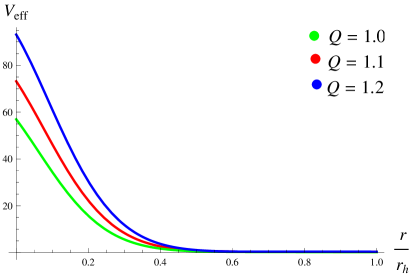
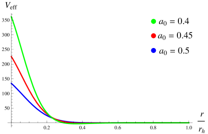
Figure 1: Effective potential for massless scalar fields corresponding to $a_{0}=0.6$ (left plot) and $Q=1$ (right plot) with $m=l=M=1$, $\alpha=0.01$, $\omega_{q}=-0.6$ and $w=0.1$.

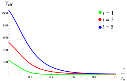
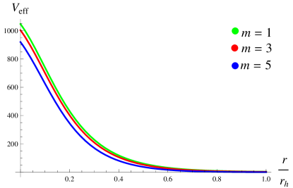
Figure 2: Effective potential for massless scalar fields corresponding to $m=1$ (left plot) and $l=5$ (right plot) with $Q=M=1$ and $w=0.1$, $a_{0}=0.45$, $\omega_{q}=-0.6$ and $\alpha=0.01$.

We see that the effective potential approaches to zero as $x_{*}\rightarrow\pm\infty$. For graphical analysis, we display the dependence of effective potential on different parameters in the form of Figures 1-2. Primarily, we set the parameters $m=l=1=M$, $\alpha=0.01$, $\omega_{q}=-0.6$ and sketch the plots for different choices of charge and rotation parameters. It is found that the gravitational barrier increases gradually with the increase in charge quantity (left plot of Figure 1) which shows that the inclusion of charge enhances the gravitational pull of BH. Thus, both forces (electromagnetic and gravitational forces) act in the same direction which ultimately increase the effective potential and reduce the emission of scalar fields. As a result, the greybody factor will decrease corresponding to larger choices of $Q$. In the right plot of Figure 1, we display the profile of effective potential in terms of rotation parameter. We observe that the potential barrier increases for smaller modes of $a_{0}$ leading to the deduction of emission process. The dependence of the gravitational barrier on angular momentum numbers is shown in Figure 2. It is noted that higher values of the potential are obtained for larger modes of partial wave $l$ whereas the parameter $m$ has an inverse impact on the effective potential, i.e., smaller values of $m$ yield higher spikes of the potential.

3 Greybody Factor

In this section, we compute an analytic expression of the greybody factor by solving the radial equation at specific radial regimes such as close to the BH horizon and cosmological horizon determined by the quintessence. We then use a semi-classical approach to smoothly match these solutions in the low rotation regions.

3.1 Analytic Solutions

For the domain near to the BH event horizon $r\sim r_{h}$, we employ the transformation

$$r\rightarrow S=\frac{r^{2}+a_{0}^{2}+Q^{2}-2rM-\alpha r^{1-3\omega_{q}}}{r^{2}+a_{0}^{2}-\alpha r^{1-3\omega_{q}}},$$ (15)

which satisfies the relation

$$\frac{dS}{dr}=\frac{(1-S)U(r_{h})}{r_{h}(r_{h}^{2}+a_{0}^{2}-\alpha r_{h}^{1-3\omega_{q}})},$$ (16)

with

$$U(r_{h})=\frac{2Mr_{h}(r_{h}^{2}-a_{0}^{2}+3\alpha\omega_{q}r_{h}^{1-3\omega_{q}})+Q^{2}r_{h}(-2r_{h}+\alpha(1-3\omega_{q})r_{h}^{-3\omega})}{2Mr_{h}-Q^{2}}.$$ (17)

Using the above expressions in Eq.(6), we have

$$S(1-S)\frac{d^{2}R_{wlm}}{dS^{2}}+(1-C^{*}S)\frac{dR_{wlm}}{dS}+\frac{1}{U^{2}(r_{h})(1-S)}[\frac{\chi^{*}}{S}-\lambda_{h}^{*}]R_{wlm}=0,$$ (18)

where

$$C^{*} = \frac{-2M(r_{h}^{2}+a_{0}^{2}-\alpha r_{h}^{1-3\omega_{q}})}{2M(r_{h}^{2}-a_{0}^{2}+3\alpha\omega_{q}r_{h}^{1-3\omega_{q}})+Q^{2}(-2r_{h}+\alpha(1-3\omega_{q})r_{h}^{-3\omega})},$$ (19)

$$\chi^{*} = r_{h}^{2}[w^{2}(r_{h}^{2}+a_{0}^{2})^{2}+a_{0}^{2}m^{2}-2a_{0}wm(2Mr_{h}-Q^{2}+\alpha r_{h}^{1-3\omega_{q}})],$$ (20)

and

$$\lambda_{h}^{*}=r_{h}^{2}(r_{h}^{2}+a_{0}^{2}-\alpha r_{h}^{1-3\omega_{q}})[a_{0}^{2}w^{2}+l(l+1)+\frac{2m^{2}-2l(l+1)+1}{(2l-1)(2l+3)}(a_{0}w)^{2}].$$ (21)

Using the field redefinition

$$R_{wlm}(S)=S^{\xi_{1}}(1-S)^{\eta_{1}}\hat{F}(S),$$ (22)

Eq.(18) reduces to hypergeometric differential equation

$$S(1-S)\frac{d^{2}\hat{F}}{dS^{2}}+[1+2\xi_{1}-(2\xi_{1}+2\eta_{1}+C^{*})S]\frac{d\hat{F}}{dS}+(\frac{\xi_{1}^{2}}{S}-\xi_{1}^{2}+\xi_{1}$$

$$-2\xi_{1}\eta_{1}-\eta_{1}^{2}+\frac{\eta_{1}^{2}}{1-S}-\frac{2\eta_{1}}{1-S}+\eta_{1}-\xi_{1}C^{*}+\frac{\eta_{1}C^{*}}{1-S}-\eta_{1}C^{*}$$

$$+\frac{\chi^{*}}{U^{2}S}+\frac{\chi^{*}}{U^{2}(1-S)}-\frac{\lambda_{h}^{*}}{U^{2}(1-S)})\hat{F}=0,$$ (23)

where

$$\hat{a}_{1}=\xi_{1}+\eta_{1}+C^{*}-1,\quad\hat{b}_{1}=\xi_{1}+\eta_{1},\quad\hat{c}_{1}=1+2\xi_{1}.$$ (24)

The power coefficients $\xi_{1}$ and $\eta_{1}$ can be computed by algebraic equations, namely,

$$\xi_{1}^{2}+\frac{\chi^{*}}{U^{2}} = 0,$$ (25)

$$\eta_{1}^{2}+\eta_{1}(C^{*}-2)+\frac{\chi^{*}}{U^{2}}-\frac{\lambda_{h}^{*}}{U^{2}} = 0.$$ (26)

The radial equation of motion together with Eqs.(24)-(26) leads to

$$S(1-S)\frac{d^{2}\hat{F}}{dS^{2}}+[\hat{c}_{1}-(1+\hat{a}_{1}+\hat{b}_{1})S]\frac{d\hat{F}}{dS}-\hat{a}_{1}\hat{b}_{1}\hat{F}(S)=0.$$ (27)

In terms of hypergeometric function, the general solution of Eq.(23) in near-horizon regime can be written as

$$(R_{wlm})_{NH}(S) = \tilde{A}_{1}S^{\xi_{1}}(1-S)^{\eta_{1}}\hat{F}(\hat{a}_{1},\hat{b}_{1},\hat{c}_{1};S)+\tilde{A}_{2}S^{-\xi_{1}}$$ (28)

$$\times (1-S)^{\eta_{1}}\hat{F}(\hat{a}_{1}-\hat{c}_{1}+1,\hat{b}_{1}-\hat{c}_{1}+1,2-\hat{c}_{1};S),$$

where $\tilde{A}_{1}$ and $\tilde{A}_{2}$ are arbitrary constants with

$$\xi_{1}^{\pm} = \pm\iota\frac{\sqrt{\chi^{*}}}{U(r_{h})},$$ (29)

$$\eta_{1}^{\pm} = \frac{1}{2}[(2-C^{*})\pm\sqrt{(2-C^{*})^{2}-4(\frac{\chi^{*}}{U^{2}}-\frac{\lambda_{h}^{*}}{U^{2}})}].$$ (30)

Employing the boundary constraint that no outgoing waves are found to be near the BH horizon, we can set either $\tilde{A}_{1}=0$ or $\tilde{A}_{2}=0$ relying on the choice of coefficient $\xi_{1}$. For both values of $\xi_{1}$, the constants become indistinguishable from each other so that we choose $\xi_{1}=\xi_{1}^{-}$ and have $\tilde{A}_{2}=0$. Similarly, the sign of $\eta_{1}$ can be decided by the convergence property of hypergeometric function which demands that we set $\eta_{1}=\eta_{1}^{-}$. The overall solution in the near-horizon limit can be expressed as

$$(R_{wlm})_{NH}(S)=\tilde{A}_{1}S^{\xi_{1}}(1-S)^{\eta_{1}}\hat{F}(\hat{a}_{1},\hat{b}_{1},\hat{c}_{1};S).$$ (31)

Our next target is to solve the radial equation close to the quintessence horizon $r_{q}$. Here, we will adopt the same procedure as for BH horizon and replace the radial function $\Delta(r)$ with $T(r)$ given by

$$T(r)=1+\frac{a_{0}^{2}}{r^{2}}+\frac{Q^{2}}{r^{2}}-\alpha r^{-1-3\omega_{q}},$$ (32)

such that

$$\frac{dT}{dr}=\frac{(1-T)D}{r},$$ (33)

where

$$D(r)=\frac{-2a_{0}^{2}-2Q^{2}+\alpha(1+3\omega_{q})r^{1-3\omega_{q}}}{-a_{0}^{2}-Q^{2}+\alpha r^{1-3\omega_{q}}}.$$ (34)

In the quintessential field, the radial equation of motion takes the form

$$T(1-T)\frac{d^{2}R_{wlm}}{dT^{2}}+(1-T)\frac{dR_{wlm}}{dT}+[\frac{\chi_{q}^{*}}{D^{2}(1-T)T}-\frac{\lambda_{q}^{*}}{D^{2}(1-T)}]=0,$$ (35)

with

$$\chi^{*}_{q} = r_{q}^{2}[w^{2}(r_{q}^{2}+a_{0}^{2})^{2}+a_{0}^{2}m^{2}-2a_{0}wm(2Mr_{q}-Q^{2}+\alpha r_{q}^{1-3\omega_{q}})],$$ (36)

$$\lambda_{q}^{*} = r_{q}^{2}[a_{0}^{2}w^{2}+l(l+1)+\frac{2m^{2}-2l(l+1)+1}{(2l-1)(2l+3)}(a_{0}w)^{2}].$$ (37)

We use the field redefinition

$$R_{wlm}(T)=T^{\xi_{2}}(1-T)^{\eta_{2}}\hat{F}(T),$$ (38)

which reduces Eq.(35) to a hypergeometric equation with the indices

$$\hat{a}_{2}=\xi_{2}+\eta_{2}=\hat{b}_{2},\quad\hat{c}_{2}=1+2\xi_{2}.$$ (39)

In this scenario, the power coefficients $\xi_{2}$ and $\eta_{2}$ can be computed as

$$\xi_{2}^{2}+\frac{\chi^{*}_{q}}{D^{2}} = 0,$$ (40)

$$\eta_{2}^{2}+\frac{\chi^{*}_{q}}{D^{2}}-\frac{\lambda_{q}^{*}}{D^{2}} = 0.$$ (41)

For the quintessence cosmological horizon regime, the analytic solution of Eq.(35) in terms of hypergeometric function can be written as

$$(R_{wlm})_{q}(T) = \hat{B}_{1}T^{\xi_{2}}(1-T)^{\eta_{2}}\hat{F}(\hat{a}_{2},\hat{b}_{2},\hat{c}_{2};T)+\hat{B}_{2}T^{-\xi_{2}}$$

$$\times (1-T)^{\eta_{2}}\hat{F}(\hat{a}_{2}-\hat{c}_{2}+1,\hat{b}_{2}-\hat{c}_{2}+1,2-\hat{c}_{2};T),$$ (42)

where $\hat{B}_{1}$ and $\hat{B}_{2}$ represent the arbitrary constants. Here, we again opt negative values of $\xi_{2}$ and $\eta_{2}$ to assure the convergence criterion of the hypergeometric function.

4 Matching to an Intermediate Regime

In order to derive an analytical solution for the complete range of $r$, we must ensure the smooth matching of two asymptotic solutions $(R_{wlm})_{NH}$ and $(R_{wlm})_{q}$ at some intermediate region of the radial coordinate. Starting form the near-horizon solution, we first stretch the argument of hypergeometric function by replacing $S$ with $1-S$ as

$$(R_{wlm})_{NH}(S) = \tilde{A}_{1}S^{\xi_{1}}(1-S)^{\eta_{1}}\{\frac{\Gamma(\hat{c}_{1})\Gamma(\hat{c}_{1}-\hat{a}_{1}-\hat{b}_{1})}{\Gamma(\hat{c}_{1}-\hat{a}_{1})\Gamma(\hat{c}_{1}-\hat{b}_{1})}\hat{F}(\hat{a}_{1},\hat{b}_{1},\hat{c}_{1};1-S)$$ (43)

$$+ (1-S)^{\hat{c}_{1}-\hat{a}_{1}-\hat{b}_{1}}\frac{\Gamma(\hat{c}_{1})\Gamma(\hat{a}_{1}+\hat{b}_{1}-\hat{c}_{1})}{\Gamma(\hat{a}_{1})\Gamma(\hat{b}_{1})}$$

$$\times \hat{F}(\hat{c}_{1}-\hat{a}_{1},-\hat{b}_{1}+\hat{c}_{1},\hat{c}_{1}-\hat{b}_{1}-\hat{a}_{1}+1;1-S)\}.$$

Using Eq.(3), the function $S(r)$ can be rewritten as

$$S(r)=1-\frac{2Mr-Q^{2}}{r^{2}+a_{0}^{2}-\alpha r^{1-\omega_{q}}}.$$ (44)

For the limiting value $r>>r_{h}$ and $f\rightarrow 1$, the stretched near-horizon solution has the form

$$(1-S)^{\eta_{1}}\simeq\Big{(}\frac{r_{h}(1+a_{*}^{2}+Q_{*}^{2}-\alpha r_{h}^{-1-3\omega_{q}})}{r}\Big{)}^{\eta_{1}}\simeq\Big{(}\frac{r_{h}(1+a_{*}^{2}+Q_{*}^{2}-\alpha r_{h}^{-1-3\omega_{q}})}{r}\Big{)}^{-l},$$ (45)

and

$$(1-S)^{\eta_{1}+\hat{c}_{1}-\hat{a}_{1}-\hat{b}_{1}} \simeq \left(\frac{r_{h}(1+a_{*}^{2}+Q_{*}^{2}-\alpha r_{h}^{-1-3\omega_{q}})}{r}\right)^{-\eta_{1}+2-C^{*}}$$ (46)

$$\simeq \left(\frac{r_{h}(1+a_{*}^{2}+Q_{*}^{2}-\alpha r_{h}^{-1-3\omega_{q}})}{r}\right)^{l+1},$$

with $a_{*}=\frac{a_{0}}{r_{h}}$ and $Q_{*}=\frac{Q}{r_{h}}$. It is worthwhile to mention here that all the mentioned-limitations are valid for the smaller choices of charge and rotation parameter. These approximations confine the validity of our results in the low-energy region. Note that all the approximations are not done in the argument of gamma function to enhance the efficiency of our analytical solutions. The near-horizon solution, in an intermediate region, takes the form

$$(R_{wlm})_{NH}(r)=\hat{\mathcal{A}}_{1}\left(\frac{r}{r_{h}}\right)^{l}+\hat{\mathcal{A}}_{2}\left(\frac{r}{r_{h}}\right)^{-(l+1)},$$ (47)

with

$$\hat{\mathcal{A}}_{1} = \tilde{A}_{1}[(1+a_{*}^{2}+Q_{*}^{2}-\alpha r_{h}^{-1-3\omega_{q}})]^{\eta_{1}}\frac{\Gamma(\hat{c}_{1})\Gamma(\hat{c}_{1}-\hat{a}_{1}-\hat{b}_{1})}{\Gamma(\hat{c}_{1}-\hat{a}_{1})\Gamma(\hat{c}_{1}-\hat{b}_{1})},$$ (48)

$$\hat{\mathcal{A}}_{2} = \tilde{A}_{1}[(1+a_{*}^{2}+Q_{*}^{2}-\alpha r_{h}^{-1-3\omega_{q}})]^{(-\eta_{1}-C^{*}+2)}\frac{\Gamma(\hat{c}_{1})\Gamma(\hat{a}_{1}+\hat{b}_{1}-\hat{c}_{1})}{\Gamma(\hat{a}_{1})\Gamma(\hat{b}_{1})}.$$ (49)

Next, we turn our attention towards the quintessence horizon solution and shift the solution towards the smaller values of $r$ by exchanging the argument of hypergeometric function from $T$ to $1-T$. Setting $T(r_{q})\rightarrow 0$ leads to

$$(1-T)^{\eta_{2}} \simeq \left(\frac{r}{r_{q}}\right)^{(-1-3\omega_{q})\eta_{2}}\simeq\left(\frac{r}{r_{q}}\right)^{-(l+1)},$$ (50)

$$(1-T)^{\eta_{2}+\hat{c}_{2}-\hat{a}_{2}-\hat{b}_{2}} \simeq \left(\frac{r}{r_{q}}\right)^{(-1-3\omega_{q})(\eta_{2}+\hat{c}_{2}-\hat{a}_{2}-\hat{b}_{2})}\simeq\left(\frac{r}{r_{q}}\right)^{l},$$ (51)

which remain valid for smaller values of $a_{0}$ and $Q$. Under these limitations, the solution of Eq.(42) turns out to be

$$(R_{wlm})_{q}(r) = (\hat{\mathcal{H}}_{1}\hat{B}_{1}+\hat{\mathcal{H}}_{2}\hat{B}_{2})\Big{(}\frac{r}{r_{q}}\Big{)}^{-(l+1)}+(\hat{\mathcal{H}}_{3}\hat{B}_{1}+\hat{\mathcal{H}}_{4}\hat{B}_{2})\Big{(}\frac{r}{r_{q}}\Big{)}^{l},$$ (52)

where

$$\hat{\mathcal{H}}_{1} = \frac{\Gamma(\hat{c}_{2})\Gamma(\hat{c}_{2}-\hat{a}_{2}-\hat{b}_{2})}{\Gamma(\hat{c}_{2}-\hat{a}_{2})\Gamma(\hat{c}_{2}-\hat{b}_{2})},\quad\hat{\mathcal{H}}_{2}=\frac{\Gamma(2-\hat{c}_{2})\Gamma(\hat{c}_{2}-\hat{a}_{2}-\hat{b}_{2})}{\Gamma(1-\hat{a}_{2})\Gamma(1-\hat{b}_{2})},$$

$$\hat{\mathcal{H}}_{3} = \frac{\Gamma(\hat{c}_{2})\Gamma(-\hat{c}_{2}+\hat{a}_{2}+\hat{b}_{2})}{\Gamma(\hat{a}_{2})\Gamma(\hat{b}_{2})},\quad\hat{\mathcal{H}}_{4}=\frac{\Gamma(2-\hat{c}_{2})\Gamma(-\hat{c}_{2}+\hat{a}_{2}-\hat{b}_{2})}{\Gamma(1-\hat{c}_{2}+\hat{a}_{2})\Gamma(1-\hat{c}_{2}+\hat{b}_{2})}.$$

Now, we are in a position to evaluate the integration constants by comparing the corresponding coefficients of two stretched solutions (47) and (52) as both asymptotic solutions have the same power coefficients, i.e., $r^{l}$ and $r^{-(l+1)}$. Thus, the integration constants are found to be

$$\hat{B}_{1} = \frac{\hat{\mathcal{A}}_{2}\hat{\mathcal{H}}_{4}-\hat{\mathcal{A}}_{1}\hat{\mathcal{H}}_{2}}{\hat{\mathcal{H}}_{1}\hat{\mathcal{H}}_{4}-\hat{\mathcal{H}}_{2}\hat{\mathcal{H}}_{3}},\quad\hat{B}_{2}=\frac{\hat{\mathcal{A}}_{2}\hat{\mathcal{H}}_{3}-\hat{\mathcal{A}}_{1}\hat{\mathcal{H}}_{1}}{\hat{\mathcal{H}}_{2}\hat{\mathcal{H}}_{3}-\hat{\mathcal{H}}_{1}\hat{\mathcal{H}}_{4}}.$$ (53)

The expression of absorption probability for the emission of massless scalar fields has the form

$$|\tilde{\emph{A}}_{l,m}|^{2}=1-\left|\frac{\hat{B}_{2}}{\hat{B}_{1}}\right|^{2},$$ (54)

which, through Eq.(53), gives rise to

$$|\tilde{\emph{A}}_{l,m}|^{2} = 1-\left|\frac{\hat{\mathcal{A}}_{2}\hat{\mathcal{H}}_{3}-\hat{\mathcal{A}}_{1}\hat{\mathcal{H}}_{1}}{\hat{\mathcal{A}}_{2}\hat{\mathcal{H}}_{4}-\hat{\mathcal{A}}_{1}\hat{\mathcal{H}}_{2}}\right|^{2}.$$ (55)

The above relation specifying the emission of scalar fields from a charged rotating BH surrounded by quintessence matter, remains valid in low-charge and low-angular momentum regions.

Any traveling wave incoming towards a BH faces the effective potential as a barrier which partially transmits it or partially reflects it back. It is the relative relation between the effective potential and frequency which decides either to reflect the wave or move forward. For the region near to the event horizon defined by $V_{eff}(r)<<w^{2}$, the wave may cross the barrier and will not be reflected. In this scenario, the transmission coefficient will approach to unity and the reflection parameter will almost equal to zero. In the reverse case, when the height of potential is larger as compared to the frequency, most of the part will be reflected and some of its portion may cross the barrier through the tunneling effect. In this case, the greybody factor shows a negative trend.

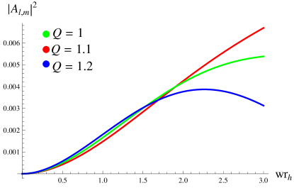
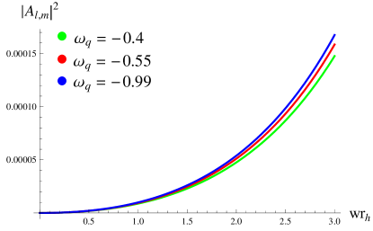
Figure 3: Greybody factor for massless scalar fields corresponding to $\omega_{q}=-0.4$, (left plot) and $Q=0.01$ (right plot) with $l=m=0$, $M=1$ and $a_{0}=0.01=\alpha$.

In order to analyze the significant features of greybody factor, we sketch the expression (55) versus dimensionless parameter $wr_{h}$ and examine its dependence on topological parameters $(Q,a_{0},\alpha,\omega_{q})$ and angular momentum numbers $(l,m)$. It is observed that the absorption probability interpolates smoothly between $0$ and asymptotic value $1$. In Figure 3, we plot the graphs for different choices of charge and state parameters by considering the other variables as fixed quantities. It is found that the greybody factor gets suppressed for larger values of charge (left plot) as expected from the effective potential plot (Figure 1) whereas the higher modes of state parameter depict a slight increase in the absorption probability (right plot).

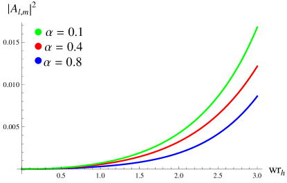
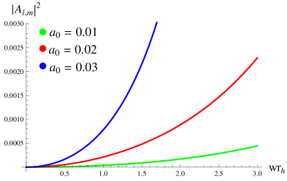
Figure 4: Greybody factor for massless scalar fields corresponding to $a_{0}=0.03$, (left plot) and $\alpha=0.01$ (right plot) with $l=m=0$, $M=1$, $Q=0.1$ and $\omega_{q}=-0.6$.

Figure 4 (left plot) indicates that increase in the strength of quintessence matter $\alpha$ causes a reduction in the emission of scalar fields. Moreover, we obtain that the greybody factor increases comprehensively for the larger modes of rotation parameter (right plot). The impact of positive as well as negative values of $m$ on the greybody factor is displayed in Figure 5. It is noted that an increase in $m$ reduces the emission process while the negative modes of $m$ yield higher values of absorption probability. Finally, the effect of orbital angular momentum on absorption probability is shown in Figure 6. This indicates that low partial wave ($l=1$) leads to smaller values of the greybody factor while higher values of $l$ dominate in the high-energy regions.

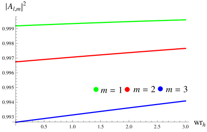
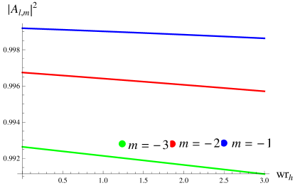
Figure 5: Greybody factor for massless scalar fields corresponding to $l=3$, $\alpha=a_{0}=0.1=Q$, $M=1$ and $\omega_{q}=-0.4$

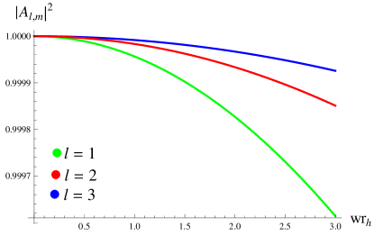
Figure 6: Greybody factor for massless scalar fields corresponding to $m=0$, $\alpha=a_{0}=0.1=Q$, $M=1$ and $\omega_{q}=-0.4$

The total amount of massless particles emitted from a BH per unit time and frequency is given by

$$\frac{d^{2}\tilde{N}}{dtdw}=\frac{1}{2\pi}\sum_{l,m}\frac{1}{e^{\frac{k}{T_{H}}-1}}|\tilde{\emph{A}}_{l,m}|^{2},\quad k=w-\frac{ma_{0}}{r_{h}^{2}+a_{0}^{2}}.$$ (56)

Moreover, the energy emission rate can be expressed as

$$\frac{d^{2}\tilde{E}}{dtdw}=\frac{1}{2\pi}\sum_{l,m}\frac{w}{e^{\frac{k}{T_{H}}-1}}|\tilde{\emph{A}}_{l,m}|^{2},$$ (57)

which, through Eq.(55), has the form

$$\frac{d^{2}\tilde{E}}{dtdw}=\frac{1}{2\pi}\sum_{l,m}\frac{w}{e^{\frac{k}{T_{H}}-1}}\left(1-\left|\frac{\hat{\mathcal{A}}_{2}\hat{\mathcal{H}}_{3}-\hat{\mathcal{A}}_{1}\hat{\mathcal{H}}_{1}}{\hat{\mathcal{A}}_{2}\hat{\mathcal{H}}_{4}-\hat{\mathcal{A}}_{1}\hat{\mathcal{H}}_{2}}\right|^{2}\right).$$ (58)

The dependence of greybody factor on particle as well as spacetime properties changes the various emission rates, accordingly. The absorption cross-section for charged rotating BH surrounded by quintessential field is given as

$$\sigma=\frac{\pi}{w^{2}}\sum_{l,m}|\tilde{\emph{A}}_{l,m}|^{2}.$$ (59)

Using Eq.(55), we have

$$\sigma=\frac{\pi}{w^{2}}\sum_{l,m}\left(1-\left|\frac{\hat{\mathcal{A}}_{2}\hat{\mathcal{H}}_{3}-\hat{\mathcal{A}}_{1}\hat{\mathcal{H}}_{1}}{\hat{\mathcal{A}}_{2}\hat{\mathcal{H}}_{4}-\hat{\mathcal{A}}_{1}\hat{\mathcal{H}}_{2}}\right|^{2}\right).$$ (60)

The absorption cross-section as a function of incident frequency is used to quantify the probability of a certain particle-particle interaction such as scattering, electromagnetic absorption, etc. It exhibits oscillations around the limit of geometrical optics which is a characteristic of diffraction patterns [31].

5 Conclusions

To examine the Hawking radiation spectra emitted from various BH geometries, the greybody factors for different scalar fields have intensively been studied. This paper formulates an analytic expression of the greybody factor for charged rotating BH surrounded by the quintessence, valid in low-energy approximation. Initially, we have investigated the profile of effective potential which originates the absorption probability. The radial equation of motion has been solved analytically at two specific horizons to obtain asymptotic solutions in the form of hypergeometric functions. We have extrapolated these solutions and matched them smoothly to an intermediate regime to obtain a general form of the greybody factor. The energy emission rate and absorption cross-section have been computed for the massless scalar fields.

It is found that the height of effective potential increases with the gradual increase in charge. It is worthwhile to mention here that the electromagnetic force enhances the gravitational pull of the BH which ultimately minimizes the emission rate of Hawking radiation (Figure 1). The larger values of $a_{0}$ decrease the gravitational barrier for the massless scalar fields whereas the higher modes of $l$ have an inverse effect on the effective potential.

The graphical analysis of absorption probability indicates its positive range throughout the considered domain. An increase in $Q$ leads to the reduction of absorption probability (Figure 3) which is also consistent with the literature [32]. It is found that the greybody factor gets suppressed for larger values of $\alpha$ in comparison with [21] whereas the higher modes of rotation parameter show a substantial increase in the emission rate of massless scalar particles. For the orbital angular momentum, partial wave with smaller values reduce the greybody factor as for the rotating BH [33]. It is observed that by taking $\alpha=0$, $Q=0$ and $a_{0}=0$, the line-element reduces to the Kerr-Newman, Kerr and Schwarzschild BH, respectively. Consequently, the analytical expressions of the effective potential and greybody factor reduce to the corresponding BH solutions which are in well-agrement with the literature [6]-[8]. We conclude that the inclusion of charge parameter in the presence of quintessential field significantly affects the potential barrier as well as greybody factor. It would be interesting to study the quasinormal modes resonant phenomena in the background of quintessential BH as done for other BH [34].

Acknowledgement

One of us (QM) would like to thank the Higher Education Commission, Islamabad, Pakistan for its financial support through the Indigenous Ph.D. Fellowship, Phase-II, Batch-III.

References

• [1] Hawking, S.W.: Commun. Math. Phys. 43(1975)199.
• [2] Ford, L.H.: Phys. Rev. D 12(1975)2963; Gubserv, S.S. and Klebanov, I.R.: Phys. Rev. Lett. 77(1996)4491.
• [3] Maldacena, J.M. and Strominger, A.: Phys. Rev. D 55(1997)861.
• [4] Klebanov, I.R. and Mathur, S.D.: Nucl. Phys. B 500(1997)115.
• [5] Kim, W.T. and Oh, J.J.: Phys. Lett. B 461(1999)189.
• [6] Konoplya, R.A.: Phys. Rev. D 66(2002)044009.
• [7] Konoplya, R.A. and Zhidenko, A.: J. High Energy Phys. 06(2004)037.
• [8] Konoplya, R.A. and Zhidenko, A.: Rev. Mod. Phys. 83(2011)793.
• [9] Ngampitipan, T. and Boonserm, P.: J. Phys. Conf. Ser. 435(2013)012027.
• [10] Boonserm, P., Ngampitipan, T. and Visser, M.: J. High Energy Phys. 03(2014)113.
• [11] Toshmatov, B. et al.: Phys. Rev. D 91(2015)083008.
• [12] Ahmad, J. and Saifullah, K.: Eur. Phys. J. C 77(2017)885.
• [13] Ahmad, J. and Saifullah, K.: Eur. Phys. J. C 78(2018)316.
• [14] Dey, S. and Chakrabarti, S.: Eur. Phys. J. C 79(2019)504.
• [15] Stuchlik, Z.: Mod. Phys. Lett. A 20(2005)561.
• [16] Kiselev, V.V.: Class. Quantum Grav. 20(2003)1187.
• [17] Chen, S. and Jing, J.: Class. Quantum Grav. 22(2005)4651; Zhang, Y. and Gui, Y.X.: Class. Quantum Grav. 23(2006)6141; Zhang, Y. et al.: Gen. Relativ. Gravit. 39(2007)1003.
• [18] Chen, S., Wang, B. and Su, R.: Phys. Rev. D 77(2008)124011.
• [19] Hao, L., Ju-Hua, C. and Yong-Jiu, W.: Chin. Phys. B 21(2012)080402.
• [20] Saleh, M. et al.: Astrophys. Space Sci. 33(2011)449.
• [21] Chakrabarty, H., Abdujabbarov, A. and Bambi, C.: Eur. Phy. J. C 79(2019)179.
• [22] Newman, E.T. and Janis, A.I.: J. Math. Phys. 6(1965)915.
• [23] Newman, E. and Penrose, R.: Phys. Rev. Lett. 11(1962)566.
• [24] Newman, E.T., Couch, E. and Chinnapared, K.: J. Math. Phys. 6(1965)918.
• [25] Toshmatov, B. et al.: Phys. Rev. D 89(2014)104017.
• [26] Ghosh, S.G. and Maharaj, S.D.: Eur. Phy. J. C 75(2015)7.
• [27] Toshmatov, B., Stuchlik, Z. and Ahmedov, B.: Eur. Phys. J. Plus 132(2017)98.
• [28] XU, Z. and Wang, J.: Phys. Rev. D 95(2017)064015.
• [29] Flammer, C.: Spheroidal Wave Functions (Stanford University Press, 1957); Goldberg, J.N. et al.: J. Math. Phys. 8(1967)2155.
• [30] Berti, E., Cardoso, V. and Casals, M.: Phys. Rev. D 73(2006)024013; ibid. 109902.
• [31] Sanchez, N.: Phys. Rev. D 18(1978)1030.
• [32] Fernando, S.: Int. J. Mod. Phys. D 26(2017)1750071.
• [33] Creek, S. et al.: Phys. Lett. B 656(2007)102.
• [34] Toshmatov, B. and Stuchlik, Z.: Eur. Phys. J. Plus 132(2017)324.