Quantum $\varphi$-synchronization in coupled optomechanical system with periodic modulation

Abstract

Based on the concepts of quantum synchronization and quantum phase synchronization proposed by A. Mari et al. in Phys. Rev. Lett. 111, 103605 (2013), we introduce and characterize the measure of a more generalized quantum synchronization called quantum $\varphi$-synchronization under which the pairs of variables have the same amplitude and possess the same $\varphi$ phase shift. Naturally, quantum synchronization and quantum anti-synchronization become special cases of quantum $\varphi$-synchronization. Their relations and differences are also discussed. To illustrate these theories, we investigate the quantum $\varphi$-synchronization and quantum phase synchronization phenomena of two coupled optomechanical systems with periodic modulation and show that quantum $\varphi$-synchronization is more general as a measure of synchronization. We also show the phenomenon of quantum anti-synchronization when $\varphi=\pi$.

I Introduction

As a collective dynamic behavior in complex systems, synchronization was first proposed by Huygens in the 17th century Fujisaka and Yamada (1983); Barahona and Pecora (2002). He noticed that the oscillations of two pendulum clocks with a common support tend to synchronize with each other Huygens (1897). Since then, synchronization has been widely studied and applied in classical physics. Furthermore, with the development of quantum mechanics, the concept of quantum synchronization was proposed and widely applied in the fields, such as cavity quantum electrodynamics Zhirov and Shepelyansky (2009); Ameri et al. (2015), atomic ensembles Xu et al. (2014); Xu and Holland (2015); Hush et al. (2015), van der Pol (VdP) oscillators Ameri et al. (2015); Lee et al. (2014); Walter et al. (2014); Es’haqi-Sani et al. (2019), Bose-Einstein condensation Samoylova et al. (2015), superconducting circuit systems Gül (2016); Quijandría et al. (2013), and so on.

In recent years, there has been a growing interest in exploiting synchronization Zalalutdinov et al. (2003) for significant applications in micro-scale and nano-scale systems Galindo and Martín-Delgado (2002). For example, synchronization of two anharmonic nanomechanical oscillators is implemented in Matheny et al. (2014). And, experimentally, the synchronization measure of the system has been realized through optomechanical devices, including the synchronization of two nanomechanical beam oscillators coupled by a mechanical element Shim et al. (2007), two dissimilar silicon nitride micromechanical oscillators coupled by an optical cavity radiation field Zhang et al. (2012), and two nanomechanical oscillators via a photonic resonator Bagheri et al. (2013). These ingenious experiments fully test the theoretical prediction of the synchronization of optomechanical systems. In addition, the relationship between quantum synchronization and the collective behavior of classical systems is also widely concerned, such as quantum synchronization of van der Pol oscillators with trapped ions Lee and Sadeghpour (2013), and quantum-classical transition of correlations of two coupled cavities Lee and Cross (2013). Besides, the role of the environment and the correlation between the subsystems in the system with quantum synchronization, such as entanglement and mutual information, have been discussed as the main influencing factors Giorgi et al. (2012); Liao et al. (2019); Karpat et al. (2019).

Another aspect of synchronization drawing much more attention recently is the generalization of its classical concepts into the continuous-variable quantum systems, such as complete synchronization Pecora and Carroll (1990), phase synchronization Parlitz et al. (1996); Ho et al. (2002), lag synchronization Taherion1 and Lai (1999), and generalized synchronization Zheng and Hu (2000). After Mari et al. introduced the concepts of quantum complete synchronization and quantum phase synchronization Mari et al. (2013), some interesting efforts have been devoted to enhance the quantum synchronization and quantum phase synchronization by manipulating the modulation Shlomi et al. (2015); Amitai et al. (2017), changing the ways of coupling between two subsystems Mari et al. (2013); Mari and Eisert (2012, 2009); Du et al. (2017), or introducing nonlinearity Qiao et al. (2018); Li et al. (2017). Furthermore, the concepts of quantum generalized synchronization, time-delay synchronization as well as in-phase and anti-phase synchronization have also been mentioned in Li et al. (2016); Ying et al. (2014). However, other than the quantum complete synchronization under which the pairs of variables have the same amplitude and phase, the concept of quantum anti-synchronization corresponding to classical anti-synchronization has not been proposed yet. Moreover, a more generalized quantum synchronization can be defined as “the pairs of variables have the same amplitude and possess the same $\varphi$ phase shift” (hereafter referred to as quantum $\varphi$-synchronization), i.e., for $\varphi=\pi$, the pairs of variables, such as positions and momenta, will always have a $\pi$ phase difference with each other Ying et al. (2014). This type of quantum $\varphi$-synchronization is called quantum anti-synchronization. Hence, one will naturally ask how to define and measure the quantum $\varphi$-synchronization?

To shed light on this question, in this work we give the definition of quantum $\varphi$-synchronization for the continuous-variable quantum systems by combining the concept of quantum synchronization and the phenomenon of transition from in-phase to anti-phase synchronization Ying et al. (2014). The paper is organized as follows. In Sec. II, we first reexamine the definitions of quantum complete synchronization and phase synchronization. Based on these concepts, the definition of quantum $\varphi$-synchronization is given, by which the quantum synchronization and quantum anti-synchronization can be treated as special cases of quantum $\varphi$-synchronization. The $\varphi$-synchronization of a coupled optomechanical system with periodic modulation is studied to illustrate our theory in Sec. III. In Sec. IV, a brief discussion and summary are given.

II Measure of quantum synchronization and quantum $\varphi$-synchronization

Unlike the synchronization in classical system, the complete synchronization in quantum system can not be defined straightforwardly, since the fluctuations of the variables in the two subsystems must be strict to the limits brought by the Heisenberg principle. To address this issue, Mari et al. proposed the measure criterion of quantum complete synchronization for continuous variable (CV) systems Mari et al. (2013)

$$S_{c} =\frac{1}{\langle q_{-}(t)^{2}+p_{-}(t)^{2}\rangle},$$ (1)

where $q_{-}(t)=\frac{1}{\sqrt{2}}[q_{1}(t)-q_{2}(t)]$ and $p_{-}(t)=\frac{1}{\sqrt{2}}[p_{1}(t)-p_{2}(t)]$ are error operators. In order to study purely quantum mechanical effects, the changes of variables are generally taken as

$$q_{-}(t)\rightarrow\delta q_{-}(t) =q_{-}(t)-\langle q_{-}(t)\rangle,$$ (2)

$$p_{-}(t)\rightarrow\delta p_{-}(t) =p_{-}(t)-\langle p_{-}(t)\rangle.$$

Then the contribution of the classical systematic error brought by the mean values $\langle q_{-}(t)\rangle$ and $\langle p_{-}(t)\rangle$ in $S_{c}$ can be dropped, and $S_{c}$ will be replaced by the pure quantum synchronization measure

$$S_{q}=\frac{1}{\langle\delta q_{-}(t)^{2}+\delta p_{-}(t)^{2}\rangle}.$$ (3)

This definition requires that the mean values of $q_{-}(t)$ and $p_{-}(t)$ are exactly zero, i.e., $\langle q_{-}(t)\rangle=0$ and $\langle p_{-}(t)\rangle=0$.

Mari et al. have explained that if the averaged phase-space trajectories (limit cycles) of the two systems are constant but slightly different from each other, a classical systematic error can be easily excluded from the measure of synchronization Mari et al. (2013). The mean-value synchronization is also regarded as a necessary condition of pure quantum synchronization Li et al. (2017). It is more reasonable and rigorous to study pure quantum synchronization based on mean-value synchronization. Therefore, we can generalize the definition of quantum complete synchronization into the quantum $\varphi$-synchronization

$$S_{\varphi} =\frac{1}{\langle q^{\varphi}_{-}(t)^{2}+p^{\varphi}_{-}(t)^{2}\rangle},$$ (4)

which does not require mean-value synchronization. The $\varphi$-error operators are defined as $q^{\varphi}_{-}(t)=\frac{1}{\sqrt{2}}[q^{\varphi}_{1}(t)-q^{\varphi}_{2}(t)]$ and $p^{\varphi}_{-}(t)=\frac{1}{\sqrt{2}}[p^{\varphi}_{1}(t)-p^{\varphi}_{2}(t)]$ with

$$q^{\varphi}_{j}(t) =q_{j}(t)\cos(\varphi_{j})+p_{j}(t)\sin(\varphi_{j}),$$ (5)

$$p^{\varphi}_{j}(t) =p_{j}(t)\cos(\varphi_{j})-q_{j}(t)\sin(\varphi_{j}),$$

where the phase $\varphi_{j}=\arctan[\langle p_{j}(t)\rangle/\langle q_{j}(t)\rangle]$, $\varphi_{j}\in[0,2\pi]$. The upper limit of $S_{\varphi}$ is also given by the Heisenberg principle

$$S_{\varphi} =\frac{1}{\langle q^{\varphi}_{-}(t)^{2}+p^{\varphi}_{-}(t)^{2}\rangle}$$ (6)

$$\leq\frac{1}{2\sqrt{\langle q_{-}^{\varphi}(t)^{2}\rangle\langle p_{-}^{\varphi}(t)^{2}\rangle}}$$

$$\leq\frac{1}{2\sqrt{[\langle q_{-}^{\varphi}(t)^{2}\rangle-\langle q^{\varphi}_{-}(t)\rangle^{2}][\langle p_{-}^{\varphi}(t)^{2}\rangle-\langle p^{\varphi}_{-}(t)\rangle^{2}]}}$$

$$\leq\frac{1}{\sqrt{\mid\frac{1}{2}[q^{\varphi}_{1}(t),p^{\varphi}_{1}(t)]+\frac{1}{2}[q^{\varphi}_{2}(t),p^{\varphi}_{2}(t)]\mid^{2}}}$$

$$=1.$$

This means that the closer $S_{\varphi}$ is to 1, the better the quantum $\varphi$-synchronization. Again, let’s take the changes of variables

$$q^{\varphi}_{-}(t)\rightarrow\delta q^{\varphi}_{-}(t)=q^{\varphi}_{-}(t)-\langle q^{\varphi}_{-}(t)\rangle,$$ (7)

$$p^{\varphi}_{-}(t)\rightarrow\delta p^{\varphi}_{-}(t)=p^{\varphi}_{-}(t)-\langle p^{\varphi}_{-}(t)\rangle.$$

The mean values of $q^{\varphi}_{-}(t)$ and $p^{\varphi}_{-}(t)$ are zero when the average amplitude and period of the mean value of the two variables are the same. In this case, $S_{\varphi}$ equals to the pure quantum $\varphi$-synchronization measure $S^{\varphi}_{q}$ mathematically

$$S^{\varphi}_{q} =\frac{1}{\langle\delta q^{\varphi}_{-}(t)^{2}+\delta p^{\varphi}_{-}(t)^{2}\rangle}$$ (8)

$$=\left\langle\frac{1}{2}\left[(\delta p_{1})^{2}+(\delta q_{1})^{2}+(\delta p_{2})^{2}+(\delta q_{2})^{2}\right.\right.$$

$$+2(\delta p_{1}\delta q_{2}-\delta q_{1}\delta p_{2})\sin{\varphi}-2(\delta p_{1}\delta p_{2}+\delta q_{1}\delta q_{2})\cos{\varphi}]\rangle^{-1},$$

where $\varphi=\varphi_{2}-\varphi_{1}$ can be determined by the final steady state. Now let’s explain the relationship between quantum $\varphi$-synchronization and quantum complete synchronization, quantum phase synchronization. We can see from Eq. (8) that the definition of $S^{\varphi}_{q}$ can be reduced into (a) quantum synchronization: if $\varphi=0$, then $S_{q}=S_{q}^{\varphi}$; (b) quantum phase synchronization: if $\langle\delta q^{\varphi}_{-}(t)^{2}\rangle=\langle\delta p^{\varphi}_{-}(t)^{2}\rangle$, then $S_{p}=S_{q}^{\varphi}$. (c) if $\varphi=\pi$, $\widetilde{S}_{q}=S_{q}^{\varphi}$, where $\widetilde{S}_{q}$ can be defined as quantum anti-synchronization. Therefore, quantum synchronization and quantum anti-synchronization are the special cases of quantum $\varphi$-synchronization. But the definition of quantum phase synchronization is slightly different Mari et al. (2013)

$$S_{p}=\frac{1}{2}\langle\delta p^{\varphi}_{-}(t)^{2}\rangle^{-1}=\frac{1}{\langle\delta p^{\varphi}_{-}(t)^{2}+\delta p^{\varphi}_{-}(t)^{2}\rangle}.$$ (9)

Unlike $S_{\varphi}$ in Eq. (6), the measure of quantum phase synchronization $S_{p}$ can exceed $1$. To illustrate these definitions, we next compare quantum $\varphi$-synchronization with quantum synchronization and quantum phase synchronization in coupled optomechanical system with periodic modulation.

III Quantum synchronization, quantum phase synchronization and quantum $\varphi$-synchronization in coupled optomechanical system with periodic modulation

To examine the relations and differences between quantum synchronization, quantum phase synchronization and quantum $\varphi$-synchronization, we consider a coupled optomechanical system with periodic modulation Du et al. (2017); Qiao et al. (2018). Two subsystems are coupled by optical fibers Joshi et al. (2012). Each of them is consisted of a mechanical oscillator coupled with a Fabry-Perot cavity driven by a time-periodic modulated filed (see Fig. 1) Bemani et al. (2017). It’s worth noting that the optomechanical device is experimentally possible. On the one hand, the synchronization of two mechanically isolated nanomechanical resonators via a photonic resonator has been implemented Bagheri et al. (2013). On the other hand, the self-oscillating mechanical resonator in on-fiber optomechanical cavity excited by a tunable laser with periodically modulated power also has been studied Shlomi et al. (2015). Then the Hamiltonian of the whole coupled system can be written as

$$H= \sum_{j=1}^{2}\left\{-\triangle_{j}\left[1+A_{c}\cos(\omega_{c}t)\right]a_{j}^{\dagger}a_{j}+\frac{\omega_{j}}{2}\left(p_{j}^{2}+q_{j}^{2}\right)-ga_{j}^{\dagger}a_{j}q_{j}\right.$$ (10)

$$\left.+iE(a_{j}^{\dagger}-a_{j})\right\}+\lambda\left(a_{1}^{\dagger}a_{2}+a_{2}^{\dagger}a_{1}\right),$$

where $a$ and $a^{\dagger}$ are the creation and annihilation operators, $q_{j}$ and $p_{j}$ are the position and momentum operators of mechanical oscillator with frequency $\omega_{j}$ in $j$th subsystem , respectively Wang et al. (2016); Jin et al. (2017). $\lambda$ is the optical coupling strength and $E$ is the intensity of the driving field. $\Delta_{j}$ is the optical detuning, which is modulated with a common frequency $\omega_{c}$ and amplitude $A_{c}$. $g$ is the optomechanical coupling constant.

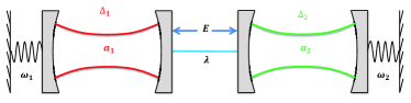
Figure 1: Schematic illustration of coupled optomechanical system with periodic modulation.

To solve time evolution of the dynamical operators $O=q_{j},p_{j},a_{j}$ of the system, we consider the dissipation effects in the Heisenberg picture and utilize the quantum Langevin equation Aspelmeyer et al. (2014). From Eq. (10), the evolution equations of the operators can be written as:

$$\dot{q_{j}}= \omega_{j}p_{j},$$ (11)

$$\dot{p_{j}}= -\omega_{j}q_{j}-\gamma p_{j}+ga_{j}^{\dagger}a_{j}+\xi_{j},$$

$$\dot{a_{j}}= -\left\{\kappa-i\triangle_{j}\left[1+A_{c}\cos(\omega_{c}t)\right]\right\}a_{j}+iga_{j}q_{j}+E$$

$$-i\lambda a_{3-j}+\sqrt{2\kappa}a_{j}^{in},$$

where $\kappa$ is the radiation loss coefficient Jing et al. (2014); Schönleber et al. (2016) and $\gamma$ is mechanical damping rate, respectively. $a_{j}^{in}$ and $\xi_{j}$ are input bath operators and satisfy standard correlation: $\left\langle a^{in\dagger}(t)a^{in}(t^{\prime})+a^{in}(t^{\prime})a^{in\dagger}(t)\right\rangle=\delta(t-t^{\prime})$ and $\frac{1}{2}\langle\xi_{j}(t)\xi_{j^{\prime}}(t^{\prime})+\xi_{j^{\prime}}(t^{\prime})\xi_{j}(t)\rangle=\gamma(2\bar{n}_{bath}+1)\delta_{jj^{\prime}}\delta(t-t^{\prime})$ under the Markovian approximation Wang et al. (2016); Jin et al. (2017), where $\bar{n}_{bath}=1/[\exp\left(\hbar\omega_{j}/k_{B}T\right)-1]$ is the mean occupation number of the mechanical baths which gauges the temperature $T$ of the system Giovannetti and Vitali (2001); Liu et al. (2014); Xu and Li (2015). To solve the set of nonlinear differential operator equations , we need to linearize Eq. (11). There may be several ways to do that, such as using the stochastic Hamiltonian He et al. (2016, 2017), and mean field approximationLi et al. (2015, 2016); Farace and Giovannetti (2012); Mari and Eisert (2012). Here we use the mean field approximation, since it can uncover the effects of mean error and quantum fluctuation on quantum synchronization. Namely, the operators are decomposed into an mean value and a small fluctuation, i.e.

$$O(t)=\langle O(t)\rangle+\delta O(t).$$ (12)

And, as long as $|\langle O(t)\rangle|\gg 1$, the usual linearization approximation to Eq. (11) can be implemented Mari and Eisert (2009). Then, Eq. (11) can be divided into two different sets of equations, one for the mean value

$$\partial_{t}{\langle q_{j}\rangle}= \omega_{j}\langle p_{j}\rangle,$$ (13)

$$\partial_{t}{\langle p_{j}\rangle}= -\omega_{j}\langle q_{j}\rangle-\gamma\langle p_{j}\rangle+g|\langle a_{j}\rangle|^{2},$$

$$\partial_{t}{\langle a_{j}\rangle}= -\left\{\kappa-i\triangle_{j}\left[1+A_{c}\cos(\omega_{c}t)\right]\right\}\langle a_{j}\rangle+ig\langle a_{j}\rangle\langle q_{j}\rangle+E$$

$$-i\lambda\langle a_{3-j}\rangle,$$

and the other for the fluctuation:

$$\partial_{t}{\delta q_{j}}= \omega_{j}\delta p_{j},$$ (14)

$$\partial_{t}{\delta p_{j}}= -\omega_{j}\delta q_{j}-\gamma\delta p_{j}+g(\langle a_{j}\rangle\delta a_{j}^{\dagger}+\langle a_{j}\rangle^{*}\delta a_{j})+\xi_{j},$$

$$\partial_{t}{\delta a_{j}}= -\left\{\kappa-i\triangle_{j}\left[1+A_{c}\cos(\omega_{c}t)\right]\right\}\delta a_{j}+ig(\langle a_{j}\rangle\delta q_{j}$$

$$+\langle q_{j}\rangle\delta a_{j})-i\lambda\delta a_{3-j}+\sqrt{2\kappa}a_{j}^{in}.$$

In Eq. (14), the second-order smaller terms of the fluctuation have been ignored. Then, by defining $u=(\delta q_{1},\delta p_{1},\delta x_{1},\delta y_{1},\delta q_{2},\delta p_{2},\delta x_{2},\delta y_{2})^{\top}$ with $\delta x_{j}=\frac{1}{\sqrt{2}}\left(\delta a_{j}^{\dagger}+\delta a_{j}\right)$ and $\delta y_{j}=\frac{i}{\sqrt{2}}\left(\delta a_{j}^{\dagger}-\delta a_{j}\right)$, Eq. (14) can be simplified to:

$$\partial_{t}{u}=Mu+n,$$ (15)

where $n=(0,\xi_{1},\sqrt{2\kappa}x_{1}^{in},\sqrt{2\kappa}y_{1}^{in},0,\xi_{2},\sqrt{2\kappa}x_{2}^{in},\sqrt{2\kappa}y_{2}^{in})^{\top}$ is the noise vector with $x_{1}^{in}=\frac{1}{\sqrt{2}}\left(a^{in^{\dagger}}+a^{in}\right)$ and $y_{1}^{in}=\frac{i}{\sqrt{2}}\left(a^{in^{\dagger}}-a^{in}\right)$. $M$ is a time-dependent coefficient matrix:

$$M=\left(\begin{array}[]{cc}M_{1}&M_{0}\\ M_{0}&M_{2}\\ \end{array}\right),$$ (16)

with

$$M_{j}=\left(\begin{array}[]{cccc}0&\omega_{j}&0&0\\ -\omega_{j}&-\gamma&\sqrt{2}g\mathrm{Re}(\langle a_{j}\rangle)&\sqrt{2}g\mathrm{Im}(\langle a_{j}\rangle)\\ -\sqrt{2}g\mathrm{Im}(\langle a_{j}\rangle)&0&-\kappa&-F_{j}\\ \sqrt{2}g\mathrm{Re}(\langle a_{j}\rangle)&0&F_{j}&-\kappa\end{array}\right),$$

and

$$M_{0}=\left(\begin{array}[]{cccc}0&0&0&0\\ 0&0&0&0\\ 0&0&0&\lambda\\ 0&0&-\lambda&0\end{array}\right),$$

where $F_{j}=\Delta_{j}[1+A_{c}\cos(\omega_{c}t)]+g\langle q_{j}\rangle$ and the evolution process of matrix element $M(t)$ at any time can be obtained by solving Eq. (13) numerically when the initial conditions are $0$. In order to study the contribution of quantum fluctuation to quantum synchronization, we consider the following covariance matrix:

$$V_{ij}\equiv\frac{1}{2}\langle u_{i}u_{j}+u_{j}u_{i}\rangle.$$ (17)

The evolution of $V$ over time is governed by Li et al. (2015); Mari and Eisert (2009); Wang et al. (2014); Larson and Horsdal (2011):

$$\partial_{t}{V}=MV+VM^{T}+N.$$ (18)

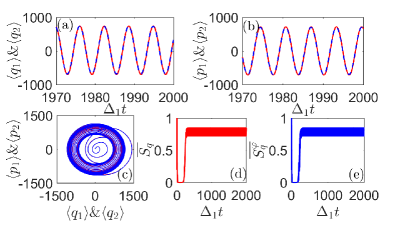
Figure 2: Time evolution of (a) the mean values $\langle q_{1}\rangle$ (red solid line) and $\langle q_{2}\rangle$ (blue dashed line) , (b) the mean values $\langle p_{1}\rangle$ (red solid line) and $\langle p_{2}\rangle$ (blue dashed line), (c) the limit-cycle trajectories in the $\langle q_{1}\rangle\leftrightharpoons\langle p_{1}\rangle$ (red) and $\langle q_{2}\rangle\leftrightharpoons\langle p_{2}\rangle$ (blue) spaces, (d) the measure of quantum synchronization $\overline{S_{q}}$, and (e) the measure of quantum $\varphi$-synchronization $\overline{S^{\varphi}_{q}}$. Parameters are chosen to refer to Mari et al. (2013); Joshi et al. (2012); Li et al. (2017); Du et al. (2017): $\lambda=0.03\Delta_{1}$, $A_{c}=2,\omega_{c}=3\Delta_{1}$. Other parameters are normalized by $\Delta_{1}=1$,$\Delta_{2}=1.005\Delta_{1}$,$\omega_{1}=\Delta_{1}$,$\omega_{2}=\Delta_{2}$, $g=0.005\Delta_{1}$, $\gamma=0.005\Delta_{1}$, $\kappa=0.15\Delta_{1}$, $E=100\Delta_{1}$.

The noise matrix $N=\mathrm{diag}(0,\gamma(2\bar{n}_{bath}+1),\kappa,\kappa,0,\gamma(2\bar{n}_{bath}+1),\kappa,\kappa)$ satisfying $N_{ij}\delta(t-t^{{}^{\prime}})=\frac{1}{2}\langle\xi_{i}(t)\xi_{j}(t^{{}^{\prime}})+\xi_{j}(t^{{}^{\prime}})\xi_{i}(t)\rangle$. Hence, Eq. (3), Eq. (8) and Eq. (9) can be rewritten in terms of $V_{ij}$

$$S_{q}= \left[\frac{1}{2}\left(V_{11}+V_{22}+V_{55}+V_{66}-V_{15}-V_{51}-V_{62}-V_{26}\right)\right]^{-1},$$ (19)

$$S^{\varphi}_{q}= \left[\frac{1}{2}(V_{11}+V_{22}+V_{55}+V_{66}+2V_{25}\sin{\varphi}-2V_{16}\sin{\varphi}\right.$$

$$-2V_{26}\cos{\varphi}-2V_{15}\cos{\varphi})]^{-1},$$

$$S_{p}= [V_{11}(\sin{\varphi_{1}})^{2}+V_{22}(\cos{\varphi_{1}})^{2}+V_{55}(\sin{\varphi_{2}})^{2}$$

$$+V_{66}(\cos{\varphi_{2}})^{2}-2V_{12}\sin{\varphi_{1}}\cos{\varphi_{1}}-2V_{15}\sin{\varphi_{1}}\sin{\varphi_{2}}$$

$$+2V_{16}\sin{\varphi_{1}}\cos{\varphi_{2}}+2V_{25}\cos{\varphi_{1}}\sin{\varphi_{2}}$$

$$-2V_{26}\cos{\varphi_{1}}\cos{\varphi_{2}}-2V_{56}\cos{\varphi_{2}}\sin{\varphi_{2}}]^{-1},$$

and their evolutions can be derived by solving Eq. (13), Eq. (15) and Eq. (18). In addition, under different parameters, the calculated time-averaged synchronization

$$\overline{S_{o}}(t)=\lim_{T\rightarrow\infty}\frac{1}{T}\int_{0}^{T}S_{o}(t)dt$$ (20)

is used as the synchronization measure in the asymptotic steady state of the system, where $o=\varphi,p$. According to $R-H$ criterion DeJesus and Kaufman (1987), all the eigenvalues of coefficient matrix $M$ will be negative after a temporary evolutionary process. Hence, a stable limit cycle solution representing a periodic oscillation will exit Geng et al. (2018).

As we discussed in the last section, if $\varphi=0$, which requires the condition of mean-value complete synchronization, i.e., $\langle q_{-}(t)\rangle=\langle q_{1}(t)\rangle-\langle q_{2}(t)\rangle=0$ , $\langle p_{-}(t)\rangle=\langle p_{1}(t)\rangle-\langle p_{2}(t)\rangle=0$, the measures of quantum $\varphi$-synchronization and quantum synchronization are equivalent, i.e., $S^{\varphi}_{q}=S_{q}$. As shown in Fig. 2(a), $\langle q_{1}(t)\rangle$ and $\langle q_{2}(t)\rangle$ are found to oscillate exactly in phase when entering the stable state. The same conclusion holds for $\langle p_{1}(t)\rangle$ and $\langle p_{2}(t)\rangle$ in Fig. 2(b). In Fig. 2(c), the evolutions of $\langle q_{1}(t)\rangle\leftrightharpoons\langle p_{1}(t)\rangle$ and $\langle q_{2}(t)\rangle\leftrightharpoons\langle p_{2}(t)\rangle$ of the two oscillators trend to an asymptotic periodic orbit (i.e. the two limit cycles tend to be consistent), which indicates that the system is stable. And, Fig 2(d) and (e) show that the changes in $\overline{S_{q}}$ and $\overline{S^{\varphi}_{q}}$ over time are exactly the same. When the mean-value synchronization is not complete, as shown in Fig. 3(a) and 3(b), there exists a phase advance between $\varphi_{2}$ and $\varphi_{1}$, i.e $\varphi=\varphi_{2}-\varphi_{1}=\arctan[\langle p_{2}(t)\rangle/\langle q_{2}(t)\rangle]-\arctan[\langle p_{1}(t)\rangle/\langle q_{1}(t)\rangle]\approx 0.2\pi$. Similarly, the two consistent limit cycles are shown in Fig. 3(c), indicating that the evolution of the system can still reach a steady state when mean-value is not complete synchronization.

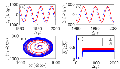
Figure 3: Time evolution of (a) the mean values $\langle q_{1}\rangle$ (red solid line) and $\langle q_{2}\rangle$ (blue dashed line), (b) the mean value $\langle p_{1}\rangle$ (red solid line) and $\langle p_{2}\rangle$(blue dashed line), (c) the limit-cycle trajectories in the $\langle q_{1}\rangle\leftrightharpoons\langle p_{1}\rangle$ (red) and $\langle q_{2}\rangle\leftrightharpoons\langle p_{2}\rangle$ (blue) spaces, and (d) time evolution of the measure of quantum synchronization $\overline{S_{q}}$ [the red (upper) line] and quantum $\varphi$-synchronization $\overline{S^{\varphi}_{q}}$ [the blue (lower) line] with $\lambda=0.14\Delta_{1}$ and $A_{c}=1,\omega_{c}=2\Delta_{1}$. The other parameters are the same as in Fig. 2.

.

However, quantum synchronization $\overline{S_{q}}$ and quantum $\varphi$-synchronization are different as shown in Fig. 3(d). This is because the definition of quantum $\varphi$-synchronization takes the effect of mean-value incomplete synchronization into account. The quantum $\varphi$-synchronization is then more general and rigorous than quantum synchronization. As the mean-value incomplete synchronization will break the condition for Eq. (2), the contribution of $\langle q_{-}(t)\rangle$ and $\langle p_{-}(t)\rangle$ to the quantum complete synchronization $S_{c}$ is much greater than that of the quantum fluctuation. Besides, the mean-value incomplete synchronization will always occur with the change of parameters. As shown in Fig. 4, different phase differences $\varphi$ will be generated by the different modulation frequency $\omega_{c}$. And similar phenomena have been shown in Ying et al. (2014). Therefore, it is necessary to give the quantum synchronization when mean-value synchronization is not complete, namely quantum $\varphi$-synchronization.

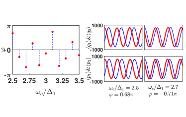
Figure 4: Discrete point diagram (left) of the phase $\varphi$ versus modulation frequency $\omega_{c}$ when the system reaches steady state. The time evolution (right) of the mean values $\langle q_{1}\rangle\&\langle p_{1}\rangle$ (red thick line) and $\langle q_{2}\rangle\&\langle p_{2}\rangle$ (blue thin line) with two values of $\omega_{c}$ from the left panel. The parameter $\lambda=0.14\Delta_{1}$, $A_{c}=1$ and other parameters are the same as in Fig. 2.

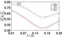
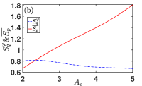
Figure 5: Mean values of the quantum phase synchronization measure $\overline{S_{p}}$ (red solid line) and quantum $\varphi$-synchronization measure $\overline{S^{\varphi}_{q}}$ (the blue dotted line) as a function of (a) the optical coupling coefficient $\lambda$ with $A_{c}=2$, $\omega_{c}=3\Delta_{1}$, (b) the modulation frequency $A_{c}$ with $\lambda=0.03\Delta_{1}$, $\omega_{c}=3\Delta_{1}$. The other parameters are the same as in Fig. 2.

Moreover, the quantum $\varphi$-synchronization also can be related to the quantum phase synchronization. As shown in Fig. 5(a), both quantum $\varphi$-synchronization $\overline{S_{q}^{\varphi}}$ and quantum phase synchronization $\overline{S_{p}}$ first decrease and then increases as the optical coupling strength $\lambda$ increases, and the changing trend of $\overline{S_{p}}$ and $\overline{S^{\varphi}_{q}}$ with $\lambda$ is accordant. When $\lambda=0.016\Delta_{1}$, both $\overline{S_{\varphi}}=0.58$ and $\overline{S_{p}}=0.36$ are minimized. This means that $\langle\delta q_{-}^{\varphi}(t)^{2}\rangle$ is approximately proportional to $\langle\delta p_{-}^{\varphi}(t)^{2}\rangle$ ($\langle\delta q_{-}^{\varphi}(t)^{2}\rangle>\langle\delta p_{-}^{\varphi}(t)^{2}\rangle$). In this case, the measure of $\varphi$-synchronization is accordance with that of the phase synchronization. When $\langle\delta q_{-}^{\varphi}(t)^{2}\rangle=\langle\delta p_{-}^{\varphi}(t)^{2}\rangle$, the two definitions are the same. However, if $\langle\delta q_{-}^{\varphi}(t)^{2}\rangle$ has no linear relation with $\langle\delta p_{-}^{\varphi}(t)^{2}\rangle$, the definitions of $\varphi$-synchronization and phase synchronization are quite different as shown in Fig. 5(b). In Fig. 5(b), the quantum $\varphi$-synchronization $\overline{S^{\varphi}_{q}}$ becomes worse when the modulation amplitude $A_{c}$ increases. While the quantum phase synchronization $\overline{S_{p}}$ is significantly enhanced. This difference is due to the fact that the quantum $\varphi$-synchronization takes both of $\langle\delta q_{-}^{\varphi}(t)^{2}\rangle$ and $\langle\delta p_{-}^{\varphi}(t)^{2}\rangle$ into consideration, while the quantum phase synchronization only considers $\langle\delta p_{-}^{\varphi}(t)^{2}\rangle$. This also results in quantum phase synchronization $\overline{S_{p}}$ exceeding 1 as shown in Fig. 5(b). However quantum $\varphi$-synchronization is still less than $1$ due to the Heisenberg principle, which has also been demonstrated in Eq. (6).

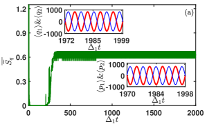
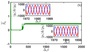
Figure 6: The evolution of the quantum synchronization $\overline{\widetilde{S}_{q}}$ (green solid line), and the mean value $\langle q_{1}\rangle\&\langle p_{1}\rangle$ (red thick line), $\langle q_{2}\rangle\&\langle p_{2}\rangle$ (blue thin line) when the system is stable with (a) $\lambda=0.3\Delta_{1}$ and $A_{c}=1.5,\omega_{c}=2\Delta_{1}$, (b) $\lambda=0.2\Delta_{1}$ and $A_{c}=1,\omega_{c}=2\Delta_{1}$. The other parameters are the same as in Fig. 2.

When $\varphi=\pi$, the $\varphi$-error operators become $q^{\pi}_{-}(t)=\frac{1}{\sqrt{2}}[q_{1}(t)+q_{2}(t)]$ and $p^{\pi}_{-}(t)=\frac{1}{\sqrt{2}}[p_{1}(t)+p_{2}(t)]$. The quantum $\varphi$-synchronization becomes quantum anti-synchronization, i.e.,

$$\widetilde{S}_{q}\equiv S^{\pi}_{q} =\frac{1}{\langle\delta q^{\pi}_{-}(t)^{2}+\delta p^{\pi}_{-}(t)^{2}\rangle}$$ (21)

$$=\left\langle\frac{1}{2}\left[(\delta p_{1}+\delta p_{2})^{2}+(\delta q_{1}+\delta q_{2})^{2}\right]\right\rangle^{-1}.$$

We can also find this phenomenon of quantum anti-synchronization in coupled optomechanical system under certain parameters. As shown in Fig. 6, quantum anti-synchronization is that the mean-value is anti-synchronization and quantum $\varphi$-synchronization is not zero.

IV Conclusions

In summary, we have introduced and characterized a more generalized concept called quantum $\varphi$-synchronization. It can be defined as the pairs of variables which have the same amplitude and possess same $\varphi$ phase shift. The measure of the quantum $\varphi$-synchronization has also been defined with the phase difference $\varphi$. Therefore, the quantum synchronization and quantum anti-synchronization can be treated as the special cases of quantum $\varphi$-synchronization. Besides, the quantum phase synchronization can also be related with the quantum $\varphi$-synchronization. As an example, we have investigated the quantum $\varphi$-synchronization and quantum phase synchronization phenomena of two coupled optomechanical systems with periodic modulation. It has been shown that quantum $\varphi$-synchronization is more general as a measure of synchronization than the quantum synchronization. We have also showed the different affections of the optical coupling coefficient and the modulation amplitude on the quantum phase synchronization and the quantum $\varphi$-synchronization. These two definitions of synchronization are only accordant with each in the case that $\langle\delta q_{-}^{\varphi}(t)^{2}\rangle$ is approximately proportional to $\langle\delta p_{-}^{\varphi}(t)^{2}\rangle$. Based on quantum $\varphi$-synchronization, the quantum anti-synchronization phenomenon has also been defined and observed for $\varphi=\pi$ under some parameters. Therefore, the definition of quantum $\varphi$-synchronization provides a new way to study the quantum synchronization of continuous variable systems. In addition, it is interesting in the future to study the linearization method by using the stochastic Hamiltonian He et al. (2016, 2017) and its influence on the quantum $\varphi$-synchronization.